Effect of the orientational relaxation on the collective motion of patterns formed by self-propelled particles.

Abstract

We investigate the collective behavior of self-propelled particles (SPPs) undergoing competitive processes of pattern formation and rotational relaxation of their self-propulsion velocities. In full accordance with previous work, we observe transitions between different steady states of the SPPs caused by the intricate interplay among the involved effects of pattern formation, orientational order, and coupling between the SPP density and orientation fields. Based on rigorous analytical and numerical calculations, we prove that the rate of the orientational relaxation of the SPP velocity field is the main factor determining the steady states of the SPP system. Further, we determine the boundaries between domains in the parameter plane that delineate qualitatively different resting and moving states. In addition, we analytically calculate the collective velocity $\vec{v}$ of the SPPs and show that it perfectly agrees with our numerical results. We quantitatively demonstrate that $\vec{v}$ does not vanish upon approaching the transition boundary between the moving pattern and homogeneous steady states.

1 Introduction

One of the most intriguing aspects of the collective behavior of a system of self-propelled (active) particles (SPP) [1], is that the motion of each individual particle can cause an organized (”collective”) motion of the SPP system as a whole. At high concentrations of SPPs, the described collective motion is known to occur in systems of active colloids that form regular patterns termed ”active crystals” in [2]. The presence of active drive makes the properties of the described ”active crystals” very different from crystals formed by ordinary ”passive” colloids. In particular, self-propulsion of colloidal particles can significantly lower [3, 4] the concentration threshold of the entropy-driven clustering relative to that observed in the system of passive colloids. Moreover, an additional energy associated with the individual motion of the SPPs can be consumed not only by shifting the crystallization point of the SPP system, but also by inducing the organized motion of the SPPs. In this scenario, the orientational interactions between the individual SPPs can cause an essentially non-equilibrium state, where the SPP system moves in a direction chosen by symmetries of the patterns formed by these SPPs. The described states of collective motion have been observed experimentally in many relevant biological systems, ranging from bacteria colonies [5, 6, 7, 8] to the flocks of birds [9, 10], which explains the high interest in understanding the physical effects underlying these states. Despite essential theoretical progress [1] in the field achieved over the last decade, many aspects of the described collective behavior of SPPs still remain rather obscure. One of such key aspects addressed in the present work, is the relative significance of the tendency of SPPs to form patterns and of the orientational relaxation of their velocities for the formation of moving and resting steady states of the SPP system.

By making use of the minimal model described below, we demonstrate that the orientational relaxation of the SPP velocities is the main factor playing in favor of suppressing the collective motion of the SPPs caused by their self-propulsion. More specifically, we will show that the transition between the observed moving ordered state, resting ordered state and disordered (homogeneous) state can be induced solely by changing the rate of the orientational relaxation of the SPPs. According to our exact results described below, the individual motion of SPPs always causes a tendency towards collective motion of the whole SPP system. In this sense, there exists no single threshold magnitude of the active drive that delineates the regimes of moving and resting states. The main factor that suppresses the collective motion of the SPPs is a sufficiently quick orientational relaxation of the local orientation of the SPP velocities quantified by the ”polarization” field $\mathbf{P}(\vec{r})$.

2 The model

In order to rationalize the described interplay between the tendencies of the active SPP system to the crystallization and collective motion, it is instructive to study a modification of the well-established colloid crystallization model that would adequately account for the active drive of the colloids. A minimal model of that type has been recently developed in [2], by combining the Phase-Field-Crystal (PFC) model [11, 12, 13] and Toner-Tu (TT) [10] approach describing the kinetic flocculation with the effect of the orientational order of flocks taken into account. Owing to its transparency and simplicity, this model provides an excellent framework for studying the complicated interplay between the spatial and orientational ordering of the SPPs. Although this pioneering work provides very useful insight into the nature of the collective behavior of SSPs, it does not give a systematic account for possible transitions between moving and resting states of SPPs depending on the relative significance of the involved effects. In the present work, we use a slightly modified version of the described model with the objective to construct the exact ”phase diagram” describing all the possible collective states of the SPPs, as well as the transition boundaries between them. In addition, we investigate, both analytically and numerically, the dependence of the velocity of the collective motion on the involved parameters. As we demonstrate below, this detailed investigation leads to a new understanding of the relative role of the involved effects (e.g. pattern formation and rotational diffusion) in the formation of the observed moving and resting patterns in the SPP system.

Having implemented the above outlined strategy of combining the PFC and TT approaches, we employ the above outlined idea of describing the correlations between the density $\rho(\vec{r})$ and orientational $\vec{P}({\vec{r}})$ fields with help of coupled PFC and TT equations. Note that the main quantity of interest $\rho$ termed ”density” in the above for the sake of convenience, is assumed to have no limitations with respect to the domain of values it can assume. Similarly as in the standard PFC approach, this quantity should be understood as an order parameter (e.g. a density excess over the critical density). Therefore, $\rho$ can assume, in particular, negative values. Note that additional limitations on the domain of possible values of $\rho$ imposed by specific physical conditions can be easily incorporated into the described model without causing a loss of its generality. One such possibility arises from properly defining the average density $\bar{\rho}$, considered an input parameter of the model.

For the sake of tractability, we use a simplest possible form of the dynamical equation for the vector quantity $\vec{P}$, termed ”polarization” hereafter, describing the orientational order in the field of the SPP velocities. This equation of the form

$$\frac{\partial\vec{P}}{\partial t}=-\tau^{-1}\left(1-\gamma\nabla^{2}\right)\vec{P}-v_{0}\vec{\nabla}\rho$$ (1)

has been first empirically obtained in [14], by making a comparison with the results of the simulations for SPP disks. Note that the terms on the right hand side (r.h.s.) of Eq.(1) containing $\vec{P}$ can be obtained by dropping the non-linear terms in the original TT equations. The generalization of Eq.(1) containing additional non-linear terms has been independently obtained in [2]. Coupling of the orientational order to the density field is described by the last pressure-like gradient term in the r.h.s. of Eq.(1) featuring the constant magnitude $v_{0}$ of the self-propulsion velocity of the SPPs. The coefficients $\tau^{-1}$ and $\gamma$ quantify, respectively, the relaxation rate due to the orientational diffusion and significance of the spatial dispersion of the polarization.

Note that the simple diffusion equation for density $\rho$ used in [14] is not suited for describing the formation of periodic patterns of the SPP density needed to mimic the crystallization of SPPs in our approach. In order to improve this feature of the model, critical for its applicability to the case of active crystals under consideration, we follow [2] and employ the PFC equation for the density $\rho(\vec{r})$ of the form

$$\frac{\partial\rho}{\partial t}=\nabla^{2}\left[\omega(\nabla)\rho+(\bar{\rho}+\rho)^{3}\right]-v_{0}\vec{\nabla}\cdot\vec{P},$$ (2)

where we have separated out the average density $\bar{\rho}$ for the sake of convenience. Here,

$$\omega(\nabla)=-\epsilon+\left(q^{2}+\nabla^{2}\right)^{2}$$ (3)

is the $4$th-order differential operator with the only control parameter $\epsilon$ (reduced deviation from the critical temperature), inherited from the standard PFC model [11, 13, 15]. Recall that in this model the positive (negative) values of $\epsilon$ correspond to the ordered patterned (homogeneous) steady states of the density field. The morphology of patterns formed at positive $\epsilon$ is determined by the average density $\bar{\rho}$. Note that the only difference that distinguishes the standard PFC equation from its modification in Eq.(2) is the last term in its r.h.s. describing the coupling of the density structure to the polarization field.

It is important to note an essential difference between the structures of the equations in Eq.(2) and Eq.(1). Eq.(2) is a non-linear equation for the density coupled to Eq.(1) through the linear coupling term $v_{0}\vec{\nabla}\cdot\vec{P}$. Eq.(1) is, in contrast, a linear differential equation, which greatly simplifies the analysis of the coupled dynamics of the fields $\rho$ and $\vec{P}$. Specifically, in the frameworks of the proposed linear model for the dynamics of $\vec{P}$, the effect of the orientational field on the pattern formation and collective motion of SPPs can be fully understood in terms of the relation among the relaxation rate $\tau^{-1}$ and reduced self-propulsion velocity $v_{0}$. In the extreme case of quick relaxation of the orientational field $\vec{P}$ ($q\tau v_{0}\ll 1$), the spatial structure of the polarization field $\vec{P}$ immediately adjusts to the structure of the density field $\rho$ of the SPPs. Physically, this regime corresponds to sufficiently large undercooling, where the local mobility of the SPP domains depends only on their density, so that the most ”crowded” domains have the smallest local velocities. In the symmetric density phases, the individual motion of the SPP domains moving in the opposite directions averages out, thus resulting in the resting state. In this case, the orientational relaxation of $\vec{P}$ causes no qualitative difference in the spatial structure of $\rho$ relative to the predictions of the standard PFC model. As will be shown in what follows, the described quick relaxation of $\vec{P}$ causes only a quantitative correction to the PFC control parameter $\epsilon$ in Eq.(3) that leads to a shift of the phase boundary separating the domains of patterns and homogeneous SPP phase. In the opposite case $q\tau v_{0}\gg 1$ of slow orientational relaxation, a more complicated response of the density field to the orientational relaxation is observed. In particular, slow relaxation of $\vec{P}$ results in the occurrence of steady states in the form of moving patterns. In contrast to the former case of the quick relaxation of $\vec{P}$, this case cannot be reduced to any modification of the PFC model.

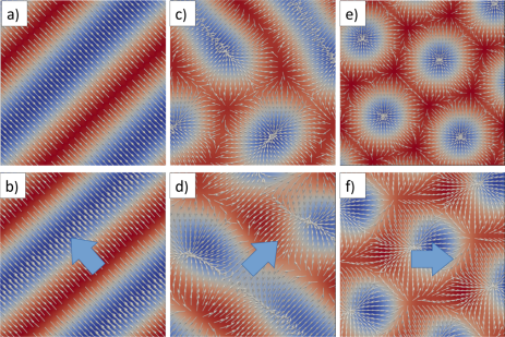
Figure 1: Examples of the morphologies of resting (a, c, e) and moving (b, d, f) patterns obtained from the performed iso-geometric finite element analysis of Eqs.(1-2) for the selected values of the control parameters. In all the examples $\epsilon=1$, $v_{0}=0.3$, $\gamma=0$. Left column: $\bar{\rho}=0$, a) $\tau^{-1}=0.30$, b) $\tau^{-1}=0.20$. Middle column: $\bar{\rho}=0.1$, c) $\tau^{-1}=0.30$, d) $\tau^{-1}=0.20$. Right column: $\bar{\rho}=0.2$, e) $\tau^{-1}=0.30$, f) $\tau^{-1}=0.20$. The blue arrows show the directions of the collective drift of the SPPs. The glyph vectors indicate the direction and magnitude of the polarization field $\vec{P}(\vec{r})$.

3 Linear stability analysis

The above outlined qualitative picture can be rationalized by employing an analytical linear stability analysis of the simultaneous Eqs.(1-2). The obtained analytical prediction for the phase-diagram of pattern formation in the system of SPPs are found to be in perfect agreement with that obtained from the numerical solution of the same equations. We attribute this good agreement to the linear character of Eq.(1) that captures the effects of the orientational field on the density structure on the linear response level.

Linear stability analysis needs to be performed by taking into account the actual morphology of the patterns occurring in the SPP system under investigation. The possible morphologies are determined (see Fig.1) by numerically solving Eqs.(1-2) as described below. These morphologies are found out to be largely the same as those observed in the standard PFC model. For the sake of brevity, we do not discuss different morphologies (e.g. checkerboard and zig-zag lamellae morphologies) that have been observed by us only in the extreme cases of strong coupling $v_{0}\sim 1$ or for large values of $\epsilon\sim 3$. Neither do we analyze non-periodic patterns that occur as ”metastable” states between the lamellae and hexagonal morphologies (see Fig. 1 c, d). It turns out that the morphology of the patterns affects neither the collective velocity nor the shift in the crystallization temperature. This observation gives a rational for restricting our analysis to the cases of lamellae and hexagonal morphologies known from the standard PFC model.

In addition to the well studied resting steady states occurring in the standard PFC, one needs to take into account the possibility that the patterns can move with constant velocity $v$, which complicates the associated mathematical development. The simplest observed one-dimensional morphology, the lamellae morphology (see Fig. 1 a,b)), is comprised of parallel stripes (rolls) that show no spatial variation along their axes. The structure of the lamellae morphology of a given periodicity $\frac{2\pi}{|\vec{k}|}$ can therefore be described by a single wave vector $\vec{k}$ perpendicular to the stripes. For the sake of simplicity, we chose to work in the coordinate frame associated with the wave vector $\vec{k}$ pointing in the direction of the $x$-axis of this frame. With the described choice of the coordinate frame, a set of equations given by Eqs.(1-2) reduces to two coupled equations for $\rho$ and $P_{x}$ with $P_{y}=0$. Periodic modes of the density and orientational fields corresponding to the lamellae morphology moving with velocity $\vec{v}$ can therefore be described by a linear combination of the plane waves $\sim\exp{(\pm ik(x\pm|\vec{v}|t))}$ having different amplitudes and wave numbers $k=|\vec{k}|$. An important feature of the fields $\rho$ and $P_{x}$ that needs to be taken into account in the performed linear analysis, is the phase shift between these periodic fields that can be elucidated by a comparison of the numerical results shown in Figs. 1a) and 1b). We describe this shift by employing the following forms of the fields $\rho\sim\cos{(k(x-vt))}$ and $P_{x}\sim\sin{(k(x+\Delta x-vt))}$. Substituting these expressions into the simultaneous equations Eqs.(1-2), linearizing with respect to the amplitudes of the fields $\rho$ and $P_{x}$, and deriving the consistency conditions for the obtained algebraic linear homogeneous equations for the amplitudes, one arrives at

$$(v^{2}-v_{0}^{2}-v(k\tilde{\tau})^{-1}\tan{(k(\tilde{x}+\Delta x))})\tan{(k\tilde{x})}=$$

$$(\tilde{\epsilon}-(k^{2}-q^{2})^{2})(vk-\tilde{\tau}^{-1}\tan{(k(\tilde{x}+\Delta x))}),$$ (4)

where $\tilde{\epsilon}=\epsilon-3\bar{\rho}^{2}$, $\tilde{\tau}=\tau(1+\gamma k^{2})^{-1}$ and $\tilde{x}=x-vt$. Note that due to the presence of the gradient term in the operator $\omega(\nabla)$ in Eq.(2), the described linearization of Eqs.(1-2) always admits the additional constant solution corresponding to the wave vector $k=0$. Hereafter, we omit this trivial solution that is inherent to the nature of the used ”conserved” PFC equation that preserves the average SPP density.

Eq.(3) admits the solution $\Delta x=0$, $v=0$,

$$\tilde{\epsilon}=v_{0}^{2}\tilde{\tau}+(k^{2}-q^{2})^{2},$$ (5)

which describes the stationary (resting) steady state. It is important to note that this case corresponds to the zero phase shift $\Delta x=0$. This observation quantitatively corroborates the above qualitative consideration that the field of the polarization is in phase with the gradient of the density field in the stationary steady state of the SPP system. In this case, the solution to the linearized equations obtained from Eqs.(1-2) is fully determined by the dispersion relation given by Eq.(5).

In the case of non-zero velocities of the collective motion, Eq.(3) reduces to the explicit expressions for the dispersion relation $\tilde{\epsilon}(k)$, collective velocity $v$ and phase shift $q\Delta x$ of the form

$$\tilde{\epsilon}=k^{-2}\tilde{\tau}^{-1}+(k^{2}-q^{2})^{2},\quad v^{2}=v_{0}^{2}-k^{-2}\tilde{\tau}^{-2},$$ (6)

$$\tan{(k\Delta x)}=kv\tilde{\tau}.$$ (7)

The dispersion relations $\tilde{\epsilon}$ given by Eq. (5) and Eq. (6) determine the non-trivial values of the critical wave numbers that delineate the regions of stability and instability of the solutions of Eqs. (1-2), corresponding to the resting and moving steady states, respectively. According to these relations, the obtained solution of the linearized dynamical equations is unstable in a band of wave numbers in the vicinity of $k=q$. In the presence of non-linear term $\sim(\rho+\bar{\rho})^{3}$ in the r.h.s. of Eq.(2), the exponentially growing modes, causing the instabilities, become suppressed so that they saturate to a finite limit with increasing the time. Similarly as in the standard PFC [12], this suppression results in shrinking the described instability band to a single critical wave number $q$ that corresponds to the only stable mode. Near the onset of the non-linear instability, one can therefore expand the r.h.s. of Eq.(5) and Eq. (6) at $k=q$. Up to the leading order these expansions read,

$$\tilde{\epsilon}_{R}=v_{0}^{2}\tau(1+\gamma q^{2})^{-1},\quad\tilde{\epsilon}_{L}=q^{-2}\tau^{-1}(1+\gamma q^{2})$$ (8)

$$v^{2}=v_{0}^{2}-q^{-2}\tau^{-2}(1+q^{2}\gamma)^{2},$$ (9)

respectively.

Note that the above calculation is valid only for the simplest case of the one-dimensional roll patterns. In order to obtain the dispersion relation and collective velocity for more complicated two-dimensional pattern morphologies, one needs to use a linear combination of the considered roll solutions, corresponding to symmetries of these morphologies. For the case of the hexagonal patterns shown in Fig. 1 e),f), an appropriate linear combination of the roll solutions, admitted by the linearization of Eqs.(1-2), reads

$$\sum\limits_{l=1}^{3}r_{l}\cos{(k\vec{k}_{l}\cdot\vec{\tilde{r}})},\quad\sum\limits_{l=1}^{3}p_{l}^{x,y}\sin{(k\vec{k}_{l}\cdot(\vec{\tilde{r}}+\Delta\vec{r}_{l}))},$$ (10)

where $r_{l}$, $p_{l}^{j}$ are, respectively, the amplitudes of the density field and the $j$th component of the polarization field, $\vec{\tilde{r}}=\vec{r}-\vec{v}_{l}t$, and $k\Delta\vec{r}_{l}$ are the phase shifts of the polarization field. The vectors $\vec{k}_{l}$, associated with different roll modes that form hexagons upon interference, are given by $\vec{k}_{1}=\vec{e}_{x}$, $\vec{k}_{2}=(-\vec{e}_{x}+\sqrt{3}\vec{e}_{y})/2$, and $\vec{k}_{3}=(-\vec{e}_{x}-\sqrt{3}\vec{e}_{y})/2$, $\vec{e}_{x}$ and $\vec{e}_{y}$ being the position vectors associated with a chosen Cartesian coordinate frame. Note that $|\vec{k}_{1}|=|\vec{k}_{2}|=|\vec{k}_{3}|=1$. Applying the procedure used above for the case of a single roll solution to each of the exponential terms given in the r.h.s. of Eq.(10), one arrives at a set of three consistency conditions that lead to an explicit expression for the dispersion relation, velocities $\vec{v}_{l}$ and phase shifts $\Delta\vec{r}_{l}$. The thus obtained dispersion relations $\tilde{\epsilon}(k)$ prove to be the same as those given by Eq.(8) for the one-roll solution in the cases of zero ($\epsilon_{R}$) and non-zero ($\epsilon_{L}$) collective velocities, respectively. The velocities of the rolls are obtained from the above consistency conditions in the form $\vec{v}_{l}=v\vec{k}_{l}$, with $v$ given by Eq.(9). Eq.(10) therefore describes the three rolls, independently moving with the same velocity in the directions normal to their axes. Note that for the considered hexagonal morphology, the quantity $v$ describes the reduced temporal frequency $qv$ of changing the hexagonal patterns in time, and has been called ”velocity” only for the sake of unifying the description with the one-dimensional case. The phase shifts are obtained in the form $\Delta\vec{r}_{l}=\Delta x\vec{k}_{l}$ with $\Delta x$ given by Eq. (7).

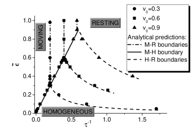
Figure 2: Quasi-phase diagram of moving and resting SPP steady states for the selected values of the coupling $v_{0}$ in terms of the rate $\tau^{-1}$ of the orientational relaxation and the reduced control parameter $\tilde{\epsilon}$ for $\gamma=0.5$, $q=1$: comparison of the analytical predictions by Eqs.(6-8) (solid line) and numerical results (scatter points).

Two important observations regarding the obtained analytical results given by Eqs.(6,8,9) are in order here. First, the r.h.s. of the expressions for the critical control parameter given by Eq.(8) does not depend on the average density $\bar{\rho}$. Recall that parameter $\bar{\rho}$ in the PFC equation for the SPP density given by Eq.(2), is responsible for controlling the morphology of the patterns. Therefore, the above observation speaks in favor of the statement, alluded in the introductory part, that the shape of the boundaries delineating the steady states of the SPP system does not depend on the morphology of the SPP patterns. The second important observation regarding Eq.(9) is that the velocity $v$ of the pattern motion does not depend on the control parameter $\epsilon$. It is interesting that according to the results of the numerical calculations, this property of $v$ proves to hold not only near the onset of instability, but in the whole explored domain of values of the involved control parameters.

The derived expressions for the reduced control parameter $\tilde{\epsilon}$ and the velocity $v$ near the onset of instability are the central results of the present work. In order to verify these analytical findings, we perform isogeometric finite element analysis [16, 17] of Eqs.(1-2) over a wide range of the parameters $\epsilon$, $v_{0}$, $\tau$ and $\gamma$. In order to eliminate finite-size effects we impose the standard [16] periodic boundary conditions and use a relatively large ($72.7q^{-1}\times 72.7q^{-1}$) simulation domain size. We have ”fixed” the morphology of the SPP patterns by giving appropriate values to the average density $\bar{\rho}$. Specifically, we have used the three values $\bar{\rho}=0.0;0.2;0.1$ that correspond to the lamellae (roll), hexagonal and ”metastable” lamellae-hexagonal patterns, respectively. The described patterns, obtained from the simulations, are shown in Fig.1. Note that the obtained patterns are found to move or rest at the respective values of the orientational relaxation rate $\tau^{-1}$ predicted analytically. By fixing chosen values of the parameters $\bar{\rho}$, $v_{0}$ and $\gamma$ and varying the values of $\tau$ and $\epsilon$, we determine morphologies and velocities (if any) of the corresponding patterns formed by SPPs. As a result, we identify the phase boundaries separating different regimes (e.g. moving and resting patterns) in the $\tau^{-1}-\epsilon$ plane. The results of this analysis are depicted in Fig.2-3. As can be seen from these Figures, our simple analytical expressions given by Eqs.(6-9) provide a perfectly adequate prediction for the boundaries between the possible steady states and the collective velocity of the SPP system. The determined steady states of the SPP system and the transition boundaries between them are represented in the form of a ”phase diagram” described in the next section.

4 Resting and moving states of the SPP system

Based on our analytical and numerical results, we have identified three different regimes of the qualitatively different behavior of SPPs: homogeneous state, moving patterns and resting patterns. Note that this result is in qualitative agreement with [2]. Our more detailed analysis leads, however, to several essentially novel features relative to this previous work, critical for understanding the behavior of the SPPs. First of all, we emphasize that the moving state of the patterns occurs for any non-zero magnitude of the self-propulsion velocity $v_{0}$ at sufficiently small values of the orientational relaxation rate $\tau^{-1}$. According to the performed analysis, increasing the relaxation rate $\tau^{-1}$ at any given $\epsilon>3\bar{\rho}^{2}$ causes the transition from the ”moving” to the ”resting” state of the patterns. The nature of this transition depends on the value of the control parameter $\epsilon$. Above certain critical value $\epsilon_{c}$, the described moving-resting pattern ($M-R$) transition occurs directly, without crossing over the domain of the homogeneous SPP state. For $\epsilon<\epsilon_{c}$, in contrast, increasing $\tau^{-1}$ causes a sequence of two transitions: (i) moving pattern-homogeneous state ($M-H$) transition and homogeneous state- resting pattern ($H-R$) transition. The critical value $\epsilon_{c}$ can be easily evaluated by determining the intersection of the dispersion curves $\epsilon_{L}(\tau^{-1})$ and $\epsilon_{R}(\tau^{-1})$ described by the corresponding dispersion relations given by Eq.(8). The result of this evaluation leads to an incredible simple result $\tilde{\epsilon}_{c}=v_{0}q^{-1}$, which gives excellent agreement with the numerical calculation (see Fig.2). In the $\tau^{-1}-\epsilon$ diagram shown in Fig.2, the domains corresponding to the homogeneous state ($H$), resting ($R$) and moving ($M$) patterns, are separated by the three different phase boundaries $M-R$, $M-H$, and $H-R$. Analytical predictions for these boundaries are represented by the dash-dotted, solid and dashed curves respectively defined by the equations $\tau^{-1}=\frac{qv_{0}}{1+q^{2}\gamma}$ ($\tilde{\epsilon}\geq v_{0}q^{-1})$, $\epsilon=3\bar{\rho}^{2}+\tilde{\epsilon}_{L}$, and $\epsilon=3\bar{\rho}^{2}+\tilde{\epsilon}_{R}$ with $\tilde{\epsilon}_{R,L}$ given by Eq. (8). The scatter points in the diagram show the numerical results for the described phase boundaries. In order to ensure a high quality of the verification of the obtained analytical expressions, the phase boundaries have been determined numerically with the accuracy $\Delta\tau^{-1}=\pm 10^{-3}$. As can be seen from Fig. 2, the described numerical calculations and analytical predictions for the phase diagram show excellent agreement. This allow us to conclude that the linear stability analysis of the coupled non-linear PFC-TT equations provides quite a sufficient description of the transitions between the steady states of the SPP system.

According to the obtained phase diagram shown in Fig.2, in the case when the effect of the orientational relaxation is not sufficient to prevent the SPPs from collective motion, the patterns move with the constant velocity $v$. It is instructive to investigate the dependence of this velocity of the patterns on the involved parameters $\epsilon$, $\bar{\rho}$, $\tau$ and $\gamma$. Illustrative results of the numerical calculations of $v$ in different domains of the control parameter $\epsilon$ are shown in Fig.3. As can be seen from this Figure, the obtained numerical predictions are in a good agreement with the analytical expression given by Eq.(9). Moreover, this expression proves to perfectly describe the numerically obtained dependence $v(\tau^{-1})$ in the whole investigated range of $\tau^{-1}$. Note that $v(k)$ in Eq.(6), obtained from the linearized dynamical equations, does not depend on the parameters $\epsilon$ and $\bar{\rho}$. The only approximation that is used to derive $v(q)$ in Eq.(9) from its ”linear” counterpart $v(k)$ in Eq.(6) consists in selecting a specific value of the wave number $k=q$ that corresponds to the only stable solution of the nonlinear equations. This approximation does not specifically rely on the expansion near the transition boundary (i.e. at $\epsilon\sim\tilde{\epsilon}_{L}+3\bar{\rho}^{2}$), which explains the observed validity of Eq.(9) away from this boundary. In addition, $v$ given by Eq.(9) does not depend on the parameter $\bar{\rho}$, so that the magnitude of the velocity is not affected by the morphology of the patterns.

Further, for any $\epsilon>3\bar{\rho}^{2}$ there exists a finite range $0\leq\tau^{-1}\leq(\epsilon-3\bar{\rho}^{2})(\gamma+q^{-2})^{-1}$ where the SPPs experience a collective motion. The velocity of this motion monotonically decreases with decreasing $\tau$ from the maximum value $v_{0}$ to the minimal value reached at the transition boundary. An important feature of the obtained dependance $v(\tau)$ shown in Fig.3 is that it behaves in qualitatively different ways upon approaching the phase boundaries corresponding to the $M-H$ and $M-R$ transitions. In the domain of small control parameters $\tilde{\epsilon}<q^{-1}v_{0}$ corresponding to the $M-H$ transition, $v$ monotonically decays to a finite value that evaluates to $\sqrt{v_{0}^{2}-q^{2}\tilde{\epsilon}^{2}}$, as predicted by Eqs. (8)-(9) (see Fig 3a). In the domain $\tilde{\epsilon}>q^{-1}v_{0}$, the velocity tends to zero upon approaching the $M-R$ phase boundary (see Fig 3b). In order to correlate the observed behavior of the pattern velocity $v$ with the structure of the patterns, we have numerically calculated the root-mean-square-deviation (RMSD) defined as $r_{m}(t,\tau)=(V^{-1}\int(\rho(\vec{r},t)-\bar{\rho})^{2}d^{2}r)^{1/2}$, $V$ being the area of the computational domain. RMSD describes the spatial dispersion of the SPPs at a given moment of time $t$. As can be seen from the results of the calculation of the asymptotical values of $r_{m}(t)$ at $t\to\infty$ shown by the squares in Fig.3, $r_{m}(\infty,\tau)$ shows just the opposite trend relative to $v(\tau)$. Specifically, upon approaching the phase boundary, $r_{m}(\infty,\tau)$ tends to a finite value for $\tilde{\epsilon}>q^{-1}v_{0}$, and it decays to zero for $\tilde{\epsilon}<q^{-1}v_{0}$.

Figure 3: Velocity of the collective motion $v$ (triangles) and root-mean-square deviation RMSD (squares) of the density as functions of the orientation relaxation rate $\tau^{-1}$ for $\bar{\rho}=0$, $v_{0}=0.3$, $q=1$ and a) $\epsilon=0.2$; b) $\epsilon=1.0$: comparison of our analytical prediction given by Eq.(9), analytical prediction of the MOL theory in [18] close to the M-R transition (dashed) and away from its formal applicability region (dotted), and the results of the numerical analysis. Inset of b) shows a zoom depicting the behavior of $v(\tau^{-1})$ at the $M-R$ boundary.

As can be elucidated from Fig.3 and our result in Eq.(9), in the absence of the rotational diffusion and dispersion ($\tau^{-1}=\gamma=0$), the patterns move with the constant velocity $v_{0}$. This collective motion is inherent to the individual motion of the SPPs with the same self-propulsion velocity $v_{0}$, not affected by the above described ”synchronization” of the local density and orientation fields. The occurrence of the rotational diffusion and dispersion ($\tau^{-1}\neq 0,\gamma\neq 0$) plays in favor of suppressing this motion. This suppression results in the monotonic decay of the velocity $v$ with increasing the rate of the rotational diffusion predicted by our result given by Eq.(9).

The above described monotonic behavior of the function $v(\tau^{-1})$, which proves to be the same for the one-dimensional roll patterns and two-dimensional hexagonal patterns, shows qualitative differences with its counterpart $v_{m}$ obtained in [18] for the one-dimensional case. After adopting the notations used in [18] to those employed in the present work, $v_{m}$ can be written as

$$v_{m}^{2}=q^{-2}\tau^{-2}(1+q^{2}\gamma)^{2}-v_{0}^{-2}q^{-4}\tau^{-4}(1+q^{2}\gamma)^{4}.$$ (11)

The prediction for the collective velocity $v_{m}$ given by Eq.(11) is depicted by the dashed curve and is referred to as ”MOL theory” in Fig.3. Note that according to [18], the validity of Eq.(11) ”remains restricted to the very close vicinity of the threshold for the onset of collective motion”. Our numerical results, depicted in Fig. 3 by triangles, corroborate this statement only for the case of the $M-R$ boundary (i.e. at $\tilde{\epsilon}>q^{-1}v_{0}$) shown in Fig. 3b). Comparison of the prediction of Eq.(11) against our numerical results makes it possible to establish quantitative criteria for the qualitative validity of MOL theory, to be expressed as $\tau^{-1}>\tau_{max}^{-1}\equiv 2^{-\frac{1}{2}}q(1+q^{2}\gamma^{2})^{-1}v_{0}$; $\tilde{\epsilon}>q^{-1}v_{0}$. Outside of this range of its validity, an overdrawn application of Eq.(11) would lead to predicting an increase in the collective velocity $v(\tau^{-1})$ as the rate of the rotational diffusion $\tau^{-1}$ increases, as well as vanishing $v$ with vanishing $\tau^{-1}$. Both of the mentioned features are not observed in our numerical analysis. In Fig. 3, we distinguish the regions of validity (invalidity) of MOL Eq.(11) by depicting the corresponding parts of the curve representing this equation by dashed (dotted) segments. As can be elucidated from Fig. 3a), MOL theory does not cover the case $\tilde{\epsilon}<q^{-1}v_{0}$ corresponding to the $M-H$ boundary, as this boundary is located to the left of the maximum of $v_{m}(\tau^{-1})$. As is explained above, our result for $v$ given by Eq.(9) is free from the mentioned limitations as long as $k=q$ corresponds to the only marginally stable mode of the spatial variation of the density. This fact explains the demonstrated validity of our results in a wide range of $\tau^{-1}$.

5 Conclusions

We have investigated the collective behavior of active SPPs described by their density and velocity orientation fields. The three main effects are shown to influence the collective behavior of the SPPs, as follows: (i) pattern-formation controlled by the parameters $\epsilon$ and $\bar{\rho}$, being responsible for the significance of pattern-forming effect and symmetry of the pattern morphologies, respectively; (ii) orientational relaxation and dispersion of the SPP velocities controlled by the parameters $\tau$ and $\gamma$; (iii) coupling between the density and orientational fields controlled by the parameter $v_{0}$. As our main result we have shown, both analytically and numerically, that the form of steady states of the SPP system primarily depends on the significance of the orientational relaxation (orientational diffusion and dispersion) of the SPP velocity field. In the absence of quick orientational relaxation of the SPP velocities, the individual motion of the SPPs results in a motion of the system in the direction of the shift of the polarization field relative to the density field of the SPPs. With increasing significance of the orientational relaxation, the SPPs are forced to transit to either disordered or resting ordered steady states, as is illustrated in Fig.2. Above a certain threshold magnitude of the orientational relaxation rate $\tau^{-1}(1+\gamma)$, a spatial ”synchronization” of the orientational field with the field of the SPP density gradients occurs. This synchronization results in averaging out the velocities of the elementary SPP domains, thus suppressing their collective motion. If the significance of the pattern-forming effect quantified through the parameter $\epsilon$ is not sufficient to preserve the spatial structure of the patters in the whole range of the relaxation rates, the transition to the homogeneous steady state occurs at $\tau^{-1}\sim\tilde{\epsilon}$. In the frameworks of the developed model, this case can be described by the inequality $\tilde{\epsilon}<q^{-1}v_{0}$. In the opposite case $\tilde{\epsilon}>q^{-1}v_{0}$ of larger tendency to form patterns, the moving patterns experience the transition to the resting state without changing their density structure. This transition emerges through a monotonic decrease of the pattern velocity that drops to zero at the transition boundary. Recall that the transition to the homogeneous state, in contrast, occurs at finite collective velocity of the SPPs. The amplitude of the patterns, quantified through the RMSD defined above, behaves just opposite to the collective velocities. Specifically, the amplitude tends to zero at the moving state-homogeneous state boundary, while having finite values at the moving state-resting state boundary. This interesting feature highlighting different behavior of the collective velocity and amplitudes of the patterns in the vicinity of the transitions between different states, calls for a detailed non-linear analysis to reveal possible bifurcations between these states of the SPP system. Such an analysis will be reported elsewhere.

References

- [1] \NameMarchetti M. C., Joanny J. F., Ramaswamy S., Liverpool T. B., Prost J., Rao M.,Simha R. A. \REVIEWRev. Mod. Phys.8520131143.
- [2] \NameMenzel A. M., Löwen H. \REVIEWPhys. Rev. Lett.1102013055702.
- [3] \NameSpeck T., Bialke J., Menzel A. M., Löwen H. \REVIEWPhys. Rev. Lett.1122014218304.
- [4] \NameButtinoni I., Bialke J., Kümmel F., Löwen H., Bechinger C., Speck T. \REVIEWPhys. Rev. Lett.1102013238301.
- [5] \NameBen-Jacob E., Cohen I.,Levine H. \REVIEWAdv. Phys.492000395.
- [6] \NamePedley T. Kessler J. \REVIEWAnnu. Rev. Fluid Mech.241992313.
- [7] \NameZhang H. P., Be’er A., Florin E.-L., Swinney H. L. \REVIEWProc. Natl. Acad. Sci. U.S.A.107201013626.
- [8] \NameBoettcher T., Elliott H. L., Clardy J. \REVIEWBiophys. J.1102016981.
- [9] \NameBallerini M., Calbibbo N., Candeleir R., Cavagna A., Cisbani E., Giardina I., Lecomte V., Orlandi A., Parisi G., Procaccini A., Viale M., Zdravkovic V. \REVIEWProc. Natl. Acad. Sci. U.S.A.10520081232.
- [10] \NameToner J., Tu Y., Ramaswamy S. \REVIEWAnn. Phys.3182005170.
- [11] \NameElder K., Grant M. \REVIEWPhys. Rev. E702004051605.
- [12] \NameThiele U., Archer, A. J. R., J. M., Gomez H. Knobloch E. \REVIEWPhys. Rev. E872013042915.
- [13] \NameEmmerich H., Löwen H., Wittkowski R., Gruhn T., Toth, I. G., Tegze G., Granasy L. \REVIEWAdv. Phys.612012665.
- [14] \NameFily Y., Marchetti M. C. \REVIEWPhys. Rev. Lett.1082012235702.
- [15] \NameSteinbach I. \REVIEWMod. Mat. Sci. Eng.172009073001.
- [16] \NameGomez H., Nogueira X. \REVIEWComp. Meth. Appl. Mech and Eng.249-252201252.
- [17] \NameCasquero H., Bona-Casas C., Gomez H. \REVIEWComp. Meth. Appl. Mech and Eng.2842015943.
- [18] \NameMenzel A. M., Ohta, T., Löwen H. \REVIEWPhys. Rev. E892014022301.