Extending Two-Variable Logic on Trees

Abstract

The finite satisfiability problem for the two-variable fragment of first-order logic interpreted over trees was recently shown to be ExpSpace-complete. We consider two extensions of this logic. We show that adding either additional binary symbols or counting quantifiers to the logic does not affect the complexity of the finite satisfiability problem. However, combining the two extensions and adding both binary symbols and counting quantifiers leads to an explosion of this complexity.

We also compare the expressive power of the two-variable fragment over trees with its extension with counting quantifiers. It turns out that the two logics are equally expressive, although counting quantifiers do add expressive power in the restricted case of unordered trees.

1 Introduction

Two-variable logics

Two-variable logic, $\mathrm{FO}^{2}$, is one of the most prominent decidable fragments of first-order logic. It is important in computer science because of its decidability and connections with other formalisms like modal, temporal and description logics or query languages. For example, it is known that $\mathrm{FO}^{2}$ over words can express the same properties as unary temporal logic [10] and $\mathrm{FO}^{2}$ over trees is precisely as expressive as the navigational core of XPath, a query languages for XML documents [20]. The complexity of the satisfiability problem for $\mathrm{FO}^{2}$ over words and trees, respectively, is studied in [10], and [2]. Namely, it is shown that its satisfiability problem over words is NExpTime-complete and over trees—ExpSpace-complete.

On the other hand, $\mathrm{FO}^{2}$ cannot express that a structure is a word or a tree and it cannot express that a relation is transitive, an equivalence or an order. This lead to extensive studies of $\mathrm{FO}^{2}$ over various classes of structures, where some distinguished relational symbols are interpreted in a special way, e.g., as equivalences or linear orders. The finite satisfiability problem for $\mathrm{FO}^{2}$ remains decidable over structures where one [17] or two relation symbols [18] are interpreted as equivalence relations; where one [21] or two relations are interpreted as linear orders [25, 27]; where two relations are interpreted as successors of two linear orders [19, 11, 8]; where one relation is interpreted as linear order, one as its successor and another one as equivalence [3]; where one relation is transitive [26]; where an equivalence closure can be applied to two binary predicates [16]; where deterministic transitive closure can be applied to one binary relation [6]. It is known that the finite satisfiability problem is undecidable for $\mathrm{FO}^{2}$ with two transitive relations [15], with three equivalence relations [17], with one transitive and one equivalence relation [18], with three linear orders [14], with two linear orders and their two corresponding successors [19]. A summary of complexity results for extensions of $\mathrm{FO}^{2}$ with binary predicates being the order relations can be found in [27].

In the context of extensions of $\mathrm{FO}^{2}$ it is enough to consider relational signatures with symbols of arity at most two [12]. Some of the above mentioned decidability results, e.g., [2, 25, 19, 11, 3, 6], are obtained under the restriction that besides the distinguished binary symbols interpreted in a special way there are no other binary predicates in the signature; some, like [17, 18, 21, 8, 26, 16, 27] are valid in the general setting. In the undecidability results additional binary predicates are usually not necessary.

Another decidable extension of $\mathrm{FO}^{2}$ is the two-variable fragment with counting quantifiers, $\mbox{\rm C}^{2}$, where quantifiers of the form $\exists^{\leq k}$, $\exists^{=k}$, $\exists^{\geq k}$ are allowed. The finite satisfiability problem for $\mbox{\rm C}^{2}$ was proved to be decidable and NExpTime-complete (both under unary and binary encoding of numbers in counting quantifiers) in [13, 22, 23]. There are also decidable extensions of $\mbox{\rm C}^{2}$ with special interpretations of binary symbols: in [8] two relation symbols are interpreted as child relations in two forests (which subsumes the case of two successor relations on two linear orders), in [24] one symbol is interpreted as equivalence relation and in [7] one symbol is interpreted as linear order (and the case with two linear orders is undecidable).

Our contribution

In this paper we extend the main result from [2], namely ExpSpace-completeness of the satisfiability problem for $\mathrm{FO}^{2}$ interpreted over finite trees without additional binary symbols. We consider two extensions of this logic. We show that adding either additional binary symbols or counting quantifiers to the logic does not increase the complexity of the satisfiability problem. However, when we combine the two extensions and add both binary symbols and counting quantifiers then the complexity explodes and the problem is at least as hard as the emptiness problem for vector addition tree automata [9]. Since emptiness of vector addition tree automata is a long-standing open problem, showing decidability of $\mbox{\rm C}^{2}$ over trees with additional binary symbols is rather unlikely in nearest future.

Let us recall that the situation is similar to the case of finite words: $\mathrm{FO}^{2}$ with a linear order and the induced successor relation remains NExpTime-complete when extended either with additional binary relations [27] or with counting quantifiers [7]. Combining both additional ingredients gives a logic which this time is know to be decidable, but with very high complexity, as it is equivalent to the emptiness problem of multicounter automata [7].

We additionally compare the expressive power of the two-variable fragment over trees with its extension with counting quantifiers. It is not difficult to see that $\mathrm{FO}^{2}$ over unordered trees cannot count and thus $\mbox{\rm C}^{2}$ is strictly more expressive in this case. However, the presence of order in form of sibling relations gives $\mathrm{FO}^{2}$ the ability of counting and makes the two logics equally expressive.

2 Preliminaries

2.1 Logics, trees and atomic types

We work with signatures of the form $\tau=\tau_{0}\cup\tau_{nav}\cup\tau_{com}$, where $\tau_{0}$ is a set of unary symbols, $\tau_{nav}=\{{\downarrow},{\downarrow^{\scriptscriptstyle+}},{\rightarrow},{\rightarrow^{\scriptscriptstyle+}}\}$ is the set of navigational binary symbols, and $\tau_{com}$ is a set of common binary symbols. Over such signatures we consider two fragments of first-order logic: $\mathrm{FO}^{2}$, i.e., the restriction of first-order logic in which only variables $x$ and $y$ are available, and its extension with counting quantifiers, $\mbox{\rm C}^{2}$, in which quantifiers of the form $\exists^{\geq n}$, $\exists^{\leq n}$, for $n\in{\mathbb{N}}$ are allowed. We assume that the reader is familiar with their standard semantics.

We write $\mathrm{FO}^{2}$$[\tau_{bin}]$ or $\mbox{\rm C}^{2}$$[\tau_{bin}]$ where $\tau_{bin}\subseteq\tau_{nav}\cup\tau_{com}$ to denote that the only binary symbols that are allowed in signatures are from $\tau_{bin}$. We will mostly work with two logics: $\mathrm{FO}^{2}$$[{\downarrow},{\downarrow^{\scriptscriptstyle+}},{\rightarrow},{\rightarrow^{\scriptscriptstyle+}},\tau_{com}]$, for $\tau_{com}$ being an arbitrary set of common binary symbols, and $\mbox{$\mbox{\rm C}^{2}$}[{\downarrow},{\downarrow^{\scriptscriptstyle+}},{\rightarrow},{\rightarrow^{\scriptscriptstyle+}}]$, i.e., the fragment with counting quantifiers with no common binary symbols.

We are interested in finite unranked, ordered tree structures, in which the interpretation of the symbols from $\tau_{nav}$ is fixed: ${\downarrow}$ is interpreted as the child relation, ${\rightarrow}$ as the right sibling relation, and ${\downarrow^{\scriptscriptstyle+}}$ and ${\rightarrow^{\scriptscriptstyle+}}$ as their respective transitive closures. We read $u\downarrow w$ as ”$w$ is a child of $u$” and $u\rightarrow w$ as ”$w$ is the right sibling of $u$”. We will also use other standard terminology like ancestor, descendant, preceding-sibling, following-sibling, etc.

We use $x{\not\sim}y$ to abbreviate the formula stating that $x$ and $y$ are in free position, i.e., that they are related by none of the navigational binary predicates available in the signature. Let us call the formulas specifying the relative position of a pair of elements in a tree with respect to binary navigational predicates order formulas. There are ten possible order formulas: $x{\downarrow}y$, $y{\downarrow}x$, $x{\downarrow^{\scriptscriptstyle+}}y\wedge\neg(x{\downarrow}y)$, $y{\downarrow^{\scriptscriptstyle+}}x\wedge\neg(y{\downarrow}x)$, $x{\rightarrow}y$, $y{\rightarrow}x$, $x{\rightarrow^{\scriptscriptstyle+}}y\wedge\neg(x{\rightarrow}y)$, $y{\rightarrow^{\scriptscriptstyle+}}x\wedge\neg(y{\rightarrow}x)$, $x{\not\sim}y$, $x{=}y$. They are denoted, respectively, as: $\theta_{\downarrow}$, $\theta_{\uparrow}$, $\theta_{\downarrow\downarrow^{+}}$, $\theta_{\uparrow\uparrow^{+}}$, $\theta_{\rightarrow}$, $\theta_{\leftarrow}$, $\theta_{\rightrightarrows^{+}}$, $\theta_{\leftleftarrows^{+}}$, $\theta_{\not\sim}$, $\theta_{=}$. Let $\Theta$ be the set of these ten formulas.

We use symbol ${\mathfrak{T}}$ (possibly with sub- or superscripts) to denote tree structures. For a given tree ${\mathfrak{T}}$ we denote by $T$ its universe. A tree frame is a tree over a signature containing no unary predicates and no common binary predicates. We will sometimes say that a tree frame ${\mathfrak{T}}_{f}$ is the tree frame of ${\mathfrak{T}}$, or that ${\mathfrak{T}}$ is based of ${\mathfrak{T}}_{f}$ if ${\mathfrak{T}}_{f}$ is obtained from ${\mathfrak{T}}$ by dropping the interpretation of all unary and common binary symbols. We say that a formula $\varphi$ is satisfiable over a tree frame if it has a model based on this tree frame.

Given a tree ${\mathfrak{T}}$, we say that a node $v\in T$ is a minimal node (having some fixed property) if there is no $w\in T$ (having this property) such that ${\mathfrak{T}}\models w{\downarrow^{\scriptscriptstyle+}}v$. A ${\downarrow}$-path (${\rightarrow}$-path) is a sequence of nodes $v_{1},\ldots,v_{k}$ such that ${\mathfrak{T}}\models v_{i}{\downarrow}v_{i+1}$ (${\mathfrak{T}}\models v_{i}{\rightarrow}v_{i+1}$), for $i=1,\ldots,k-1$. Given a ${\downarrow}$-path (${\rightarrow}$-path) $P$ we say that distinct nodes $v_{1},\ldots,v_{l}$ (having some fixed property) are $l$ smallest elements (having this property) on $P$ if for any other $v\in P$ (having this property) we have ${\mathfrak{T}}\models v_{i}{\downarrow^{\scriptscriptstyle+}}v$ (${\mathfrak{T}}\models v_{i}{\rightarrow^{\scriptscriptstyle+}}v$) for $i=1,\ldots,l$. Analogously we define maximal and biggest elements.

An (atomic) $1$-type is a maximal satisfiable set of atoms or negated atoms with free variable $x$. Similarly, an (atomic) $2$-type is a maximal satisfiable set of atoms or negated atoms with free variables $x,y$. Note that the numbers of atomic $1$- and $2$-types are bounded exponentially in the size of the signature. We often identify a type with the conjunction of all its elements. If we work with a signature with empty $\tau_{com}$ then $1$-types correspond to subsets of $\tau_{0}$. We denote by $\mbox{\large\boldmath$\alpha$}_{\varphi}$ the set of $1$-types over the signature consisting of symbols appearing in $\varphi$.

For a given $\tau$-tree ${\mathfrak{T}}$, and a node $v\in T$ we say that $v$ realizes a $1$-type $\alpha$ if $\alpha$ is the unique $1$-type such that ${\mathfrak{T}}\models\alpha[v]$. We denote by ${\rm tp}^{{\mathfrak{T}}}({v})$ the $1$-type realized by $v$. Similarly, for distinct $u,v\in T$, we denote by ${\rm tp}^{{\mathfrak{T}}}({u,v})$ the unique $2$-type realized by the pair $u,v$, i.e. the type $\beta$ such that ${\mathfrak{T}}\models\beta[u,v]$.

2.2 Normal forms

As usual when working with satisfiability of two-variable logics we employ Scott-type normal form. We start with its adaptation for the case of $\mbox{$\mathrm{FO}^{2}$}[{\downarrow},{\downarrow^{\scriptscriptstyle+}},{\rightarrow},{\rightarrow^{\scriptscriptstyle+}},\tau_{com}]$.

Definition 1.

We say that an $\mbox{$\mathrm{FO}^{2}$}[{\downarrow},{\downarrow^{\scriptscriptstyle+}},{\rightarrow},{\rightarrow^{\scriptscriptstyle+}},\tau_{com}]$ formula $\varphi$ is in normal form if

$$\varphi=\forall xy\chi(x,y)\wedge\bigwedge\limits_{i=1}^{m}\forall x(\lambda_{i}(x)\Rightarrow\exists y(\theta_{i}(x,y)\wedge\chi_{i}(x,y))),$$

where $\lambda_{i}(x)$ is an atomic formula $A(x)$ for some unary symbol $A$, $\chi(x,y)$ and $\chi_{i}(x,y)$ are quantifier-free, and $\theta_{i}(x,y)$ is an order formula.

Please note that the equality symbol may be used in $\chi$, e.g., we can enforce that a model contains at most one node satisfying $A$: $\forall xy(A(x)\wedge A(y)\Rightarrow x{=}y)$. The following lemma can be proved in a standard fashion (cf. e.g., [2]).

Lemma 1.

Let $\varphi$ be an $\mbox{$\mathrm{FO}^{2}$}[{\downarrow},{\downarrow^{\scriptscriptstyle+}},{\rightarrow},{\rightarrow^{\scriptscriptstyle+}},\tau_{com}]$ formula over a signature $\tau$. There exists a polynomially computable $\mbox{$\mathrm{FO}^{2}$}[{\downarrow},{\downarrow^{\scriptscriptstyle+}},{\rightarrow},{\rightarrow^{\scriptscriptstyle+}},\tau_{com}]$ normal form formula $\varphi^{\prime}$ over signature $\tau^{\prime}$ consisting of $\tau$ and some additional unary symbols, such that $\varphi$ and $\varphi^{\prime}$ are satisfiable over the same tree frames.

Consider a conjunct $\varphi_{i}=\forall x(\lambda_{i}(x)\Rightarrow\exists y(\theta_{i}(x,y)\wedge\chi_{i}(x,y)))$ of an $\mbox{$\mathrm{FO}^{2}$}[{\downarrow},{\downarrow^{\scriptscriptstyle+}},{\rightarrow},{\rightarrow^{\scriptscriptstyle+}},\tau_{com}]$ normal form formula $\varphi$. Let ${\mathfrak{T}}\models\varphi$, and let $v\in T$ be an element such that ${\mathfrak{T}}\models\lambda_{i}[v]$. Then an element $w\in T$ such that ${\mathfrak{T}}\models\theta_{i}[v,w]\wedge\chi_{i}[v,w]$ is called a witness for $v$ and $\varphi_{i}$. We call $w$ an upper witness if $\theta_{i}(v,w)\models w{\downarrow^{\scriptscriptstyle+}}v$, a lower witness if $\theta_{i}(v,w)\models v{\downarrow^{\scriptscriptstyle+}}w$, a sibling witness if $\theta_{i}(v,w)\models v{\rightarrow^{\scriptscriptstyle+}}w\vee w{\rightarrow^{\scriptscriptstyle+}}v$, and a free witness if $\theta_{i}(v,w)\models v{\not\sim}w$. We also sometimes simply speak about ${\rightarrow^{\scriptscriptstyle+}}$-witnesses, $\uparrow$-witnesses, etc.

For $\mbox{\rm C}^{2}$ we use a similar but slightly different normal form. One obvious difference is that it uses counting quantifiers, the other is that its $\forall\exists$-conjuncts does not need to contain the $\theta_{i}$-components, specifying the position of the required witnesses. Refining the normal form by incorporating those components is possible but seems to require an exponential blow-up.

Definition 2.

We say that a formula $\varphi\in\mbox{$\mbox{$\mbox{\rm C}^{2}$}[{\downarrow},{\downarrow^{\scriptscriptstyle+}},{\rightarrow},{\rightarrow^{\scriptscriptstyle+}}]$}$ is in normal form, if:

$$\varphi=\forall x\forall y\ \chi(x,y)\wedge\bigwedge_{i=1}^{m}\left(\forall x\ \exists^{\bowtie_{i}C_{i}}y\ \chi_{i}(x,y)\right),$$

where $\bowtie_{i}\in\{\leq,\geq\}$, each $C_{i}$ is a natural number, and $\chi(x,y)$ and all $\chi_{i}(x,y)$ are quantifier-free.

Lemma 2 ([13]).

Let $\varphi$ be a formula from $\mbox{$\mbox{\rm C}^{2}$}[{\downarrow},{\downarrow^{\scriptscriptstyle+}},{\rightarrow},{\rightarrow^{\scriptscriptstyle+}}]$ over a signature $\tau$. There exists a polynomially computable $\mbox{$\mbox{\rm C}^{2}$}[{\downarrow},{\downarrow^{\scriptscriptstyle+}},{\rightarrow},{\rightarrow^{\scriptscriptstyle+}}]$ formula $\varphi^{\prime}$ over signature $\tau^{\prime}$ consisting of $\tau$ and some additional unary symbols, such that $\varphi$ and $\varphi^{\prime}$ are satisfiable over the same tree frames.

As in the case of $\mbox{$\mathrm{FO}^{2}$}[{\downarrow},{\downarrow^{\scriptscriptstyle+}},{\rightarrow},{\rightarrow^{\scriptscriptstyle+}},\tau_{com}]$ we speak about witnesses. Given a normal for $\mbox{$\mbox{\rm C}^{2}$}[{\downarrow},{\downarrow^{\scriptscriptstyle+}},{\rightarrow},{\rightarrow^{\scriptscriptstyle+}}]$ formula $\varphi$ and a tree ${\mathfrak{T}}\models\varphi$, we say that a node $w\in T$ is a witness for $v\in T$ and a conjunct $\forall x\ \exists^{\bowtie_{i}C_{i}}y\ \chi_{i}(x,y)$ of $\varphi$ if ${\mathfrak{T}}\models\chi_{i}[v,w]$. If additionally ${\mathfrak{T}}\models w{\downarrow^{\scriptscriptstyle+}}v$ then $w$ is an upper witness, if ${\mathfrak{T}}\models v{\downarrow^{\scriptscriptstyle+}}w$ then $w$ is a lower witness, and so on.

In Section 3, when a normal form formula $\varphi$ is considered we always assume that it is as in Definition 1. In particular we allow ourselves, wihtout explicitly recalling the shape of $\varphi$, to refer to its parameter $m$ and components $\chi,\chi_{i},\lambda_{i},\theta_{i}$. Analogously, in Section 4 we assume that any normal form $\varphi$ is as in Definition 2.

3 $\mathrm{FO}^{2}$F2 on trees with additional binary relations

In this section we show that the complexity of the satisfiability problem for $\mathrm{FO}^{2}$$[{\downarrow},{\downarrow^{\scriptscriptstyle+}},{\rightarrow},{\rightarrow^{\scriptscriptstyle+}}]$ [2] is retained when the logic is extended with additional, uninterpreted binary relations.

Theorem 1.

The satisfiability problem for $\mbox{$\mathrm{FO}^{2}$}[{\downarrow},{\downarrow^{\scriptscriptstyle+}},{\rightarrow},{\rightarrow^{\scriptscriptstyle+}},\tau_{com}]$ over finite trees is ExpSpace-complete.

The lower bound is inherited from $\mathrm{FO}^{2}$$[{\downarrow},{\downarrow^{\scriptscriptstyle+}},{\rightarrow},{\rightarrow^{\scriptscriptstyle+}}]$. For the upper bound we show that any satisfiable formula $\varphi$ has a model of depth and degree bounded exponentially in $|\varphi|$. Then we show an auxiliary result allowing us to restrict attention to models in which all elements have free witnesses in a relatively small fragment of the tree. We finally design an alternating exponential time procedure searching for such small models.

3.1 Small model property

Let $\mathfrak{f}$ be a fixed function, which for a given normal form $\mbox{$\mathrm{FO}^{2}$}[{\downarrow},{\downarrow^{\scriptscriptstyle+}},{\rightarrow},{\rightarrow^{\scriptscriptstyle+}},\tau_{com}]$ formula $\varphi$ returns $96m^{3}|\mbox{\large\boldmath$\alpha$}_{\varphi}|^{3}$. Recall that $m$ is the number of $\forall\exists$-conjuncts of $\varphi$ and $\mbox{\large\boldmath$\alpha$}_{\varphi}$ is the set of $1$-types over the signature of $\varphi$. We will use $\mathfrak{f}$ to estimate the length of paths and the degree of nodes in models. Note that for a given $\varphi$ the value returned by $\mathfrak{f}$ is exponentially bounded in $|\varphi|$. It should be mentioned that by a more careful analysis one could obtain slightly better bounds (still exponential in $|\varphi|$), but $\mathfrak{f}$ is sufficient for our purposes and allows for a reasonably simple presentation.

The following small model property is crucial for obtaining ExpSpace-upper bound on the complexity of the satisfiability problem. It can be seen as an extension of Theorem 3.3 from [2], where a similar result was proved for $\mathrm{FO}^{2}$ over trees without additional binary relations.

Theorem 2 (Small model theorem).

Let $\varphi$ be a satisfiable normal form $\mbox{$\mathrm{FO}^{2}$}[{\downarrow},{\downarrow^{\scriptscriptstyle+}},{\rightarrow},{\rightarrow^{\scriptscriptstyle+}},\tau_{com}]$ formula. Then $\varphi$ has a model in which the length of every ${\downarrow}$-path and the degree of each node are bounded exponentially in $|\varphi|$ by $\mathfrak{f}(\varphi)$.

We split the proof of this theorem into two lemmas. In the first one we show how to shorten the ${\downarrow}$-paths and in the second — how to reduce the degree of nodes, i.e., to shorten ${\rightarrow}$-paths.

Lemma 3.

Let $\varphi$ be a normal form $\mbox{$\mathrm{FO}^{2}$}[{\downarrow},{\downarrow^{\scriptscriptstyle+}},{\rightarrow},{\rightarrow^{\scriptscriptstyle+}},\tau_{com}]$ formula and ${\mathfrak{T}}$ its model. Then there exists a tree model ${\mathfrak{T}}^{\prime}$ for $\varphi$ whose every $\downarrow$-path has length at most $\mathfrak{f}(\varphi)$.

Proof.

Assume that ${\mathfrak{T}}$ contains a $\downarrow$-path $P=\left(v_{1},v_{2},\ldots,v_{n}\right)$ longer than $\mathfrak{f}(\varphi)$. We show that then it is possible to remove some nodes from ${\mathfrak{T}}$ and obtain a smaller model ${\mathfrak{T}}_{0}$. For a node $u\in T$ we define its projection onto $P$ as the smallest node $v\in P$, such that ${\mathfrak{T}}\models v\downarrow^{+}u$.

We first distinguish a set $W$ of some relevant elements of ${\mathfrak{T}}$. $W$ will consist of four disjoint sets $W_{0}$, $W_{1}$, $W_{2}$, $W_{3}$. For each $1$-type $\alpha$ we mark:

• $m$ biggest and $m$ smallest realizations of $\alpha$ on $P$ (or all realizations of $\alpha$ on $P$ if there are less than $m$ of them)

• $m$ realizations of $\alpha$ outside $P$ having biggest projections onto $P$ and $m$ realizations of $\alpha$ outside $P$ having smallest projections onto $P$ (or all realizations of $\alpha$ outside $P$ if there are less than $m$ of them).

Let $W_{0}$ be the set consisting of all the marked elements. Let $W_{1}$ be a minimal (in the sense of $\subseteq$) set of nodes of ${\mathfrak{T}}$ such that all the elements from $W_{0}$ have all the required witnesses in $W_{0}\cup W_{1}$. Similarly, let $W_{2}$ be a minimal set of nodes of ${\mathfrak{T}}$ such that all the elements from $W_{1}$ have all the required witnesses in $W_{0}\cup W_{1}\cup W_{2}$. Finally, let $W_{3}$ be the set of those projections onto $P$ of elements of $W_{0}\cup W_{1}\cup W_{2}$ which are not in $W_{0}\cup W_{1}\cup W_{2}$. Let $W:=W_{0}\cup W_{1}\cup W_{2}\cup W_{3}$. To estimate the size of $W$, observe that $|W_{0}|\leq 4m|\mbox{\large\boldmath$\alpha$}_{\varphi}|$, $|W_{1}|\leq m|W_{0}|$, $|W_{2}|\leq m|W_{1}|$ and $|W_{3}|\leq|W_{0}\cup W_{1}\cup W_{2}|$. Thus $|W|\leq 24m^{3}|\mbox{\large\boldmath$\alpha$}_{\varphi}|$.

An interval of $P$ of length $s$ is a sequence of nodes of the form $(v_{i},v_{i+1},\ldots,v_{i+s-1})$ for some $i,s$. We claim that $P$ contains an interval $I$ of length at least $2|\mbox{\large\boldmath$\alpha$}_{\varphi}|^{2}+2$ having no elements in $W$. To the contrary assume that there there is no such interval. Note that the extremal points of $P$ (which are the root and a leaf of ${\mathfrak{T}}$) are members of $W$. Hence the points of $W\cap P$ determine at most $|W|-1$ maximal (possibly empty) intervals not containing elements of $W$. It follows that $|P|\leq(|W|-1)(2|\mbox{\large\boldmath$\alpha$}_{\varphi}|^{2}+1)+|W|<|W|(2|\mbox{\large\boldmath$\alpha$}_{\varphi}|^{2}+2)$, which by simple estimations gives $|P|<96m^{3}|\mbox{\large\boldmath$\alpha$}_{\varphi}|^{3}$, a contradiction.

Using the pigeonhole principle we can easily see that in $I$ there are two disjoint pairs of nodes $v_{k},v_{k+1}$ and $v_{l},v_{l+1}$, for some $k<l$ such that ${\rm tp}^{{\mathfrak{T}}}({v_{l+i}})={\rm tp}^{{\mathfrak{T}}}({v_{k+i}})$, for $i=0,1$. We build a tree ${\mathfrak{T}}_{0}$ by replacing in ${\mathfrak{T}}$ the subtree rooted at $v_{k+1}$ by the subtree rooted at $v_{l+1}$, setting ${\rm tp}^{{\mathfrak{T_{\rm 0}}}}({v_{k},v_{l+1}}):={\rm tp}^{{\mathfrak{T}}}({v_{k},v_{k+1}})$ and for each $v$ being a sibling of $v_{k+1}$ in ${\mathfrak{T}}$ setting ${\rm tp}^{{\mathfrak{T_{\rm 0}}}}({v,v_{l+1}}):={\rm tp}^{{\mathfrak{T}}}({v,v_{k+1}})$ (all the remaining $2$-types are retained from ${\mathfrak{T}}$). In effect, all the subtrees rooted at elements of $P$ between $v_{k+1}$ and $\ldots,v_{l}$ are removed from ${\mathfrak{T}}$. Please note that all elements of $W$ survive our surgery. This guarantees that the elements of $W_{0}\cup W_{1}$ retain all their witnesses. However, some nodes $v$ from $T_{0}\setminus(W_{0}\cup W_{1})$ could lose their witnesses. We can now reconstruct them using the nodes from $W_{0}$. Let us describe this procedure, distinguishing several cases.

Case 1: $v=v_{k}$. All the siblings, ancestors and elements in free position to $v_{k}$ from ${\mathfrak{T}}$ are retained in ${\mathfrak{T}}_{0}$. Thus $v_{k}$ retains all its sibling, ancestor and free witnesses. There is also no problem with ${\downarrow}$-witnesses, as $v_{k}$ retains all its children except $v_{k+1}$, and $v_{k+1}$ is replaced by $v_{l+1}$ having the same $1$-type and connected to $v_{k}$ exactly as $v_{k+1}$ was. Some ${\downarrow\downarrow^{+}}$-witnesses for $v_{k}$ could be lost however. Let $B$ be a minimal (in the sense of $\subseteq$) set of elements providing the required ${\downarrow\downarrow^{+}}$-witnesses for $v_{k}$ in ${\mathfrak{T}}$. Note that $|B|\leq m$. Let $\alpha$ be a $1$-type realized in $B$. If all elements of $1$-type $\alpha$ from $B$ are in $W_{0}$ then there is nothing to do: they survive, and serve as proper ${\downarrow\downarrow^{+}}$-witnesses for $v_{k}$ in ${\mathfrak{T}}_{0}$. Otherwise, there must be at least $m$ realizations of $\alpha$ in $W_{0}$ (on $P$ or outside $P$) whose projections onto $P$ in ${\mathfrak{T}}$ are below $v_{l+2}$. We can modify the $2$-types joining $v_{k}$ with some of them securing the required ${\downarrow\downarrow^{+}}$-witnesses for $v_{k}$. This can be done without conflicts, since $v_{k}\not\in W_{0}\cup W_{1}$ and hence it is not required as a witness by any element of $W_{0}$.

Case 2: $v=v_{l+1}$. All the descendants of $v_{l+1}$ are retained in ${\mathfrak{T}}_{0}$. Thus $v_{l+1}$ retains its descendant witnesses. There is no problem with sibling witnesses since $v_{l+1}$ has the same $1$-type as $v_{k+1}$ and it is connected to its siblings in ${\mathfrak{T}}_{0}$ exactly as $v_{k+1}$ was in ${\mathfrak{T}}$. Using arguments similar to these from the previous case we can show that also there is no problem with upper witnesses for $v_{l+1}$. The only missing part is to ensure that $v_{l+1}$ has all of its required free witnesses. Let $B$ be a minimal (in the sense of $\subseteq$) set of free witnesses for $v_{l+1}$ in ${\mathfrak{T}}$ and let $\alpha$ be a $1$-type realized in $B$. If all elements of $1$-type $\alpha$ from $B$ are in $W_{0}$ then there is nothing to do.

Otherwise, $v_{l+1}$ can reconstruct its witnesses from $B$ using $m$ realizations of $\alpha$ in $W_{0}$ outside $P$ with smallest projections onto $P$. Note that they are indeed in free position to $v_{l+1}$ (since not all elements of $B$ are in $W_{0}$ and thus at least $m$ elements of $1$-type $\alpha$ from $W_{0}$ have projections onto $P$ which are smaller than $v_{k}$).

Case 3: $v$ is a descendant of $v_{l+1}$. In this case $v_{l+1}$ retains all its sibling, descendant, and $\uparrow$-witnesses from ${\mathfrak{T}}$. Regarding ${\uparrow\uparrow^{+}}$-witnesses, consider the witnesses of $1$-type $\alpha$ in ${\mathfrak{T}}$; either all of them are in $W_{0}$, or they can be reconstructed using $m$ smallest realizations of $\alpha$ on $P$, which must be members of $W_{0}$. Regarding the free witnesses, similarly, consider the witnesses of $1$-type $\alpha$ in ${\mathfrak{T}}$; if not all of them are in $W_{0}$, then $v_{l+1}$ can reconstruct them using $m$ elements of $1$-type $\alpha$ from $W_{0}$ outside $P$ with smallest projections on $P$.

Case 4: $v$ is a child of $v_{k}$ different from $v_{l+1}$. Upper and lower witnesses for $v$ are retained in ${\mathfrak{T}}_{0}$. There is also no problem with sibling witnesses: even if $v$ required $v_{k+1}$ as a witness in ${\mathfrak{T}}$ it can now use $v_{l+1}$. Consider the case of free witnesses. Let $B$ as a minimal set of free witnesses for $v$ in ${\mathfrak{T}}$ and let $C\subseteq B$ be the subset of $B$ containing all the vertices from $B$ which lie inside the subtree rooted at $v_{k+1}$. Observe that all the vertices from $B\setminus C$ survive our surgery, so they can still serve as proper free witnesses for $v$. On the other hand, some vertices from $C$ could be lost. Consider the witnesses of $1$-type $\alpha$ in $C$. if not all of them are in $W_{0}$, then there must be at least $m$ realizations of $\alpha$ in $W_{0}$ in free position to $v$: these are either biggest realizations of $\alpha$ on $P$ or realizations of $\alpha$ with biggest projections onto $P$. Thus $v$ can use them to reconstruct its witnesses.

Case 5: $v$ is a descendant of a child of $v_{k}$ but not of $v_{l+1}$. Observe that all of the required witnesses for $v$ except the free witnesses are retained in ${\mathfrak{T}}_{0}$. To reconstruct the free witnesses for $v$ we can use the strategy described in Case 4.

Case 6: $v$ is an ancestor of $v_{k}$. In this case $v$ retains all its sibling, upper and free witnesses from ${\mathfrak{T}}$. To deal with the lower witnesses we can simply follow the strategy from Case 1.

Case 7: $v$ is in free position to $v_{k}$. Note that all of the witnesses for $v$ except free ones survived the surgery. It’s possible that some of the free witnesses for $v$ were lost, but we find the new free witnesses exactly as in Case 4.

After the described adjustments all the elements of ${\mathfrak{T}}_{0}$ have appropriate witnesses. Since all the $2$-types realized in ${\mathfrak{T}}_{0}$ are also realized in ${\mathfrak{T}}$ this ensures that the $\forall\forall$ conjunct of $\varphi$ is not violated in ${\mathfrak{T}}_{0}$. Thus ${\mathfrak{T}}_{0}\models\varphi$.

Note that the number of nodes of ${\mathfrak{T}}_{0}$ is strictly smaller than the number of nodes of ${\mathfrak{T}}$. We can repeat the same shrinking process starting from ${\mathfrak{T}}_{0}$, and continue it, obtaining eventually a model ${\mathfrak{T}}^{\prime}$ whose paths are bounded as required. ∎

Lemma 4.

Let $\varphi$ be a normal form $\mbox{$\mathrm{FO}^{2}$}[{\downarrow},{\downarrow^{\scriptscriptstyle+}},{\rightarrow},{\rightarrow^{\scriptscriptstyle+}},\tau_{com}]$ formula and ${\mathfrak{T}}\models\varphi$. Then there exists a model ${\mathfrak{T}}^{\prime}\models\varphi$, obtained by removing some subtrees from ${\mathfrak{T}}$ such that the degree of its every node is bounded by $\mathfrak{f}(\varphi)$.

Proof.

Assume that ${\mathfrak{T}}$ contains a node $v$ having more than $\mathfrak{f}(\varphi)$ children. We show that then it is possible to remove some of these children together with the subtrees rooted at them and obtain a smaller model ${\mathfrak{T}}^{\prime}\models\varphi$. The process is similar to the one described in the proof of Lemma 3. Let $P=(v_{1},\ldots,v_{k})$ be the ${\rightarrow}$-path in ${\mathfrak{T}}$ consisting of all the children of $v$. We first distinguish a set $W$ of some relevant elements of ${\mathfrak{T}}$. It will consist of four disjoint sets $W_{0}$, $W_{1}$, $W_{2}$, $W_{3}$.

For each $1$-type $\alpha$ we mark $m$ biggest and $m$ smallest realizations of $\alpha$ on $P$ (or all realizations of $\alpha$ on $P$ if there are less than $m$ of them). Further we choose $m+1$ elements of $P$ having a realization of $\alpha$ as a descendant (or all such elements if there are less than $m+1$ of them) and for each of them mark one descendant of $1$-type $\alpha$. Let $W_{0}$ be the set consisting of all the marked elements. Let $W_{1}$ be a minimal set of nodes such that all the elements from $W_{0}$ have all the required witnesses in $W_{0}\cup W_{1}$. Similarly, let $W_{2}$ be a minimal set of nodes such that all the elements from $W_{1}$ have all the required witnesses in $W_{0}\cup W_{1}\cup W_{2}$. Finally, let $W_{3}$ be the set of those elements of $P$ which are not in $W_{0}\cup W_{1}\cup W_{2}$ but have an element from $W_{0}\cup W_{1}\cup W_{2}$ in their subtree. Let $W:=W_{0}\cup W_{1}\cup W_{2}\cup W_{3}$. To estimate the size of $W$, observe that $|W_{0}|\leq(3m+1)|\mbox{\large\boldmath$\alpha$}_{\varphi}|$, $|W_{1}|\leq m|W_{0}|$, $|W_{2}|\leq m|W_{1}|$ $|W_{3}|\leq|W_{0}\cup W_{1}\cup W_{2}|$. Thus, after simple estimations, we have $|W|\leq 24m^{3}|\mbox{\large\boldmath$\alpha$}_{\varphi}|$.

An interval of $P$ of length $s$ is a sequence of nodes of the form $(v_{i},v_{i+1},\ldots,v_{i+s-1})$ for some $i,s$. Using arguments similar to those from the proof of Lemma 3 we can show that $P$ contains an interval $I$ with no elements in $W$, in which there are two disjoint pairs of nodes $v_{k},v_{k+1}$ and $v_{l},v_{l+1}$, for some $k<l$ such that ${\rm tp}^{{\mathfrak{T}}}({v_{l+i}})={\rm tp}^{{\mathfrak{T}}}({v_{k+i}})$, for $i=0,1$. We build an auxiliary tree ${\mathfrak{T}}_{0}$ by removing the subtrees rooted at $v_{k+1},\ldots,v_{l}$ and setting ${\rm tp}^{{\mathfrak{T_{\rm 0}}}}({v_{k},v_{l+1}}):={\rm tp}^{{\mathfrak{T}}}({v_{k},v_{k+1}})$ (all the remaining $2$-types are retained from ${\mathfrak{T}}$). Again the elements which lost their witnesses in our construction can regain them by changing their connections to elements from $W_{0}$. We explain that it can be done for all elements $v$ of ${\mathfrak{T}}_{0}$ distinguishing several cases.

Case 1: $v$ lies on path $P$ (for example $v=v_{k}$ or $v=v_{l+1}$). Observe that the descendants and the ancestors of $v$ survive our surgery. Also, there is no problem with $\leftarrow$ and $\rightarrow$ witnesses for any vertex $v$ on $P$ other than $v_{k}$ and $v_{l+1}$. For $v_{k}$ and $v_{l+1}$ we simply observe that in ${\mathfrak{T}}_{0}$ the right sibling of $v_{k}$ was replaced by the node with exactly the same $1$-type as $v_{k+1}$ in ${\mathfrak{T}}$. The case of $v_{l+1}$ is symmetric. Consider now the case of $\leftleftarrows^{+}$ witnesses (the case of $\rightrightarrows^{+}$ witnesses is symmetric). Let $B$ be a minimal (in the sense of $\subseteq$) set of elements providing the required $\rightrightarrows^{+}$-witnesses for $v$ in ${\mathfrak{T}}$. Note that $|B|\leq m$. Let $\alpha$ be a $1$-type realized in $B$. If all elements of $1$-type $\alpha$ from $B$ are in $W_{0}$ then there is nothing to do – they survive, and serve as proper $\rightrightarrows^{+}$-witnesses for $v$ in ${\mathfrak{T}}_{0}$. Otherwise, there must be at least $m$ maximal realizations of $\alpha$ on $P$ to the right of $v$. We can modify the $2$-types joining $v$ with some of them securing the required $\rightrightarrows^{+}$-witnesses for $v$. This can be done without conflicts, since $v$ requires at most $m$ $\rightrightarrows^{+}$-witnesses, and $v\not\in W_{0}\cup W_{1}$ and hence it is not required as a witness by any element of $W_{0}$. Finally, we need to show that $v$ has all required free witnesses in ${\mathfrak{T}}_{0}$. And again, we consider a set $B$ of all necessary free witnesses for $v$ in ${\mathfrak{T}}$ and take a $1$-type $\alpha$ realized in $B$. If all $\alpha$-witnesses are in $W_{0}$, there is nothing to do. Otherwise there are at least $m$ realizations of $\alpha$ in $W_{0}$, since we marked $m+1$ deep realizations of $\alpha$ in different subtrees rooted at nodes from $P$. By the fact that $v\not\in W_{0}\cup W_{1}$ the vertex $v$ is not required as a witness for $W_{0}$, so we can again modify the $2$-types of these vertices to secure the required free witnesses for $v$.

Case 2: $v$ is an ancestor of $v_{k}$. In this case all the required witnesses for $v$ other than its descendants are retained in ${\mathfrak{T}}_{0}$. Regarding ${\downarrow\downarrow^{+}}$-witnesses, consider the witnesses of $1$-type $\alpha$ in ${\mathfrak{T}}$; either all of them are in $W_{0}$, or they can be reconstructed using $m$ deep realizations of $\alpha$ below path $P$, which must be members of $W_{0}$.

Case 3: $v$ is a descendant of a vertex from path $P$. All the descendants, siblings and ancestors of $v$ survive the surgery. To ensure that $v$ has the required free witnesses we follow the last part of the proof of Case $1$.

Case 4: $v$ is in free position to of $v_{k}$. Again, only free witnesses could be lost but they can be reconstructed as in the previous cases.

And again, as in the proof of Lemma 3, the process can be continued until a model with appropriately bounded degree of nodes is obtained. ∎

3.2 Global free witnesses

The small model property from the previous subsection is a crucial step towards an exponential space algorithm for satisfiability. Note however that it allows for models having doubly exponentially many nodes, which thus cannot be stored in memory. In the case of $\mathrm{FO}^{2}$ without additional binary relations [2] the corresponding algorithm traversed ${\downarrow}$-paths guessing for each node $v$ its full type storing the sets of $1$-types of elements above, below, and in free position to $v$, similarly to the case of $\mathrm{FO}^{2}$ with counting from Section 4. Then it took care of realizing such full types. This approach would not be sufficient for our current purposes, since the presence of additional binary relations requires us not only to ensure that appropriate $1$-types of elements will appear above, below and in free position to a node but also that appropriate $2$-types will be realized. This is especially awkward when dealing with free witnesses, since for a given node they are located on different paths. To overcome this difficulty we show that we always can assume that all elements have their free witnesses in small, exponentially bounded fragment of a model.

Lemma 5.

Let $\varphi$ be a normal form $\mbox{$\mathrm{FO}^{2}$}[{\downarrow},{\downarrow^{\scriptscriptstyle+}},{\rightarrow},{\rightarrow^{\scriptscriptstyle+}},\tau_{com}]$ formula and ${\mathfrak{T}}$ its model. Let $h$ be the length of the longest ${\downarrow}$-path in ${\mathfrak{T}}$ and $d$ the maximal number of ${\downarrow}$-successors of a node. Then there exists a tree ${\mathfrak{T}}^{\prime}$ and a set of nodes $F\subseteq T^{\prime}$, called a global set of free witnesses such that:

• the universes, the $1$-types of all elements and the tree frames of ${\mathfrak{T}}$ and ${\mathfrak{T}}^{\prime}$ are identical,

• ${\mathfrak{T}}^{\prime}\models\varphi$,

• the size of $F$ is bounded by $3(m+1)^{3}h^{2}d^{2}|\mbox{\large\boldmath$\alpha$}_{\varphi}|$,

• $F$ is closed under $\uparrow$, $\leftarrow$ and $\rightarrow$,

• for each conjunct of $\varphi$ of the form $\varphi_{i}=\forall x(\lambda_{i}(x)\rightarrow\exists y(x{\not\sim}y\wedge\chi(x,y)))$ and each node $v\in T^{\prime}$, if ${\mathfrak{T}}^{\prime}\models\lambda_{i}[v]$ then there is a witness for $v$ and $\varphi_{i}$ in $F$.

Proof.

We say that an element $v$ is a minimal element of type $\alpha$ in ${\mathfrak{T}}$ if ${\rm tp}^{{\mathfrak{T}}}({v})=\alpha$ and there is no $w\in T$ such that ${\rm tp}^{{\mathfrak{T}}}({w})=\alpha$ and ${\mathfrak{T}}\models w{\downarrow^{\scriptscriptstyle+}}v$.

We first describe a procedure which distinguishes in ${\mathfrak{T}}$ the desired set $F$. This will contain three disjoint subsets $F_{0},F_{1},F_{2}$. Start with $F_{0}=F_{1}=F_{2}=\emptyset$. For each $1$-type $\alpha$ choose $m+1$ minimal elements of type $\alpha$ in ${\mathfrak{T}}$ (or all of them if there are less than $m+1$ such elements) and make them members of $F_{0}$. Close $F_{0}$ under $\uparrow$, $\leftarrow$ and $\rightarrow$, i.e., for each member of $F_{0}$ add to $F_{0}$ also all its ancestors, siblings and all the siblings of its ancestors. This finishes the construction of $F_{0}$. Observe that $|F_{0}|\leq(m+1)hd|\mbox{\large\boldmath$\alpha$}_{\varphi}|$.

For each $v\in F_{0}$ and each conjunct of $\varphi$ of the form $\varphi_{i}=\forall x(\lambda_{i}(x)\rightarrow\exists y(x{\not\sim}y\wedge\chi(x,y)))$ if ${\mathfrak{T}}\models\lambda_{i}[v]$ and there is no witness for $v$ and $\varphi_{i}$ in $F_{0}$ then find one in ${\mathfrak{T}}$ and add it to $F_{1}$. Similarly, For each $v\in F_{1}$ and each conjunct of $\varphi$ of the form $\varphi_{i}=\forall x(\lambda_{i}(x)\rightarrow\exists y(x{\not\sim}y\wedge\chi(x,y)))$ if ${\mathfrak{T}}\models\lambda_{i}[v]$ and there is no witness for $v$ and $\varphi_{i}$ in $F_{0}\cup F_{1}$ then find one in ${\mathfrak{T}}$ and add it to $F_{2}$.

Take as $F$ the smallest set containing $F_{0}\cup F_{1}\cup F_{2}$ and closed under the relations $\uparrow$, $\leftarrow$ and $\rightarrow$. Note that $|F_{1}|\leq m|F_{0}|\leq m(m{+}1)hd|\mbox{\large\boldmath$\alpha$}_{\varphi}|$, and similarly $|F_{2}|\leq m|F_{1}|\leq m^{2}(m{+}1)hd|\mbox{\large\boldmath$\alpha$}_{\varphi}|$. It follows that $|F|\leq(m{+}1)hd|\mbox{\large\boldmath$\alpha$}_{\varphi}|+\big{(}m(m{+}1)hd|\mbox{\large\boldmath$\alpha$}_{\varphi}|+m^{2}(m{+}1)hd|\mbox{\large\boldmath$\alpha$}_{\varphi}|\big{)}hd\leq 3(m{+}1)^{3}h^{2}d^{2}|\mbox{\large\boldmath$\alpha$}_{\varphi}|$, as required.

To obtain ${\mathfrak{T}}^{\prime}$ we modify some $2$-types joining pairs of elements in free position, one of which is in $T\setminus(F_{0}\cup F_{1})$ and the other in $F_{0}$. Consider any element $v\in T\setminus(F_{0}\cup F_{1})$ and let $B$ be a minimal (with respect to $\subseteq$) set of elements providing the required free witnesses for $v$ in ${\mathfrak{T}}$. Note that $|B|\leq m$. Let $\alpha$ be a $1$-type realized in $B$. If all elements of $1$-type $\alpha$ from $B$ are in $F_{0}$ then there is nothing to do: we just retain the connections of $v$ with the elements of type $\alpha$ in $F_{0}$. Otherwise there are $m+1$ minimal realizations of $\alpha$ in $F_{0}$, and at least $m$ of them is in free position to $v$. Indeed, $v$ cannot be an ancestor or a sibling of any of those $m+1$ minimal realizations of $\alpha$ (since $F_{0}$ is closed under $\uparrow$, $\leftarrow$ and $\rightarrow$), so if it is not in free position to all then it is a descendant of one of them. But in this case it is in free position to all the other (since minimal realizations of $\alpha$ are in free position to each other). Thus, in this case, for any $w\in B$ of type $\alpha$ we can choose a fresh $w^{\prime}$ of type $\alpha$ in $F_{0}$ in free position to $v$ and set ${\rm tp}^{{\mathfrak{T^{\prime}}}}({v,w^{\prime}}):={\rm tp}^{{\mathfrak{T}}}({v,w})$. We repeat this step for all $1$-types of elements of $B$, thus ensuring that $v$ has all the required free witnesses in $F_{0}$. We repeat this process for all elements of $T\setminus(F_{0}\cup F_{1})$.

This finishes our construction of ${\mathfrak{T}}^{\prime}$. Note that our surgery does not affect the $2$-types inside ${\mathfrak{T}}\!\!\restriction\!\!(F_{0}\cup F_{1})$ and the $2$-types joining the elements of $F_{1}$ with the elements of $T\setminus(F_{0}\cup F_{1})$. Thus in ${\mathfrak{T}}^{\prime}$ all elements of $F_{0}\cup F_{1}$ retain their free witnesses in $F$ and all the remaining elements have appropriate free witnesses in $F_{0}$ due to our construction. As we do not change the $2$-types joining the elements which are not in free position thus all the upper, lower and sibling witnesses are retained in ${\mathfrak{T}}^{\prime}$. Since ${\mathfrak{T}}^{\prime}$ realizes only $2$-types realized in ${\mathfrak{T}}$ the universal conjunct of $\forall xy\chi(x,y)$ of $\varphi$ is satisfied in ${\mathfrak{T}}^{\prime}$. Hence, ${\mathfrak{T}}^{\prime}{\models}\varphi$. ∎

3.3 The algorithm

We are now ready to present an alternating algorithm for the finite satisfiability problem for $\mbox{$\mathrm{FO}^{2}$}[{\downarrow},{\downarrow^{\scriptscriptstyle+}},{\rightarrow},{\rightarrow^{\scriptscriptstyle+}},\tau_{com}]$, working in exponential time. Since AExpTime=ExpSpace this justifies Thm. 1. Due to Lemma 1 we can assume that the input formula is given in normal form.

We first sketch our approach. For a given normal form $\varphi$ the algorithm attempts to build a model ${\mathfrak{T}}\models\varphi$. It first guesses its fragment ${\mathfrak{F}}$, of size exponentially bounded in $|\varphi|$, intended to provide free witnesses for all elements of ${\mathfrak{T}}$, and then expands it down. Namely, it universally chooses one of the leaves $v$ of ${\mathfrak{F}}$, guesses all its children $w_{1},\ldots,w_{k}$ (at most exponentially many), and guesses $2$-types joining $w_{i}$-s with all their ancestors, with all elements of ${\mathfrak{F}}$, and among each other. The algorithm verifies some consistency conditions, and if succeeded then it universally chooses one of $w_{i}$ and proceeds with $w_{i}$ analogously like with $v$. This process is continued until the algorithm decides that a leaf of ${\mathfrak{T}}$ is reached.

We must ensure that the structure ${\mathfrak{T}}$ which is constructed by our algorithm is indeed a model of $\varphi$, i.e., all elements of ${\mathfrak{T}}$ have appropriate witnesses for $\forall\exists$ conjuncts, and that no pair of elements of ${\mathfrak{T}}$ violates the $\forall\forall$ conjunct. Note that when the algorithm inspects a node $v$ all its siblings and ancestors are present in the memory. This allows to verify that $v$ has the required upper and sibling witnesses. Checking the existence of free witnesses is not problematic too, because, owing to Lemma 5 we assume that they are provided by ${\mathfrak{F}}$, which is never removed from the memory. Verifying ${\downarrow}$-witnesses is also straightforward, since we guess all the children $w_{1},\ldots,w_{k}$ of $v$ at once. To deal with ${\downarrow^{\scriptscriptstyle+}}$-witnesses the algorithm stores some additional data. Namely, together with each $w_{i}$ it guesses the list of all $2$-types (called promised $2$-types) which will be assigned to the pairs consisting of $v$ or its ancestor and a descendant of $w_{i}$. This is obviously sufficient to see if $v$ will have the required ${\downarrow^{\scriptscriptstyle+}}$-witnesses. The algorithm will take care of the consistency of the information about promised types stored in various nodes, and then ensure that all the promised $2$-types will indeed be realized.

Turning to the problem of verifying that the universal conjunct of $\varphi$ is not violated by any pair of elements of ${\mathfrak{T}}$ note that it is easy for pairs of elements which are not in free position, since at some point during the execution of the algorithm they are both present in the memory and their $2$-type is then available. For a pair of elements $u_{1},u_{2}$ in free position there is an element $v$ such that $u_{1}$, $u_{2}$ are descendants of two different children of $v$ from the list $w_{1},\ldots,w_{k}$. From information about the promised $2$-types guessed together with $w_{i}$-s, we can extract the list of $1$-types that will appear below each of $w_{i}$. Reading this information we see that the $1$-types of $u_{1}$ and $u_{2}$ will appear in free position, and we just need to verify that there is a $2$-type consistent with the $\forall\forall$-conjunct which can join them.

Now we give a more detailed description of the algorithm. It employs a data structure, storing for each node $v$ the following components:

• $v$.1-type – the $1$-type of $v$,

• $v$.2-type() – the function which for each $w$ being a sibling of $v$, an ancestor of $v$ or a member of $F$, returns the $2$-type of $(v,w)$,

• $v$.promised-2-types() – a function which for each ancestor $w$ of $v$ returns a list of $2$-types, intended to contain all the $2$-types which will be realized by $w$ with descendants of $v$.

We assume that if a node $v$ is guessed then all the above components are constructed.

To avoid presentational clutter in the description of our algorithm we omit some natural conditions on $2$-types guessed during its execution, always assuming that they contain the intended navigational atoms, i.e., the $2$-type joining an element with its child contains $x{\downarrow}y$, with its right sibling $x{\rightarrow}y$, and so on.

Procedure 1 $\mbox{$\mathrm{FO}^{2}$}[{\downarrow},{\downarrow^{\scriptscriptstyle+}},{\rightarrow},{\rightarrow^{\scriptscriptstyle+}},\tau_{com}]$-sat-test

0:  a formula $\varphi$ in $\mbox{$\mathrm{FO}^{2}$}[{\downarrow},{\downarrow^{\scriptscriptstyle+}},{\rightarrow},{\rightarrow^{\scriptscriptstyle+}},\tau_{com}]$ normal form

1:  guess a tree ${\mathfrak{F}}$ of depth and degree of nodes bounded by $\mathfrak{f}(\varphi)$ and the number of nodes bounded by $3(m{+}1)^{3}(\mathfrak{f}(\varphi))^{4}|\mbox{\large\boldmath$\alpha$}_{\varphi}|$

2:  for each $v\in F$ do

3:     if $v$ is not a leaf in ${\mathfrak{F}}$ then

4:        if not consistent-with-ancestors-siblings-F$(v)$ then reject

5:        if not has-upper-sibling-free-witnesses$(v)$ then reject

6:        Let $w_{1},\ldots,w_{k}$ be the list of the children of $v$

7:        if not ensure-lower-witnesses$(v,w_{1},\ldots,w_{k})$ then reject

8:        if not propagates-promised-2-types$(v,w_{1},\ldots,w_{k})$ then reject

9:        if not respects-universal-conjunct$(v,w_{1},\ldots,w_{k})$ then reject

10:  universally choose a leaf $v$ of ${\mathfrak{F}}$; let $l$ be the depth of $v$ in ${\mathfrak{F}}$

11:  while $l\leq\mathfrak{f}(\varphi)$ do

12:     if not consistent-with-ancestors-siblings-F$(v)$ then reject

13:     if not has-upper-sibling-free-witnesses$(v)$ then reject

14:     guess a list $w_{1},\ldots,w_{k}$ of children of $v$; if $k>\mathfrak{f}(\varphi)$ then reject

15:     if not ensure-lower-witnesses$(v,w_{1},\ldots,w_{k})$ then reject

16:     if not propagates-promised-2-types$(v,w_{1},\ldots,w_{k})$ then reject

17:     if not respects-universal-conjunct$(v,w_{1},\ldots,w_{k})$ then reject

18:     if $k=0$ then accept % $v$ is a leaf

19:     universally choose $1\leq j\leq k$ and set $v:=w_{j}$

20:  reject

The following function checks if all guessed components of $v$ are consistent with the information about $v$’s siblings, ancestors and the set ${\mathfrak{F}}$ of global free witnesses.

Function 2 consistent-with-ancestors-siblings-F$(v)$

1:  for each  $w$ being a sibling of $v$ do

2:     let $\beta=v$.2-type$(w)$; if $w$.2-type$(v)\not=\beta^{-1}$ then return false

3:  if $v\in F$ then

4:     for each $w\in F$ do

5:        let $\beta=v$.2-type$(w)$; if $w$.2-type$(v)\not=\beta^{-1}$ then return false

6:  if $v$ is the root then return true

7:  let $u$ be the father of $v$

8:  for each  $w$ being an ancestor of $u$ do

9:     if $w.$2-type$(v)$ $\not\in u.$promised-2-types$(w)$ then return false

10:  return  true

The next function checks if $v$ has the required upper, sibling and free witnesses.

Function 3 has-upper-sibling-free-witnesses(v)

  for each conjunct $\forall x(\lambda_{i}(x)\rightarrow\exists{y}(\theta_{i}(x,y)\wedge\chi_{i}(x,y)))$ of $\varphi$with $\theta_{i}\in\{\theta_{\downarrow},\theta_{\downarrow\downarrow^{+}},\theta_{\rightarrow},\theta_{\leftarrow},\theta_{\rightrightarrows^{+}},\theta_{\leftleftarrows^{+}},\theta_{\not\sim}\}$ do

     if $v.$1-type $\models\lambda_{i}(x)$ and there is no element $w$ being an ancestor or a sibling of $v$ or a memeber of $F$ such that $v$.2-type$(w)\models\theta_{i}(x,y)\wedge\chi_{i}(x,y)$ then return false

  return  true

The next function checks if the guess of $w_{1},\ldots,w_{k}$ guarantees lower witnesses for $v$.

1:  for each conjunct $\forall x(\lambda_{i}(x)\rightarrow\exists{y}\;\theta_{\downarrow}(x,y)\wedge\chi_{i}(x,y))$ of $\varphi$ do

2:     if $v.$1-type $\models\lambda_{i}(x)$ and there is no $w_{i}$ such that $v$.2-type$(w_{i})\models\chi_{i}(x,y)$ then

3:        return  false

4:  for each conjunct $\forall x(\lambda_{i}(x)\rightarrow\exists{y}\;\theta_{\downarrow\downarrow^{+}}(x,y)\wedge\chi_{i}(x,y))$ of $\varphi$ do

5:     if $v.$1-type $\models\lambda_{i}(x)$ and there is no $w_{i}$ such that for some $\beta\in w_{i}$.promised-2-types$(v)$      $\beta\models\chi_{i}(x,y)$ then return false

6:  return  true

Function 4 ensure-lower-witnesses$(v,w_{1},\ldots,w_{k})$

The function below checks if the guess of $v$.promised-2-types() is propagated to the children of $v$ and consistent with $w_{i}$.promised-2-types().

1:  for each  $u$ being an ancestor of $v$ do

2:     if $v$.promised-2-types$(u)\not=\bigcup_{i=1}^{k}\big{(}(\{w_{i}$.2-type$(u))^{-1}\}\cup w_{i}$.promised-2-types$(u)\big{)}$then return false

3:  return  true

Function 5 propagates-2-types$(v,w_{1},\ldots,w_{k})$

The last function checks if the $2$-types formed by $v$ with all elements of the constructed model (existing or promised) respect the $\forall\forall$ conjunct.

1:  for each  $u$ being an ancestor of $v$, a sibling of $v$, a member of $F$ do

2:     if $v$.2-type$(u)\not\models\chi(x,y)$ then return false

3:     if $(v.\texttt{2-type}(u))^{-1}\not\models\chi(x,y)$ then return false

4:  if $v$ is the root then return true else let $u$ be the father of $v$

5:  for each  $w_{i}$ do

6:     let $desc_{w_{i}}:=\{\alpha:\exists\beta\in w_{i}.$promised-2-types$(u)\wedge\alpha=\beta\!\!\restriction\!\!y\}$.% $desc_{w_{i}}$ is the list of promised $1$-types of descendants of $w_{i}$

7:  for each $i\not=j$ do

8:     for each $1$-type $\alpha$ from $desc_{w_{i}}$ do

9:        for each $1$-type $\alpha^{\prime}\in desc_{w_{j}}\cup\{w_{j}.$1-type$\}$ do

10:           if there is no $2$-type $\beta$ such that $\beta\!\!\restriction\!\!x=\alpha^{\prime}$ and $\beta\!\!\restriction\!\!y=\alpha$ and $\beta(x,y)\models\theta_{\not\sim}(x,y)\wedge\chi(x,y)$ then return false

11:  return  true

Function 6 respects-universal-conjunct$(v,w_{1},\ldots,w_{k})$

Lemma 6.

The procedure $\mbox{$\mathrm{FO}^{2}$}[{\downarrow},{\downarrow^{\scriptscriptstyle+}},{\rightarrow},{\rightarrow^{\scriptscriptstyle+}},\tau_{com}]$-sat-test works in alternating exponential time.

Proof.

During its execution the algorithm guesses ${\mathfrak{F}}$, and builds a single path $P$ in ${\mathfrak{T}}$ together with the siblings of the elements from $P$. The size of ${\mathfrak{F}}$ is bounded by $3(m+1)^{3}(\mathfrak{f}(\varphi))^{4}|\mbox{\large\boldmath$\alpha$}_{\varphi}|$, the length of $P$ and the degree of nodes are bounded by $\mathfrak{f}(\varphi)$, where $m$ is linear in $|\varphi|$ and $\mathfrak{f}(\varphi)$ and $|\mbox{\large\boldmath$\alpha$}_{\varphi}|$ are exponential in $|\varphi|$. Thus the algorithm constructs exponentially many nodes. For each node it guesses its $1$-type, $2$-types joining it with its siblings, ancestors and the elements of ${\mathfrak{F}}$ (exponentially many in total) and promised $2$-types for each of its ancestors (again, information about the $2$-types for a single ancestor is bounded exponentially, since the total number of possible $2$-types is so bounded). The algorithm makes some consistency and correctness checking, which can be easily done in time polynomial in the size of the guesses. Hence the lemma follows. ∎

Lemma 7.

The procedure $\mbox{$\mathrm{FO}^{2}$}[{\downarrow},{\downarrow^{\scriptscriptstyle+}},{\rightarrow},{\rightarrow^{\scriptscriptstyle+}},\tau_{com}]$-sat-test accepts its input $\varphi$ iff $\varphi$ is satisfiable.

Proof.

(Sketch.) Assume $\varphi$ has a model. By Theorem 2 it has a model ${\mathfrak{T}}$ whose depth and degree of nodes are bounded by $\mathfrak{f}(\varphi)$. By Lemma 5 there is a model ${\mathfrak{T}}^{\prime}$ based on the same frame as ${\mathfrak{T}}$, in which one can distinguish a set $F$, of size at most $3(m+1)^{3}(\mathfrak{f}(\varphi))^{4}|\mbox{\large\boldmath$\alpha$}_{\varphi}|$, providing free witnesses for all elements of ${\mathfrak{T}}^{\prime}$. Our algorithm can just take ${\mathfrak{F}}:={\mathfrak{T}}^{\prime}\!\!\restriction\!\!F$ and make all its guesses in accordance with ${\mathfrak{T}}$.

For the opposite direction assume that our algorithm has an accepting run. From this run we can naturally extract a partially defined tree structure ${\mathfrak{T}}$ and its substructure ${\mathfrak{F}}$. ${\mathfrak{T}}$ has defined its tree frame, $1$-types of all nodes ($v$.1-type components), $2$-types of nodes not in free position and $2$-types of nodes in free position at least one of which is in $F$: the $2$-type joining $v$ and $w$ is stored in $v.$2-type$(w)$ if $v$ is a descendant of $w$, or if $w\in F$ and $v\not\in F$, and in both $v.$2-type$(w)$ and $w.$2-type$(v)$ if $v$ and $w$ are siblings or $v,w\in F$. Note that the function consistent-with-ancestors-siblings-F ensures that the $2$-types can be assigned without conflicts. This function, together with function propagates-2-types ensures also the consistency of the information about promised $2$-types.

What is missing is $2$-types of pairs of elements $u_{1},u_{2}$ in free position none of which is in $F$. In this case there is an element $v$ such that $u_{1}$, $u_{2}$ are descendants of two different children of $v$ from the list $w_{1},\ldots,w_{k}$. Then, due to lines 7-10 of the function respects-universal-conjunct, there exists a $2$-type consistent with the $\forall\forall$-conjunct which can join them.

The constructed tree ${\mathfrak{T}}$ is indeed a model of $\varphi$: respects-universal-conjunct takes care of $\forall\forall$ constraint of $\varphi$, the sibling, upper and free witnesses are ensured due to function has-upper-sibling-free-witnesses and lower witnesses are guaranteed by function ensure-lower-witnesses which uses the information about promised-2-types. ∎

4 $\mbox{$\mbox{\rm C}^{2}$}[{\downarrow},{\downarrow^{\scriptscriptstyle+}},{\rightarrow},{\rightarrow^{\scriptscriptstyle+}}]$C2 on trees

In this section we prove that the finite satisfiability problem for $\mbox{$\mbox{\rm C}^{2}$}[{\downarrow},{\downarrow^{\scriptscriptstyle+}},{\rightarrow},{\rightarrow^{\scriptscriptstyle+}}]$ over trees is ExpSpace-complete. Intuitively, the proof is a combination of the two proofs from [5] and [7] that solve the problem for $\mathrm{FO}^{2}$ on trees and for $\mbox{\rm C}^{2}$ on linear orders respectively (note that a linear order is just a tree whose each node has at most one child). However, the method in [5] heavily depends on the normal form from Definition 1 where each conjunct corresponds to at most one relative position $\theta\in\Theta$. Although it is possible to bring a $\mbox{$\mbox{\rm C}^{2}$}[{\downarrow},{\downarrow^{\scriptscriptstyle+}},{\rightarrow},{\rightarrow^{\scriptscriptstyle+}}]$ formula into an analogous normal form, it requires an exponential blowup (dividing a set of witnesses into 10 subsets corresponding to 10 order formulas can be done in exponentially many ways). Therefore, to keep the complexity under control, we stay with usual, less refined normal form from Definition 2, but to compensate it we introduce a novel technique combining type information with witness counting.

4.1 Multisets

Any element of a model of a normal form conjunct $\forall x\exists^{\bowtie C}y\ \chi$ may require up to $C$ witnesses, so we are interested in multisets counting these witnesses. To simulate counting up to the value $k$, we use the function $\mathit{cut}_{k}:\mathbb{N}\rightarrow\{0,1,2,\ldots,k,\infty\}$, where $\mathit{cut}_{k}(i)=i$ for $i\leq k$ and $\mathit{cut}_{k}(i)=\infty$ otherwise.

Formally, for a given $k\in\mathbb{N}$, a $k$-multiset $M$ of elements from a set $S$ is a function $M:S\rightarrow\{0,1,2,\ldots,k,\infty\}$. For every element $e\in S$ we simply define $M(e)$, called the multiplicity of $e$ in $M$, as the number of occurrences $e$ in the multiset $M$, counted up to $k$. We employ standard set-theoretic operations, i.e., union $\cup$ and intersection $\cap$ with their natural semantics defined as follows: for given multisets $A$ and $B$ and an arbitrary element $e$ from their domains, we define $(A\cup B)(e)=\mathit{cut}_{k}\left(A(e)+B(e)\right)$ and $(A\cap B)(e)=\min(A(e),B(e))$. Additionally, we define the empty multiset $\emptyset$ as the function that for any argument returns $0$ and the singleton $\{e\}$ of $e$ as the function such that $\{e\}(e)=1$ and $\{e\}(e^{\prime})=0$ for all $e^{\prime}\neq e$.

4.2 Full types, witness counting and reduced types

Definition 3 (Full type).

A $k$-full type $\overline{\alpha}$ (over a signature $\tau=\tau_{0}\cup\tau_{nav}$) is a function $\overline{\alpha}:\Theta\rightarrow\{0,1,2,\ldots,k,\infty\}^{2^{\tau_{0}}}$, i.e., a function which takes a position from $\Theta$ and returns a $k$-multiset of $1$-types over $\tau$ that satisfies the following conditions:

• $\overline{\alpha}(\theta_{\uparrow}),\ \overline{\alpha}(\theta_{\rightarrow}),\ \overline{\alpha}(\theta_{\leftarrow})$ is either empty or a singleton,

• $\overline{\alpha}(\theta_{=})$ is a singleton, and

• if $\overline{\alpha}(\theta_{\uparrow})$ (respectively, $\overline{\alpha}(\theta_{\downarrow}),\ \overline{\alpha}(\theta_{\rightarrow}),\ \overline{\alpha}(\theta_{\leftarrow})$) is empty, then also the multiset $\overline{\alpha}(\theta_{\uparrow\uparrow^{+}})$ (respectively, $\overline{\alpha}(\theta_{\downarrow\downarrow^{+}}),\overline{\alpha}(\theta_{\rightrightarrows^{+}}),\overline{\alpha}(\theta_{\leftleftarrows^{+}})$) is empty.

Let $C$ be the function that for a given normal form $\varphi$ returns $C(\varphi)=\max\{C_{i}\}_{1\leq i\leq m}$. We work with $k$-full types usually in contexts in which a normal form $\varphi$ is fixed, and we are then particularly interested in $C(\varphi)$-full types. The purpose of a $k$-full type is to say for a given node $v$, for each $\theta\in\Theta$ and each $1$-type $\alpha^{\prime}$, how many vertices (counting up to $k$) of $1$-type $\alpha^{\prime}$ are in position $\theta$ to $v$. Formally:

Definition 4.

For a given tree ${\mathfrak{T}}$ and $v\in T$ we denote by ${\rm ftp}^{{\mathfrak{T}}}_{k}({v})$ the unique $k$-full type realized by $v$, i.e., the $k$-full type $\overline{\alpha}$ such that $\overline{\alpha}(\theta_{=})$ contains the $1$-type of $v$ and for all positions $\theta\in\Theta$ and for all atomic $1$-types $\alpha^{\prime}$ we have that

$$\overline{\alpha}(\theta)(\alpha^{\prime})=\mathit{cut}_{k}\left(\#\{w\in T\ :\ {\mathfrak{T}}\models\theta[v,w]\wedge{\rm tp}^{{\mathfrak{T}}}({w})=\alpha^{\prime}\}\right).$$

We next define functions which for a normal form $\varphi$ and a $C(\varphi)$-full type $\overline{\alpha}$ say how many witnesses a realization of $\overline{\alpha}$ has for each of the conjuncts of $\varphi$ in all possible positions $\theta$.

Definition 5 (Witness counting functions).

Let $\varphi$ be a normal form formula, and let $\overline{\alpha}$ be a $C(\varphi)$-full type. Assume that $\overline{\alpha}(\theta_{=})$ = {$\alpha$}. We associate with $\varphi$ and $\overline{\alpha}$ a function $W^{\varphi}_{\overline{\alpha}}:\{1,\ldots,m\}\times\Theta\rightarrow\{0,1,\ldots,C(\varphi),\infty\}$, whose values are defined in the following way:

• for $\theta\in\{\theta_{=},\theta_{\rightarrow},\theta_{\leftarrow},\theta_{\downarrow},\theta_{\uparrow}\}$ and any $i$:

  $$W^{\varphi}_{\overline{\alpha}}(i,\theta)=\left\{\begin{array}[]{rl}1&\mbox{if~{}}\overline{\alpha}(\theta){=}\{\alpha^{\prime}\}\text{~{}and~{}}\alpha(x){\wedge}\alpha^{\prime}(y){\wedge}\theta(x,y){\models}\chi_{i}(x,y)\\ 0&\text{otherwise},\end{array}\right.$$

• for $\theta\in\{\theta_{\leftleftarrows^{+}},\theta_{\rightrightarrows^{+}},\theta_{\downarrow\downarrow^{+}},\theta_{\uparrow\uparrow^{+}},\theta_{\not\sim}\}$ and any $i$:

  $$W^{\varphi}_{\overline{\alpha}}(i,\theta)=\mathit{cut}_{C(\varphi)}\left(\sum_{\alpha^{\prime}:\ \alpha(x){\wedge}\alpha^{\prime}(y){\wedge}\theta(x,y)\models\chi_{i}(x,y)}(\overline{\alpha}(\theta))(\alpha^{\prime})\right).$$

This way $W^{\varphi}_{\overline{\alpha}}(i,\theta)$ is the number of witnesses (counted up to $C(\varphi)$), in relative position $\theta$, for a node of full type $\overline{\alpha}$ and the formula $\chi_{i}$ from $\varphi$.

Now we relate the notion of full types with the satisfaction of normal form formulas.

Definition 6 ($\varphi$-consistency).

Let $\varphi$ be a $\mbox{$\mbox{\rm C}^{2}$}[{\downarrow},{\downarrow^{\scriptscriptstyle+}},{\rightarrow},{\rightarrow^{\scriptscriptstyle+}}]$ formula in normal form. Let $\overline{\alpha}$ be a $C(\varphi)$-full type. Assume that $\overline{\alpha}(\theta_{=})$ consists of a $1$-type $\alpha$. We say that $\overline{\alpha}$ is $\varphi$-consistent if it satisfies the following conditions.

• $\alpha(x)\models\chi(x,x)$,

• $\alpha(x)\wedge\alpha^{\prime}(y)\wedge\theta(x,y)\models\chi(x,y)\big{(}$ for every $\theta\in\Theta$, $\alpha^{\prime}\in\overline{\alpha}(\theta)\;\big{)}$, and

• for all $1\leq i\leq m$ the inequality $\sum_{\theta\in\Theta}W^{\varphi}_{\overline{\alpha}}(i,\theta)\bowtie_{i}C_{i}$ holds.

Lemma 8.

Assume that a formula $\varphi\in\mbox{$\mbox{$\mbox{\rm C}^{2}$}[{\downarrow},{\downarrow^{\scriptscriptstyle+}},{\rightarrow},{\rightarrow^{\scriptscriptstyle+}}]$}$ is in normal form. Then ${\mathfrak{T}}\models\varphi$ iff every $C(\varphi)$-full type realized in ${\mathfrak{T}}$ is $\varphi$-consistent.

Proof.

$\Longrightarrow$

Assume that ${\mathfrak{T}}\models\varphi$. Let $\overline{\alpha}$ be a $C(\varphi)$-full type realized in ${\mathfrak{T}}$. We have ${\mathfrak{T}}\models\forall x\forall y\ \chi(x,y)$, and ${\mathfrak{T}}\models\forall x\ \exists^{\bowtie_{i}C_{i}}y\ \chi_{i}(x,y)$ for all $i$. The first two conditions from Definition 6 are straightforward, because $\chi$ is true for every pair of vertices, every pair of vertices is related by some $\theta\in\Theta$ and every vertex has it’s own $1$-type. For the third condition, take $v\in T$, such that ${\rm ftp}^{{\mathfrak{T}}}_{C(\varphi)}({v})=\overline{\alpha}$, and $i\in\mathbb{N}$. The number of $w\in T$, such that ${\mathfrak{T}}\models\chi_{i}[v,w]$, is $\bowtie_{i}C_{i}$, because ${\mathfrak{T}}\models\forall x\ \exists^{\bowtie_{i}C_{i}}y\ \chi_{i}(x,y)$.

$\Longleftarrow$

Every pair of vertices is related with some $\theta\in\Theta$. Let $\overline{\alpha}$, $\overline{\beta}$ be the $C(\varphi)$-full types of nodes $v,w\in T$ realized in ${\mathfrak{T}}$. By assumption $\overline{\alpha}$, $\overline{\beta}$ are $\varphi$-consistent, which proves (by the first and the second condition from Definition 6) that ${\mathfrak{T}}\models\forall x\forall y\ \chi(x,y)$.

Fix a vertex $v\in T$, its $C(\varphi)$-full type $\overline{\alpha}={\rm ftp}^{{\mathfrak{T}}}_{C(\varphi)}({v})$ and some $i\in\mathbb{N}$. We know that $\overline{\alpha}$ is $\varphi$-consistent, so $\sum_{\theta\in\Theta}W^{\varphi}_{\overline{\alpha}}(i,\theta)\bowtie_{i}C_{i}$. By this fact, $\#\{w\in T\ |\ \exists_{\theta\in\Theta}\ \theta(w,v)\}\bowtie_{i}C_{i}$, which means that we have the right number of witnesses for $v$ to satisfy the formula $\chi_{i}$. That gives us ${\mathfrak{T}}\models\forall x\ \exists^{\bowtie_{i}C_{i}}y\ \chi_{i}(x,y)$. We have shown that every conjunct from $\varphi$ is true in ${\mathfrak{T}}$, so ${\mathfrak{T}}\models\varphi$. ∎

The next notion will be used to describe information from full types in a (lossy) compressed form. We need this form to obtain tight complexity bounds.

Definition 7 ($\varphi$-reduced type).

Let $\varphi$ be a normal form $\mbox{$\mbox{\rm C}^{2}$}[{\downarrow},{\downarrow^{\scriptscriptstyle+}},{\rightarrow},{\rightarrow^{\scriptscriptstyle+}}]$ formula. For a given $C(\varphi)$-full type $\overline{\alpha}$, its $\varphi$-reduced form, ${\rm rftp}_{{\varphi}}({\overline{\alpha}})$, is the tuple $\left(\alpha,W^{\varphi}_{\overline{\alpha}},A,B,F\right)$, where $A=\overline{\alpha}(\theta_{\uparrow})\cup\overline{\alpha}(\theta_{\uparrow\uparrow^{+}})$, $B=\overline{\alpha}(\theta_{\downarrow})\cup\overline{\alpha}(\theta_{\downarrow\downarrow^{+}})$, $F=\overline{\alpha}(\theta_{\rightarrow})\cup\overline{\alpha}(\theta_{\leftarrow})\cup\overline{\alpha}(\theta_{\rightrightarrows^{+}})\cup\overline{\alpha}(\theta_{\leftleftarrows^{+}})\cup\overline{\alpha}(\theta_{\not\sim})$ and $\overline{\alpha}(\theta_{=})$ is the singleton of the $1$-type $\alpha$. If the $C(\varphi)$-full type $\overline{\alpha}$ is realized by a vertex $v$ in ${\mathfrak{T}}$ then we say that ${\rm rftp}_{{\varphi}}({\overline{\alpha}})$ is the $\varphi$-reduced type of $v$. This reduced full type will be denoted also as ${\rm rftp}^{{\mathfrak{T}}}_{\varphi}({v})$.

Intuitively, if a $k$-full type $\overline{\alpha}$ is realized by a vertex $v$ in a structure ${\mathfrak{T}}$ then the multisets $A,B,F$ in ${\rm rftp}_{{\varphi}}({\overline{\alpha}})$ are respectively the $k$-multisets of 1-types realized in ${\mathfrak{T}}$ above, below and in free position to $v$.

Let $\overline{\alpha},\overline{\beta}$ be $k$-full types. A combined $k$-full type is a $k$-full type $\overline{\gamma}$, such that $\overline{\gamma}(\theta)=\overline{\alpha}(\theta)$ or $\overline{\gamma}(\theta)=\overline{\beta}(\theta)$ for all positions $\theta\in\Theta$.

Lemma 9.

Let $\overline{\alpha},\overline{\beta}$ be $\varphi$-consistent $C(\varphi)$-full types such that their $\varphi$-reduced forms are equal. Then the combined $C(\varphi)$-full type $\overline{\gamma}$ in form $\overline{\gamma}(\theta)=\overline{\alpha}(\theta)$ for $\theta\in\{\theta_{\uparrow},\theta_{\uparrow\uparrow^{+}},$ $\theta_{\rightarrow},\theta_{\rightrightarrows^{+}},\theta_{\not\sim},\theta_{\leftarrow},\theta_{\leftleftarrows^{+}}\}$ and $\overline{\gamma}(\theta)=\overline{\beta}(\theta)$ for $\theta\in\{\theta_{=},\theta_{\downarrow},\theta_{\downarrow\downarrow^{+}}\}$ is also $\varphi$-consistent.

Proof.

Obviously $\overline{\gamma}$ satisfies the first two conditions from Definition 6 because $\overline{\alpha}$ and $\overline{\beta}$ do. The third condition is guaranteed by the equality of the witness counting components. ∎

Example 1.

Note that the assumption about equality of $\varphi$-reduced full types, and in particular their witness counting components, is essential. In [5, Proposition 2] the authors prove that in the setting without counting quantifiers a combined type remains $\varphi$-consistent without the assumption about equality of the witness-counting components. The following example shows that in our scenario it is no longer true.

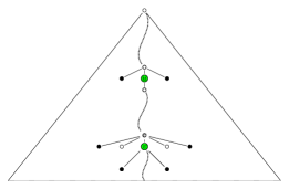
Figure 1: Naive combination of full types

Let $\varphi$ be a formula saying that every green vertex has at most three direct black neighbors below, on the left or on the right; formally

$$\varphi=\forall x\exists^{\leq 3}y\ \mathit{green}(x)\Rightarrow\left(\mathit{black}(y)\wedge\left(x\downarrow y\vee y\downarrow x\vee x\rightarrow y\vee y\rightarrow x\right)\right).$$

Let ${\mathfrak{T}}$ be a tree model from Fig. 1. Denote $\overline{\alpha}={\rm ftp}^{{\mathfrak{T}}}_{C(\varphi)}({u})$ and $\overline{\beta}={\rm ftp}^{{\mathfrak{T}}}_{C(\varphi)}({v})$. Because ${\mathfrak{T}}\models\varphi$, the $C(\varphi)$-full types $\overline{\alpha}$ and $\overline{\beta}$ are $\varphi$-consistent. However the combined $C(\varphi)$-full type $\overline{\gamma}$, in form described in Lemma 9, is not $\varphi$-consistent (the black nodes appear in $\overline{\gamma}$ on positions $\theta_{\downarrow}$, $\theta_{\leftarrow}$, $\theta_{\rightarrow}$ four times in total).

4.3 Small model theorem

The general scheme of the decidability proof of finite satisfiability of $\mbox{$\mbox{\rm C}^{2}$}[{\downarrow},{\downarrow^{\scriptscriptstyle+}},{\rightarrow},{\rightarrow^{\scriptscriptstyle+}}]$ is similar to the one from Section 3. Namely, we demonstrate the small-model property of the logic, showing that every satisfiable formula $\varphi$ has a tree model of depth and degree bounded exponentially in $|\varphi|$. It is also obtained in a similar way, by first shortening ${\downarrow}$-paths and then shortening the ${\rightarrow}$-paths. The technical details differ however.

Recall that given a normal form $\varphi$ we denote by $m$ the number of its $\forall\exists$ conjuncts, and by $\mbox{\large\boldmath$\alpha$}_{\varphi}$ the set of $1$-types over the signature consisting of the symbols appearing in $\varphi$.

Theorem 3 (Small model theorem).

Let $\varphi$ be a formula of $\mbox{$\mbox{\rm C}^{2}$}[{\downarrow},{\downarrow^{\scriptscriptstyle+}},{\rightarrow},{\rightarrow^{\scriptscriptstyle+}}]$ in normal form If $\varphi$ is satisfiable then it has a a tree model in which every path has length bounded by $3\cdot\left(C(\varphi)+2\right)^{10m+1}\cdot|\mbox{\large\boldmath$\alpha$}_{\varphi}|^{2}$ and every vertex has degree bounded by $(4C(\varphi)^{2}+8C(\varphi))\cdot|\mbox{\large\boldmath$\alpha$}_{\varphi}|^{5}$.

We split the proof of this theorem into two parts. In Section 4.3.1 we show how to reduce the length of paths in a tree and in Section 4.3.2 we show how to reduce the degree of every vertex.

4.3.1 Short paths

Lemma 10 (Cutting lemma).

Let $\varphi\in\mbox{$\mbox{$\mbox{\rm C}^{2}$}[{\downarrow},{\downarrow^{\scriptscriptstyle+}},{\rightarrow},{\rightarrow^{\scriptscriptstyle+}}]$}$ be a formula in normal form and ${\mathfrak{T}}$ be its tree model. If there are two vertices $u,v\in T$, such that $v$ is below $u$ and ${\rm rftp}^{{\mathfrak{T}}}_{\varphi}({u})={\rm rftp}^{{\mathfrak{T}}}_{\varphi}({v})$, then the tree ${\mathfrak{T}}^{\prime}$, obtained by replacing the subtree rooted at $u$ by the subtree rooted at $v$, is also a model of $\varphi$.

Proof.

The proof goes by case analysis. First, observe that the $C(\varphi)$-full type of $u$ in tree ${\mathfrak{T}}^{\prime}$ is a combination of the $C(\varphi)$-full types of $u$ and $v$ in ${\mathfrak{T}}$ and thus, by Lemma 9, it is $\varphi$-consistent. In the rest of the proof we show that for every vertex $w$ in ${\mathfrak{T}}^{\prime}$ we have ${\rm ftp}^{{\mathfrak{{T}}}}_{C(\varphi)}({w})={\rm ftp}^{{\mathfrak{{T}^{\prime}}}}_{C(\varphi)}({w})$. Then Lemma 8 guarantees that the obtained tree ${\mathfrak{T}}^{\prime}$ is indeed a model of $\varphi$.

Let $w$ be any vertex from $T^{\prime}$, or equivalently, a vertex from $T$ such that $w$ lies inside the tree rooted at $v$ or lies outside of the tree rooted at $u$. There are four possible ”locations” for $w$:

1. $w$ is above $u$ (cf. Fig. 2)

2. $w$ is below $v$ (cf. Fig. 3)

3. $w$ is in a free position to $u$ (cf. Fig. 4)

4. $w$ is a sibling of $u$

For the rest of the proof, denote $\overline{\alpha}={\rm ftp}^{{\mathfrak{{\mathfrak{T}}}}}_{C(\varphi)}({w})$ and $\overline{\beta}={\rm ftp}^{{\mathfrak{{\mathfrak{T}}^{\prime}}}}_{C(\varphi)}({w})$. Let us consider the four cases distinguished above.

1. $w$ is above $u$

   

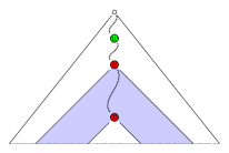
   Figure 2: Case (a)

   Of course cutting vertices between $u$ and $v$ does not change anything above or in free position to $w$, so obviously for all $\theta\in\{\theta_{=},\theta_{\uparrow},\theta_{\uparrow\uparrow^{+}},\theta_{\leftarrow},\theta_{\leftleftarrows^{+}},\theta_{\rightarrow},\theta_{\rightrightarrows^{+}},\theta_{\not\sim}\}$ we have $\overline{\alpha}(\theta){=}\overline{\beta}(\theta)$. The 1-type of the node immediately below $w$ is also not changed, so $\overline{\alpha}(\theta_{\downarrow})=\overline{\beta}(\theta_{\downarrow})$. The only missing case is equality of multisets $\overline{\alpha}(\theta_{\downarrow\downarrow^{+}})$ and $\overline{\beta}(\theta_{\downarrow\downarrow^{+}})$, but it follows from the equality of the $\varphi$-reduced types ${\rm rftp}^{{\mathfrak{T}}}_{\varphi}({u})$ and ${\rm rftp}^{{\mathfrak{T}}}_{\varphi}({v})$, and in particular their $B$-components. More specifically, for a given 1-type $\gamma$, the number of occurrences of $\gamma$ in $\overline{\alpha}(\theta_{\downarrow\downarrow^{+}})$ is (counted up to $C(\varphi)$) the number of occurrences of $\gamma$ in the subtree of ${\mathfrak{T}}$ rooted at $w$. We can divide this tree into three pieces, as in Fig. 2: the upper part without the subtree rooted at $u$, the lower part rooted at $v$ and the remaining middle part. Now, the multiplicity of $\gamma$ in $\overline{\alpha}(\theta_{\downarrow\downarrow^{+}})$ is simply the sum of multiplicities of $\gamma$ in each of these parts. But from the fact that ${\rm rftp}^{{\mathfrak{T}}}_{\varphi}({u})={\rm rftp}^{{\mathfrak{T}}}_{\varphi}({v})$, we know that the multiplicity of $\gamma$ in the subtree rooted at $u$ is the same as in the subtree rooted at $v$. It means that either there are more than $C(\varphi)$ occurrences of $\gamma$ in the subtree rooted at $v$ or there are no occurrences of $\gamma$ in the middle part. In both cases the multiplicity of $\gamma$ below $w$ is the same before and after the surgery.

2. $w$ is below $v$

   

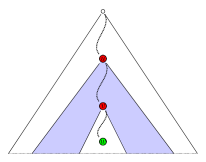
   Figure 3: Case (b)

   The reasoning to show that $\overline{\alpha}(\theta)=\overline{\beta}(\theta)$ for $\theta\in\{\theta_{=},\theta_{\uparrow},\theta_{\uparrow\uparrow^{+}},\theta_{\leftarrow},\theta_{\leftleftarrows^{+}},\theta_{\rightarrow},\theta_{\rightrightarrows^{+}},\theta_{\downarrow\downarrow^{+}}\}$ is the same or symmetric to the previous case.

   It is a bit more tricky to prove that $\overline{\alpha}(\theta_{\not\sim})=\overline{\beta}(\theta_{\not\sim})$. Consider an arbitrary 1-type $\gamma$. Observe that vertices of type $\gamma$ in free position to $w$ in ${\mathfrak{T}}$ are vertices of type $\gamma$ that are

   • in free position to $w$ in the subtree rooted at $v$ (denote the number of them by $\#w_{\not\sim}$),

   • close and distant siblings of $v$ (denoted $\#v_{\rightleftarrows}$),

   • vertices in free position to $v$ in the subtree rooted at $u$ (denoted $\#v_{\not\sim}$),

   • close and distant siblings of $u$ (denoted $\#u_{\rightleftarrows}$), or

   • in free position to $u$ in the whole tree ($\#u_{\not\sim}$).

   This gives us the equation:

   $$\left(\overline{\alpha}(\theta_{\not\sim})\right)\left(\gamma\right)=\mathit{cut}_{C(\varphi)}\left(\#w_{\not\sim}{+}\#v_{\rightleftarrows}{+}\#v_{\not\sim}{+}\#u_{\rightleftarrows}{+}\#u_{\not\sim}\right).$$

   By the assumption that ${\rm rftp}^{{\mathfrak{T}}}_{\varphi}({v})={\rm rftp}^{{\mathfrak{T}}}_{\varphi}({u})$, the $F$-components of these $\varphi$-reduced $C(\varphi)$-full types are equal, so $\mathit{cut}_{C(\varphi)}\left(\#v_{\rightleftarrows}{+}\#v_{\not\sim}{+}\#u_{\rightleftarrows}{+}\#u_{\not\sim}\right)=\mathit{cut}_{C(\varphi)}\left(\#v_{\rightleftarrows}{+}\#v_{\not\sim}\right)$. It means that either $\mathit{cut}_{C(\varphi)}\left(\#u_{\rightleftarrows}{+}\#u_{\not\sim}\right)=\infty$ or $\#v_{\rightleftarrows}+\#v_{\not\sim}=0$. In both cases, $\overline{\alpha}(\theta_{\not\sim})$ does not change after removing vertices between nodes $u$ and $v$.

3. $w$ is in a free position to $u$

   

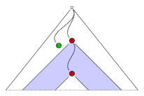
   Figure 4: Case (c)

   The fact that $\overline{\alpha}(\theta)=\overline{\beta}(\theta)$ for $\theta\in\{\theta_{\downarrow},\theta_{\downarrow\downarrow^{+}},\theta_{\leftarrow},\theta_{\leftleftarrows^{+}},\theta_{\rightarrow},\theta_{\rightrightarrows^{+}},\theta_{\uparrow},\theta_{\uparrow\uparrow^{+}},\theta_{=}\}$ is quite obvious (for the same reason as in the previous cases).

   We will show that $\overline{\alpha}(\theta_{\not\sim})=\overline{\beta}(\theta_{\not\sim})$. Observe that the whole tree rooted at $u$ is in free position to $w$. $C(\varphi)$-full types of all vertices $w^{\prime}$ outside this tree, such that ${\mathfrak{T}}\models\theta_{\not\sim}[w,w^{\prime}]$ don’t change, so we can concentrate only on vertices from that tree. Note that ${\rm rftp}^{{\mathfrak{T}}}_{\varphi}({u})={\rm rftp}^{{\mathfrak{T}}}_{\varphi}({v})$, which means equality of ”below” multisets. Because multiplicity of each $1$-type $\gamma$ below $v$ is equal to the multiplicity of $\gamma$ below $u$, we have equal multiplicity of vertices in free position to $w$ before and after replacing the root.

4. $w$ is a sibling of $u$

   The proof is similar to the previous ones. We only need to show that $\overline{\alpha}(\theta_{\not\sim})=\overline{\beta}(\theta_{\not\sim})$. Observe that ${\rm ftp}^{{\mathfrak{{T}}}}_{C(\varphi)}({u})(\theta_{\downarrow})\ \cup\ {\rm ftp}^{{\mathfrak{{T}}}}_{C(\varphi)}({u})(\theta_{\downarrow\downarrow^{+}})={\rm ftp}^{{\mathfrak{{T}}}}_{C(\varphi)}({v})(\theta_{\downarrow})\ \cup\ {\rm ftp}^{{\mathfrak{{T}}}}_{C(\varphi)}({v})(\theta_{\downarrow\downarrow^{+}})$, so we don’t accidentally cut any of the free witnesses of $w$, which proves the desired equality.

∎

Lemma 11.

Let $\varphi$ be a formula in normal form of $\mbox{$\mbox{\rm C}^{2}$}[{\downarrow},{\downarrow^{\scriptscriptstyle+}},{\rightarrow},{\rightarrow^{\scriptscriptstyle+}}]$ satisfied in a finite tree. Then there exists a tree model of $\varphi$ whose every $\downarrow$-path has length bounded by $3\cdot\left(C(\varphi)+2\right)^{10m+1}\cdot|\mbox{\large\boldmath$\alpha$}_{\varphi}|^{2}$.

Proof.

According to Lemma 10 we can restrict attention to models with the property that every $\varphi$-reduced full type appears only once on every $\downarrow$-path. Let ${\mathfrak{T}}\models\varphi$ be a tree model with this property. Let $v_{1},v_{2},\ldots,v_{n}$ be a $\downarrow$-path in ${\mathfrak{T}}$. Observe that the $\varphi$-reduced full types on this path behave in a monotonic way in the sense that for every $i$ and the $\varphi$-reduced full types of the $i,(i{+}1)$-th vertices $R_{i}=(\alpha_{i},W_{i},A_{i},B_{i},F_{i})$ and $R_{i+1}=(\alpha_{i+1},W_{i+1},A_{i+1},B_{i+1},F_{i+1})$, we have $A_{i}{\subseteq}A_{i+1},B_{i+1}{\subseteq}B_{i}$ and $F_{i}{\subseteq}F_{i+1}$. A $1$-type $\alpha$ can occur in a multiset from $0$ to $C(\varphi)$ times. If $\alpha$ appears more than $C(\varphi)$ times, its multiplicity is $\infty$. Hence the number of modifications of each multiset from $A,B,F$ is bounded by $\left(C(\varphi)+2\right)\cdot|\mbox{\large\boldmath$\alpha$}_{\varphi}|$. There are up to $|\mbox{\large\boldmath$\alpha$}_{\varphi}|\cdot(C(\varphi)+2)^{10m}$ $\varphi$-reduced full types with fixed multisets $A,B,F$ (because it is the number of all possible $1$-types multiplied by the number of all possible witness-counting functions). Combination of these two observations gives us the desired estimation $\left(C(\varphi)+2\right)^{10m+1}\cdot|\mbox{\large\boldmath$\alpha$}_{\varphi}|^{2}\cdot 3$. ∎

4.3.2 Small degree

Definition 8.

For a given vertex $v\in T$ and its $C(\varphi)$-full type ${\rm ftp}^{{\mathfrak{T}}}_{C(\varphi)}({v})=\overline{\alpha}$, the horizontal $C(\varphi)$-full type of $v$ in ${\mathfrak{T}}$ is the quintuple

$${\rm hftp}^{{\mathfrak{{\mathfrak{T}}}}}_{C(\varphi)}({v})=\left(\overline{\alpha}(\theta_{=}),\ \overline{\alpha}(\theta_{\rightarrow}),\ \overline{\alpha}(\theta_{\rightrightarrows^{+}}),\ \overline{\alpha}(\theta_{\leftarrow}),\ \overline{\alpha}(\theta_{\leftleftarrows^{+}})\right).$$

Lemma 12.

Let $\varphi$ be a formula in normal form of $\mbox{$\mbox{\rm C}^{2}$}[{\downarrow},{\downarrow^{\scriptscriptstyle+}},{\rightarrow},{\rightarrow^{\scriptscriptstyle+}}]$ satisfied in a finite tree ${\mathfrak{T}}$. Then there exists a tree model of $\varphi$, obtained by removing some subtrees from ${\mathfrak{T}}$, such that the degree of every vertex is bounded by $(4C(\varphi)^{2}+8C(\varphi))\cdot|\mbox{\large\boldmath$\alpha$}_{\varphi}|^{5}$.

Proof.

First, we will show how to limit the degree of a single vertex. After that we can traverse the tree in depth-first manner and, by cutting unwanted vertices, obtain the desired model. Let $v$ be a vertex from $T$. We denote by $\mathit{Children}(v)$ the set $\{u_{1},u_{2},\ldots,u_{N}\}$ of all children of $v$ (ordered by $\rightarrow_{+}$). For every $1$-type $\alpha$, we are going to mark some elements of $\mathit{Children}(v)$ and, after that, limit number of vertices between two adjacent marked ones.

Let $U_{\alpha}=\{u_{i}\mid{\rm tp}^{{\mathfrak{{T}}}}({u_{i}})=\alpha\}$ be the set of children of $v$ with the $1$-type $\alpha$ and let $U_{\alpha}^{\downarrow}=\{u_{i}\mid\exists w{\in}T\left(u_{i}{\downarrow}w\vee u_{i}{\downarrow\downarrow^{+}}w\right)\wedge{\rm tp}^{{\mathfrak{{T}}}}({w})=\alpha\}$ be the set of children of $v$ with descendants of $1$-type $\alpha$. For every $1$-type $\alpha$, we mark $\min\left(C(\varphi),|U_{\alpha}|\right)$ vertices from $U_{\alpha}$ and $\min(C(\varphi),|U_{\alpha}^{\downarrow}|)$ vertices from $U_{\alpha}^{\downarrow}$ (it is important to mark $u_{1}$ and $u_{N}$ during this process). Marked vertices are the required witnesses for vertex $v$. The number of marked vertices ensure us that during the cutting we don’t loose also any of free witnesses for any other vertex in the tree ${\mathfrak{T}}$. It’s easy to see that during this process we marked at most $2C(\varphi)\cdot|\mbox{\large\boldmath$\alpha$}_{\varphi}|$ vertices.

Now the reasoning is similar to that of Lemma 10. Let $u_{i},u_{j}$ (where $i<j$) be two unmarked vertices, such that their horizontal $C(\varphi)$-full types are the same (${\rm hftp}^{{\mathfrak{{\mathfrak{T}}}}}_{C(\varphi)}({u_{i}})={\rm hftp}^{{\mathfrak{{\mathfrak{T}}}}}_{C(\varphi)}({u_{j}})$) and there are no marked vertices between them. Then the tree obtained by removing all vertices between $u_{i}$ and $u_{j}$, including $u_{i}$ and excluding $u_{j}$, together with subtrees rooted at them, is also a model of $\varphi$. To prove it, first observe that cutting the vertices between $u_{i}$ and $u_{j}$ does not change any of vertices above and below $u_{i}$ and $u_{j}$. The marked vertices guarantee that none of vertices in the whole tree lost its free witnesses. Equality of the horizontal $C(\varphi)$-full types of $u_{i}$ and $u_{j}$ ensures that the numbers of right and left witnesses for vertices $u_{i}$ and $u_{j}$ are correct. Therefore the combined $C(\varphi)$-full type of $u_{j}$, realized in the tree after the surgery, is $\varphi$-consistent. By Lemma 8, the obtained tree is a model for the formula $\varphi$.

Continuing this process we can remove all vertices between the marked pairs with the same horizontal $C(\varphi)$-full types. Observe that $\theta_{\rightrightarrows^{+}}$ and $\theta_{\leftleftarrows^{+}}$ components of the horizontal $C(\varphi)$-full types behave in the monotonic way. For fixed $\theta_{\leftarrow},\theta_{\rightarrow},\theta_{=}$ components of a given horizontal $C(\varphi)$-full type, the number of its possible modifications on the path is bounded by $2\cdot(C(\varphi)+2)\cdot|\mbox{\large\boldmath$\alpha$}_{\varphi}|$. This guarantees that between any adjacent marked vertices, we have at most $|\mbox{\large\boldmath$\alpha$}_{\varphi}|^{3}\cdot 2(C(\varphi)+2)\cdot|\mbox{\large\boldmath$\alpha$}_{\varphi}|$ vertices. Using the fact that we marked at most $2C(\varphi)\cdot|\mbox{\large\boldmath$\alpha$}_{\varphi}|$ vertices and we know the upper bound on lengths of paths between adjacent marked vertices, we can reduce the number of children of $v$ to $(4C(\varphi)^{2}+8C(\varphi))\cdot|\mbox{\large\boldmath$\alpha$}_{\varphi}|^{5}$.

By repeating this procedure as long as there are vertices of high degree we obtain a desired model of $\varphi$. ∎

4.4 Algorithm

In this section we design an algorithm checking if a given formula $\varphi\in\mbox{$\mbox{$\mbox{\rm C}^{2}$}[{\downarrow},{\downarrow^{\scriptscriptstyle+}},{\rightarrow},{\rightarrow^{\scriptscriptstyle+}}]$}$ has a finite tree model. First, by Lemma 2, we can assume that $\varphi$ is in normal form. Second, by Theorem 3, we can restrict attention to models with exponentially bounded vertex degree and $\downarrow$-path length.

We will present an alternating algorithm working in exponential space. The idea of the algorithm is quite simple. For each vertex $v$ we will guess its $C(\varphi)$-full type and check if it is $\varphi$-consistent. If it is, we guess the $v$’s children and their full types. After that, we check if their $C(\varphi)$-full types are locally consistent (see the procedure below), which guarantees that we guessed correctly. The algorithm starts with $v=$ root and works recursively with its children. The procedure presented here is a modification of the one from [5].

Procedure 1 Checking if given $C(\varphi)$-full types are locally-consistent

0:  $C(\varphi)$-Full types $\overline{\alpha}$, $\overline{\alpha_{1}}$, $\ldots$, $\overline{\alpha_{k}}$

1:  Return True if all of the statements below are true. Return False otherwise.

2:  $\overline{\alpha_{i}}(\theta_{\leftarrow})=\overline{\alpha_{i-1}}(\theta_{=})$ for $i>1$ and $\overline{\alpha_{1}}(\theta_{\leftarrow})=\emptyset$

3:  $\overline{\alpha_{i}}(\theta_{\leftleftarrows^{+}})=\overline{\alpha_{i-1}}(\theta_{\leftarrow})\cup\overline{\alpha_{i-1}}(\theta_{\leftleftarrows^{+}})$ for $i>1$ and $\overline{\alpha_{1}}(\theta_{\leftleftarrows^{+}})=\emptyset$

4:  $\overline{\alpha_{i}}(\theta_{\rightarrow})=\overline{\alpha_{i+1}}(\theta_{=})$ for $i<k$ and $\overline{\alpha_{k}}(\theta_{\rightarrow})=\emptyset$

5:  $\overline{\alpha_{i}}(\theta_{\rightrightarrows^{+}})=\overline{\alpha_{i+1}}(\theta_{\rightarrow})\cup\overline{\alpha_{i+1}}(\theta_{\rightrightarrows^{+}})$ for $i<k$ and $\overline{\alpha_{k}}(\theta_{\rightrightarrows^{+}})=\emptyset$

6:  $\overline{\alpha}(\theta_{\downarrow})=\bigcup_{j=1}^{k}\overline{\alpha_{j}}(\theta_{=})$

7:  $\overline{\alpha}(\theta_{\downarrow\downarrow^{+}})=\bigcup_{i=1}^{k}\left(\overline{\alpha_{i}}(\theta_{\downarrow})\cup\overline{\alpha_{i}}(\theta_{\downarrow\downarrow^{+}})\right)$

8:  for $1\leq i\leq k:$ $\overline{\alpha_{i}}(\theta_{\uparrow})=\overline{\alpha}(\theta_{=})$

9:  for $1\leq i\leq k:$$\overline{\alpha_{i}}(\theta_{\not\sim})=\overline{\alpha}(\theta_{\not\sim})\cup\overline{\alpha}(\theta_{\leftarrow})\cup\overline{\alpha}(\theta_{\rightarrow})\cup\overline{\alpha}(\theta_{\leftleftarrows^{+}})\cup\overline{\alpha}(\theta_{\rightrightarrows^{+}})\cup\bigcup_{j\neq i}\left(\overline{\alpha_{j}}(\theta_{\downarrow})\cup\overline{\alpha_{j}}(\theta_{\downarrow\downarrow^{+}})\right)$

Procedure 2 Satisfiability test for $\mbox{$\mbox{\rm C}^{2}$}[{\downarrow},{\downarrow^{\scriptscriptstyle+}},{\rightarrow},{\rightarrow^{\scriptscriptstyle+}}]$

0:  Formula $\varphi\in\mbox{$\mbox{$\mbox{\rm C}^{2}$}[{\downarrow},{\downarrow^{\scriptscriptstyle+}},{\rightarrow},{\rightarrow^{\scriptscriptstyle+}}]$}$ in normal form.

1:  Let MaxDepth := $3\cdot\left(C(\varphi)+2\right)^{10m+1}\cdot|\mbox{\large\boldmath$\alpha$}_{\varphi}|^{2}$

2:  Let MaxDeg := $(4C(\varphi)^{2}+8C(\varphi))\cdot|\mbox{\large\boldmath$\alpha$}_{\varphi}|^{5}$

3:  Lvl := $0$.

4:  guess a $C(\varphi)$-full type $\overline{\alpha}$ s.t. $\overline{\alpha}(\theta)=\emptyset$ for $\theta\in\{\theta_{\uparrow},\theta_{\uparrow\uparrow^{+}},\theta_{\rightarrow},\theta_{\leftarrow},\theta_{\rightrightarrows^{+}},\theta_{\leftleftarrows^{+}},\theta_{\not\sim}\}$.

5:  while Lvl $<$ MaxDepth  do

6:     if $\overline{\alpha}$ is not $\varphi$-consistent then reject

7:     if $\overline{\alpha}(\theta_{\downarrow})=\overline{\alpha}(\theta_{\downarrow\downarrow^{+}})=\emptyset$ then accept

8:     guess an integer $1\leq k\leq$ MaxDeg

9:     guess $C(\varphi)$-full types $\overline{\alpha_{1}}$, $\overline{\alpha_{2}}$, $\ldots$, $\overline{\alpha_{k}}$

10:     if not locally-consistent$\left(\overline{\alpha},\overline{\alpha_{1}},\overline{\alpha_{2}},\ldots,\overline{\alpha_{k}}\right)$ then reject

11:     Lvl $:=$ Lvl $+$ $1$

12:     universally choose $1\leq i\leq k$; let $\overline{\alpha}=\overline{\alpha_{i}}$

13:  reject

Lemma 13.

Procedure 2 accepts its input $\varphi$ iff $\varphi$ is satisfiable.

Proof.

Assume $\varphi$ is satisfiable. Then there exists a small tree model ${\mathfrak{T}}$ as guaranteed by Theorem 3. We can run the algorithm and guess exactly the same $C(\varphi)$-full types as in ${\mathfrak{T}}$. The guessed $C(\varphi)$-full types are locally-consistent and $\varphi$-consistent, so procedure 2 accepts.

Assume that Procedure 2 accepts its input $\varphi$. Then we can reconstruct the tree ${\mathfrak{T}}$ from the received $C(\varphi)$-full types. The guessed $C(\varphi)$-full types are $\varphi$-consistent, which guarantees that we have the right number of witnesses to satisfy the formula. Moreover, the function locally-consistent ensures that the $C(\varphi)$-full types realized in ${\mathfrak{T}}$ are indeed as we guessed. By Lemma 8, ${\mathfrak{T}}$ is a tree model for $\varphi$ and thus $\varphi$ is satisfiable.

∎

Theorem 4.

The satisfiability problem for $\mbox{$\mbox{\rm C}^{2}$}[{\downarrow},{\downarrow^{\scriptscriptstyle+}},{\rightarrow},{\rightarrow^{\scriptscriptstyle+}}]$ over finite trees is ExpSpace-complete.

Proof.

Our procedure works in alternating exponential time, since maximum degree and path length are bounded exponentially in $|\varphi|$. The ExpSpace-upper bound follows from the well know fact that AExpTime=ExpSpace. The ExpSpace-lower bound comes from [2]. ∎

5 Expressive power

A natural question is whether adding counting quantifiers increases the expressive power of two-variable logic over trees. We answer this question concentrating on the classical scenario assuming that signatures contain no common binary symbols. Under this scenario $\mathrm{FO}^{2}$$[{\downarrow},{\downarrow^{\scriptscriptstyle+}},{\rightarrow},{\rightarrow^{\scriptscriptstyle+}}]$ is known to be expressively equivalent to the navigational core of XPath [20]. Here we show that $\mbox{\rm C}^{2}$$[{\downarrow},{\downarrow^{\scriptscriptstyle+}},{\rightarrow},{\rightarrow^{\scriptscriptstyle+}}]$ shares the same expressivity.

Let us note, however, that it is the presence of the sibling relations which makes $\mathrm{FO}^{2}$ and $\mbox{\rm C}^{2}$ equivalent. Indeed, over unordered trees $\mathrm{FO}^{2}$ cannot count:

Theorem 5.

$\mathrm{FO}^{2}$$[{\downarrow},{\downarrow^{\scriptscriptstyle+}}]$ is less expressive than $\mbox{\rm C}^{2}$$[{\downarrow},{\downarrow^{\scriptscriptstyle+}}]$.

Proof.

Let us assume that the signature contains no unary predicates and for $i\in{\mathbb{N}}$ let ${\mathfrak{T}}_{i}$ denote the tree consisting just of a root and its $i$ children. Obviously ${\mathfrak{T}}_{3}\models\exists x\exists^{\geq 3}y\;x{\downarrow^{\scriptscriptstyle+}}y$ while ${\mathfrak{T}}_{2}\not\models\exists x\exists^{\geq 3}y\;x{\downarrow^{\scriptscriptstyle+}}y$. On the other hand, ${\mathfrak{T}}_{2}$ and ${\mathfrak{T}}_{3}$ are indistinguishable in $\mathrm{FO}^{2}$$[{\downarrow},{\downarrow^{\scriptscriptstyle+}}]$. It can be seen by observing that Duplicator has a simple winning strategy in the standard two-pebble game of any length played on ${\mathfrak{T}}_{2}$ and ${\mathfrak{T}}_{3}$. ∎

Now we turn to the advertised equivalence of $\mathrm{FO}^{2}$ and $\mbox{\rm C}^{2}$ in the case of full navigational signature.

Theorem 6.

$\mathrm{FO}^{2}$$[{\downarrow},{\downarrow^{\scriptscriptstyle+}},{\rightarrow},{\rightarrow^{\scriptscriptstyle+}}]$ and $\mbox{\rm C}^{2}$$[{\downarrow},{\downarrow^{\scriptscriptstyle+}},{\rightarrow},{\rightarrow^{\scriptscriptstyle+}}]$ are expressively equivalent.

We give a detailed proof. First we show that one can say in $\mathrm{FO}^{2}$$[{\downarrow},{\downarrow^{\scriptscriptstyle+}},{\rightarrow},{\rightarrow^{\scriptscriptstyle+}}]$ that for a given node $v$ there are at least $k$ nodes in some specific position to $v$ that have a fixed unary property $\psi$ expressible in $\mathrm{FO}^{2}$. Let us define the set $\cal P$ of positions we are interested in. Some of the positions correspond directly to the order formulas from $\Theta$, but for technical reasons we need to introduce also some other. We represent the positions with help of graphical symbols. Intuitively, the crossed circle corresponds to $v$, the filled circles correspond to nodes among which we look for those satisfying $\psi$ and the empty circles are auxiliary. We distinguish sixteen positions:

${\cal P}=\{\scalebox{0.8}{ \leavevmode\hbox to17.46pt{\vbox to25.03pt{\text{[drawing]}}} },\scalebox{0.8}{ \leavevmode\hbox to17.46pt{\vbox to25.03pt{\text{[drawing]}}} },\scalebox{0.8}{ \leavevmode\hbox to30.26pt{\vbox to27.63pt{\text{[drawing]}}} },\scalebox{0.8}{ \leavevmode\hbox to30.26pt{\vbox to27.63pt{\text{[drawing]}}} },\scalebox{0.8}{ \leavevmode\hbox to25.86pt{\vbox to27.63pt{\text{[drawing]}}} },\scalebox{0.8}{ \leavevmode\hbox to25.86pt{\vbox to27.63pt{\text{[drawing]}}} },\scalebox{0.8}{ \leavevmode\hbox to14.44pt{\vbox to25.03pt{\text{[drawing]}}} },\scalebox{0.8}{ \leavevmode\hbox to18.45pt{\vbox to25.03pt{\text{[drawing]}}} },\scalebox{0.8}{ \leavevmode\hbox to17.46pt{\vbox to25.03pt{\text{[drawing]}}} },\scalebox{0.8}{ \leavevmode\hbox to18.45pt{\vbox to25.03pt{\text{[drawing]}}} },\scalebox{0.8}{ \leavevmode\hbox to25.86pt{\vbox to16.17pt{\text{[drawing]}}} },\scalebox{0.8}{ \leavevmode\hbox to25.86pt{\vbox to16.17pt{\text{[drawing]}}} }\\$ $\hskip 250.0pt\scalebox{0.8}{ \leavevmode\hbox to25.86pt{\vbox to16.17pt{\text{[drawing]}}} },\scalebox{0.8}{ \leavevmode\hbox to25.86pt{\vbox to16.17pt{\text{[drawing]}}} },\scalebox{0.8}{ \leavevmode\hbox to41.67pt{\vbox to27.63pt{\text{[drawing]}}} },\scalebox{0.8}{ \leavevmode\hbox to41.67pt{\vbox to28.74pt{\text{[drawing]}}} }\}.$

Let us formalize the given intuitive meaning of the introduced symbols. Let ${\mathfrak{T}}$ be a tree, $v$ its node, $c$ a natural number, $pos\in{\cal P}$, and $\psi$ any $\mathrm{FO}^{2}$$[{\downarrow},{\downarrow^{\scriptscriptstyle+}},{\rightarrow},{\rightarrow^{\scriptscriptstyle+}}]$ formula with one free variable, We say that $v$ satisfies property $W\left\langle c,pos,\psi\right\rangle$ if there are at least $c$ nodes $w$ such that ${\mathfrak{T}}\models\psi[w]$ and $w$ is in position $pos$ to $v$, i.e.,

• if $pos=\scalebox{0.8}{ \leavevmode\hbox to17.46pt{\vbox to25.03pt{\text{[drawing]}}} }$ then $w$ is a descendant of $v$,

• if $pos=\scalebox{0.8}{ \leavevmode\hbox to17.46pt{\vbox to25.03pt{\text{[drawing]}}} }$ then $w=v$ or $w$ is a descendant of $v$,

• if $pos=\scalebox{0.8}{ \leavevmode\hbox to30.26pt{\vbox to27.63pt{\text{[drawing]}}} }$ then $w$ is a following-sibling of $v$ or a descendant of a following-sibling of $v$,

• if $pos=\scalebox{0.8}{ \leavevmode\hbox to30.26pt{\vbox to27.63pt{\text{[drawing]}}} }$ then $w$ is a descendant of a following-sibling of $v$,

• if $pos=\scalebox{0.8}{ \leavevmode\hbox to25.86pt{\vbox to27.63pt{\text{[drawing]}}} }$ then $w$ is a preceding-sibling of $v$ or a descendant of a preceding-sibling of $v$,

• if $pos=\scalebox{0.8}{ \leavevmode\hbox to25.86pt{\vbox to27.63pt{\text{[drawing]}}} }$ then $w$ is a descendant of a preceding-sibling of $v$,

• if $pos=\scalebox{0.8}{ \leavevmode\hbox to14.44pt{\vbox to25.03pt{\text{[drawing]}}} }$ then $w$ is a child of $v$,

• if $pos=\scalebox{0.8}{ \leavevmode\hbox to18.45pt{\vbox to25.03pt{\text{[drawing]}}} }$ then $w$ is a descendant of $v$ but not its child,

• if $pos=\scalebox{0.8}{ \leavevmode\hbox to17.46pt{\vbox to25.03pt{\text{[drawing]}}} }$ then $w$ is an ancestor of $v$,

• if $pos=\scalebox{0.8}{ \leavevmode\hbox to18.45pt{\vbox to25.03pt{\text{[drawing]}}} }$ then $w$ is an ancestor of $v$ but not its father,

• if $pos=\scalebox{0.8}{ \leavevmode\hbox to25.86pt{\vbox to16.17pt{\text{[drawing]}}} }$ then $w$ is a following-sibling of $v$,

• if $pos=\scalebox{0.8}{ \leavevmode\hbox to25.86pt{\vbox to16.17pt{\text{[drawing]}}} }$ then $w$ is a preceding-sibling of $v$,

• if $pos=\scalebox{0.8}{ \leavevmode\hbox to25.86pt{\vbox to16.17pt{\text{[drawing]}}} }$ then $w$ is a following-sibling of $v$ but not the closest one,

• if $pos=\scalebox{0.8}{ \leavevmode\hbox to25.86pt{\vbox to16.17pt{\text{[drawing]}}} }$ then $w$ is a preceding-sibling of $v$ but not the closest one,

• if $pos=\scalebox{0.8}{ \leavevmode\hbox to41.67pt{\vbox to27.63pt{\text{[drawing]}}} }$ then $w$ is a sibling of $v$ or a descendant of a sibling of $v$,

• if $pos=\scalebox{0.8}{ \leavevmode\hbox to41.67pt{\vbox to28.74pt{\text{[drawing]}}} }$ then $w$ a sibling of an ancestor of $v$ or a descendant of a sibling of an ancestor of $v$.

Lemma 14.

For any $c\in{\mathbb{N}}$, any $\mathrm{FO}^{2}$$[{\downarrow},{\downarrow^{\scriptscriptstyle+}},{\rightarrow},{\rightarrow^{\scriptscriptstyle+}}]$ formula $\psi$ with one free variable, and $pos\in{\cal P}$, there is an $\mathrm{FO}^{2}$$[{\downarrow},{\downarrow^{\scriptscriptstyle+}},{\rightarrow},{\rightarrow^{\scriptscriptstyle+}}]$ formula $\Psi\langle c,pos,\psi\rangle$ with one free variable, such that for any tree ${\mathfrak{T}}$ and $v\in T$ we have ${\mathfrak{T}}\models\Psi\langle c,pos,\psi\rangle[v]$ iff $v$ satisfies $W\left\langle c,pos,\psi\right\rangle$.

Proof.

The proof goes by induction on $c$. The base case $c=1$ is straightforward:

• $\Psi\langle 1,\scalebox{0.8}{ \leavevmode\hbox to17.46pt{\vbox to25.03pt{\text{[drawing]}}} },\psi\rangle(x)\equiv\exists y\;(x{\downarrow^{\scriptscriptstyle+}}y\wedge\psi(y))$

• $\Psi\langle 1,\scalebox{0.8}{ \leavevmode\hbox to17.46pt{\vbox to25.03pt{\text{[drawing]}}} },\psi\rangle(x)\equiv\psi(x)\vee\exists y\;(x{\downarrow^{\scriptscriptstyle+}}y\wedge\psi(y))$

• $\Psi\langle 1,\scalebox{0.8}{ \leavevmode\hbox to30.26pt{\vbox to27.63pt{\text{[drawing]}}} },\psi\rangle(x)\equiv\exists y\;(x{\rightarrow^{\scriptscriptstyle+}}y\wedge\psi(y))\vee\exists y\;(x{\rightarrow^{\scriptscriptstyle+}}y\wedge\exists x(y{\downarrow^{\scriptscriptstyle+}}x\wedge\psi(x)))$

• $\Psi\langle 1,\scalebox{0.8}{ \leavevmode\hbox to30.26pt{\vbox to27.63pt{\text{[drawing]}}} },\psi\rangle(x)\equiv\exists y\;(x{\rightarrow^{\scriptscriptstyle+}}y\wedge\exists x(y{\downarrow^{\scriptscriptstyle+}}x\wedge\psi(x)))$

• $\Psi\langle 1,\scalebox{0.8}{ \leavevmode\hbox to25.86pt{\vbox to27.63pt{\text{[drawing]}}} },\psi\rangle(x)$ analogously

• $\Psi\langle 1,\scalebox{0.8}{ \leavevmode\hbox to25.86pt{\vbox to27.63pt{\text{[drawing]}}} },\psi\rangle(x)$ analogously

• $\Psi\langle 1,\scalebox{0.8}{ \leavevmode\hbox to14.44pt{\vbox to25.03pt{\text{[drawing]}}} },\psi\rangle(x)\equiv\exists y\;(x{\downarrow}y\wedge\psi(y))$

• $\Psi\langle 1,\scalebox{0.8}{ \leavevmode\hbox to18.45pt{\vbox to25.03pt{\text{[drawing]}}} },\psi\rangle(x)\equiv\exists y\;(x{\downarrow^{\scriptscriptstyle+}}y\wedge\neg(x{\downarrow}y)\wedge\psi(y))$

• $\Psi\langle 1,\scalebox{0.8}{ \leavevmode\hbox to17.46pt{\vbox to25.03pt{\text{[drawing]}}} },\psi\rangle(x)\equiv\exists y\;(y{\downarrow^{\scriptscriptstyle+}}x\wedge\psi(y))$

• $\Psi\langle 1,\scalebox{0.8}{ \leavevmode\hbox to18.45pt{\vbox to25.03pt{\text{[drawing]}}} },\psi\rangle(x)\equiv\exists y\;(y{\downarrow^{\scriptscriptstyle+}}x\wedge\neg(y{\downarrow}x)\wedge\psi(y))$

• $\Psi\langle 1,\scalebox{0.8}{ \leavevmode\hbox to25.86pt{\vbox to16.17pt{\text{[drawing]}}} },\psi\rangle(x)\equiv\exists y\;(x{\rightarrow^{\scriptscriptstyle+}}y\wedge\psi(y))$

• $\Psi\langle 1,\scalebox{0.8}{ \leavevmode\hbox to25.86pt{\vbox to16.17pt{\text{[drawing]}}} },\psi\rangle(x)$ analogously

• $\Psi\langle 1,\scalebox{0.8}{ \leavevmode\hbox to25.86pt{\vbox to16.17pt{\text{[drawing]}}} },\psi\rangle(x)\equiv\exists y\;(x{\rightarrow^{\scriptscriptstyle+}}y\wedge\neg(x{\downarrow}y)\wedge\psi(y))$

• $\Psi\langle 1,\scalebox{0.8}{ \leavevmode\hbox to25.86pt{\vbox to16.17pt{\text{[drawing]}}} },\psi\rangle(x)$ analogously

• $\Psi\langle 1,\scalebox{0.8}{ \leavevmode\hbox to41.67pt{\vbox to27.63pt{\text{[drawing]}}} },\psi\rangle(x)\equiv\exists y\;((x{\rightarrow^{\scriptscriptstyle+}}y\vee(y{\rightarrow^{\scriptscriptstyle+}}x)\wedge(\psi(y)\vee\exists x(y{\downarrow^{\scriptscriptstyle+}}x\wedge\psi(x)))$

• $\Psi\langle 1,\scalebox{0.8}{ \leavevmode\hbox to41.67pt{\vbox to28.74pt{\text{[drawing]}}} },\psi\rangle(x)\equiv\exists y\;(y{\downarrow^{\scriptscriptstyle+}}x\wedge\exists x((y{\rightarrow^{\scriptscriptstyle+}}x\vee x{\rightarrow^{\scriptscriptstyle+}}y)\wedge(\psi(x)\vee\exists y(x{\downarrow^{\scriptscriptstyle+}}y\wedge\psi(y)))))$

Assume now that the desired $\Psi\langle c,pos,\psi\rangle$ formulas exist for all $1\leq c<k$. We show how to define $\Psi\langle k,pos,\psi\rangle$ using $\Psi\langle c,pos^{\prime},\psi\rangle$ for $c<k$, or $c=k$ but in this case for $pos^{\prime}$ defined in one of the earlier items. If in any definition $\Psi\langle c,pos,\psi\rangle$ with $c=0$ appears it is replaced by $\top$.

• $\Psi\langle k,\scalebox{0.8}{ \leavevmode\hbox to17.46pt{\vbox to25.03pt{\text{[drawing]}}} },\psi\rangle(x)\equiv$
  $\exists y(x{\downarrow^{\scriptscriptstyle+}}y\wedge((\psi(y)\wedge\Psi\langle k-1,\scalebox{0.8}{ \leavevmode\hbox to17.46pt{\vbox to25.03pt{\text{[drawing]}}} },\psi\rangle(y))\vee\bigvee_{i\in[1,k-1]}(\Psi\langle i,\scalebox{0.8}{ \leavevmode\hbox to17.46pt{\vbox to25.03pt{\text{[drawing]}}} },\psi\rangle(y)\wedge\Psi\langle k-i,\scalebox{0.8}{ \leavevmode\hbox to30.26pt{\vbox to27.63pt{\text{[drawing]}}} },\psi\rangle(y)))$

• $\Psi\langle k,\scalebox{0.8}{ \leavevmode\hbox to17.46pt{\vbox to25.03pt{\text{[drawing]}}} },\psi\rangle(x)\equiv$ $\psi(x)\wedge\Psi\langle k-1,\scalebox{0.8}{ \leavevmode\hbox to17.46pt{\vbox to25.03pt{\text{[drawing]}}} },\psi\rangle(x)\vee\Psi\langle k,\scalebox{0.8}{ \leavevmode\hbox to17.46pt{\vbox to25.03pt{\text{[drawing]}}} },\psi\rangle(x)$

• $\Psi\langle k,\scalebox{0.8}{ \leavevmode\hbox to30.26pt{\vbox to27.63pt{\text{[drawing]}}} },\psi\rangle(x)\equiv$ $\exists y(x{\rightarrow^{\scriptscriptstyle+}}y\wedge\bigvee_{i\in[1,k]}(\Psi\langle i,\scalebox{0.8}{ \leavevmode\hbox to17.46pt{\vbox to25.03pt{\text{[drawing]}}} },\psi\rangle(y)\wedge\Psi\langle k-i,\scalebox{0.8}{ \leavevmode\hbox to30.26pt{\vbox to27.63pt{\text{[drawing]}}} },\psi\rangle(y)))$

• $\Psi\langle k,\scalebox{0.8}{ \leavevmode\hbox to30.26pt{\vbox to27.63pt{\text{[drawing]}}} },\psi\rangle(x)\equiv$ $\exists y(x{\rightarrow^{\scriptscriptstyle+}}y\wedge\bigvee_{i\in[1,k]}(\Psi\langle i,\scalebox{0.8}{ \leavevmode\hbox to17.46pt{\vbox to25.03pt{\text{[drawing]}}} },\psi\rangle(y)\wedge\Psi\langle k-i,\scalebox{0.8}{ \leavevmode\hbox to30.26pt{\vbox to27.63pt{\text{[drawing]}}} },\psi\rangle(y)))$

• $\Psi\langle k,\scalebox{0.8}{ \leavevmode\hbox to25.86pt{\vbox to27.63pt{\text{[drawing]}}} },\psi\rangle(x)$ analogously

• $\Psi\langle k,\scalebox{0.8}{ \leavevmode\hbox to25.86pt{\vbox to27.63pt{\text{[drawing]}}} },\psi\rangle(x)$ analogously

• $\Psi\langle k,\scalebox{0.8}{ \leavevmode\hbox to14.44pt{\vbox to25.03pt{\text{[drawing]}}} },\psi\rangle(x)\equiv$ $\exists y(x{\downarrow}y\wedge\psi(y)\wedge\Psi\langle k-1,\scalebox{0.8}{ \leavevmode\hbox to25.86pt{\vbox to16.17pt{\text{[drawing]}}} },\psi\rangle(y))$

• $\Psi\langle k,\scalebox{0.8}{ \leavevmode\hbox to18.45pt{\vbox to25.03pt{\text{[drawing]}}} },\psi\rangle(x)\equiv$ $\exists y(x{\downarrow}y\wedge\bigvee_{i\in[1,k]}(\Psi\langle i,\scalebox{0.8}{ \leavevmode\hbox to17.46pt{\vbox to25.03pt{\text{[drawing]}}} },\psi\rangle(y)\wedge\Psi\langle k-i,\scalebox{0.8}{ \leavevmode\hbox to30.26pt{\vbox to27.63pt{\text{[drawing]}}} },\psi\rangle(y)))$

• $\Psi\langle k,\scalebox{0.8}{ \leavevmode\hbox to17.46pt{\vbox to25.03pt{\text{[drawing]}}} },\psi\rangle(x)\equiv$ $\exists y(y{\downarrow^{\scriptscriptstyle+}}x\wedge\psi(y)\wedge\Psi\langle k-1,\scalebox{0.8}{ \leavevmode\hbox to17.46pt{\vbox to25.03pt{\text{[drawing]}}} },\psi\rangle(y))$

• $\Psi\langle k,\scalebox{0.8}{ \leavevmode\hbox to18.45pt{\vbox to25.03pt{\text{[drawing]}}} },\psi\rangle(x)\equiv$ $\exists y(y{\downarrow^{\scriptscriptstyle+}}x\wedge\neg(y{\downarrow}x)\wedge\psi(y)\wedge\Psi\langle k-1,\scalebox{0.8}{ \leavevmode\hbox to17.46pt{\vbox to25.03pt{\text{[drawing]}}} },\psi\rangle(y))$

• $\Psi\langle k,\scalebox{0.8}{ \leavevmode\hbox to25.86pt{\vbox to16.17pt{\text{[drawing]}}} },\psi\rangle(x)\equiv$ $\exists y(x{\rightarrow^{\scriptscriptstyle+}}y\wedge\psi(y)\wedge\Psi\langle k-1,\scalebox{0.8}{ \leavevmode\hbox to25.86pt{\vbox to16.17pt{\text{[drawing]}}} },\psi\rangle(y))$

• $\Psi\langle k,\scalebox{0.8}{ \leavevmode\hbox to25.86pt{\vbox to16.17pt{\text{[drawing]}}} },\psi\rangle(x)\equiv$ analogously

• $\Psi\langle k,\scalebox{0.8}{ \leavevmode\hbox to25.86pt{\vbox to16.17pt{\text{[drawing]}}} },\psi\rangle(x)\equiv$ $\exists y(x{\rightarrow^{\scriptscriptstyle+}}y\wedge\neg(x{\rightarrow}y)\wedge\psi(y)\wedge\Psi\langle k-1,\scalebox{0.8}{ \leavevmode\hbox to25.86pt{\vbox to16.17pt{\text{[drawing]}}} },\psi\rangle(y))$

• $\Psi\langle k,\scalebox{0.8}{ \leavevmode\hbox to25.86pt{\vbox to16.17pt{\text{[drawing]}}} },\psi\rangle\equiv$ analogously

• $\Psi\langle k,\scalebox{0.8}{ \leavevmode\hbox to41.67pt{\vbox to27.63pt{\text{[drawing]}}} },\psi\rangle\equiv$ $\bigvee_{i\in[0,k]}(\Psi\langle i,\scalebox{0.8}{ \leavevmode\hbox to30.26pt{\vbox to27.63pt{\text{[drawing]}}} },\psi\rangle(x)\wedge\Psi\langle k-i,\scalebox{0.8}{ \leavevmode\hbox to25.86pt{\vbox to27.63pt{\text{[drawing]}}} },\psi\rangle(x))$

• $\Psi\langle k,\scalebox{0.8}{ \leavevmode\hbox to41.67pt{\vbox to28.74pt{\text{[drawing]}}} },\psi\rangle\equiv$ $\exists y(y{\downarrow^{\scriptscriptstyle+}}x\wedge\bigvee_{i\in[1,k]}(\Psi\langle i,\scalebox{0.8}{ \leavevmode\hbox to41.67pt{\vbox to27.63pt{\text{[drawing]}}} },\psi\rangle(y)\wedge\Psi\langle k-i,\scalebox{0.8}{ \leavevmode\hbox to41.67pt{\vbox to28.74pt{\text{[drawing]}}} },\psi\rangle(y))).$

Most of the above equivalences are obvious. As an example, let us explain the first one. Assume that ${\mathfrak{T}}\models\Psi\langle k,\scalebox{0.8}{ \leavevmode\hbox to17.46pt{\vbox to25.03pt{\text{[drawing]}}} },\psi\rangle[v]$. Choose $k$ descendants of $v$ satisfying $\psi$. Let $u$ be the maximal element of ${\mathfrak{T}}$ such that all the chosen elements are in the subtree of $u$. If $u$ is one of the chosen elements then ${\mathfrak{T}}\models v{\rightarrow^{\scriptscriptstyle+}}u\wedge\psi[u]\wedge\Psi\langle k-1,\scalebox{0.8}{ \leavevmode\hbox to17.46pt{\vbox to25.03pt{\text{[drawing]}}} },\psi\rangle[u]$. Otherwise take the leftmost child $w$ of $u$ such that the subtree of $w$ contains at least one of the chosen elements. Note that the subtree of $w$ contains at most $k-1$ chosen elements since otherwise it would contradict the maximality of $u$. Thus ${\mathfrak{T}}\models v{\downarrow^{\scriptscriptstyle+}}w\wedge\bigvee_{i\in[1,k-1]}(\Psi\langle i,\scalebox{0.8}{ \leavevmode\hbox to17.46pt{\vbox to25.03pt{\text{[drawing]}}} },\psi\rangle[w]\wedge\Psi\langle k-i,\scalebox{0.8}{ \leavevmode\hbox to30.26pt{\vbox to27.63pt{\text{[drawing]}}} },\psi\rangle[w]))$. The opposite direction is obvious. ∎

We are now ready to show Theorem 6. It follows from the following lemma.

Lemma 15.

Let $\varphi$ be a $\mbox{\rm C}^{2}$$[{\downarrow},{\downarrow^{\scriptscriptstyle+}},{\rightarrow},{\rightarrow^{\scriptscriptstyle+}}]$ formula with at most one free variable. There exists an $\mathrm{FO}^{2}$$[{\downarrow},{\downarrow^{\scriptscriptstyle+}},{\rightarrow},{\rightarrow^{\scriptscriptstyle+}}]$ formula $trans(\varphi)$ such that for any tree ${\mathfrak{T}}$, and any $v\in T$ we have ${\mathfrak{T}}\models\varphi[v]\iff{\mathfrak{T}}\models trans(\varphi)[v]$.

Proof.

In our translation process we will work with formulas using both counting quantifiers and standard existential quantifiers. Due to the equivalence $\exists^{\leq c}x\psi\equiv\neg\exists^{\geq c+1}x\psi$ we can assume that all counting quantifiers of the form $\exists^{\geq c}$. We take a most deeply nested subformula of $\varphi$ of the form $\exists^{\geq k}y\psi(x,y)$. Thus $\psi(x,y)$ is a boolean combination of atoms and $\mathrm{FO}^{2}$$[{\downarrow},{\downarrow^{\scriptscriptstyle+}},{\rightarrow},{\rightarrow^{\scriptscriptstyle+}}]$ formulas starting with the existential quantifier.

Let us convert $\psi(x,y)$ into disjunctive normal form, $\psi(x,y)\equiv\psi_{1}(x,y)\vee\ldots,\vee\psi_{l}(x,y)$, such that $\psi_{i}(x,y)$ and $\psi_{j}(x,y)$ are mutually exclusive for $i\not=j$. Let ${\cal F}$ be the set of functions $f$ of type $[0,k]^{[1,l]}$ such that $\sum_{i=1}^{l}f(i)=k$. Intuitively, such a function specifies how many of $k$ witnesses for $\exists^{\geq k}\psi$ are witnesses for $\psi_{i}$. We can now write $\exists^{\geq k}y\psi(x,y)$ equivalently as $\bigvee_{f\in{\cal F}}\bigwedge_{i=1}^{l}\exists^{\geq f(i)}y\psi_{i}(x,y)$. Here and later we assume that if a subformula starting with $\exists^{\geq 0}y$ appears in our process then it is immediately replaced by $\top$. Our task reduces now to translating $\exists^{\geq k}y\psi_{i}(x,y)$ for $\psi_{i}$ being a conjunction of atoms or $\mathrm{FO}^{2}$ subformulas starting with $\exists$.

Further, let us replace $\psi_{i}(x,y)$ by $\bigvee_{\theta\in\Theta}(\theta(x,y)\wedge\psi_{i}(x,y))$. Consider the set ${\cal G}$ of functions $g$ of type $[0,k]^{\Theta}$, such that $\sum_{\theta\in\Theta}g(\theta)=k$ and $g(\theta)\in\{0,1\}$ for $\theta\in\{\theta_{\uparrow},\theta_{\rightarrow},\theta_{\leftarrow},\theta_{=}\}$. Observe that $\exists^{\geq k}y\psi_{i}(x,y)$ is equivalent to $\bigvee_{g\in{\cal G}}\bigwedge_{\theta\in\Theta}\exists^{\geq g(\theta)}y(\theta(x,y)\wedge\psi_{i}(x,y))$.

It remains to take care of formulas of the form $\exists^{\geq k}y(\theta(x,y)\wedge\psi_{i}(x,y))$. Let $\psi^{\prime}_{i}(x,y)$ be the result of replacing in $\psi_{i}(x,y)$ every binary navigational atom not in the scope of $\exists$ by $\top$ if it is implied by $\theta$ and by $\bot$ in the opposite case. Note that $\theta(x,y)\wedge\psi_{i}(x,y)$ is equivalent to $\theta(x,y)\wedge\psi^{\prime}_{i}(x,y)$. Let us split $\psi^{\prime}(x,y)$ into conjuncts with free variable $x$ and conjuncts with free variable $y$: $\psi^{\prime}_{i}(x)=\psi^{\prime\prime}_{i}(x)\wedge\psi^{\prime\prime}_{i}(y)$. We can write $\exists^{\geq k}y(\theta(x,y)\wedge\psi_{i}(x,y))$ equivalently as $\psi^{\prime\prime}_{i}(x)\wedge\exists^{\geq k}y(\theta(x,y)\wedge\psi^{\prime\prime}_{i}(y))$. Finally, our translation depends on $\theta$. If $\theta\in\{\theta_{\uparrow},\theta_{\rightarrow},\theta_{\leftarrow},\theta_{=}\}$ then by the definition of $\cal G$ we have $k=0$ or $k=1$, so the formula can be respectively replaced by $\top$ or $\exists y(\theta(x,y)\wedge\psi_{i}^{\prime\prime}(y))$. All the remaining cases can be treated as follows, using Lemma 14:

• $\exists^{\geq k}y(x{\downarrow}y\wedge\psi^{\prime\prime}_{i}(y))$ $\equiv$ $\Psi\langle k,\scalebox{0.8}{ \leavevmode\hbox to14.44pt{\vbox to25.03pt{\text{[drawing]}}} },\psi^{\prime\prime}\rangle(x)$

• $\exists^{\geq k}y(x{\downarrow^{\scriptscriptstyle+}}y\wedge\neg(x{\downarrow}y)\wedge\psi^{\prime\prime}_{i}(y))$ $\equiv$ $\Psi\langle k,\scalebox{0.8}{ \leavevmode\hbox to18.45pt{\vbox to25.03pt{\text{[drawing]}}} },\psi^{\prime\prime}\rangle(x)$

• $\exists^{\geq k}y(y{\downarrow^{\scriptscriptstyle+}}x\wedge\neg(y{\downarrow}x)\wedge\psi^{\prime\prime}_{i}(y))$ $\equiv$ $\Psi\langle k,\scalebox{0.8}{ \leavevmode\hbox to18.45pt{\vbox to25.03pt{\text{[drawing]}}} },\psi^{\prime\prime}\rangle(x)$

• $\exists^{\geq k}y(x{\rightarrow^{\scriptscriptstyle+}}y\wedge\neg(x{\rightarrow}y)\wedge\psi^{\prime\prime}_{i}(y))$ $\equiv$ $\Psi\langle k,\scalebox{0.8}{ \leavevmode\hbox to25.86pt{\vbox to16.17pt{\text{[drawing]}}} },\psi^{\prime\prime}\rangle(x)$

• $\exists^{\geq k}y(y{\rightarrow^{\scriptscriptstyle+}}x\wedge\neg(y{\rightarrow}x)\wedge\psi^{\prime\prime}_{i}(y))$ $\equiv$ $\Psi\langle k,\scalebox{0.8}{ \leavevmode\hbox to25.86pt{\vbox to16.17pt{\text{[drawing]}}} },\psi^{\prime\prime}\rangle(x)$

• $\exists^{\geq k}y(x{\not\sim}y\wedge\psi^{\prime\prime}_{i}(y))$ $\equiv$ $\bigvee\limits_{s{+}t{+}u{=}k}(\Psi\langle s,\scalebox{0.8}{ \leavevmode\hbox to41.67pt{\vbox to28.74pt{\text{[drawing]}}} },\psi^{\prime\prime}\rangle(x)\wedge\Psi\langle t,\scalebox{0.8}{ \leavevmode\hbox to30.26pt{\vbox to27.63pt{\text{[drawing]}}} },\psi^{\prime\prime}\rangle(x)\wedge\Psi\langle u,\scalebox{0.8}{ \leavevmode\hbox to25.86pt{\vbox to27.63pt{\text{[drawing]}}} },\psi^{\prime\prime}\rangle(x)).$

This finishes the process of replacing in $\varphi$ a subformula starting with $\exists^{\geq k}$ by an equivalent $\mathrm{FO}^{2}$ subformula. We proceed analogously with the remaining such subformulas, moving from the deepest to the shallowest ones, and eventually obtain the desired formula $trans(\varphi)$ without counting quantifiers. ∎

6 Combining the two extensions

We proved that two extensions of two-variable logic on trees: the extension $\mbox{$\mbox{\rm C}^{2}$}[{\downarrow},{\downarrow^{\scriptscriptstyle+}},{\rightarrow},{\rightarrow^{\scriptscriptstyle+}}]$ with counting quantifiers, and the extension $\mbox{$\mathrm{FO}^{2}$}[{\downarrow},{\downarrow^{\scriptscriptstyle+}},{\rightarrow},{\rightarrow^{\scriptscriptstyle+}},\tau_{com}]$ with additional uninterpreted binary relations remain decidable and retain ExpSpace-complexity of $\mathrm{FO}^{2}$$[{\rightarrow},{\rightarrow^{\scriptscriptstyle+}},{\downarrow},{\downarrow^{\scriptscriptstyle+}}]$. It is tempting to combine both variants into a single logic, i.e., to consider $\mbox{$\mbox{\rm C}^{2}$}[{\downarrow},{\downarrow^{\scriptscriptstyle+}},{\rightarrow},{\rightarrow^{\scriptscriptstyle+}},\tau_{com}]$, the two-variable logic with counting quantifiers and additional binary relation over trees. However, it turns out to lead to a very difficult formalism. Namely, we can reduce to it the long standing open problem of checking non-emptiness of vector addition tree automata.

Theorem 7.

The satisfiability problem for $\mbox{$\mbox{\rm C}^{2}$}[{\downarrow},{\downarrow^{\scriptscriptstyle+}},{\rightarrow},{\rightarrow^{\scriptscriptstyle+}},\tau_{com}]$ is at least as hard as checking non-emptiness of vector addition tree automata.

Proof.

To prove the theorem we can mimic the reduction of vector addition tree automata to two-variable logic on data trees given in Thm. 4.1 in [4]. Data trees are just trees with an additional, uninterpreted equivalence relation on nodes. In the reduction there the intended equivalence classes are of size at most two. We can easily simulate this by a use a common binary symbol $E\in\tau_{com}$, constraining it to be reflexive and symmetric (which is naturally expressible in $\mathrm{FO}^{2}$), and using counting quantifiers to enforce that each element is connected by $E$ to at most one other element. The remaining details of the proof remain unchanged. In the proof we do not need to use ${\rightarrow}$ nor ${\rightarrow^{\scriptscriptstyle+}}$. ∎

References

- [1] Proceedings, 12th Annual IEEE Symposium on Logic in Computer Science, Warsaw, Poland, June 29 - July 2, 1997. IEEE Computer Society, 1997.
- [2] Saguy Benaim, Michael Benedikt, Witold Charatonik, Emanuel Kieroński, Rastislav Lenhardt, Filip Mazowiecki, and James Worrell. Complexity of two-variable logic on finite trees. To appear in ACM Transactions on Computational Logic, 2017. Extended abstract in ICALP 2013.
- [3] Mikolaj Bojanczyk, Claire David, Anca Muscholl, Thomas Schwentick, and Luc Segoufin. Two-variable logic on data words. ACM Trans. Comput. Log., 12(4):27, 2011. URL: http://doi.acm.org/10.1145/1970398.1970403, \hrefhttp://dx.doi.org/10.1145/1970398.1970403 doi:10.1145/1970398.1970403.
- [4] Mikolaj Bojanczyk, Anca Muscholl, Thomas Schwentick, and Luc Segoufin. Two-variable logic on data trees and XML reasoning. J. ACM, 56(3), 2009.
- [5] Witold Charatonik, Emanuel Kieronski, and Filip Mazowiecki. Satisfiability of the two-variable fragment of first-order logic over trees. CoRR, abs/1304.7204, 2013. URL: http://arxiv.org/abs/1304.7204.
- [6] Witold Charatonik, Emanuel Kieroński, and Filip Mazowiecki. Decidability of weak logics with deterministic transitive closure. In Joint Meeting of the Twenty-Third EACSL Annual Conference on Computer Science Logic (CSL) and the Twenty-Ninth Annual ACM/IEEE Symposium on Logic in Computer Science (LICS), CSL-LICS ’14, Vienna, Austria, July 14 - 18, 2014, page 29, 2014. URL: http://doi.acm.org/10.1145/2603088.2603134, \hrefhttp://dx.doi.org/10.1145/2603088.2603134 doi:10.1145/2603088.2603134.
- [7] Witold Charatonik and Piotr Witkowski. Two-variable logic with counting and a linear order. Logical Methods in Computer Science, 12(2), 2016. URL: http://dx.doi.org/10.2168/LMCS-12(2:8)2016, \hrefhttp://dx.doi.org/10.2168/LMCS-12(2:8)2016 doi:10.2168/LMCS-12(2:8)2016.
- [8] Witold Charatonik and Piotr Witkowski. Two-variable logic with counting and trees. To appear in ACM Transactions on Computational Logic, 2017. Extended abstract in LICS 2013.
- [9] Philippe de Groote, Bruno Guillaume, and Sylvain Salvati. Vector addition tree automata. In 19th IEEE Symposium on Logic in Computer Science (LICS 2004), 14-17 July 2004, Turku, Finland, Proceedings, pages 64–73. IEEE Computer Society, 2004. URL: http://dx.doi.org/10.1109/LICS.2004.1319601, \hrefhttp://dx.doi.org/10.1109/LICS.2004.1319601 doi:10.1109/LICS.2004.1319601.
- [10] Kousha Etessami, Moshe Y. Vardi, and Thomas Wilke. First-order logic with two variables and unary temporal logic. Inf. Comput., 179(2):279–295, 2002. URL: http://dx.doi.org/10.1006/inco.2001.2953, \hrefhttp://dx.doi.org/10.1006/inco.2001.2953 doi:10.1006/inco.2001.2953.
- [11] Diego Figueira. Satisfiability for two-variable logic with two successor relations on finite linear orders. Computing Research Repository, abs/1204.2495, 2012. URL: http://arxiv.org/abs/1204.2495.
- [12] Erich Grädel, Phokion Kolaitis, and Moshe Vardi. On the decision problem for two-variable first-order logic. Bulletin of Symbolic Logic, 3(1):53–69, 1997. URL: http://www.logic.rwth-aachen.de/pub/graedel/basl.ps.
- [13] Erich Grädel, Martin Otto, and Eric Rosen. Two-variable logic with counting is decidable. In Proceedings, 12th Annual IEEE Symposium on Logic in Computer Science, Warsaw, Poland, June 29 - July 2, 1997, pages 306–317, 1997. URL: http://dx.doi.org/10.1109/LICS.1997.614957, \hrefhttp://dx.doi.org/10.1109/LICS.1997.614957 doi:10.1109/LICS.1997.614957.
- [14] Emanuel Kieroński. Decidability issues for two-variable logics with several linear orders. In Marc Bezem, editor, CSL, volume 12 of LIPIcs, pages 337–351. Schloss Dagstuhl - Leibniz-Zentrum für Informatik, 2011.
- [15] Emanuel Kieroński and Jakub Michaliszyn. Two-variable universal logic with transitive closure. In Patrick Cégielski and Arnaud Durand, editors, CSL, volume 16 of LIPIcs, pages 396–410. Schloss Dagstuhl - Leibniz-Zentrum für Informatik, 2012.
- [16] Emanuel Kieroński, Jakub Michaliszyn, Ian Pratt-Hartmann, and Lidia Tendera. Two-variable first-order logic with equivalence closure. In LICS, pages 431–440. IEEE Computer Society, 2012.
- [17] Emanuel Kieroński and Martin Otto. Small substructures and decidability issues for first-order logic with two variables. In LICS, pages 448–457. IEEE Computer Society, 2005.
- [18] Emanuel Kieroński and Lidia Tendera. On finite satisfiability of two-variable first-order logic with equivalence relations. In LICS, pages 123–132. IEEE Computer Society, 2009.
- [19] Amaldev Manuel. Two variables and two successors. In Petr Hlinený and Antonín Kucera, editors, MFCS, volume 6281 of Lecture Notes in Computer Science, pages 513–524. Springer, 2010.
- [20] Maarten Marx and Maarten de Rijke. Semantic characterization of navigational XPath. In First Twente Data Management Workshop (TDM 2004) on XML Databases and Information Retrieval, pages 73–79, 2004.
- [21] Martin Otto. Two variable first-order logic over ordered domains. J. Symb. Log., 66(2):685–702, 2001.
- [22] Leszek Pacholski, Wieslaw Szwast, and Lidia Tendera. Complexity of two-variable logic with counting. In LICS [1], pages 318–327.
- [23] Ian Pratt-Hartmann. Complexity of the two-variable fragment with counting quantifiers. Journal of Logic, Language and Information, 14(3):369–395, 2005.
- [24] Ian Pratt-Hartmann. Logics with counting and equivalence. In Joint Meeting of the Twenty-Third EACSL Annual Conference on Computer Science Logic (CSL) and the Twenty-Ninth Annual ACM/IEEE Symposium on Logic in Computer Science (LICS), CSL-LICS ’14, Vienna, Austria, July 14 - 18, 2014, page 76, 2014. URL: http://doi.acm.org/10.1145/2603088.2603117, \hrefhttp://dx.doi.org/10.1145/2603088.2603117 doi:10.1145/2603088.2603117.
- [25] Thomas Schwentick and Thomas Zeume. Two-variable logic with two order relations - (extended abstract). In Anuj Dawar and Helmut Veith, editors, CSL, volume 6247 of Lecture Notes in Computer Science, pages 499–513. Springer, 2010.
- [26] Wieslaw Szwast and Lidia Tendera. with one transitive relation is decidable. In 30th International Symposium on Theoretical Aspects of Computer Science (STACS 2013), volume 20 of Leibniz International Proceedings in Informatics (LIPIcs), pages 317–328, Dagstuhl, Germany, 2013. Schloss Dagstuhl–Leibniz-Zentrum fuer Informatik. URL: http://drops.dagstuhl.de/opus/volltexte/2013/3944, \hrefhttp://dx.doi.org/http://dx.doi.org/10.4230/LIPIcs.STACS.2013.317 doi:http://dx.doi.org/10.4230/LIPIcs.STACS.2013.317.
- [27] Thomas Zeume and Frederik Harwath. Order-invariance of two-variable logic is decidable. In Proceedings of the 31st Annual ACM/IEEE Symposium on Logic in Computer Science, LICS ’16, pages 807–816, New York, NY, USA, 2016. ACM. URL: http://doi.acm.org/10.1145/2933575.2933594, \hrefhttp://dx.doi.org/10.1145/2933575.2933594 doi:10.1145/2933575.2933594.