Optical spin noise spectroscopy: application for study of gyrotropy spatial correlations

Abstract

The single scattering theory is applied to spin noise spectroscopy (SNS). The case of two Gaussian probe beams tilted with respect to each other is analysed. It is shown that SNS signal in this case carry information about spatial correlations of studied gyrotropic medium.

Introduction

Optical spin noise spectroscopy (SNS) first suggested in [1] nowadays has demonstrated itself as a powerful method for studying various spin-related phenomena [2, 3, 4]. By means of SNS it appeared to be possible to detect magnetic susceptibility of semiconductor systems [5], to observe nuclear spin dynamics of these systems[6, 7], to separate homogeneous and nonhomogeneous broadened optical lines in vapor[8] etc.

Despite the fact that even in 1983 it was pointed out that SNS, in fact, is the case of Raman scattering spectroscopy [9], the consistent consideration of this effect in terms of single scattering theory is still of some interest[10]. In this note we present such consideration for Gaussian probe beam and show that slight modification of experimental setup (adding of additional tilted probe beam) allows one to obtaine information concerning the total space–time correlation function of gyrotropy of studied system (remind that in conventional SNS only spatially averaged temporal correlation function is observed).

The paper is organized as follows. In the first section we present brief explanation of what we call Gaussian beam and introduce the model of polarimetric detector used in further analysis. In the second section we present the base of single scattering theory and apply it to the medium with randomly distributed in space gyrotropy and calculate observed polarimetric signal. In section 3 and 4 we calculate the signal produced by an additional beam (AB) tilted with respect to the main probe beam (AB is out of detector aperture contrary to scattered field produced by this beam). We show that this signal is proportional to the Fourier component of gyrotropy spatial correlation function calculated for wave vector equal to difference between the wave vectors of main and tilted beams. In section 5 we present calculations for the model of independent paramagnetic centers and show that signal produced by an additional tilted probe has the same order of magnitude as the signal produced by the main probe and, hence, can be observed using the same experimental setup.

1 Gaussian beam and the model of polarimetric detector

In the simplest consideration the probe beam can be taken in the form of infinite plane wave, but in SNS experiments with two beams described below this approximation may be not sufficient because, as we will see, the signal produced by additional probe is proportional to its overlapping with the main probe. For this reason it is convenient to work with Gaussian beams whose electric field ${\bf E_{p}(r)}$ define by the following expression

$${\bf E_{p}(r)}=e^{\imath(kZ-\omega t)}kQ\sqrt{8W\over c}{(\cos\eta,0,-\sin\eta)\over(2k+\imath Q^{2}Z)}\exp\bigg{[}-{kQ^{2}(X^{2}+y^{2})\over 2(2k+\imath Q^{2}Z)}\bigg{]}$$ (1)

where ${\bf r}=(x,y,z)$, $k\equiv\omega/c$ ($\omega$ is optical frequency, $c$ is speed of light), $W$ – beam intensity and

$$\left(\matrix{X\cr Z}\right)=\left(\matrix{\cos\eta&-\sin\eta\cr\sin\eta&\cos\eta}\right)\left(\matrix{x\cr z}\right)$$

Field (1) satisfy Maxwell’s equations and represent the beam propagating in $zx$ plane at angle $\eta$ with respect to $z$ axis ($\eta$ is not too large) and polarized mostly in $x$ -direction. The parameter $Q$ define the $e$-level half width $2w$ of the beam waist by relationship $w=1/Q$. $w$ should be greater than the wavelength $\lambda=2\pi c/\omega$. For estimations we accept $\lambda\sim 1\mu$m and $w\sim 30\mu$m.

In SNS experiments small fluctuations of optical field polarization are studied, so, in order to calculate SNS signal, we must specify the model of polarimetric detector. We will suppose the polarimetric detector to be comprised of two photodiodes PD1 and PD2 (Figure.1) placed after polarization beam splitter BS. The output signal $U$ is obtained by subtraction of diodes photocurrents and (up to some unimportant coefficient) can be defined by the expression

$$U={\omega\over 2\pi}\int_{0}^{2\pi/\omega}dt\int_{-l_{x}}^{l_{x}}dx\int_{-l_{y}}^{l_{y}}dy\bigg{[}\hbox{Re }^{2}E_{x}(x,y,L)-\hbox{Re }^{2}E_{y}(x,y,L)\bigg{]},$$ (2)

where $E_{x,y}$ are $x$ and $y$ projections of complex input optical field $\bf E$, $2l_{x,y}$ are sizes of sensitive surfaces of photodiodes along $x$ and $y$ directions. We ascribe physical sense to real part of complex optical field and, as it is seen from (2), the output signal $U$ represent the difference between intensities of input optical field in $x$ and $y$ polarizations integrated over sensitive surfaces of photodiodes and averaged over one optical period $2\pi/\omega$.

In our case the input optical field $\bf E$ can be presented as a sum of the probe field $\bf E_{0}$ (Re $\bf E_{0}={\cal E}_{0}$) and the field $\bf E_{1}$ (Re $\bf E_{1}={\cal E}_{1}$) aroused due to scattering of the probe beam by a sample with randomly distributed in space gyrotropy. Then, the first order with respect to $\bf E_{1}$ contribution $u_{1}$ to polarimetric signal can be written as

$$u_{1}={\omega\over\pi}\int_{0}^{2\pi/\omega}dt\int_{-l_{x}}^{l_{x}}dx\int_{-l_{y}}^{l_{y}}dy\bigg{[}{\cal E}_{x0}(x,y,L){\cal E}_{x1}(x,y,L)-{\cal E}_{y0}(x,y,L){\cal E}_{y1}(x,y,L)\bigg{]}$$ (3)

In the next section we develop the theory for calculating scattered field ${\bf{\cal E}}_{1}$ .

2 Single scattering theory for the medium with random gyrotropy

In this section we consider scattering of monochromatic beam by a medium with random gyrotropy. It means that medium polarization ${\bf P(r)}$ related to electric field ${\bf E(r)}$ by:

$${\bf P(r)}=\imath[{\bf E(r)G(r)}]=\imath{\bf E(r)\times G(r)}$$ (4)

where ${\bf G(r)}$ is space dependent gyration vector. At this stage of our treatment we suppose the gyration vector to be time independent. Then, Maxwell’s equations for the electromagnetic field in considered medium can be reduced to the following equation

$$\Delta{\bf E}+k^{2}{\bf E}=-4\pi k^{2}{\bf P}-4\pi\hbox{ grad div }{\bf P},\hskip 28.45274ptk\equiv{\omega\over c}$$ (5)

We will search for the solution of this equation in the form of series in powers of ${\bf G(r)}$. The zero order term ${\bf E_{0}(r)}$ represents the probe beam field which we consider to be known. The first order term ${\bf E_{1}(r)}$ corresponds to single scattering approximation which is sufficient for our purposes. This term satisfies the equation

$$\Delta{\bf E_{1}}+k^{2}{\bf E_{1}}=-4\pi\imath k^{2}{\bf E_{0}(r)\times G(r)}-4\pi\imath\hbox{ grad div }{\bf E_{0}(r)\times G(r)}$$ (6)

The solution of this equation can be expressed in terms of Green’s function $\Gamma({\bf r})=-\cos(kr)/4\pi r$ of Helmholtz equation $[\Delta+k^{2}]\Gamma({\bf r})=\delta({\bf r})$:

$${\bf E_{1}(r)}=\imath\int{\cos(k|{\bf r-r^{\prime}}|)\over{\bf|r-r^{\prime}|}}\bigg{[}k^{2}{\bf E_{0}(r^{\prime})\times G(r^{\prime})}+\hbox{ grad div }{\bf E_{0}(r^{\prime})\times G(r^{\prime})}\bigg{]}d^{3}{\bf r^{\prime}}$$ (7)

Let the sample (we call “sample” the region where ${\bf G(r)}$ is nonzero) be placed in the vicinity of the origin of our coordinate system $x,y,z$. Let the photosensitive surface of polarimetric detector be parallel to $xy$ plane and detector itself be placed at $z=L$ with $L$ large as compared with the sample sizes. Then, as it is seen from (7) , the scattered field can be written as a sum of two contributions:

$${\bf E_{1}(r)=E_{1}^{1}(r)+E_{1}^{2}(r)}$$ (8)

$${\bf E_{1}^{1}(r)}\equiv{\imath k^{2}\over L}\int\cos(k|{\bf r-r^{\prime}}|){\bf E_{0}(r^{\prime})\times G(r^{\prime})}d^{3}{\bf r^{\prime}}$$

$${\bf E_{1}^{2}(r)}\equiv{\imath\over L}\int\cos(k|{\bf r-r^{\prime}}|)\hbox{ grad div }{\bf E_{0}(r^{\prime})\times G(r^{\prime})}d^{3}{\bf r^{\prime}}={1\over k^{2}}\hbox{ grad div }{\bf E_{1}^{1}(r)}$$

We will concentrate our efforts on calculating the part ${\bf E_{1}^{1}(r)}$ of scattered field because below we will need this field for small scattering angles and in this case, as it can be directly checked, only ${\bf E_{1}^{1}(r)}$ is important. We will take the probe beam in the form (1) at $\eta=0$ rotated by angle $\phi$ around $z$-axis for this angle to specify the beam polarization in $xy$ plane. Hence, the probe beam field has the form

$${\bf E_{0}(r)}=e^{\imath[kz-\omega t]}kQ\sqrt{8W\over c}{(\cos\phi,\sin\phi,0)\over(2k+\imath Q^{2}z)}\exp\bigg{[}-{kQ^{2}(x^{2}+y^{2})\over 2(2k+\imath Q^{2}z)}\bigg{]},\hskip 28.45274pt{\bf r}=(x,y,z)$$ (9)

We need this field in two considerably separated spatial regions: firstly, in Eq.(3) at large values of $z\sim L$ and, secondly, in Eq.(8) at relatively small values of $z$ within the sample. Calculation for $z\sim L$ show that field ${\bf{\cal E}}_{0}$ entering Eq.(3) has the form

$$\left(\matrix{{\cal E}_{x0}(x,y,L)\cr{\cal E}_{y0}(x,y,L)}\right)=\left(\matrix{\cos\phi\cr\sin\phi}\right)\sqrt{8W\over c}{k\over QL}\hskip 2.84526pt\sin\bigg{[}kL-\omega t+{k[x^{2}+y^{2}]\over 2L}\bigg{]}\exp\bigg{[}-{k^{2}(x^{2}+y^{2})\over Q^{2}L^{2}}\bigg{]}$$ (10)

While obtaining these expressions we accept that $L>z_{c}=4\pi w^{2}/\lambda$ ($z_{c}$ is Rayleigh length). To calculate the scattered field by Eq. (8) one need the field (9) at $z<z_{c}$. In this limit Eq. (9) can be simplified as follows

$${\bf E_{0}(r)}=e^{\imath[kz-\omega t]}Q\sqrt{8W\over c}{(\cos\phi,\sin\phi,0)\over 2}\exp\bigg{[}-{Q^{2}(x^{2}+y^{2})\over 4}\bigg{]},\hskip 28.45274ptz<z_{c}$$ (11)

Using this relationship one can calculate the scattered field ${\bf E_{1}^{1}(r)}$ (8) and obtain for real parts ${\cal E}_{x1}$ and ${\cal E}_{y1}$ entering the Eq. (3) the following expressions

$$\left(\matrix{{\cal E}_{x1}\cr{\cal E}_{y1}}\right)=\left(\matrix{-\sin\phi\cr\cos\phi}\right)\sqrt{2W\over c}{Qk^{2}\over L}\int\cos(k|{\bf r-r^{\prime}}|)\sin[kz^{\prime}-\omega t]\exp\bigg{[}-{Q^{2}(x^{\prime 2}+y^{\prime 2})\over 4}\bigg{]}G_{z}({\bf r^{\prime}})d^{3}{\bf r^{\prime}}$$ (12)

Using the explicit expressions (10) and (12) for probe ${\cal E}_{0}$ and scattered ${\cal E}_{1}$ field we can calculate polarimetric signal by Eq. (3). While averaging the product ${\cal E}_{x0}{\cal E}_{x1}$ over one optical period the following integral is encountered

$${\omega\over\pi}\int_{0}^{2\pi/\omega}{\cal E}_{0x}{\cal E}_{1x}\hskip 2.84526ptdt\sim{\omega\over\pi}\int_{0}^{2\pi/\omega}\sin[kz^{\prime}-\omega t]\hskip 2.84526pt\sin\bigg{[}kL-\omega t+{k[x^{2}+y^{2}]\over 2L}\bigg{]}\hskip 2.84526ptdt=$$

$$=\cos\hskip 2.84526ptk\bigg{[}z^{\prime}-L-{x^{2}+y^{2}\over 2L}\bigg{]}$$

The same for ${\cal E}_{y0}{\cal E}_{y1}$. Then, Eq. (3) gives

$$u_{1}=-{4Wk^{3}\sin[2\phi]\over cL^{2}}\int_{-l_{x}}^{l_{x}}dx\int_{-l_{y}}^{l_{y}}dy\exp\bigg{[}-{k^{2}(x^{2}+y^{2})\over Q^{2}L^{2}}\bigg{]}\times$$ (13)

$$\times\int\cos(k|{\bf r-r^{\prime}}|)\hskip 2.84526pt\cos\hskip 2.84526ptk\bigg{[}z^{\prime}-L-{x^{2}+y^{2}\over 2L}\bigg{]}\hskip 2.84526pt\exp\bigg{[}-{Q^{2}(x^{\prime 2}+y^{\prime 2})\over 4}\bigg{]}G_{z}({\bf r^{\prime}})d^{3}{\bf r^{\prime}},$$

with ${\bf r}=(x,y,L)$ and ${\bf r^{\prime}}=(x^{\prime},y^{\prime},z^{\prime})$. The external integration over $dxdy$ runs over the detector surface, therefore $|x|,|y|<l_{x,y}\ll L$. We will suppose that detector sizes $l_{x,y}$ exceed the size $L\lambda/2\pi w$ of the probe beam spot at the detector (see Eq. (10)). Then, $x$ and $y$ can be eatimated as $x,y\sim L\lambda/2\pi w$. The internal integration $d{\bf r^{\prime}}$ runs over the irradiated volume of the sample. For this reason $x^{\prime},y^{\prime}\sim w$ and $z^{\prime}$ is of the order of sample length $l_{s}$. Taking into account that $L\lambda/2\pi w,w,l_{s}\ll L$ we can obtaine the following expansion for the factor $|{\bf r-r^{\prime}}|$:

$$|{\bf r-r^{\prime}}|\approx L+{x^{2}+y^{2}\over 2L}+{x^{\prime 2}+y^{\prime 2}\over 2L}-{xx^{\prime}+yy^{\prime}\over L}-{z^{\prime}}.$$ (14)

Note that term $\sim z^{\prime 2}$ vanishes. Further estimations show that term $(x^{\prime 2}+y^{\prime 2})/2L$ can be omitted because in our case $k(x^{\prime 2}+y^{\prime 2})/2L<\pi/4$ and finally we have

$$|{\bf r-r^{\prime}}|\approx L+{x^{2}+y^{2}\over 2L}-{z^{\prime}}-{xx^{\prime}+yy^{\prime}\over L}$$ (15)

Using this formula one can evaluate the product of cosine functions in (13) as

$$\cos(k|{\bf r-r^{\prime}}|)\hskip 2.84526pt\cos\hskip 2.84526ptk\bigg{[}z^{\prime}-L-{x^{2}+y^{2}\over 2L}\bigg{]}=$$ (16)

$$=\cos k\bigg{[}z^{\prime}-L-{x^{2}+y^{2}\over 2L}+{xx^{\prime}+yy^{\prime}\over L}\bigg{]}\hskip 2.84526pt\cos\hskip 2.84526ptk\bigg{[}z^{\prime}-L-{x^{2}+y^{2}\over 2L}\bigg{]}=$$

$$={1\over 2}\bigg{\{}\cos k\bigg{[}{xx^{\prime}+yy^{\prime}\over L}\bigg{]}+\cos k\bigg{[}2(z^{\prime}-L)-{x^{2}+y^{2}\over L}+{xx^{\prime}+yy^{\prime}\over L}\bigg{]}\bigg{\}}$$

As it was mentioned above, the detector sizes considered to be greater than the probe beam spot: $l_{x,y}>L\lambda/2\pi w$. This allows one to extend integration over the detector surface in (13) to infinity: $|l_{x,y}|\rightarrow\infty$ and calculate all integrals using the following formula

$$\int dx\exp[-\alpha x^{2}+\imath\beta x]=\sqrt{\pi\over\alpha}\exp\bigg{(}-{\beta^{2}\over 4\alpha}\bigg{)}.$$ (17)

For example, the integral with the first cosine function in Eq.(16) (we denote it $I_{1}$) can be calculated as follows:

$$I_{1}=\int_{-\infty}^{\infty}dx\int_{-\infty}^{\infty}dy\hskip 2.84526pt\exp\bigg{[}-{k^{2}(x^{2}+y^{2})\over Q^{2}L^{2}}\bigg{]}\hskip 2.84526pt\cos k\bigg{[}{xx^{\prime}+yy^{\prime}\over L}\bigg{]}=$$ (18)

$$=\hbox{ Re }\int_{-\infty}^{\infty}dx\int_{-\infty}^{\infty}dy\hskip 2.84526pt\exp\bigg{[}-{k^{2}(x^{2}+y^{2})\over Q^{2}L^{2}}+\imath k{xx^{\prime}+yy^{\prime}\over L}\bigg{]}=$$

$$=\hbox{ Re }\int_{-\infty}^{\infty}dx\exp\bigg{[}-{k^{2}x^{2}\over Q^{2}L^{2}}+\imath k{xx^{\prime}\over L}\bigg{]}\hskip 5.69054pt\int_{-\infty}^{\infty}dy\hskip 2.84526pt\exp\bigg{[}-{k^{2}y^{2}\over Q^{2}L^{2}}+\imath k{yy^{\prime}\over L}\bigg{]}=$$

$$={\pi Q^{2}L^{2}\over k^{2}}\exp\bigg{(}-{[x^{\prime 2}+y^{\prime 2}]Q^{2}\over 4}\bigg{)}$$

The integral with second cosine function in Eq. (16) calculated in the same manner and can be neglected as compared with (18) because $Q^{2}L=L/w^{2}\gg k=2\pi/\lambda$.

Substituting (18) to (13) we obtain the following expression for polarimetric signal:

$$u_{1}=-{4Wk\pi Q^{2}\sin[2\phi]\over c}\int_{V}\exp\bigg{[}-{Q^{2}(x^{\prime 2}+y^{\prime 2})\over 2}\bigg{]}G_{z}({\bf r^{\prime}})d^{3}{\bf r^{\prime}}$$ (19)

Remind that this formula is valid if sample length $l_{s}$ is smaller than Rayleigh length $l_{s}<z_{c}$ (see definition of Rayleigh length after Eq. (10)) and the probe beam spot is less than detector photo sensitive surface $l_{x,y}\gg L\lambda/2\pi w$. It is seen from Eq. (19) that, in fact, polarimetric signal is proportional to $z$-component of gyration averaged over irradiated volume of the sample as it is usually supposed intuitively.

Eq. (19) allows one to obtain the expression for power spectrum of magnetization noise observed in SNS. In this case ${\bf G(r)}$ is proportional to spontaneous magnetization of the sample which represents space-time random field. If characteristic frequencies of this field are much lower than optical frequency $\omega$ one can use Eq. (19) for calculation of random polarimetric signal by replacing ${\bf G(r)}\rightarrow{\bf G(r,}t)$. Noise power spectrum ${\cal N}(\nu)$ is defined as Fourier transformation of the correlation function of polarimetric signal. Using Eq. (19) the noise power spectrum ${\cal N}(\nu)$ can be expressed in terms of the gyrotropy ${\bf G(r,}t)$ space-time correlation function :

$${\cal N}(\nu)=\int dt\langle u_{1}(t)u_{1}(0)\rangle e^{\imath\nu t}={16W^{2}k^{2}\pi^{2}Q^{4}\sin^{2}[2\phi]\over c^{2}}\times$$ (20)

$$\times\int dt\hskip 2.84526pte^{\imath\nu t}\int_{V}d^{3}{\bf r}\int_{V}d^{3}{\bf r^{\prime}}\exp\bigg{[}-{Q^{2}(x^{\prime 2}+y^{\prime 2}+x^{2}+y^{2})\over 2}\bigg{]}\langle G_{z}({\bf r^{\prime}},0)G_{z}({\bf r},t)\rangle$$

To calculate the correlation function $\langle G_{z}({\bf r^{\prime}},0)G_{z}({\bf r},t)\rangle$ entering (20) one should specify a concrete model of gyratropic medium. The example of such model (the model of independent paramagnetic atoms with fluctuating magnetization) will be described in section 5. In the next section we will calculate the plarimetric signal produced by additional tilted beam which give rise to scattered field but do not irradiate the detector (see Figure 1).

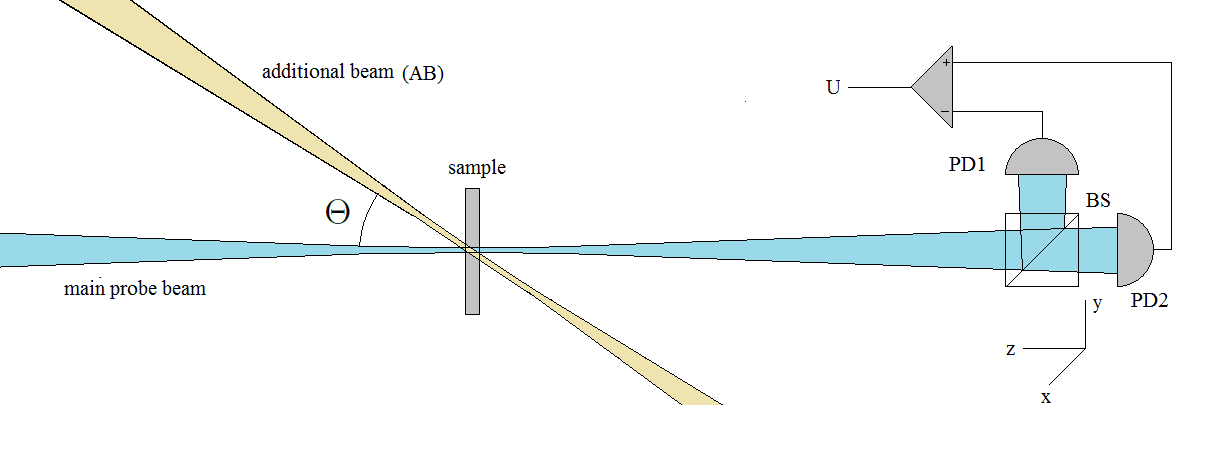
Figure 1: Registration of noise signal produced by additional tilted beam

3 Additional tilted beam

Let us irradiate our sample by an additional beam (AB) tilted by angle $\Theta$ with respect to the main probe beam (Figure (1)). Note that AB do not hit the detector, but scattered field produced by AB can give rise to additional polarimetric signal and our goal now is to calculate it. The calculation can be performed in the same manner as in the previous section with following changes. The scattered field can be calculated by Eq. (8) in which the field ${\bf E_{0}(r)}$ should be replaced by ${\bf E_{0}^{t}(r)}$, where ${\bf E_{0}^{t}(r)}$ represents the field of tilted beam. The field ${\bf E_{0}^{t}(r)}$ can be obtained by rotation of ${\bf E_{0}(r)}$ by angle $\Theta$ around the axis $(\cos\phi,\sin\phi,0)$ parallel to the direction of polarization of the probe beam :

$${\bf E_{0}^{t}(r)}=M{\bf E}_{0}(M{\bf r}).$$ (21)

Here matrix $M$ is defined as

$$M=R(-\phi)H(\Theta)R(\phi)=\left(\matrix{\cos\Theta\sin^{2}\phi+\cos^{2}\phi&[1-\cos\Theta]\sin\phi\cos\phi&-\sin\phi\sin\Theta\cr[1-\cos\Theta]\sin\phi\cos\phi&\cos\Theta\cos^{2}\phi+\sin^{2}\phi&\cos\phi\sin\Theta\cr\sin\Theta\sin\phi&-\sin\Theta\cos\phi&\cos\Theta}\right)=$$ (22)

$$=\left(\matrix{1-{1\over 2}\Theta^{2}\sin^{2}\phi&{1\over 2}\Theta^{2}\sin\phi\cos\phi&-\Theta\sin\phi\cr{1\over 2}\Theta^{2}\sin\phi\cos\phi&1-{1\over 2}\Theta^{2}\cos^{2}\phi&\Theta\cos\phi\cr\Theta\sin\phi&-\Theta\cos\phi&1-{1\over 2}\Theta^{2}}\right)+O(\Theta^{3})$$

Therefore, ${\bf E_{0}^{t}(r)}$ defined by the following expression

$${\bf E_{0}^{t}(r)}=Q\sqrt{2W_{t}\over c}(\cos\phi,\sin\phi,0)\hskip 2.84526pt\exp\imath\bigg{[}kZ({\bf r})-\omega t\bigg{]}\hskip 2.84526pt\exp\bigg{[}-{Q^{2}[X^{2}({\bf r})+Y^{2}({\bf r})]\over 4}\bigg{]}$$ (23)

where

$$\left(\matrix{X({\bf r})\cr Y({\bf r})\cr Z({\bf r})}\right)\equiv\left(\matrix{\cos\Theta\sin^{2}\phi+\cos^{2}\phi&[1-\cos\Theta]\sin\phi\cos\phi&-\sin\phi\sin\Theta\cr[1-\cos\Theta]\sin\phi\cos\phi&\cos\Theta\cos^{2}\phi+\sin^{2}\phi&\cos\phi\sin\Theta\cr\sin\Theta\sin\phi&-\sin\Theta\cos\phi&\cos\Theta}\right)\left(\matrix{x\cr y\cr z}\right)+\left(\matrix{\delta x\cr\delta y\cr\delta z}\right)$$ (24)

with ${\bf r}=(x,y,z)$. We denote by $W_{t}$ the intensity of AB and take into account the possible spatial shift $(\delta x,\delta y,\delta z)$ of AB. Substituting ${\bf E_{0}^{t}(r\textquoteright)}$ (23) to Eq. (8) instead ${\bf E_{0}(r\textquoteright)}$, one can obtain the following expression for scattered field produced by AB:

$$\left(\matrix{{\cal E}_{1x}^{t}\cr{\cal E}_{1y}^{t}}\right)=\left(\matrix{-\sin\phi\cr\cos\phi}\right)\sqrt{2W_{t}\over c}{Qk^{2}\over L}\int\cos(k|{\bf r-r^{\prime}}|)\sin[kZ^{\prime}-\omega t]\exp\bigg{[}-{Q^{2}(X^{\prime 2}+Y^{\prime 2})\over 4}\bigg{]}G_{z}({\bf r^{\prime}})d^{3}{\bf r^{\prime}}$$ (25)

where $X^{\prime}=X({\bf r^{\prime}})$, $Y^{\prime}=Y({\bf r^{\prime}})$ and $Z^{\prime}=Z({\bf r^{\prime}})$, with functions $X({\bf r^{\prime}})$, $Y({\bf r^{\prime}})$, $Z({\bf r^{\prime}})$ defined by Eq. (24), in which $x,y,z\rightarrow x^{\prime},y^{\prime},z^{\prime}$. This formula has the same sense as Eq. (12); for clarity we supply the components of scattered field by $t$. Taking into account this replacements, one can get the relationship for polarimetric signal produced by AB (instead of Eq. (13))

$$u_{1}^{t}=-{4\sqrt{WW_{t}}k^{3}\sin[2\phi]\over cL^{2}}\int_{-l_{x}}^{l_{x}}dx\int_{-l_{y}}^{l_{y}}dy\exp\bigg{[}-{k^{2}(x^{2}+y^{2})\over Q^{2}L^{2}}\bigg{]}\times$$ (26)

$$\times\int\cos(k|{\bf r-r^{\prime}}|)\hskip 2.84526pt\cos\hskip 2.84526ptk\bigg{[}Z^{\prime}-L-{x^{2}+y^{2}\over 2L}\bigg{]}\hskip 2.84526pt\exp\bigg{[}-{Q^{2}(X^{\prime 2}+Y^{\prime 2})\over 4}\bigg{]}G_{z}({\bf r^{\prime}})d^{3}{\bf r^{\prime}}$$

Calculation of intergrals can be carried out in the same manner as it was done in the previous section and the final result for the polarimetric signal produced by AB is:

$$u_{1}^{t}=-{4\sqrt{WW_{t}}k\pi Q^{2}\sin[2\phi]\over c}\int_{V}\cos k[z^{\prime}-Z^{\prime}]\exp\bigg{[}-{Q^{2}(x^{\prime 2}+y^{\prime 2}+X^{\prime 2}+Y^{\prime 2})\over 4}\bigg{]}G_{z}({\bf r^{\prime}})d^{3}{\bf r^{\prime}}$$ (27)

where ${\bf r^{\prime}}=(x^{\prime},y^{\prime},z^{\prime})$

$$\left(\matrix{X^{\prime}\cr Y^{\prime}\cr Z^{\prime}}\right)=\left(\matrix{\cos\Theta\sin^{2}\phi+\cos^{2}\phi&[1-\cos\Theta]\sin\phi\cos\phi&-\sin\phi\sin\Theta\cr[1-\cos\Theta]\sin\phi\cos\phi&\cos\Theta\cos^{2}\phi+\sin^{2}\phi&\cos\phi\sin\Theta\cr\sin\Theta\sin\phi&-\sin\Theta\cos\phi&\cos\Theta}\right)\left(\matrix{x^{\prime}\cr y^{\prime}\cr z^{\prime}}\right)+\left(\matrix{\delta x\cr\delta y\cr\delta z}\right)$$ (28)

Note that $u_{1}^{t}$ is proportional to overlapping between the probe beam and AB and vanish at sufficiently large shift $\delta x,\delta y,\delta z$. Trigonometric factor $\cos k[z\textquoteright-Z\textquoteright]$ is, in fact, emphasize the harmonic of gyrotropy with spatial frequency equal to difference between the wave vectors of probe beam and AB. Total signal in presence of both probe and AB is the sum of (19) and (27): $u_{1}+u_{1}^{t}$. Remind that angle $\Theta$ should be not too large. In the opposite case one should take into account the component ${\bf E_{1}^{2}(r)}$ in Eq. (8).

4 Noise signal produced by probe and additional beams simultaneously

Noise signal produced by probe beam and AB is calculated as Fourier transform of the total polarimetric signal $u=u_{1}+u^{t}_{1}$ correlation function. It consists of 3 terms:

$${\cal N}_{t}(\nu)=\int dte^{\imath\nu t}\langle u(0)u(t)\rangle=\int dte^{\imath\nu t}\bigg{[}\langle u_{1}(0)u_{1}(t)\rangle+2\langle u_{1}(0)u_{1}^{t}(t)\rangle+\langle u_{1}^{t}(0)u_{1}^{t}(t)\rangle\bigg{]}$$ (29)

Using Eq’s (19) and (27) one can write the expressions for each of these terms. The first term has been already calculated and is difined by Eq. (20). For correlator entering the last term we have the following expression

$$\langle u_{1}^{t}(0)u_{1}^{t}(t)\rangle={16WW_{t}k^{2}\pi^{2}Q^{4}\sin^{2}[2\phi]\over c^{2}}\int_{V}d^{3}{\bf r}\int_{V}d^{3}{\bf r^{\prime}}\cos k[z-Z]\cos k[z^{\prime}-Z^{\prime}]\times$$ (30)

$$\times\exp\bigg{[}-{Q^{2}(X^{2}+Y^{2}+x^{2}+y^{2}+X^{\prime 2}+Y^{\prime 2}+x^{\prime 2}+y^{\prime 2})\over 4}\bigg{]}\times\langle G_{z}({\bf r^{\prime}},0)G_{z}({\bf r},t)\rangle,$$

where $x,y,z\rightarrow{\bf r}$ and $X,Y,Z$ are defined by relationship Eq. (28)

$$\left(\matrix{X\cr Y\cr Z}\right)=\left(\matrix{\cos\Theta\sin^{2}\phi+\cos^{2}\phi&[1-\cos\Theta]\sin\phi\cos\phi&-\sin\phi\sin\Theta\cr[1-\cos\Theta]\sin\phi\cos\phi&\cos\Theta\cos^{2}\phi+\sin^{2}\phi&\cos\phi\sin\Theta\cr\sin\Theta\sin\phi&-\sin\Theta\cos\phi&\cos\Theta}\right)\left(\matrix{x\cr y\cr z}\right)+\left(\matrix{\delta x\cr\delta y\cr\delta z}\right)$$ (31)

$X^{\prime},Y^{\prime},Z^{\prime}$ are similar functions of $x^{\prime},y^{\prime},z^{\prime}\rightarrow{\bf r^{\prime}}$.

Finally, the cross correlator $\langle u_{1}^{t}(0)u_{1}(t)\rangle$ can be written as

$$\langle u_{1}^{t}(0)u_{1}(t)\rangle={16W\sqrt{WW_{t}}k^{2}\pi^{2}Q^{4}\sin^{2}[2\phi]\over c^{2}}\int_{V}d^{3}{\bf r}\int_{V}d^{3}{\bf r^{\prime}}\cos k[z-Z]\times$$ (32)

$$\times\exp\bigg{[}-{Q^{2}(X^{2}+Y^{2}+x^{2}+y^{2})\over 4}-{Q^{2}(x^{\prime 2}+y^{\prime 2})\over 2}\bigg{]}\times\langle G_{z}({\bf r^{\prime}},0)G_{z}({\bf r},t)\rangle$$

Let us now consider the sence of various factors entering Eqs.(20,30,32).

Exponential factor reduce the region of integration to the region of overlapping of the probe beam and AB. If $\Theta$ is not too large and $l_{s}\Theta<w$, this region is close to “beam volume within the sample”. In this case exponential factor can be calculated at $X=x,Y=y,Z=z,X^{\prime}=x^{\prime},Y^{\prime}=y^{\prime},Z^{\prime}=z^{\prime}$. Note that it is rather difficult to satisfy the condition $l_{s}\Theta<w$ in real experiment. For this reason overlapping factor may considerably reduce the contribution of AB to polarimetric signal.

Trigonometric factor at small angles $\Theta$ depends on difference between wave vectors of probe beam and AB because cosine argument can be evaluated as $z-Z=[\cos\phi y-\sin\phi x]\Theta$.

Correlation function $\langle G_{z}({\bf r^{\prime}},0)G_{z}({\bf r},t)\rangle$ defined by a concrete model of gyrotropic medium. For homogeneous mediums it depends on the difference ${\bf r-r^{\prime}}$ of space arguments. For the model of independent paramagnetic centers described below $\langle G_{z}({\bf r^{\prime}},0)G_{z}({\bf r},t)\rangle$ $\sim\delta({\bf r-r^{\prime}})e^{-|t|/\tau}\cos\omega_{0}t$

If concrete model of gyrotropic medium is specified, then the integrals entering Eqs.(20,30,32) can be calculated in the frame of this model. In the next section we will present calculation for the model of independent paramagnetic centers. Nevertheless, the following general remarks can be made. Suppose that beam waste $4w$ and sample length $l_{s}$ are much greater than correlation radius of gyrotropy $R_{c}$ and spatial period $2\pi/k\Theta$ related to the difference of wave vectors of the probe beam and AB: $4w,l_{s}\gg R_{c},2\pi/k\Theta$. Then, one can replace variables in integrals entering Eqs.(20,30,32) in the following way: ${\bf r,r^{\prime}}\rightarrow{\bf R\equiv r-r^{\prime},R^{\prime}\equiv r+r^{\prime}}$ and take advantage of the fact that correlator $\langle G_{z}({\bf r^{\prime}},0)G_{z}({\bf r},t)\rangle$ depends on difference of its arguments:

$$\langle G_{z}({\bf r^{\prime}},0)G_{z}({\bf r},t)\rangle\equiv K({\bf r-r^{\prime}},t)$$ (33)

Then, the integral over ${\bf R\equiv r-r^{\prime}}$ in Eq. (20) can be estimated as the average of $K({\bf R},t)$ over irradiated volume of the sample $V_{b}$. The integration over ${\bf R^{\prime}\equiv r+r^{\prime}}$ gives this volume itself and we obtain

$${\cal N}(\nu)={16W^{2}k^{2}\pi^{2}Q^{4}\sin^{2}[2\phi]\over c^{2}}\int dt\hskip 2.84526pte^{\imath\nu t}\int_{V}d{\bf r}d{\bf r^{\prime}}\exp\bigg{[}-{Q^{2}(x^{\prime 2}+y^{\prime 2}+x^{2}+y^{2})\over 2}\bigg{]}K({\bf r-r^{\prime}},t)\sim$$ (34)

$$\sim{W^{2}l_{s}\sin^{2}[2\phi]\over S}\int dt\hskip 2.84526pte^{\imath\nu t}\int_{V_{b}}d{\bf R}\hskip 2.84526ptK({\bf R},t).$$

Here we denote the cross section area of the beam by $S\equiv 4\pi w^{2}$ and take into account that $w=1/Q$ and that irradiated volume of the sample is $V_{b}=Sl_{s}$, where $l_{s}$ is the sample length.

The correlation function Eq.(30) can be estimated in a similar way. If $\Theta$ is not too large the arguments of cosine functions can be evaluated as: $z-Z=[\cos\phi y-\sin\phi x]\Theta$ and $z^{\prime}-Z^{\prime}=[\cos\phi y^{\prime}-\sin\phi x^{\prime}]\Theta$. Therefore, one can represent the product of cosine functions in Eq.(30) as

$$\cos k[z-Z]\cos k[z^{\prime}-Z^{\prime}]={1\over 2}\cos\bigg{\{}k\Theta\bigg{[}(y-y^{\prime})\cos\phi-(x-x^{\prime})\sin\phi\bigg{]}\bigg{\}}+$$

$$+{1\over 2}\cos\bigg{\{}k\Theta\bigg{[}(y+y^{\prime})\cos\phi-(x+x^{\prime})\sin\phi\bigg{]}\bigg{\}}$$

Note that difference $\Delta{\bf k}$ between the wave vector of the probe beam and AB for small $\Theta$ has only $x$ and $y$ components: $\Delta{\bf k}=k\Theta(-\sin\phi,\cos\phi,0)$. Therefore, this relationship after replacement of variables ${\bf r,r^{\prime}}\rightarrow{\bf R=r-r^{\prime},R^{\prime}=r+r^{\prime}}$ takes the form

$$\cos k[z-Z]\cos k[z^{\prime}-Z^{\prime}]={1\over 2}\cos(\Delta{\bf k,R})+{1\over 2}\cos(\Delta{\bf k,R^{\prime}})$$

Remind that our treatment is valid if $w$ is large enough for $\Delta kw>2\pi$. In this case the integral $\int_{V_{b}}d{\bf R^{\prime}}\cos(\Delta{\bf k,R^{\prime}})\sim 0$ and we come to the conclusion that correlation function Eq. (30) can be estimated as follows

$$\langle u_{1}^{t}(0)u_{1}^{t}(t)\rangle\sim{WW_{t}Q^{4}\sin^{2}[2\phi]}\int_{V_{b}}d{\bf R}d{\bf R^{\prime}}\hskip 2.84526ptK({\bf R},t)\cos(\Delta{\bf k,R})\sim$$ (35)

$$\sim{WW_{t}\sin^{2}[2\phi]l_{s}\over S}\int_{V_{b}}d{\bf R}\hskip 2.84526ptK({\bf R},t)\cos(\Delta{\bf k,R})$$

Therefore, the contribution of tilted AB to noise signal is proportional to the Fourier transform of correlation function of gyrotropy calculated at differential wave vector of the probe and additional beams $\Delta{\bf k}$. Analogously it can be shown that contribution of cross correlator Eq. (32) is relatively small under considered conditions.

5 Model of independent paramagnetic centers

It this model the random field of gyrotropy $G_{z}({\bf r})$ has the form

$$G_{z}({\bf r})=\sum_{i=1}^{N}g_{i}(t)\delta({\bf r-r_{i}}),$$ (36)

corresponding to $N$ paramagnetic centers randomly distributed in space with some density $\sigma$ defined as $\sigma\equiv N/V$ where $V$ is total volume of the system. We accept that $g_{i}(t)$ is proportional to $z$-component of magnetization of $i$-th center. The polarimetric signal can be calculated by Eq.(19):

$$u_{1}=u_{1}(t)=-{4Wk\pi Q^{2}\sin[2\phi]\over c}\int_{V}\exp\bigg{[}-{Q^{2}(x^{\prime 2}+y^{\prime 2})\over 2}\bigg{]}\sum_{i}g_{i}(t)\delta({\bf r^{\prime}-r_{i}})d^{3}{\bf r^{\prime}}$$ (37)

Let us calculate polarimetric signal $u_{10}$ produced by a sample in which all magnetizations $g_{i}(t)$ are constant and equal to each other: $g_{i}(t)=g_{0}=$ const. This corresponds to paramagnet placed in a high magnetic field at low temperatures. Formula Eq. (37) gives

$$u_{10}=-{8Wkg_{0}\sigma l_{s}\pi^{2}\sin[2\phi]\over c}$$ (38)

We will see below that $u_{10}$ is a convenient scale. Let us now consider the state of our gyrotropic medium for which the quantities $g_{i}$ are not constants but represent stationary random processes with following correlation function: $\langle g_{i}(t)g_{k}(t^{\prime})\rangle=\delta_{ik}K(t-t\textquoteright)$ (do not confuse with space-time correlation function Eq. (33)) and calculate the noise power spectrum Eq. (20) for this model. We have

$$\langle G_{z}({\bf r^{\prime}},0)G_{z}({\bf r},t)\rangle={1\over V}\sum_{i}\int d^{3}{\bf r_{i}}\langle g_{i}(0)g_{i}(t)\rangle\delta({\bf r^{\prime}-r_{i}})\delta({\bf r-r_{i}})=\delta({\bf r-r^{\prime}})\sigma K(t),$$ (39)

and, consequently

$${\cal N}(\nu)={16W^{2}k^{2}\pi^{3}Q^{2}l_{s}\sigma\sin^{2}[2\phi]\over c^{2}}\int dt\hskip 2.84526pte^{\imath\nu t}K(t)$$ (40)

If we accept for beam area the expression $S=4\pi w^{2}$, then $Q^{2}=1/w^{2}=4\pi/S$. Taking into account Eq. (38) we obtain the following relationship for noise power spectrum

$${\cal N}(\nu)={u_{10}^{2}\over\sigma l_{s}S}\hskip 2.84526pt\int dte^{\imath\nu t}{\langle g(0)g(t)\rangle\over g_{0}^{2}}$$ (41)

Note that $\sigma l_{s}S\equiv N_{b}$ is the number of centers in the irradiated volume of the sample.

In the simplest case each paramagnetic center of our gyrotropic medium can be associated with effective spin 1/2 . In this case the total magnetization can be expressed as: $g_{0}^{2}=(g\beta)^{2}/4$ (here $g$ is effective $g$-factor and $\beta$ is Bohr magneton). If the transverse magnetic field $B_{x}$ is applied the correlator $\langle g(0)g(t)\rangle$ can be calculated by following chain of relationships:

$$\langle g(0)g(t)\rangle={(g\beta)^{2}\over 2}\hbox{ Sp }[S_{z}S_{z}(t)+S_{z}(t)S_{z}]\rho_{eq}\hskip 28.45274ptS_{z}(t)=e^{-\imath\omega_{0}tS_{x}}S_{z}e^{\imath\omega_{0}tS_{x}}\hskip 14.22636pt\omega_{0}\equiv{g\beta B_{x}\over\hbar}$$ (42)

Here $\rho_{eq}$ is the density matrix of two-level system representing our effective spin 1/2. If temperature is high enough for $kT\gg g\beta B_{x}$, the density matrix can be taken constant $\rho_{eq}=\hat{I}/2$ ($\hat{I}$ is the unit matrix) and we obtain

$$\langle g(0)g(t)\rangle={(g\beta)^{2}\over 4}\hbox{ Sp }[S_{z}S_{z}(t)+S_{z}(t)S_{z}]={(g\beta)^{2}\over 4}\hskip 2.84526pt\cos\omega_{0}t\rightarrow{(g\beta)^{2}\over 4}\hskip 2.84526pte^{-|t|/\tau}\cos\omega_{0}t\hskip 14.22636pt\Rightarrow$$ (43)

$$\Rightarrow{\langle g(0)g(t)\rangle\over g_{0}^{2}}=e^{-|t|/\tau}\cos\omega_{0}t$$

We introduce phenomenologically the transverse relaxation time $\tau$. For noise power spectrum we get

$${\cal N}(\nu)={u_{10}^{2}\tau\over N_{b}}\hskip 2.84526pt\bigg{[}{1\over 1+(\omega_{0}+\nu)^{2}\tau^{2}}+{1\over 1+(\omega_{0}-\nu)^{2}\tau^{2}}\bigg{]}$$ (44)

The root-mean-square of polarimetric noise is defined by following relationship

$$\langle\delta u^{2}\rangle={1\over 2\pi}\int{\cal N}(\nu)d\nu={u_{10}^{2}\over N_{b}}$$ (45)

In the similar way one can calculate the power spectrum of polarimetric noise Eqs. (20,30,32) in presence of AB. Using the relationship Eq. (38) for correlation function and Eqs. (20,30,32), one can obtain:

$$\langle u(0)u(t)\rangle=u_{10}^{2}{e^{-|t|/\tau}\cos\omega_{0}t\over N_{b}}\bigg{[}1+2\sqrt{W_{t}\over W}\exp\bigg{[}-{k^{2}\Theta^{2}\over 4Q^{2}}\bigg{]}+{W_{t}\over W}{1\over 2}\bigg{(}1+\exp\bigg{[}-{k^{2}\Theta^{2}\over Q^{2}}\bigg{]}\bigg{)}\bigg{]}$$ (46)

If $2\pi/k=1\mu$m, $\Theta\sim 0.1$ and $1/Q\sim 30\mu$m, the exponential factors can be omitted and simplified expressions for correlation function and noise power spectrum take the form

$$\langle u(0)u(t)\rangle={u_{10}^{2}\over N_{b}}\bigg{[}1+{W_{t}\over 2W}\bigg{]}e^{-|t|/\tau}\cos\omega_{0}t$$ (47)

$${\cal N}(\nu)={u_{10}^{2}\tau\over N_{b}}\hskip 2.84526pt\bigg{[}1+{W_{t}\over 2W}\bigg{]}\bigg{[}{1\over 1+(\omega_{0}+\nu)^{2}\tau^{2}}+{1\over 1+(\omega_{0}-\nu)^{2}\tau^{2}}\bigg{]}$$ (48)

It is seen from Eq. (48) that if $W_{t}\sim W$, switching of additional beam leads to 50$\%$ increasing of the noise power and seems can be easily observed. Note once again that we suppose complete overlapping of the probe and AB which may be not the case. For this reason the contribution of AB to noise power spectrum in real experiment may be less than predicted by Eqs. (47, 48).

Conclusion

We develop a single scattering theory for the purposes of optical spin noise spectroscopy. For introduced model of polarimetric detector we calculate its output signal produced by Gaussian beam probing the sample with specified gyrotropy and show that this signal is proportional to the sample’s gyrotropy averaged over irradiated volume. We calculate the signal produced by additional probe beam tilted with respect to the main one and show that this signal is proportional to the Fourier transformation of gyrotropy calculated for the differential wave vector of the main and additional beam. The noise signals within the model of independent paramagnetic centers are also calculated.

References

• [1] E.B.Aleksandrov and V.S.Zapasskii, “Magnetic resonance in the Faraday rotation noise spectrum”, JETP, 54, 64 (1981)
• [2] V. S. Zapasskii, Adv. Opt. Photon., 5, 131 (2013)
• [3] G.M.Muller, M.Oestreich, M.Romer, and J.Hubner, “Semiconductor spin noise spectroscopy: Fundamentals, accomplishments, and challenges” Physics E, 43, 569 (2010)
• [4] N A Sinitsyn1 and Yu V Pershin, Rep. Prog. Phys. 79 106501 (2016)
• [5] M. Oestreich, M. Roemer, R. G. Haug, and D. Hagele, Phys. Rev. Lett., 95, 216603 (2005)
• [6] I. I. Ryzhov, S. V. Poltavtsev, K. V. Kavokin, M. M. Glazov, G. G. Kozlov, M. Vladimirova, D. Scalbert, S. Cronenberger, A. V. Kavokin, A. Lema?tre, J. Bloch, and V. S. Zapasskii, Measurements of nuclear spin dynamics by spin-noise spectroscopy, Appl. Phys. Lett. 106, 242405 (2015).
• [7] Ivan I. Ryzhov, Gleb G. Kozlov, Dmitrii S. Smirnov, Mikhail M. Glazov, Yurii P. Efimov, Sergei A. Eliseev, Viacheslav A. Lovtcius, Vladimir V. Petrov, Kirill V. Kavokin, Alexey V. Kavokin, and Valerii S. Zapasski, Spin noise explores local magnetic fields in a semiconductor, Sci. Rep. 6, 21062 (2016) [see also Supplementary information].
• [8] V. S. Zapasskii, A. Greilich, S. A. Crooker, Yan Li, G. G. Kozlov, D. R. Yakovlev, D. Reuter, A. D. Wieck, and M. Bayer, “Optical spectroscopy of spin noise,” Phys. Rev. Lett., vol. 110, 176601 (2013)
• [9] B.M. Gorbovitskii and V.I. Perel, Opt. Spektrosk. 54, 388-390 (1983)
• [10] S. Cronenberger and D. Scalbert, REVIEW OF SCIENTIFIC INSTRUMENTS 87, 093111 (2016)