Efficient spectral computation of the stationary states of rotating Bose-Einstein condensates by the preconditioned nonlinear conjugate gradient method

Abstract

We propose a preconditioned nonlinear conjugate gradient method coupled with a spectral spatial discretization scheme for computing the ground states (GS) of rotating Bose-Einstein condensates (BEC), modeled by the Gross-Pitaevskii Equation (GPE). We first start by reviewing the classical gradient flow (also known as imaginary time (IMT)) method which considers the problem from the PDE standpoint, leading to numerically solve a dissipative equation. Based on this IMT equation, we analyze the forward Euler (FE), Crank-Nicolson (CN) and the classical backward Euler (BE) schemes for linear problems and recognize classical power iterations, allowing us to derive convergence rates. By considering the alternative point of view of minimization problems, we propose the preconditioned gradient (PG) and conjugate gradient (PCG) methods for the GS computation of the GPE. We investigate the choice of the preconditioner, which plays a key role in the acceleration of the convergence process. The performance of the new algorithms is tested in 1D, 2D and 3D. We conclude that the PCG method outperforms all the previous methods, most particularly for 2D and 3D fast rotating BECs, while being simple to implement.

1 Introduction

Bose-Einstein Condensates (BECs) were first predicted theoretically by S.N. Bose and A. Einstein, before being realized experimentally in 1995 [4, 20, 27, 30]. This state of matter has the interesting feature that macroscopic quantum physics properties can emerge and be observed in laboratory experiments. The literature on BECs has grown extremely fast over the last 20 years in atomic, molecular, optics and condensed matter physics, and applications from this new physics are starting to appear in quantum computation for instance [22]. Among the most important directions, a particular attention has been paid towards the understanding of the nucleation of vortices [1, 21, 34, 35, 36, 38, 45] and the properties of dipolar gases [13, 14] or multi-components BECs [11, 12, 13]. At temperatures $T$ which are much smaller than the critical temperature $T_{c}$, the macroscopic behavior of a BEC can be well described by a condensate wave function $\psi$ which is solution to a Gross-Pitaevskii Equation (GPE). Being able to compute efficiently the numerical solution of such a class of equations is therefore extremely useful. Among the most crucial questions are the calculations of stationary states, i.e. ground/excited states, and of the real-time dynamics [5, 9, 13].

To fully analyze a representative and nontrivial example that can be extended to other more general cases, we consider in this paper a BEC that can be modeled by the rotating (dimensionless) GPE. In this setting, the computation of a ground state of a $d$-dimensional BEC takes the form of a constrained minimization problem: find $\phi\in L^{2}(\mathbb{R}^{d})$ such that

$$\phi\in\operatorname*{arg\,min}_{\left\|\phi\right\|=1}E(\phi),$$

where $E$ is the associated energy functional. Several approaches can be developed for computing the stationary state solution to the rotating GPE. For example, some techniques are based on appropriate discretizations of the continuous normalized gradient flow/imaginary-time formulation [3, 7, 9, 13, 15, 19, 25, 26, 46], leading to various iterative algorithms. These approaches are general and can be applied to many situations (dipolar interactions, multi-components GPEs…). We refer for instance to the recent freely distributed Matlab solver GPELab that provides the stationary states computation [6] (and real-time dynamics [8]) for a wide variety of GPEs based on the so-called BESP (Backward Euler pseudoSPectral) scheme [7, 9, 13, 15] (see also Sections 4 and 6). Other methods are related to the numerical solution of the nonlinear eigenvalue problem [31, 43] or on optimization techniques under constraints [17, 23, 28, 29]. As we will see below in Section 4, some connections exist between these approaches. Finally, a regularized Newton-type method was proposed recently in [44].

Optimization problems with orthogonal or normalization constraints also occur in different branches of computational science. An elementary but fundamental example is the case of a quadratic energy, where solving the minimization problem is equivalent to finding an eigenvector associated with the lowest eigenvalue of the symmetric matrix representing the quadratic form. A natural generalization is a class of orthogonalized minimization problems, which for a quadratic energy reduce to finding the $N$ first eigenvectors of a matrix. Many problems in electronic structure theory are of this form, including the celebrated Kohn-Sham and Hartree-Fock models [24, 41]. Correspondingly, a large amount of effort has been devoted to finding efficient discretization and minimization schemes. A workhorse of these approaches is the nonlinear preconditioned conjugate gradient method, developed in the 80s [37], as well as several variants of this (the Davidson algorithm, or the LOBPCG method [33]).

Although similar, there are significant differences between the mathematical structure of the problem in electronic structure theory and the Gross-Pitaevskii equation. In some respects, solving the GPE is easier: there is only one wavefunction (or only a few for multi-species gases), and the nonlinearity is often local (at least when dipolar effects are not taken into account), with a simpler mathematical form than many electronic structure models. On the other hand, the Gross-Pitaevskii equation describes the formation of vortices: the discretization schemes must represent these very accurately, and the energy landscape presents shallower minima, leading to a more difficult optimization problem.

In the present paper, we consider the constrained nonlinear conjugate gradient method for solving the rotating GPE (Section 2) with a pseudospectral discretization scheme (see Section 3). This approach provides an efficient and robust way to solve the minimization problem. Before introducing the algorithm, we review in Section 4 the discretization of the gradient flow/imaginary-time equation by standard schemes (explicit/implicit Euler and Crank-Nicolson schemes). This enables us to make some interesting and meaningful connections between these approaches and some techniques related to eigenvalue problems, such as the power method. In sections 5.1 and 5.2, we introduce the projected preconditioned gradient (PG) and preconditioned conjugate gradient (PCG) methods for solving the minimization problem on the Riemannian manifold defined by the spherical constraints. In particular, we provide some formulae to compute the stepsize arising in such iterative methods to get the energy decay assumption fulfilled. The stopping criteria and convergence analysis are discussed in sections 5.3 and 5.4. We then investigate the design of preconditioners (section 5.5). In particular, we propose a new simple symmetrical combined preconditioner, denoted by $P_{\textrm{C}}$. In Section 6, we consider the numerical study of the minimization algorithms for the 1D, 2D and 3D GPEs (without and with rotation). We first propose in section 6.1 a thorough analysis in the one-dimensional case. This shows that the PCG approach with combined preconditioner $P_{\textrm{C}}$ and pseudospectral discretization, called PCG${}_{\textrm{C}}$ method, outperforms all the other approaches, most particularly for very large nonlinearities. In sections 6.2 and 6.3, we confirm these properties in 2D and 3D, respectively, and show how the PCG_C algorithm behaves with respect to increasing the rotation speed. Finally, section 7 provides a conclusion.

2 Definitions and notations

The problem we consider is the following: find $\phi\in L^{2}(\mathbb{R}^{d})$ such that

$$\phi\in\operatorname*{arg\,min}_{\left\|\phi\right\|=1}E(\phi).$$ (2.1)

We write $\displaystyle\left\|\phi\right\|=\int_{\mathbb{R}^{d}}|\phi|^{2}$ for the standard $L^{2}$-norm and the energy functional $E$ is defined by

$$E(\phi) =\int_{\mathbb{R}^{d}}\left[\frac{1}{2}|\nabla\phi|^{2}+V(\mathbf{x})|\phi|^{2}+\frac{\eta}{2}|\phi|^{4}-\omega\phi^{*}L_{z}\phi\right],$$

where $V$ is an external potential, $\eta$ is the nonlinearity strength, $\omega$ is the rotation speed, and $L_{z}=i(y\partial_{x}-x\partial_{y})$ is the angular momentum operator.

A direct computation of the gradient of the energy leads to

$$\nabla E(\phi) =2H_{\phi}\phi,\quad\text{with}\quad H_{\phi}=-\frac{1}{2}\Delta+V+\eta|\phi|^{2}-\omega L_{z}$$

the mean-field Hamiltonian. We can compute the second-order derivative as

$$\displaystyle\frac{1}{2}\nabla^{2}E(\phi)[f,f]=\left\langle f,H_{\phi}f\right\rangle+\eta\operatorname{Re}\left\langle\phi^{2},f^{2}\right\rangle.$$

We introduce $\mathcal{S}=\{\phi\in L^{2}(\mathbb{R}^{d}),\left\|\phi\right\|=1\}$ as the spherical manifold associated to the normalization constraint. Its tangent space at a point $\phi\in\mathcal{S}$ is $T_{\phi}\mathcal{S}=\{h\in L^{2}(\mathbb{R}^{d}),\operatorname{Re}\left\langle\phi,h\right\rangle=0\}$, and the orthogonal projection $M_{\phi}$ onto this space is given by $M_{\phi}h=h-\operatorname{Re}\left\langle\phi,h\right\rangle\phi$.

The Euler-Lagrange equation (first-order necessary condition) associated with the problem (2.1) states that, at a minimum $\phi\in\mathcal{S}$, the projection of the gradient on the tangent space is zero, which is equivalent to

$$H_{\phi}\phi=\lambda\phi,$$

where $\lambda=\left\langle H_{\phi}\phi,\phi\right\rangle$ is the Lagrange multiplier associated to the spherical constraint, and is also known as the chemical potential. Therefore, the minimization problem can be seen as a nonlinear eigenvalue problem. The second-order necessary condition states that, for all $h\in T_{\phi}\mathcal{S}$,

$$\frac{1}{2}\nabla^{2}E(\phi)[h,h]-\lambda\left\|h\right\|^{2}\geq 0.$$

For a linear problem ($\eta=0$) and for problems where the nonlinearity has a special structure (for instance, the Hartree-Fock model), this implies that $\lambda$ is the lowest eigenvalue of $H_{\phi}$ (a property known as the Aufbau principle in electronic structure theory). This property is not satisfied here.

3 Discretization

To find a numerical solution of the minimization problem, the function $\phi\in L^{2}(\mathbb{R}^{d})$ must be discretized. The presence of vortices in the solution imposes strong constraints on the discretization, which must be accurate enough to resolve fine details. Several discretization schemes have been used to compute the solution to the GPE, including high-order finite difference schemes or finite element schemes with adaptive meshing strategies [28, 29]. Here, we consider a standard pseudo-spectral discretization based on Fast Fourier Transforms (FFTs) [7, 9, 15, 46].

We truncate the wave function $\phi$ to a square domain $[-L,L]^{d}$, with periodic boundary conditions, and discretize $\phi$ with the same even number of grid points $M$ in any dimension. These two conditions can of course be relaxed to a different domain size $L$ and number of points $M$ in each dimension, at the price of more complex notations. We describe our scheme in 2D, its extension to other dimensions being straightforward. We introduce a uniformly sampled grid: $\mathcal{D}_{M}\mathrel{\mathop{\mathchar 58\relax}}=\{\mathbf{x}_{k_{1},k_{2}}=(x_{k_{1}},y_{k_{2}})\}_{(k_{1},k_{2})\in\mathcal{O}_{M}}$, with $\mathcal{O}_{M}\mathrel{\mathop{\mathchar 58\relax}}=\{0,\ldots,M-1\}^{2}$, $x_{k_{1}+1}-x_{k_{1}}=y_{k_{2}+1}-y_{{k}_{2}}=h$, with mesh size $h=2L/M$, $M$ an even number. We define the discrete Fourier frequencies $(\xi_{p},\mu_{q})$, with $\xi_{p}=p{\pi}/{L},-M/2\leq p\leq M/2-1$, and $\mu_{q}=q{\pi}/{L},-M/2\leq q\leq M/2-1$. The pseudo-spectral approximations $\widetilde{\phi}$ of the function $\phi$ in the $x$- and $y$-directions are such that

$$\begin{array}[]{l}\displaystyle\widetilde{\phi}(t,x,y)=\frac{1}{M}\sum_{p=-M/2}^{M/2-1}\widehat{\widetilde{\phi}_{p}}(t,y)e^{i\xi_{p}(x+L)},\hskip 56.9055pt\displaystyle\widetilde{\phi}(t,x,y)=\frac{1}{M}\sum_{q=-M/2}^{M/2-1}\widehat{\widetilde{\phi}_{q}}(t,x)e^{i\mu_{q}(y+L)},\end{array}$$

where $\widehat{\widetilde{\phi}_{p}}$ and $\widehat{\widetilde{\phi}_{q}}$ are respectively the Fourier coefficients in the $x$- and $y$-directions

$$\begin{array}[]{l}\displaystyle\widehat{\widetilde{\phi}_{p}}(t,y)=\sum_{k_{1}=0}^{M-1}\widetilde{\phi}_{k_{1}}(t,y)e^{-i\xi_{p}(x_{k_{1}}+L)},\hskip 56.9055pt\displaystyle\widehat{\widetilde{\phi}_{q}}(t,x)=\sum_{k_{2}=0}^{M-1}\widetilde{\phi}_{k_{2}}(t,x)e^{-i\mu_{q}(y_{k_{2}}+L)}.\end{array}$$

The following notations are used: $\widetilde{\phi}_{k_{1}}(t,y)=\widetilde{\phi}(t,x_{k_{1}},y)$ and $\widetilde{\phi}_{k_{2}}(t,x)=\widetilde{\phi}(t,x,y_{k_{2}})$. In order to evaluate the operators, we introduce the matrices

$$\mathbb{I}_{k_{1},k_{2}}\mathrel{\mathop{\mathchar 58\relax}}=\delta_{k_{1},k_{2}},\hskip 28.45274pt[[V]]_{k_{1},k_{2}}\mathrel{\mathop{\mathchar 58\relax}}=V(\mathbf{x}_{k_{1},k_{2}}),\hskip 28.45274pt[[|\phi|^{2}]]_{k_{1},k_{2}}=|\phi_{k_{1},k_{2}}|^{2},$$

for $(k_{1},k_{2})\in\mathcal{O}_{M}$, and $\delta_{k_{1},k_{2}}$ being the Dirac delta symbol which is equal to $1$ if and only if $k_{1}=k_{2}$ and $0$ otherwise. We also need the operators $[[\partial^{2}_{x}]]$, $[[\partial^{2}_{y}]]$, $y[[\partial_{x}]]$ and $x[[\partial_{y}]]$ which are applied to the approximation $\widetilde{\phi}$ of $\phi$, for $(k_{1},k_{2})\in\mathcal{O}_{M}$,

$$\begin{array}[]{l}\displaystyle\partial^{2}_{x}\phi(\mathbf{x}_{k_{1},k_{2}})\approx([[\partial^{2}_{x}]]\widetilde{\phi})_{k_{1},k_{2}}\mathrel{\mathop{\mathchar 58\relax}}=-\frac{1}{M}\sum_{p=-M/2}^{M/2-1}\xi^{2}_{p}\widehat{(\widetilde{\phi}_{k_{2}})}_{p}e^{i\xi_{p}(x_{k_{1}}+L)},\\[14.22636pt] \displaystyle\partial^{2}_{y}\phi(\mathbf{x}_{k_{1},k_{2}})\approx([[\partial^{2}_{y}]]\widetilde{\phi})_{k_{1},k_{2}}\mathrel{\mathop{\mathchar 58\relax}}=-\frac{1}{M}\sum_{q=-M/2}^{M/2-1}\mu^{2}_{q}\widehat{(\widetilde{\phi}_{k_{1}})}_{q}e^{i\mu_{q}(y_{k_{2}}+L)},\\[14.22636pt] \displaystyle(x\partial_{y}\phi)(\mathbf{x}_{k_{1},k_{2}})\approx(x[[\partial_{y}]]\widetilde{\phi})_{k_{1},k_{2}}\mathrel{\mathop{\mathchar 58\relax}}=\frac{1}{M}\sum_{q=-M/2}^{M/2-1}ix_{k_{1}}\mu_{q}\widehat{(\widetilde{\phi}_{k_{1}})}_{q}e^{i\mu_{q}(y_{k_{2}}+L)},\\[14.22636pt] \displaystyle(y\partial_{x}\phi)(\mathbf{x}_{k_{1},k_{2}})\approx(y[[\partial_{x}]]\widetilde{\phi})_{k_{1},k_{2}}\mathrel{\mathop{\mathchar 58\relax}}=\frac{1}{M}\sum_{p=-M/2}^{M/2-1}iy_{k_{2}}\xi_{p}\widehat{(\widetilde{\phi}_{k_{2}})}_{p}e^{i\xi_{p}(x_{k_{1}}+L)}.\end{array}$$ (3.2)

By considering the operators from $\mathbb{C}^{N}$ ($N=M^{2}$ (in 2D)) to $\mathbb{C}$ given by $[[\Delta]]\mathrel{\mathop{\mathchar 58\relax}}=[[\partial^{2}_{x}]]+[[\partial^{2}_{y}]]$ and $[[\mathbb{L}_{z}]]\mathrel{\mathop{\mathchar 58\relax}}=-i(x[[\partial_{y}]]-y[[\partial_{x}]])$, we obtain the discretization of the gradient of the energy

$$\nabla E(\phi)=2H_{\phi}\phi,\quad\textrm{ with }H_{\phi}=-\frac{1}{2}[[\Delta]]+[[V]]+\eta[[|\phi|^{2}]]-\omega[[L_{z}]].$$

We set $\phi\mathrel{\mathop{\mathchar 58\relax}}=(\tilde{\phi}(\mathbf{x}_{k_{1},k_{2}}))_{(k_{1},k_{2})\in\mathcal{O}_{M}}$ as the discrete unknown vector in $\mathbb{C}^{N}$. For conciseness, we identify an array $\phi$ in the vector space of 2D complex-valued arrays $\mathcal{M}_{M}(\mathbb{C})$ (storage according to the 2D grid) and the reshaped vector in $\mathbb{C}^{N}$. Finally, the cost for evaluating the application of a 2D FFT is $\mathcal{O}(N\log N)$.

In this discretization, the computations of Section 2 are still valid, with the following differences: $\phi$ is an element of $\mathbb{C}^{N}$, the operators $\Delta$, $V$, $|\phi|^{2}$ and $L_{z}$ are $N\times N$ hermitian matrices, and the inner product is the standard $\mathbb{C}^{N}$ inner product. In the following sections, we will assume a discretization like the above one, and drop the brackets in the operators for conciseness.

4 Review and analysis of classical methods for computing the ground states of GPEs

Once an appropriate discretization is chosen, it remains to compute the solution to the discrete minimization problem

$$\phi\in\operatorname*{arg\,min}_{\phi\in\mathbb{C}^{N},\left\|\phi\right\|=1}E(\phi).$$ (4.3)

Classical methods used to find solutions of (4.3) mainly use the so-called imaginary time equation, which is formally obtained by considering imaginary times in the time-dependent Schrödinger equation. Mathematically, this corresponds to the gradient flow associated with the energy $E$ on the manifold $\mathcal{S}$:

$$\partial_{t}\phi=-\frac{1}{2}M_{\phi}\nabla E(\phi)=-(H_{\phi}\phi-\lambda(\phi)\phi).$$ (4.4)

As is well-known, the oscillatory behavior of the eigenmodes of the Schrödinger equation become dampening in imaginary time, thus decreasing the energy. The presence of the Lagrange multiplier $\lambda$, coming from the projection on the tangent space on $\mathcal{S}$, ensures the conservation of norm: $\left\|\phi\right\|=1$ for all times. This equation can be discretized in time and solved. However, since $H_{\phi}$ is an unbounded operator, explicit methods encounter CFL-type conditions that limit the size of their time step, and many authors [7, 6, 13, 14, 15, 46]Ê use a backward-Euler discretization scheme.

We are interested in this section in obtaining the asymptotic convergence rates of various discretizations of this equation, to compare different approaches. To that end, consider here the model problem of finding the first eigenpair of a $N\times N$ symmetric matrix $H$. We label its eigenvalues $\lambda_{1}\leq\lambda_{2}\dots\leq\lambda_{N}$, and assume that the first eigenvalue $\lambda_{1}$ is simple, so that $\lambda_{1}<\lambda_{2}$. This model problem is a linearized version of the full nonlinear problem. It is instructive for two reasons: first, any good algorithm for the nonlinear problem must also be a good algorithm for this simplified problem. Second, this model problem allows for a detailed analysis that leads to tractable convergence rates. These convergence rates allow a comparison between different schemes, and are relevant in the asymptotic regime of the nonlinear problem.

We consider the following discretizations of equation (4.4): Forward Euler (FE), Backward Euler (BE), and Crank-Nicolson (CN) schemes:

$$\frac{\tilde{\phi}_{n+1}^{\text{FE}}-\phi_{n}}{\Delta t} =-(H\phi_{n}-\lambda(\phi_{n})\phi_{n}),$$ (4.5)

$$\frac{\tilde{\phi}_{n+1}^{\text{BE}}-\phi_{n}}{\Delta t} =-(H\tilde{\phi}_{n+1}^{\text{BE}}-\lambda(\phi_{n})\phi_{n}),$$ (4.6)

$$\frac{\tilde{\phi}_{n+1}^{\text{CN}}-\phi_{n}}{\Delta t} =-\frac{1}{2}(H\tilde{\phi}_{n+1}^{\text{CN}}-\lambda(\phi_{n})\tilde{\phi}_{n+1}^{\text{CN}})-\frac{1}{2}(H\phi_{n}-\lambda(\phi_{n})\phi_{n}).$$ (4.7)

These discretizations all decrease the energy when $\Delta t>0$ is small enough, but do not preserve the norm: the departure from normalization is of order $\mathcal{O}(\Delta t^{2})$. Therefore, they are followed by a projection step

$$\phi_{n+1} =\frac{\tilde{\phi}_{n+1}}{\left\|\tilde{\phi}_{n+1}\right\|}.$$

Note that some authors do not include the $\lambda$ term, choosing instead to work with

$$\frac{\tilde{\phi}_{n+1}^{\text{FE}}-\phi_{n}}{\Delta t} =-H\phi_{n},$$ (4.8)

$$\frac{\tilde{\phi}_{n+1}^{\text{BE}}-\phi_{n}}{\Delta t} =-H\tilde{\phi}_{n+1}^{\text{BE}},$$ (4.9)

$$\frac{\tilde{\phi}_{n+1}^{\text{CN}}-\phi_{n}}{\Delta t} =-\frac{1}{2}(H\tilde{\phi}_{n+1}^{\text{CN}}+H\phi_{n}).$$ (4.10)

These also yield schemes that decrease the energy. However, because of the use of the unprojected gradient $H\phi$ instead of $M_{\phi}(H\phi)=H\phi-\lambda\phi$, the departure from normalization is $\mathcal{O}(\Delta t)$, instead of $\mathcal{O}(\Delta t^{2})$ for the projected case. The difference between the two approaches is illustrated in Figure 1.

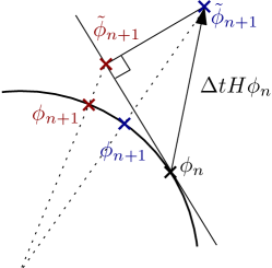
Figure 1: Update rule with the projected gradient, with the $\lambda$ term (red) and with the unprojected gradient, without the $\lambda$ term (blue).

For the FE and BE methods, a simple algebraic manipulation shows that one step of the method with the $\lambda$ term is equivalent to one step of the method without the $\lambda$ term, but with an effective $\Delta t$ modified as

$$\Delta_{t}^{\lambda,\text{FE}} =\frac{\Delta t}{1+\Delta t\lambda},$$ (4.11)

$$\Delta_{t}^{\lambda,\text{BE}} =\frac{\Delta t}{1-\Delta t\lambda}.$$ (4.12)

This is not true for the CN method, nor it is true when nonlinear terms are included. However, even in this case, the difference between including and not including the $\lambda$ term is $\mathcal{O}(\Delta t^{2})$, and their behavior is similar. Since the analysis of unprojected gradient methods is simpler, we focus on this here.

Then, these schemes can all be written in the form

$$\phi_{n+1} =\frac{A\phi_{n}}{\left\|A\phi_{n}\right\|},$$ (4.13)

where the matrix $A$ is given by

$$A^{\text{FE}} =I-\Delta tH,$$

$$A^{\text{BE}} =(I+\Delta tH)^{-1},$$

$$A^{\text{CN}} =(I+\frac{\Delta t}{2}H)^{-1}(I-\frac{\Delta t}{2}H).$$

The eigenvalues $\mu_{i}$ of $A$ are related to the eigenvalues $\lambda_{i}$ of $H$ by the following spectral transformation

$$\mu_{i}^{\text{FE}} =1-\Delta t\lambda_{i},$$

$$\mu_{i}^{\text{BE}} =\frac{1}{1+\Delta t\lambda_{i}},$$

$$\mu_{i}^{\text{CI}} =\frac{1-\frac{\Delta t}{2}\lambda_{i}}{1+\frac{\Delta t}{2}\lambda_{i}}.$$

We call this eigenvalue the amplification factor: if $\phi_{n}$ has eigencomponents $c_{n,i}=\left\langle v_{i},\phi_{n}\right\rangle$ on the eigenvector $v_{i}$ of $H$ and $\phi_{0}$ is normalized to $1$, then the iteration (4.13) can be solved as

$$c_{n,i}=\frac{\mu_{i}^{n}}{\sqrt{\sum_{i=1}^{N}|\mu_{i}^{n}c_{0,i}|^{2}}}\,c_{0,i}.$$

This iteration converges towards the eigenvector associated to the largest eigenvalue $\mu_{N}$ (in modulus) of $A$, if it is simple, with convergence rate $\mu_{N-1}/\mu_{N}$ . This is nothing but the classical power method for the computation of eigenvalues, with a spectral transformation from $H$ to $A$. Therefore we identify the FE method as a shifted power method, the BE method as a shift-and-invert approach, and the CN uses a generalized Cayley transform [10, 40].

From this we can readily see the properties of the different schemes. We make the assumption that either $\lambda_{1}$ is positive or that $\Delta t<\frac{1}{-\lambda_{1}}$ (for BE) and $\Delta t<\frac{2}{-\lambda_{1}}$ (for CN). If this condition is not verified, then the iteration will generally not converge towards an eigenvector associated with $\lambda_{1}$ because another eigenvalue than $\lambda_{1}$ will have a larger amplification factor. Under this assumption, we see that the BE and CN converge unconditionally, while FE only converges if

$$\Delta t<\frac{2}{\lambda_{N}}.$$

This is a CFL-like condition: when $H$ is the discretization of an elliptic operator, $\lambda_{N}$ will tend to infinity as the size of the basis increases, which will force FE to take smaller time steps.

The asymptotic convergence rate of these methods is $\frac{\mu_{N-1}}{\mu_{N}}$. While the FE method has a bounded convergence rate, imposed by $\lambda_{1},\lambda_{2}$ and $\lambda_{N}$, the BE and CN methods can be made to have an arbitrarily small convergence rate, by simply choosing $\Delta t$ arbitrarily close to $-\frac{1}{\lambda_{1}}$ (BE) or $-\frac{2}{\lambda_{1}}$ (CN). Since in practice $\lambda_{1}$ is unknown, it has to be approximated, for instance by $\lambda(\phi_{n})$. This yields the classical Rayleigh Quotient Iteration:

$$\phi_{n+1} =\frac{(H-\left\langle\phi_{n},H\phi_{n}\right\rangle)^{-1}\phi_{n}}{\left\|(H-\left\langle\phi_{n},H\phi_{n}\right\rangle)^{-1}\phi_{n}\right\|},$$

which is known to converge cubically. This iteration can also be seen as a Newton-like method.

From the previous considerations, it would seem that the BE and CN are infinitely superior to the FE method: even with a fixed stepsize, the BE and CN methods are immune to CFL-like conditions, and with an appropriately chosen stepsize, it can be turned into a superlinearly-convergent scheme. The first difficulty with this approach is that it is a linear strategy, only guaranteed to converge when close to the ground state. As is always the case with Newton-like methods, it requires a globalization strategy to be efficient and robust in the nonlinear setting. The second issue, is that the BE and CN method require the solution of the linear system $(H-\lambda(\phi_{n}))\tilde{\phi}_{n+1}=\phi_{n}$.

The difficulty of solving the system depends on the discretization scheme used. For localized basis schemes like the Finite Element Method, $H$ is sparse, and efficient direct methods for large scale sparse matrices can be used [39]. For the Fourier pseudo-spectral scheme, which we use in this paper, $H$ is not sparse, and only matrix-vector products are available efficiently through FFTs (a matrix-free problem). This means that the system has to be solved using an iterative method. Since it is a symmetric but indefinite problem, the solver of choice is MINRES [18], although the solver BICGSTAB has been used [7, 9]. The number of iterations of this solver will then grow when the grid spacing tends to zero, which shows that BE also has a CFL-like limitation. However, as is well-known, Krylov methods [39] only depend on the square root of the condition number for their convergence, as opposed to the condition number itself for fixed-point type methods [15, 46]. This explains why BE with a Krylov solver is preferred to FE in practice [7, 9].

Furthermore, preconditioners can be used to reduce this number of iterations [7, 9], e.g. with a simple preconditioner (one that is diagonal either in real or in Fourier space). This method is effective for many problems, but requires a globalization strategy, as well as an appropriate selection of parameters such as $\Delta t$ and the precision used to solve the linear system [7, 9]. Here, we propose a method that has all the advantages of BE (robust, Krylov-like dependence on the square root of the condition number, ability to use a preconditioner), but is explicit, converges faster than BE, and has no free parameter (no fine-tuning is necessary).

5 The Preconditioned nonlinear Gradient (PG) and Conjugate Gradient (PCG) methods

5.1 The gradient method

The previous approaches usually employed in the literature to compute the ground states of the Gross-Pitaevskii equation are all based on implicit discretizations of the imaginary-time equation (4.4). As such, these methods come from PDE theory and lack the insight of minimization algorithms. The difficulty of applying classical minimization algorithms comes from the spherical constraints. However, the general theory of optimization algorithms on Riemannian manifolds has been developed extensively in [2, 32], where the authors derive constrained analogues of gradient, conjugate gradient and Newton algorithms. This is the approach we follow here, and employ a preconditioned conjugate gradient method on the manifold $\mathcal{S}$.

In this section, we work with an arbitrary symmetric positive definite preconditioner $P$. The choice of $P$ will be discussed later in subsection 5.5. The (projected, preconditioned) gradient method for the minimization of $E$ on $\mathcal{S}$ is the update

$$\tilde{\phi}_{n+1} =\phi_{n}-\alpha_{n}P\left(H_{\phi_{n}}\phi_{n}-\lambda_{n}\phi_{n}\right),\quad\phi_{n+1}={\tilde{\phi}_{n+1}}/{\left\|\tilde{\phi}_{n+1}\right\|},$$ (5.14)

where $\lambda_{n}=\lambda(\phi_{n}).$ We reformulate this equation as

$$\phi_{n+1} =\cos(\theta_{n})\phi_{n}+\sin(\theta_{n})\frac{p_{n}}{\left\|p_{n}\right\|},\quad\text{with}\quad p_{n}={d_{n}-\operatorname{Re}\left\langle d_{n},\phi_{n}\right\rangle\phi_{n}},$$ (5.15)

where $d_{n}=-Pr_{n}$ is the descent direction, equal to the negative of the preconditioned residual $r_{n}=H_{\phi_{n}}\phi_{n}-\lambda(\phi_{n})\phi_{n}$. The equations (5.14) and (5.15) are equivalent when $\theta_{n}$ or $\alpha_{n}$ is small enough, with a one-to-one correspondance between $\theta_{n}$ and $\alpha_{n}$. To first order, we have: $\alpha_{n}=\theta_{n}\left\|p_{n}\right\|$.

Without preconditioner, this method, summarized in Algorithm 1, is identical to the FE method (4.8).

while not converged do

       $\lambda_{n}=\lambda(\phi_{n})$

      $r_{n}=H_{\phi_{n}}\phi_{n}-\lambda_{n}\phi_{n}$

      $d_{n}=-Pr_{n}$

      $p_{n}={d_{n}-\operatorname{Re}\left\langle d_{n},\phi_{n}\right\rangle\phi_{n}}$

      $\theta_{n}=\operatorname*{arg\,min}_{\theta}E\left(\cos(\theta)\phi_{n}+\sin(\theta){p_{n}}/{\left\|p_{n}\right\|}\right)$

      $\phi_{n+1}=\cos(\theta_{n})\phi_{n}+\sin(\theta_{n}){p_{n}}/{\left\|p_{n}\right\|}$

      $n=n+1$

end while

Algorithm 1 The gradient method

To choose the parameter $\theta_{n}$, a number of strategies are possible. We first show that, when $\theta_{n}$ is small enough, the gradient method decreases the energy.

Expanding $\phi_{n+1}$ up to second-order in $\theta_{n}$, we obtain

$$\phi_{n+1} =\left(1-\frac{\theta_{n}^{2}}{2}\right)\phi_{n}+\theta_{n}\frac{p_{n}}{\left\|p_{n}\right\|}+\mathcal{O}(\theta_{n}^{3}),$$ (5.16)

and therefore

$$E(\phi_{n+1}) =E(\phi_{n})+\frac{\theta_{n}}{\left\|p_{n}\right\|}\operatorname{Re}\left\langle\nabla E(\phi_{n}),p_{n}\right\rangle+\frac{1}{2}\frac{\theta_{n}^{2}}{\left\|p_{n}\right\|^{2}}\left[\nabla^{2}E(\phi_{n})[p_{n},p_{n}]-\lambda_{n}\left\|p_{n}\right\|^{2}\right]+\mathcal{O}(\theta_{n}^{3}).$$ (5.17)

We now compute the first-order variation

$$\operatorname{Re}\left\langle\nabla E(\phi_{n}),p_{n}\right\rangle =\frac{\operatorname{Re}\left\langle\nabla E(\phi_{n}),d_{n}-\operatorname{Re}\left\langle d_{n},\phi_{n}\right\rangle\phi_{n}\right\rangle}{\left\|{d_{n}-\operatorname{Re}\left\langle d_{n},\phi_{n}\right\rangle\phi_{n}}\right\|}=\frac{\operatorname{Re}\left\langle r_{n},d_{n}\right\rangle}{\left\|{d_{n}-\operatorname{Re}\left\langle d_{n},\phi_{n}\right\rangle\phi_{n}}\right\|}$$

$$=-\frac{\left\langle r_{n},Pr_{n}\right\rangle}{\left\|{d_{n}-\operatorname{Re}\left\langle d_{n},\phi_{n}\right\rangle\phi_{n}}\right\|}.$$

Since $P$ was assumed to be positive definite, this term is always negative so that the algorithm decreases the energy when $\theta_{n}$ is chosen small enough. Since $p_{n}$ is orthogonal to $\phi_{n}$, the second-order term $\nabla^{2}E(\phi_{n})[p_{n},p_{n}]-\lambda_{n}\left\|p_{n}\right\|^{2}$ is guaranteed to be positive when $\phi_{n}$ is close to a minimizer by the second-order optimality conditions.

Therefore, a basic strategy is to choose $\theta_{n}$ fixed and small enough so that the energy decreases. A better one is to choose $\theta_{n}$ adaptively. For instance, we could perform the linesearch

$$\theta_{n}=\operatorname*{arg\,min}_{\theta}E\left(\cos(\theta)\phi_{n}+\sin(\theta)\frac{p_{n}}{\left\|p_{n}\right\|}\right).$$ (5.18)

Since $E(\theta)$ is not a quadratic function, this is a nonlinear one-dimensional minimization problem, generally requiring many evaluations of $E(\theta)$ to converge to a minimum. However, many of the computations for the evaluation of $E(\theta)$, including all that require FFTs, can be pre-computed. Since the FFT step is the dominant one in the computation of the energy, the evaluation of $E(\theta)$ at many points is not much more costly than the evaluation at a single point. Therefore it is feasible to use a standard one-dimensional minimization routine.

Alternatively, we can obtain a simple and cheap approximation by minimizing the second-order expansion of $E$ in $\theta_{n}$. We expect this to be accurate when $\theta_{n}$ is small, which is the case close to a minimizer. Minimizing (5.17) with respect to $\theta_{n}$ yields

$$\theta_{n}^{\rm opt} =\frac{-\operatorname{Re}\left\langle\nabla E(\phi_{n}),p_{n}\right\rangle\left\|p_{n}\right\|}{\operatorname{Re}\left[\nabla^{2}E(\phi_{n})[p_{n},p_{n}]-\lambda_{n}\right]}.$$ (5.19)

As we have seen, the numerator is always positive, and the denominator is positive when $\phi_{n}$ is close enough to a minimizer. In our implementation, we compute the denominator, and, if it is positive, we use $\theta_{n}^{\rm opt}$ as a trial stepsize. If not, we use some default positive value. If the energy of $\phi_{n+1}$ using this trial stepsize is decreased, we accept the step. If the energy is not decreased, we reject the step, decrease the trial stepsize, and try again, until the energy is decreased (which is mathematically ensured when $\theta_{n}$ is small enough). Alternatively, we can use Armijo or Wolfe conditions as criterion to accept or reject the stepsize, or even use the full line search (5.18). The evaluation of the energy at multiple values of $\theta$ do not require more Fourier transforms than at only one point, but only more computations of the nonlinear term, so that a full line search is not much more costly than the heuristic outlined above. In our tests however, the heuristic above was sufficient to ensure fast convergence, and a full line search only marginally improved the number of iterations. Therefore, we simply use the heuristic in the numerical results of Section 6.

Let us note that under reasonable assumptions on the structure of critical points and on the stepsize choice, there are various results on the convergence of this iteration to a critical point (see [2] and references therein).

5.2 The conjugate gradient method

The conjugate gradient method is very similar, but uses an update rule of the form

$$d_{n} =-Pr_{n}+\beta_{n}p_{n-1}$$ (5.20)

instead of simply $d_{n}=-Pr_{n}$. This is justified when minimizing unconstrained quadratic functionals, where the formula

$$d_{n}=-Pr_{n}+\beta_{n}d_{n-1},\quad\text{with}\quad\beta_{n}=\frac{\left\langle r_{n},Pr_{n}\right\rangle}{\left\langle r_{n-1},Pr_{n-1}\right\rangle},$$ (5.21)

yields the well-known PCG method to solve linear systems. For nonlinear problems, different update formulas can be used, all equivalent in the linear case. Equation (5.21) is known as the Fletcher-Reeves update. Another popular formula is the Polak-Ribière choice $\beta=\max(\beta^{\textrm{PR}},0)$, where

$$\beta^{\textrm{PR}} =\frac{\left\langle r_{n}-r_{n-1},Pr_{n}\right\rangle}{\left\langle r_{n-1},Pr_{n-1}\right\rangle}.$$ (5.22)

We use $\beta=\max(\beta^{\textrm{PR}},0)$, which is equivalent to restarting the CG method (simply using a gradient step) when $\beta^{\textrm{PR}}<0$ and is a standard choice in nonlinear CG methods. For the justification of the CG method for constrained minimization, see [2, 32].

while not converged do

       $\lambda_{n}=\lambda(\phi_{n})$

      $r_{n}=H_{\phi_{n}}\phi_{n}-\lambda_{n}\phi_{n}$

      $\beta_{n}={\left\langle r_{n}-r_{n-1},Pr_{n}\right\rangle}/{\left\langle r_{n-1},Pr_{n-1}\right\rangle}$

      $\beta_{n}=\max(\beta_{n},0)$

      $d_{n}=-Pr_{n}+\beta p_{n-1}$

      $p_{n}=d_{n}-\operatorname{Re}\left\langle d_{n},\phi_{n}\right\rangle\phi_{n}$

      $\theta_{n}=\operatorname*{arg\,min}_{\theta}E\left(\cos(\theta)\phi_{n}+\sin(\theta){p_{n}}/{\left\|p_{n}\right\|}\right)$

      $\phi_{n+1}=\cos(\theta_{n})\phi_{n}+\sin(\theta_{n}){p_{n}}/{\left\|p_{n}\right\|}$

      $n=n+1$

end while

Algorithm 2 The conjugate gradient method

The CG algorithm is presented in Algorithm 2. In contrast with the gradient algorithm, the quantity $\operatorname{Re}\left\langle\nabla E(\phi_{n}),p_{n}\right\rangle$ does not have to be negative, and $p_{n}$ might not be a descent direction: even with a small stepsize, the energy does not have to decrease at each step. To obtain a robust minimization method, we enforce energy decrease to guarantee convergence. Therefore, our strategy is to first check if $p_{n}$ is a descent direction by computing $\operatorname{Re}\left\langle\nabla E(\phi_{n}),p_{n}\right\rangle$. If $p_{n}$ is not a descent direction, we revert to a gradient step, which we know will decrease the energy, else, we choose $\theta_{n}$ as in (5.19), and use the same stepsize control as in the gradient algorithm.

In our numerical tests, we observe that these precautions of checking the descent direction and using a stepsize control mechanism are useful in the first stage of locating the neighborhood of a minimum. Once a minimum is approximately located, $p_{n}$ is always a descent direction and the stepsize choice (5.19) always decreases the energy.

5.3 Stopping criteria

A common way to terminate the iteration (in the BE schemes) is to use the stopping criterion

$$\phi_{\rm err}^{n,\infty}\mathrel{\mathop{\mathchar 58\relax}}=\|\phi_{n+1}-\phi_{n}\|_{\infty}\leq\varepsilon.$$ (5.23)

This can be problematic because the minima are generally not isolated but form a continuum due to symmetries (for instance, complex phase or rotational invariance), and this criterion might be too restrictive. A more robust one is based on the norm of the symmetry-covariant residual

$$r^{n,\infty}_{\rm err}\mathrel{\mathop{\mathchar 58\relax}}=\|r_{n}\|_{\infty}=\|H_{\phi_{n}}\phi_{n}-\lambda_{n}\phi_{n}\|_{\infty}\leq\varepsilon.$$ (5.24)

or the symmetry-invariant energy difference

$$\mathcal{E}^{n}_{\rm err}\mathrel{\mathop{\mathchar 58\relax}}=|E(\phi_{n+1})-E(\phi_{n})|\leq\varepsilon.$$ (5.25)

This third one converges more rapidly than the two previous ones: as is standard in optimization, when $\phi^{*}$ is a minimum of the constrained minimization problem and $\phi\in\mathcal{S}$, then

$$E(\phi)-E(\phi^{*})=\mathcal{O}(\|\phi-\phi^{*}\|^{2}).$$

This is consistent with our results in Figure 7.

In the current paper, we always use the energy based stopping criterion (5.25): for the 2D and 3D cases, a criteria based on $\phi^{n,\infty}_{\rm err}$ or $r^{n,\infty}_{\rm err}$ can lead to long computational times, most particularly for large rotations $\omega$, even without changing the energy (see the example in subsection 6.2).

5.4 Convergence analysis

A full analysis of the convergence properties of our methods is outside the scope of this paper, but we give in this section some elementary properties, and heuristics to understand their asymptotic performance.

Based on the expansion of the energy (5.17) as a function of $\theta$ for the gradient method, it is straightforward to prove that, when $E$ is bounded from below and the stepsize $\theta$ is chosen optimally, the norm of the projected gradient $H_{\phi_{n}}\phi_{n}-\lambda_{n}\phi_{n}$ converges to $0$. Convergence guarantees for the conjugate gradient method are harder, but can still be proven under a suitable restart strategy that ensures that the energy always decreases fast enough (for instance, the Armijo rule).

With additional assumptions on the non-degeneracy of critical points, we can even prove the convergence of $\phi_{n}$ to a critical point, that will generically be a local minimum. However, the question of the precise convergence speed of the gradient and conjugate gradient algorithms we use is problematic, because of three factors: the constraint $\left\|\phi\right\|=1$, the non-quadraticity of $E$, and the presence of a preconditioner. To our knowledge, no asymptotically optimal bound for this problem has been derived. Nevertheless, based on known results about the convergence properties of the conjugate gradient method for preconditioned linear systems on the one hand [39], and of gradient methods for nonlinear constrained minimization [2] on the other, it seems reasonable to expect that the convergence will be influenced by the properties of the operator

$$M=(1-\phi\phi^{*})P(\nabla^{2}E(\phi)-\lambda I)(1-\phi\phi^{*}),$$ (5.26)

where $\phi$ is the minimum and $\lambda=\lambda(\phi)$. This operator admits $0$ as its lowest eigenvalue, associated with the eigenvector $\phi$. It is reasonable to expect that the convergence rate will be determined by a condition number $\sigma$ equals to the ratio of the largest to the lowest non-zero eigenvalue of this operator. As is standard for linear systems, we also expect that the number of iterations to achieve a given tolerance will behave like $\sqrt{\sigma}$ for the conjugate gradient algorithm, and $\sigma$ for the gradient algorithm. As we will see in Section 6, this is verified in our tests.

The Hessian operator $\nabla^{2}E(\phi)$, which includes a Laplace operator, is not bounded. Correspondingly, on a given discretization domain, when the grid is refined, the largest eigenvalues of this operator will tend to $+\infty$. For a linear meshsize $h$, the eigenvalues of $\nabla^{2}E(\phi)$ will behave as $\mathcal{O}(h^{-2})$. This is another instance of the CFL condition already seen in the discretization of the imaginary time equation. The Hessian $\nabla^{2}E$ also includes a potential term $V$, which is often confining and therefore not bounded, such as the classical harmonic potential $V(\textbf{x})=|\textbf{x}|^{2}$, or more generally confining potentials whose growth at infinity is like $|\textbf{x}|^{p}$. for some $p>0$ Thus, even with a fixed meshsize $h$ on a domain $[-L,L]^{d}$, when $L$ is increased, so will the largest eigenvalues of $\nabla^{2}E(\phi)$, with a $\mathcal{O}(L^{p})$ growth. When a (conjugate) gradient method is used without preconditioning, the convergence will be dominated by modes associated with largest eigenvalues of $\nabla^{2}E$. This appears in simulations as high-frequency oscillations and localization at the boundary of the domain of the residual $r_{n}$.

To remedy these problems and achieve a good convergence rate, adequate preconditioning is crucial.

5.5 Preconditioners

We consider the question of building preconditioners $P$ for the algorithms presented above. In the schemes based on the discretization of the gradient flow, preconditioning is naturally needed when solving linear systems by iterative methods. In the gradient and conjugate gradient optimization schemes, it appears as a modification of the descent direction to make it point closer to the minimum:

$$d_{n}\mathrel{\mathop{\mathchar 58\relax}}=-P(H_{\phi_{n}}\phi_{n}-\lambda_{n}\phi_{n}).$$ (5.27)

In both cases, the preconditioning matrix should be an approximation of the inverse of the Hessian matrix of the problem.

Kinetic energy preconditioner

One of these approximations is to use only the kinetic energy term

$$P_{\Delta} =(\alpha_{\Delta}-\Delta/2)^{-1},$$ (5.28)

where $\alpha_{\Delta}$ is a positive shifting constant to get an invertible operator, and $I$ is the identity operator. This has been called a “Sobolev gradient” in [29] because it is equivalent to taking the gradient of the energy in the Sobolev $H^{1}$-norm (with $\alpha_{\Delta}=1/2$). In the framework of the BESP scheme for the GPE with Krylov solver, a similar preconditioner has been proposed in [7], $\alpha_{\Delta}$ being the inverse of the time step $\Delta t$ of the semi-implicit Euler scheme. A closely-related variant is standard in plane-wave electronic structure computation [47], where it is known as the Tetter-Payne-Allan preconditioner [42]. This preconditioner is diagonal in Fourier space and can therefore be applied efficiently in our pseudo-spectral approximation scheme. On a fixed domain $[-L,L]^{d}$, the effect of this preconditioner is to make the number of iterations independent from the spatial resolution $h$, because $P\nabla^{2}E(\phi)$, seen as an operator on the space of functions on $[-L,L]^{d}$, will be equal to the identity plus a compact operator. This is supported by numerical experiments in Section 6. However, this operator is not bounded in the full domain $\mathbb{R}^{d}$. Therefore, as $L$ increases, so will the largest eigenvalues of $P\nabla^{2}E(\phi)$. For a potential $V$ that grows at infinity like $|\mathbf{x}|^{p}$, the largest eigenvalues of $P\nabla^{2}E(\phi)$ are $\mathcal{O}(L^{p})$, resulting in an inefficient preconditioner. Similarly, when $\eta$ is large, the nonlinear term becomes dominant, and the kinetic energy preconditioner is inefficient.

The choice of $\alpha_{\Delta}$ is a compromise: if $\alpha_{\Delta}$ is too small, then the preconditioner will become close to indefinite, which can produce too small eigenvalues in the matrix (5.26) and hamper convergence. If $\alpha_{\Delta}$ is too big, then the preconditioner does not act until very large frequencies, and large eigenvalues result. We found that a suitable adaptive choice, that has consistently good performance and avoids free parameters, is

$$\alpha_{\Delta}=\tilde{\lambda}_{n}\mathrel{\mathop{\mathchar 58\relax}}=\int\bigg{(}\frac{1}{2}|\nabla\phi_{n}|^{2}+V|\phi_{n}|^{2}+\eta|\phi_{n}|^{4}\bigg{)}d\mathbf{x}>0$$ (5.29)

which is a positive number that represents the characteristic energy of $\phi_{n}$. We use this choice for our numerical simulations.

Potential energy preconditioner

Another natural approach is to use the potential energy term for the preconditioner:

$$P_{V} =(\alpha_{V}+V+\eta|\phi_{n}|^{2})^{-1}.$$ (5.30)

This preconditioner is diagonal in real space and can therefore be applied efficiently. Dual to the previous case, this preconditioner has a stable performance when the domain and $\eta$ are increased, but deteriorates as the spatial resolution is increased. Such a preconditioner has been used in [7] when the gradient flow for the GPE is discretized through a BE scheme, leading then to a Thomas-Fermi preconditioner. In this study, the parameter $\alpha_{V}$ was $1/\Delta t$. As in the kinetic energy case, we found it efficient to use $\alpha_{V}=\tilde{\lambda}_{n}$, and we will only report convergence results for this choice of parameter.

Combined preconditioner

In an attempt to achieve a stable performance independent of the size of the domain or the spatial resolution, we can define the combined preconditioners

$$P_{\textrm{C}_{1}} =P_{V}P_{\Delta},\quad P_{\textrm{C}_{2}}=P_{\Delta}P_{V}$$ (5.31)

or a symmetrized version

$$P_{\textrm{C}} =P_{V}^{1/2}P_{\Delta}P_{V}^{1/2}.$$ (5.32)

With these preconditioners, $P\nabla^{2}E(\phi)$ is bounded as an operator on $L^{2}(\mathbb{R}^{d})$ (this can be proven by writing explicitly its kernels in Fourier space and then using Schur’s test). However, we found numerically that this operator is not bounded away from zero, and has small eigenvalues of size $\mathcal{O}(L^{-p}+h^{2})$. Therefore, the conditioning deteriorates as both the spatial resolution and the size of the domain increase.

In summary, for a spatial resolution $h$ and a domain size $L$, the asymptotic condition numbers of the preconditioned Hessian with these preconditioners are

$$\begin{array}[]{l}\kappa_{\Delta}=\mathcal{O}(L^{p}),\\ \kappa_{V}=\mathcal{O}(h^{-2}),\\ \kappa_{\textrm{C}}=\mathcal{O}\left(\frac{1}{L^{-p}+h^{2}}\right)=\mathcal{O}(\min(L^{p},h^{-2})).\end{array}$$ (5.33)

Therefore, the combined preconditioners act asymptotically as the best of both the kinetic and potential preconditioners. However, they might not be more efficient in the pre-asymptotic regime and require additional Fourier transforms.

Computational efficiency

The application the operator $P_{V}$ is almost free (since it only requires a scaling of $\phi$), but the naive application of $P_{\Delta}$ requires a FFT/IFFT pair. However, since we apply the preconditioners after and before an application of the Hamiltonian, we can reuse FFT and IFFT computations, so that the application of $P_{\Delta}$ does not require any additional Fourier transform. Similarly, the use of $P_{\rm C_{1}}$ and $P_{\rm C_{2}}$ only require one additional Fourier transform per iteration, and that of the symmetrized version $P_{\rm C}$ two.

In summary, the cost in terms of Fourier transforms per iteration for the rotating GPE model is

• no preconditioner: 3 FFTs/iteration (get the Fourier transform of $\phi$, and two IFFTs to compute $\Delta\phi$ and $L_{z}\phi$ respectively),

• $P_{\Delta}$ or $P_{V}$: 3 FFTs/iteration,

• non-symmetric combined $P_{\rm C_{1}}$ or $P_{\rm C_{2}}$: 4 FFTs/iteration,

• symmetric combined $P_{\rm C}$: 5 FFTs/iteration.

Note that this total might be different for another type of GPE model e.g. when a nonlocal dipole-dipole interaction is included [9, 16].

As we will see in Section 6, all combined preconditioners have very similar performance, but the symmetrized one might be more stable in some circumstances. A theoretical explanation of these observations, and in particular of the effect of a non-symmetric preconditioner is, to the best of our knowledge, still missing.

6 Numerical results

We first introduce some notations. When we combine one of the preconditioners $P_{\nu}$ ($\nu=I$, $\Delta$, $V$, C, ${\rm C_{1}}$, ${\rm C_{2}}$) (5.28)-(5.32) with the gradient algorithm (Alg: 1), we denote the resulting methods by PG_ν. Similarly, we denote by PCG_ν if the preconditioned conjugate gradient algorithm (Alg: 2) was applied. In the following, we denote by $\#\rm iter$ the number of global iterations for an iterative algorithm to get the converged solution with an a priori tolerance $\varepsilon$ with respect to the stopping criterion (5.25).

Concerning the BESP schemes (4.6) and (4.9), at each outer iteration $n$, one needs to solve an implicit system with the operator $(1/\Delta t+H_{\bm{\phi}_{n}})$. We use a Krylov subspace iterative solver (MINRES here) with one of the preconditioners $P_{\nu}$ ($\nu=I,\Delta,V,\textrm{C}$) (5.28)-(5.31) to accelerate the number of inner iterations [7]. The preconditioned BESP schemes is then denoted by BE_ν, according to the chosen preconditioner. The number of iterations reported is equal to the sum of the inner iterations over the outer iterations.

In the following numerical experiments, we consider two types of trapping potential $V(\mathbf{x})$: the harmonic plus lattice potential [13]

$$V(\mathbf{x})=V_{d}^{0}(\mathbf{x})+\left\{\begin{array}[]{l}\kappa_{x}\sin^{2}(q_{x}x^{2}),\\[3.99994pt] \sum_{\nu=x,y}\kappa_{\nu}\sin^{2}(q_{\nu}\nu^{2}),\\[3.99994pt] \sum_{\nu=x,y,z}\kappa_{\nu}\sin^{2}(q_{\nu}\nu^{2}),\end{array}\right.\quad{\rm with}\quad V_{d}^{0}(\mathbf{x})=\left\{\begin{array}[]{ll}\gamma_{x}^{2}x^{2},&d=1,\\[3.99994pt] \sum_{\nu=x,y}\gamma_{\nu}\nu^{2},&d=2,\\[3.99994pt] \sum_{\nu=x,y,z}\gamma_{\nu}\nu^{2},&d=3,\end{array}\right.$$ (6.34)

and the harmonic plus quartic potential for $d=2,3$ [28, 29, 46]

$$V(\mathbf{x})=(1-\alpha)V_{2}^{0}(\mathbf{x})+\frac{\kappa\,(x^{2}+y^{2})^{2}}{4}+\left\{\begin{array}[]{ll}0,&d=2,\\[3.99994pt] \gamma_{z}^{2}\,z^{2},&d=3.\end{array}\right.$$ (6.35)

Moreover, unless stated otherwise, we take the initial data as the Thomas Fermi approximation [7, 13]:

$$\phi_{0}=\frac{\phi^{\rm TF}_{g}}{\|\phi^{\rm TF}_{g}\|},\qquad{\rm with}\qquad\phi^{\rm TF}_{g}(\mathbf{x})=\left\{\begin{array}[]{ll}\sqrt{\big{(}\mu_{g}^{\rm TF}-V(\mathbf{x})\big{)}/\eta},&V(\mathbf{x})<\mu_{g}^{\rm TF},\\[3.99994pt] 0,&{\rm otherwise},\end{array}\right.$$ (6.36)

where

$$\mu_{g}^{\rm TF}=\frac{1}{2}\left\{\begin{array}[]{ll}(3\eta\gamma_{x})^{2/3},&d=1,\\ (4\eta\gamma_{x}\gamma_{y})^{1/2},&d=2,\\ (15\eta\gamma_{x}\gamma_{y}\gamma_{z})^{2/5},&d=3.\end{array}\right.$$ (6.37)

The algorithms were implemented in Matlab (Release 8.5.0).

6.1 Numerical results in 1D

Here, $V(\mathbf{x})$ is chosen as the harmonic plus lattice potential (6.34) with $\gamma_{x}=1$, $k_{x}=25$ and $q_{x}=\frac{\pi}{2}.$ The computational domain and mesh size are respectively denoted as $\mathcal{D}=[-L,L]$ and $h$. In addition, to compare with the common existing method BESP, we choose the stopping criteria (5.25) with $\varepsilon=10^{-14}$ all through this section. For BESP, we choose $\Delta t=0.01$ unless specified otherwise, and fix the error tolerance for the inner loop to $10^{-10}$. Other values of the error tolerance were also tried, but this choice was found to be representative of the performance of BESP.

Example 6.1.

We first compare the performance of various solvers without preconditioning in a simple case. We choose $L=16$ and $\eta=250$, and varying mesh sizes. We compare the method BE_I given by (4.9), BE${}_{I}^{\lambda}$ given (4.6), and the gradient and conjugate gradient algorithms in Figure 2. The difference between methods BE_I and BE${}_{I}^{\lambda}$ is the inclusion of the chemical potential in the discretized gradient flow: we showed in Section 4 that both were equivalent for linear problems up to a renormalization in $\Delta t$. We see here that this conclusion approximately holds even in the nonlinear regime ($\eta\neq 0$), with both methods performing very similarly until $\Delta t$ becomes large, at which point the BE${}_{I}^{\lambda}$ effectively uses a constant stepsize (see (4.12)), while the large timestep in BE_I makes the method inefficient. In this case, $\lambda_{1}$ is positive, so that both methods converge to the ground state even for a very large $\Delta t$. Overall we see that the optimum number of iterations is achieved for a value of $\Delta t$ of about $0.01$, which we keep in the following tests to ensure a fair comparison. We also use the BE^λ variant in the following tests.

For modest values of the discretization parameter $h$, the Backward Euler methods are less efficient than the gradient method (which can be interpreted as a Forward Euler iteration with adaptive stepsize). As $h$ is decreased, the conditioning of the problem increases as $h^{-2}$. The gradient/Forward Euler method is limited by its CFL condition, and its number of iterations grows like $h^{-2}$, as can readily be checked in Figure 2. The Backward Euler methods, however, use an efficient Krylov solver that is only sensitive to the square root of the conditioning, and its number of iterations grows only like $h^{-1}$. Therefore it become more efficient than the gradient/Forward Euler method.

The conjugate gradient method is always more efficient than the other methods by factors varying between one and two orders of magnitude. Its efficiency can be attributed to the combination of Krylov-like properties (as the Backward Euler method, its iteration count displays only a $h^{-1}$ growth) and optimal stepsizes.

  

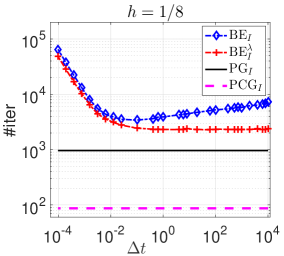
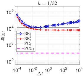
Figure 2: Example 6.1. Number of iterations to converge for different methods and different stepsizes, with different values of the discretization parameter $h$.

Example 6.2.

We compare now the performance of the (conjugate) gradient method with different preconditioners. To this end, we consider the algorithms PG_ν and PCG_ν with $\nu=\Delta,V,{\rm C},{\rm C_{1}},{\rm C_{2}}.$ The computational parameters are chosen as $L=128$ and $h=\frac{1}{64}$, respectively. Fig. 3 shows the iteration number $\#\rm iter$ for these schemes and different values of the nonlinearity strength $\eta$. From this figure and other numerical results not shown here, we can see that: (i) For each fixed preconditioner, the PCG schemes works better than the PG schemes; (ii) the combined preconditioners all work equally well, and bring a reduction in the number of iteration, at the price of more Fourier transforms.

  

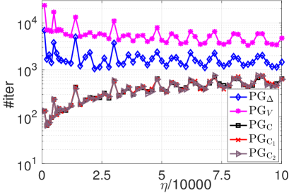
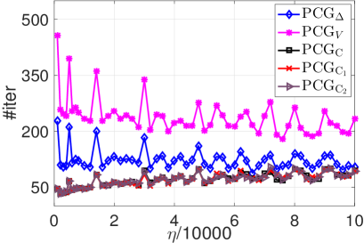
Figure 3: Example 6.2. Number of iterations of PG_ν and PCG_ν ($\nu=\Delta,V,{\rm C},{\rm C_{1}},{\rm C_{2}}$) to converge, for different nonlinear strengths $\eta$.

Example 6.3.

In this example, we compare the performance of PG_ν, PCG_ν and BE_ν ($\nu=I,\Delta,V,\textrm{C}$) with respect to different domain and mesh sizes. To this end, we fix $\eta=250$. Fig. 4 shows the total iteration number for these schemes with different $L$ and $h$. From this figure and additional numerical results not shown here for brevity, we see that: (i) Preconditioned solvers outperform unpreconditioned solvers; (ii) The potential preconditioner $P_{V}$ (5.30) makes the solver mainly depend on the spatial resolution $h$, while the kinetic potential preconditioner $P_{\Delta}$ (5.28) prevents the deterioration as $h$ decreases for a fixed $L$, consistent with the theoretical analysis in subsection 5.5; (iii) The deterioration is less marked for Krylov-based methods (BE and PCG) than for the PG method, because Krylov methods only depends on the square root of the condition number (iv) The combined preconditioner $P_{\rm C}$ (5.31) makes the solvers almost independent of both the parameters $h$ and $L$, although we theoretically expect a stronger dependence. We attribute this to the fact that we start with a specific initial guess that does not excite the slowly convergent modes enough to see the dependence on $h$ and $L$; (v) For each solver, the combined preconditioner $P_{\rm C}$ performs best. Usually, PCG_C is the most efficient algorithm, followed by PG_C, and finally BE_C.

	BE	PG	PCG
$P_{I}$
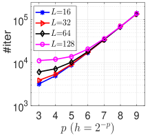
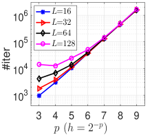
$P_{V}$
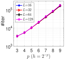
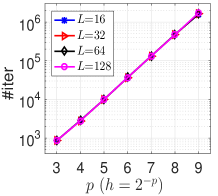
$P_{\Delta}$
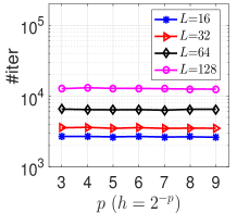
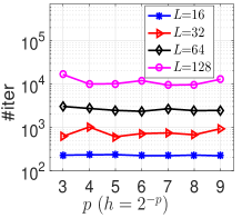
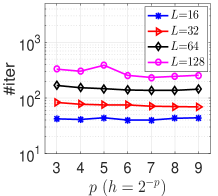
$P_{\rm C}$

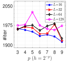
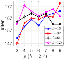
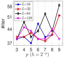
Figure 4: Example 6.3. Number of iterations to converge for BE_ν, PG_ν and PCG_ν for $\nu=I,V,\Delta,\textrm{C}$, vs. the mesh refinement $h$.

Example 6.4.

We investigate further the performance of PCG_C and PG_C with different nonlinear interaction strenghts $\eta$. To this end, we take $L=128$ and different discretization parameters $h$. We vary the nonlinearity from $\eta=0$ to $\eta=10^{5}.$ Fig. 5 depicts the corresponding iteration numbers to converge. We could clearly see that: (i) The iteration counts for both methods are almost independent on $h$, but both depend on the nonlinearity $\eta$; PCG_C depends slightly on $\eta$ while PG_C is more sensitive; (ii) For fixed $\eta$ and $h$, PCG_C converges much faster than PG_C.

 

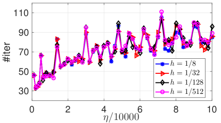
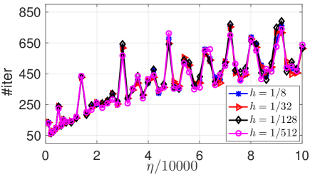
Figure 5: Example 6.4. Number of iterations to converge for PCG_C (left) and PG_C (right) with $L=128$, and various values of $h$ and $\eta$.

From examples 6.2–6.4, we see that PCG_C, i.e. PCG with combined symmetric preconditioner $P_{\rm C}$ (5.31) is the best solver. Hereafter, unless stated, we use PCG_C as the default solver to compute the ground states.

6.2 Numerical results in 2D

Here, we choose $V(\mathbf{x})$ as the harmonic plus quartic potential (6.35) with $\gamma_{x}=\gamma_{y}=1$, $\alpha=1.2$ and $\kappa=0.3.$ The computational domain and mesh sizes are chosen respectively as $\mathcal{D}=[-16,16]^{2}$ and $h=\frac{1}{16}.$

First, we test the evolution of the three errors (5.23)–(5.25) as the algorithm progresses. To this end, we take $\eta=1000$ and $\omega=3.5$ as example. Fig. 6 plots the $\phi^{n,\infty}_{\rm err}$, $r^{n,\infty}_{\rm err}$ and $\mathcal{E}^{n}_{\rm err}$ errors with respect to the iteration number. We can see clearly that $\mathcal{E}^{n}_{\rm err}$ converges faster the other two indicators, as expected. Considering $\phi^{n,\infty}_{\rm err}$ or $r^{n,\infty}_{\rm err}$ with an improper but relative large tolerance would require a very long computational time to converge even if the energy would not change so much. This is most particularly true for large values of $\omega$. In all the examples below, unless stated, we fix $\mathcal{E}^{n}_{\rm err}$ (5.25) with $\varepsilon=10^{-12}$ to terminate the code.

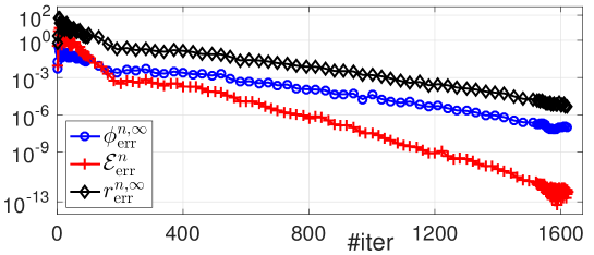
Figure 6: Evolution of the errors vs. the total number of iterations.

Example 6.5.

In this example, we compare the performance of PCG_C and PG_C for the 2D rotating case. To this end, $V(\mathbf{x})$ is chosen as the harmonic plus lattice potential (6.34) with $\gamma_{x}=\gamma_{y}=1$, $k_{x}=k_{y}=25$ and $q_{x}=q_{y}=\frac{\pi}{2}$. The computational domain and mesh sizes are chosen respectively as $\mathcal{D}=[-32,32]^{2}$ and $h=\frac{1}{8}$. Fig. 7 (left) shows the iteration number of PCG_C and PG_C vs. different values of $\eta$ for $\omega=0$, while Fig. 7 (right) reports the number of iterations of PCG_C with respect to $\eta$ and $\omega$. From this figure, we can see that: (i) Similarly to the 1D case, PCG_C outperforms PG_C; (ii) For $\omega=0$, the iteration number for PCG_C would oscillate in a small regime, which indicates the very slight dependence with respect to the nonlinearity strength $\eta$. When $\omega$ increases, the number of iterations increases for a fixed $\eta$. Meanwhile, the dependency on $\eta$ becomes stronger as $\omega$ increases. Let us remark here that it would be extremely interesting to build a robust preconditioner including the rotational effects to get a weaker $\omega$-dependence in terms of convergence.

  

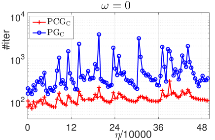
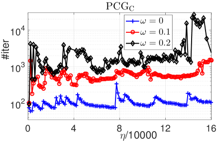
Figure 7: Exemple 6.5. Number of iterations for PCG_C and PG_C for $\omega=0$ (left) and PCG_C for different $\omega$ (right) vs. $\eta.$

Example 6.6.

Following the previous example, here we compare the performance of PCG_C and PCG${}_{\rm C_{1}}$ for different values $\omega$. To this end, we fix $\eta=1000$ and vary $\omega$ from 0 to 3.5. Fig. 8 illustrates the number of iterations of these method vs. different values of $\omega$ and there corresponding energies. From this figure and other experiments now shown here, we see that (i) All the methods converge to the stationary state with same energy; (ii) The symmetrized preconditioner has more stable performance than the non-symmetric version, a fact we do not theoretically understand.

    

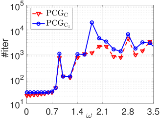
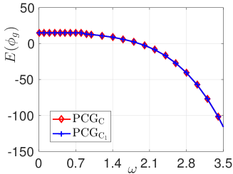
Figure 8: Exemple 6.6. Number of iterations for PCG_C and PCG${}_{\rm C_{1}}$ (left) and its corresponding total energies (right) vs. $\omega$.

Example 6.7.

In this example, we apply PCG_C to solve some more difficult problems. We compute the ground states $\phi_{g}$ of rotating BECs with large values of $\eta$ and $\omega$. To this end, we take $L=20$, $h=1/16$ and set the stopping tolerance in (5.25) to $\varepsilon=10^{-14}$. Table 1 lists the CPU times for the PCG_C solver to converge while Fig. 9 shows the contour plot of the density function $|\phi_{g}(\mathbf{x})|^{2}$ for different $\omega$ and $\eta$. We can see that the PCG_C method converges very fast to the stationary states. Let us remark that, to the best of our knowledge, only a few results were reported for such fast rotating BECs with highly nonlinear (very large $\eta$) problems, although they are actually more relevant for real physical problems. Hence, PCG_C can tackle efficiently difficult realistic problems on a laptop.

Table 1: CPUs time (seconds) for PCG_C to compute the ground states of the GPE with various $\omega$ and $\eta$.

  $\eta$ $\omega$=1 1.5 2 2.5 3 3.5 4 4.5 1000 493 551 560 2892 2337 720 966 3249 5000 1006 1706 867 6023 1144 1526 12514 19248 10000 4347 21525 5511 15913 15909 6340 16804 32583  

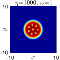
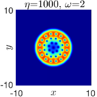
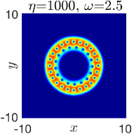
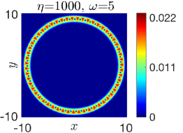
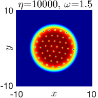
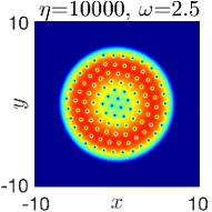
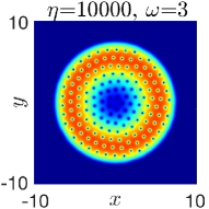
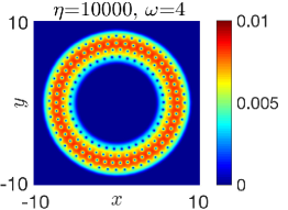
Figure 9: Exemple 6.7. Corresponding contour plots of the density function $|\phi_{g}(\mathbf{x})|^{2}$ of Table 1.

Example 6.8.

The choice of the initial data also affects the final converged stationary states. Since all the algorithms we discussed are local minimisation algorithms, inappropriate initial guess might lead to local minimum. To illustrate this claim, we take $\varepsilon=10^{-14}$, $V(\mathbf{x})=\frac{|\mathbf{x}|^{2}}{2}$, $\eta=500$ and compute the ground states of the rotating GPE for different $\omega$ and 10 types of frequently used initial data

$$(a)\ \phi_{a}(\mathbf{x})=\frac{1}{\sqrt{\pi}}e^{-(x^{2}+y^{2})/2},\qquad(b)\ \phi_{b}(\mathbf{x})=(x+iy)\phi_{a}(\mathbf{x}),\qquad(\bar{b})\ \phi_{\bar{b}}(\mathbf{x})=\bar{\phi}_{b}(\mathbf{x}),$$ (6.38)

$$(c)\ \phi_{c}=\frac{(\phi_{a}(\mathbf{x})+\phi_{b}(\mathbf{x}))/2}{\|(\phi_{a}(\mathbf{x})+\phi_{b}(\mathbf{x}))/2\|},\qquad\qquad(d)\ \phi_{d}=\frac{(1-\omega)\phi_{a}(\mathbf{x})+\omega\phi_{b}(\mathbf{x})}{\|(1-\omega)\phi_{a}(\mathbf{x})+\omega\phi_{b}(\mathbf{x})\|},$$ (6.39)

$$(e)\ \phi_{e}=\frac{\omega\phi_{a}(\mathbf{x})+(1-\omega)\phi_{b}(\mathbf{x})}{\omega\phi_{a}(\mathbf{x})+(1-\omega)\phi_{b}(\mathbf{x})\|},\qquad(\bar{c})\ \phi_{\bar{c}}(\mathbf{x})=\bar{\phi}_{c}(\mathbf{x}),\qquad(\bar{d})\ \phi_{\bar{d}}(\mathbf{x})=\bar{\phi}_{d}(\mathbf{x}),$$ (6.40)

$$(\bar{e})\ \phi_{\bar{e}}(\mathbf{x})=\bar{\phi}_{e}(\mathbf{x}),\qquad\qquad\qquad\qquad(f)\ {\rm Thomas\ Fermi\ approximation}\;\eqref{TF_App}.$$ (6.41)

Another approach to prepare some initial data is as follows: we first consider one of the above initial guess (a)-(f), next compute the ground state on a coarse spatial grid, say with a number of grid points $M_{p}\times M_{p}$ (with $M_{p}=2^{p}$), and then denote the corresponding stationary state by $\phi_{g}^{p}$. We next subdivide the grid with $M_{p+1}\times M_{p+1}$ points, interpolate $\phi_{g}^{p}$ on the refined grid $M_{p+1}\times M_{p+1}$ to get a new initial data and launch the algorithm at level $p+1$, and so on until the finest grid with $M\times M$ points where the converged solution is still denoted by $\phi_{g}$. Similarly to [44], this multigrid technique is applied here with the coarsest grid based with $M_{6}=2^{6}$ and ends with the finest grid $M=2^{9}$. We use the tolerance parameters $\varepsilon=10^{-14}$ for $M=2^{9}$, and $\varepsilon=10^{-12}$ for $p=6,7,8$.

Tables 2 and 3 list the energies obtained by PCG_C via the fixed and multigrid approaches, respectively, for different initial data and $\omega$. The stationary states $\phi_{g}(\mathbf{x})$ with lowest energies are marked by underlines and the corresponding CPU times are listed in the same Table. Moreover, Fig. 10 shows the contour plots $|\phi_{g}(\mathbf{x})|^{2}$ of the converged solution with lowest energy obtained by the multigrid approach. Now, let us denote by $E^{p}_{n}\mathrel{\mathop{\mathchar 58\relax}}=E(\phi_{n}^{p})$ the evaluated energy at step $n$ for a discretization level $p=6,7,8$, and let $E_{g}=E(\phi_{g})$ the energy for the converged stationary state for the finest grid. Then, we represent on Fig. 11 the evolution of $\log_{10}(|E^{p}_{n}-E_{g}|)$ vs. the CPU time for a rotating velocity $\omega=0.95$. For comparison, we also show the corresponding evolution obtained by the fixed grid approach. The contour plots of $|\phi^{p}_{g}(\mathbf{x})|^{2}$ obtained for each intermediate coarse grid for $p=6,7,8$, and the initial guess are also reported.

From these Tables and Figures, we can see that: (i) Usually, the PCG_C algorithm with an initial data of type ($d$) or ($\bar{d}$) converges to the stationary state of lowest energy; (ii) The multigrid approach is more robust than the fixed grid approach in terms of CPU time and possibility to obtain a stationary state with lower energy.

Table 2: Exemple 6.8. Fixed grid approach (with $M=2^{9}$): converged energies and the CPU times (seconds) for the solution with lowest energy (which is underlined).

  $\omega$ (a) (b) (b2) (c) (c2) (d) (d2) (e) (e2) (f) CPU 0.5 8.5118 8.2606 9.2606 8.0246 8.0197 8.0246 $\underline{8.0197}$ 8.0246 8.0197 8.0246 176.0 0.6 8.5118 8.1606 9.3606 7.5845 7.5910 7.5845 $\underline{7.5845}$ 7.5845 7.5910 7.5845 310.7 0.7 8.5118 8.0606 9.4606 6.9754 $\underline{6.9731}$ 6.9792 6.9754 6.9754 6.9792 6.9767 542.4 0.8 8.5118 7.9606 9.5606 6.1016 $\underline{6.0997}$ 6.1031 6.1031 6.1040 6.1019 6.1016 417.0 0.9 8.5118 7.8606 9.6606 4.7777 4.7777 4.7777 $\underline{4.7777}$ 4.7777 4.7777 4.7777 1051.1 0.95 8.5118 7.8106 9.7106 3.7414 3.7414 $\underline{3.7414}$ 3.7414 3.7414 3.7414 3.7414 3280.5  

Table 3: Exemple 6.8. Multigrid approach (starting from the coarsest level $p=6$ to the finest level $p=9$): converged energies and the CPU times (seconds) for the solution with lowest energy (underline).

  $\omega$ (a) (b) (b2) (c) (c2) (d) (d2) (e) (e2) (f) CPU 0.5 8.0246 8.0197 8.0197 8.0197 8.0197 8.0197 $\underline{8.0197}$ 8.0197 8.0197 8.0257 29.5 0.6 7.5845 7.5845 7.5910 7.5845 7.5910 7.5890 $\underline{7.5845}$ 7.5845 7.5910 7.5845 32.3 0.7 6.9767 $\underline{6.9726}$ 6.9792 6.9754 6.9731 6.9731 6.9731 6.9757 6.9731 6.9731 53.3 0.8 6.1019 6.1031 6.1019 $\underline{6.0997}$ 6.1016 6.1016 6.1016 6.1019 6.1016 6.0997 75.2 0.9 4.7777 4.7777 4.7777 4.7777 4.7777 $\underline{4.7777}$ 4.7777 4.7777 4.7777 4.7777 238.1 0.95 3.7414 3.7414 3.7414 3.7414 3.7414 $\underline{3.7414}$ 3.7414 3.7414 3.7414 3.7414 621.9  

  

  

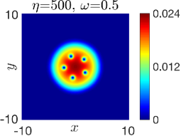
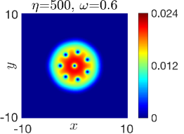
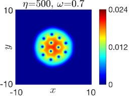
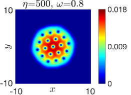
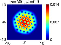
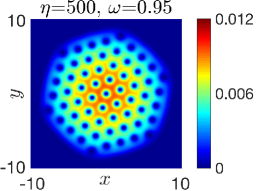
Figure 10: Contour plots of $|\phi_{g}(\mathbf{x})|^{2}$ corresponding to the lowest energy levels in Table 3.

 

       

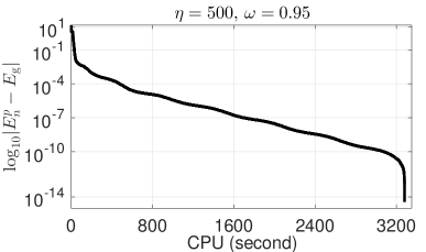
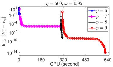
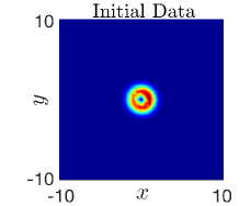
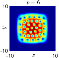
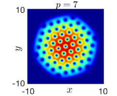
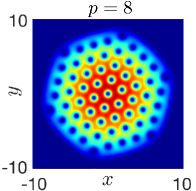
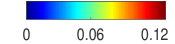
Figure 11: Exemple 6.8. Energy error $\log_{10}(|E^{p}_{n}-E_{g}|)$ vs. the accumulated CPU time for $\omega=0.95$ with initial data (d) in Table 2 ($p=9$, upper left) and respectively Table 3 (upper right) as well as the stationary state obtained at each intermediate level (lower, $p=6,7,8$)

6.3 Numerical results in 3D

Example 6.9.

Here, we apply the PCG_C algorithm to compute some realistic 3D challenging problems. To this end, $V(\mathbf{x})$ is chosen as the harmonic plus quartic potential (6.35), with $\gamma_{x}=\gamma_{y}=1$, $\gamma_{z}=3$, $\alpha=1.4$ and $\kappa=0.3.$ The computational domain is $\mathcal{D}=[-8,8]^{3}$ and the mesh size is: $h=\frac{1}{8}$. We test four cases: (i) $\eta=100$, $\omega=1.4$; (ii) $\eta=100$, $\omega=1.8$; (iii) $\eta=5000$ and $\omega=3$; (iv) $\eta=10000$ and $\omega=3$. The initial guess is always taken as the Thomas-Fermi initial data and the multigrid algorithm is used. Fig. 12 shows the isosurface $|\phi_{g}(\mathbf{x})|^{2}=10^{-3}$ and the surface plot of $|\phi_{g}(x,y,z=0)|^{2}$ for the four cases. The CPU times for these four cases are respectively 2256 s, 1403 s, 11694 s and 21971 s.

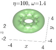
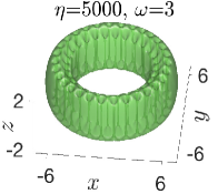
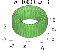
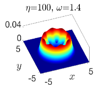
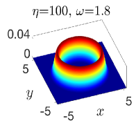
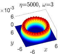
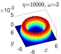
Figure 12: Exemple 6.9. Isosurface $|\phi_{g}(\mathbf{x})|^{2}=10^{-3}$ (upper) and surface plot of $|\phi_{g}(x,y,z=0)|^{2}$ (lower) in example 6.9. The CPU cost for these four cases are respectively 2256 (s), 1403 (s), 11694 (s) and 21971 (s).

7 Conclusion

We have introduced a new preconditioned nonlinear conjugate gradient algorithm to compute the stationary states of the GPE with fast rotation and large nonlinearities that arise in the modeling of Bose-Einstein Condensates. The method, which is simple to implement, appears robust and accurate. In addition, it is far more efficient than standard approaches as shown through numerical examples in 1D, 2D and 3D. Furthermore, a simple multigrid approach can still accelerates the performance of the method and leads to a gain of robustness thanks to the initial data. The extension to much more general systems of GPEs is direct and offers an interesting tool for solving highly nonlinear 3D GPEs, even for very large rotations.

References

- [1] J.R. Abo-Shaeer, C. Raman, J.M. Vogels, and W. Ketterle. Observation of vortex lattices in Bose-Einstein condensates. Science, 292(5516):476–479, APR 20 2001.
- [2] P-A Absil, R. Mahony, and R. Sepulchre. Optimization Algorithms on Matrix Manifolds. Princeton University Press, 2009.
- [3] S.K. Adhikari. Numerical solution of the two-dimensional Gross-Pitaevskii equation for trapped interacting atoms. Physics Letters A, 265(1-2):91–96, JAN 17 2000.
- [4] M.H. Anderson, J.R. Ensher, M.R. Matthews, C.E. Wieman, and E.A. Cornell. Observation of Bose-Einstein condensation in a dilute atomic vapor. Science, 269(5221):198–201, JUL 14 1995.
- [5] X. Antoine, W. Bao, and C. Besse. Computational methods for the dynamics of the nonlinear Schrödinger/Gross-Pitaevskii equations. Computer Physics Communications, 184(12):2621–2633, 2013.
- [6] X. Antoine and R. Duboscq. GPELab, a Matlab toolbox to solve Gross-Pitaevskii equations I: Computation of stationary solutions. Computer Physics Communications, 185(11):2969–2991, 2014.
- [7] X. Antoine and R. Duboscq. Robust and efficient preconditioned Krylov spectral solvers for computing the ground states of fast rotating and strongly interacting Bose-Einstein condensates. Journal of Computational Physics, 258:509–523, 2014.
- [8] X. Antoine and R. Duboscq. GPELab, a Matlab toolbox to solve Gross-Pitaevskii equations II: Dynamics and stochastic simulations. Computer Physics Communications, 193:95–117, 2015.
- [9] X. Antoine and R. Duboscq. Modeling and Computation of Bose-Einstein Condensates: Stationary States, Nucleation, Dynamics, Stochasticity. In Besse, C and Garreau, JC, editor, Nonlinear Optical and Atomic Systems: at the Interface of Physics and Mathematics, volume 2146 of Lecture Notes in Mathematics, pages 49–145. 2015.
- [10] Z. Bai, J. Demmel, J. Dongarra, A. Ruhe, and H. van der Vorst. Templates for the solution of algebraic eigenvalue problems: a practical guide. SIAM, 2000.
- [11] W. Bao. Ground states and dynamics of multi-component Bose-Einstein condensates. Multiscale Modeling and Simulation: A SIAM Interdisciplinary Journal, 2(2):210–236, 2004.
- [12] W. Bao and Y. Cai. Ground states of two-component Bose-Einstein condensates with an internal atomic Josephson junction. East Asian Journal on Applied Mathematics, 1:49–81, 2011.
- [13] W. Bao and Y. Cai. Mathematical theory and numerical methods for Bose-Einstein condensation. Kinetic and Related Models, 6(1):1–135, MAR 2013.
- [14] W. Bao, Y. Cai, and H. Wang. Efficient numerical methods for computing ground states and dynamics of dipolar Bose-Einstein condensates. Journal of Computational Physics, 229(20):7874–7892, 2010.
- [15] W. Bao and Q. Du. Computing the ground state solution of Bose-Einstein condensates by a normalized gradient flow. SIAM Journal on Scientific Computing, 25(5):1674–1697, 2004.
- [16] W. Bao, S. Jiang, Q. Tang, and Y. Zhang. Computing the ground state and dynamics of the nonlinear Schrödinger equation with nonlocal interactions via the nonuniform FFT. Journal of Computational Physics, 296:72–89, 2015.
- [17] W. Bao and W. Tang. Ground-state solution of Bose-Einstein condensate by directly minimizing the energy functional. Journal of Computational Physics, 187(1):230–254, MAY 1 2003.
- [18] R. Barrett, M. Berry, T. Chan, J. Demmel, J. Donato, J. Dongarra, V. Eijkhout, R. Pozo, C. Romine, and H. Van der Vorst. Templates for the solution of linear systems: building blocks for iterative methods. SIAM, 1994.
- [19] D. Baye and J.M. Sparenberg. Resolution of the Gross-Pitaevskii equation with the imaginary-time method on a Lagrange mesh. Physical Review E, 82(5), Nov 1 2010.
- [20] C.C. Bradley, C.A. Sackett, J.J. Tollett, and R.G. Hulet. Evidence of Bose-Einstein condensation in an atomic gas with attractive interactions. Physical Review Letters, 75(9):1687–1690, AUG 28 1995.
- [21] V. Bretin, S. Stock, Y. Seurin, and J. Dalibard. Fast rotation of a Bose-Einstein condensate. Physical Review Letters, 92(5), FEB 6 2004.
- [22] T. Byrnes, K. Wen, and Y. Yamamoto. Macroscopic quantum computation using Bose-Einstein condensates. Physical Review A, 85(4), 2012.
- [23] M. Caliari, A. Ostermann, S. Rainer, and M. Thalhammer. A minimisation approach for computing the ground state of Gross-Pitaevskii systems. Journal of Computational Physics, 228(2):349–360, FEB 1 2009.
- [24] E. Cances, M. Defranceschi, W. Kutzelnigg, C. Le Bris, and Y. Maday. Computational quantum chemistry: a primer. Handbook of numerical analysis, 10:3–270, 2003.
- [25] M.M. Cerimele, M.L. Chiofalo, F. Pistella, S. Succi, and M.P. Tosi. Numerical solution of the Gross-Pitaevskii equation using an explicit finite-difference scheme: An application to trapped Bose-Einstein condensates. Physical Review E, 62(1):1382–1389, JUL 2000.
- [26] M.L. Chiofalo, S. Succi, and M.P. Tosi. Ground state of trapped interacting Bose-Einstein condensates by an explicit imaginary-time algorithm. Physical Review E, 62(5):7438–7444, NOV 2000.
- [27] F. Dalfovo, S. Giorgini, L.P. Pitaevskii, and S. Stringari. Theory of Bose-Einstein condensation in trapped gases. Review of Modern Physics, 71(3):463–512, APR 1999.
- [28] I. Danaila and F. Hecht. A finite element method with mesh adaptivity for computing vortex states in fast-rotating Bose-Einstein condensates. Journal of Computational Physics, 229(19):6946–6960, SEP 20 2010.
- [29] I. Danaila and P. Kazemi. A new Sobolev gradient method for direct minimization of the Gross-Pitaevskii energy with rotation. SIAM J. Sci. Comput., 32(5):2447–2467, 2010.
- [30] K.B. David, M.O. Mewes, M.R. Andrews, N.J. Vandruten, D.S. Durfee, D.M. Kurn, and W. Ketterle. Bose-Einstein Condensation in gas of sodium atoms. Physical Review Letters, 75(22):3969–3973, NOV 27 1995.
- [31] C.M. Dion and E. Cances. Ground state of the time-independent Gross-Pitaevskii equation. Computer Physics Communications, 177(10):787–798, NOV 15 2007.
- [32] A. Edelman, T. A Arias, and S.T. Smith. The geometry of algorithms with orthogonality constraints. SIAM Journal on Matrix Analysis and Applications, 20(2):303–353, 1998.
- [33] A.V. Knyazev. Toward the optimal preconditioned eigensolver: locally optimal block preconditioned conjugate gradient method. SIAM Journal on Scientific Computing, 23(2):517–541, 2001.
- [34] K.W. Madison, F. Chevy, V. Bretin, and J. Dalibard. Stationary states of a rotating Bose-Einstein condensate: Routes to vortex nucleation. Physical Review Letters, 86(20):4443–4446, MAY 14 2001.
- [35] K.W. Madison, F. Chevy, W. Wohlleben, and J. Dalibard. Vortex formation in a stirred Bose-Einstein condensate. Physical Review Letters, 84(5):806–809, JAN 31 2000.
- [36] M.R. Matthews, B.P. Anderson, P.C. Haljan, D.S. Hall, C.E. Wieman, and E.A. Cornell. Vortices in a Bose-Einstein condensate. Physical Review Letters, 83(13):2498–2501, SEP 27 1999.
- [37] M.C. Payne, M.P. Teter, D.C. Allan, T.A. Arias, and J.D. Joannopoulos. Iterative minimization techniques for ab initio total-energy calculations: molecular dynamics and conjugate gradients. Reviews of Modern Physics, 64(4):1045–1097, 1992.
- [38] C. Raman, J.R. Abo-Shaeer, J.M. Vogels, K. Xu, and W. Ketterle. Vortex nucleation in a stirred Bose-Einstein condensate. Physical Review Letters, 87(21), NOV 19 2001.
- [39] Y. Saad. Iterative Methods for Sparse Linear Systems. SIAM, 2nd edition, 2003.
- [40] Y. Saad. Numerical Methods for Large Eigenvalue Problems. SIAM, 2011.
- [41] Y. Saad, J.R. Chelikowsky, and S.M. Shontz. Numerical methods for electronic structure calculations of materials. SIAM Review, 52(1):3–54, 2010.
- [42] M.P. Teter, M.C. Payne, and D.C. Allan. Solution of Schrödinger’s equation for large systems. Phys. Rev. B, 40:12255–12263, 1989.
- [43] Y.-S. Wang, B.-W. Jeng, and C.-S. Chien. A two-parameter continuation method for rotating two-component Bose-Einstein condensates in optical lattices. Communications in Computational Physics, 13:442–460, 2013.
- [44] X. Wu, Z. Wen, and W. Bao. A regularized Newton method for computing ground states of Bose-Einstein condensates. arXiv:1504.02891, 2015.
- [45] C. Yuce and Z. Oztas. Off-axis vortex in a rotating dipolar Bose-Einstein condensate. Journal of Physics B-Atomic Molecular and Optical Physics, 43(13), JUL 14 2010.
- [46] R. Zeng and Y. Zhang. Efficiently computing vortex lattices in rapid rotating Bose-Einstein condensates. Computer Physics Communications, 180(6):854–860, JUN 2009.
- [47] Y. Zhou, J.R. Chelikowsky, X. Gao, and A. Zhou. On the preconditioning function used in planewave dft calculations and its generalization. Communications in Computational Physics, 18(1):167–179, 2015.