Swimming by switching

Abstract

In this paper we investigate different strategies to overcome the scallop theorem. We will show how to obtain a net motion exploiting the fluid’s type change during a periodic deformation. We are interested in two different models: in the first one that change is linked to the magnitude of the opening and closing velocity. Instead, in the second one it is related to the sign of the above velocity. An interesting feature of the latter model is the introduction of a delay-switching rule through a thermostat. We remark that the latter is fundamental in order to get both forward and backward motion.

1 Introduction

The study of locomotion strategies in fluids is attracting increasing interest in recent literature, especially for its connection with the realization of artificial devices that can self-propel in fluids. Theories of swimming generally utilize either low Reynolds number approximation, or the assumption of inviscid ideal fluid dynamics (high Reynolds number). These two different regimes are also distinct in terms of the mechanism of locomotion Childress81; Lighthill75.
In this paper we focus on swimmers immersed in these two kind of fluids which produce a linear dynamics. In particular we study the system describing the motion of a scallop for which it is well known AlougesDeSimone08; GeneralizedScallop; Purcell77 that the scallop theorem/paradox holds. This means that it is not capable to achieve any net motion performing cyclical shape changes, either in a viscous or in an inviscid fluid. Some authors tried to overcome this paradox changing the geometry of the swimmer, for example adding a degree of freedom, introducing the Purcell swimmer Purcell77, or the three sphere swimmer Goldstein. Others, instead, supposed the scallop immersed in a non Newtonian fluid, in which the viscosity is not constant, ending up with a non reversible dynamics Pseudoelastic; Nature. Inspired by this last approach, our aim is to propose some strategies which maintain the swimmer geometry and exploit instead a change in the dynamics. The idea is based on switching dynamics depending on the angular velocity of opening and closing of the scallop’s valves. More precisely we analyze two cases: in the first one we suppose that if the modulus of the angular velocity is high, the fluid regime can be approximated by the ideal one, instead if this modulus is low the fluid can be considered as completely viscous. These assumptions are realistic since the Reynolds number changes depending on the characteristic velocity of the swimmer. In the second case we assume that the fluid reacts in a different way between the opening and closing of the valves: it facilitates the opening, so that it can be considered an ideal fluid, and resists the closing, like a viscous fluid. These last approximations model a fluid in which the viscosity changes with the sign of the angular velocity. More precisely we use two constant viscosities: one high (resp. one very small) if the angular velocity is negative (resp. positive). Moreover inspired by Nature, where the scallop’s opening and closing is actuated by an external magnetic field, in this last case we also introduce an hysteresis mechanism through a thermostat, see Fig LABEL:Fig00 (see Visintin for mathematical models for hysteresis), to model a delay in the change of fluid’s regime. In both cases we assume to be able to prescribe the angular velocity, using it as a control parameter and we prove that the system is controllable, i.e. the scallop is able to move both forward and backward using cyclical deformations. Furthermore we prove also that it is always possible to move between two fixed points, starting and ending with two prescribed angles.
In the last part of the paper we show also some numerical examples to support our theoretical predictions.

The plan of the paper is the following. In Section 2 we present the swimmer model and derive its equation of motion both in the viscous and in the ideal approximation, proving the scallop theorem. Section 3 is devoted to the introduction of the switching strategies which lead to the controllability of the scallop system. Finally in Section LABEL:sec:4 we present some numerical simulations showing different kind of controls that can be used.

2 The Scallop swimmer

In this section we are interested in analyzing the motion of an articulated rigid body immersed in a fluid that changes its configuration. In order to determine completely its state we need the position of its center of mass and its orientation. Their temporal evolution is obtained solving the Newton’s equations coupled with the Navier-Stokes equations relative to the surrounding fluid. We will face this problem considering the body as immersed in two kinds of different fluids: one viscous at low Reynolds number in which we neglect the effects of inertia, and another one ideal inviscid and irrotational, in which we neglect the viscous forces in the Navier-Stokes equations. First of all we recall that in both cases a swimmer that tries to moves like a scallop, opening and closing periodically its valves, does not move at the end of a cycle. This situation is well known as scallop theorem (or paradox) AlougesDeSimone08; Purcell77.
In what follows we will consider a planar body composed by two rigid valves of elliptical shape, joined in order that they can be opened and closed. Moreover this body is constrained to move along one of the cartesian axes (the $\vec{e}_{x}$-axis) and is symmetric with respect to it. Finally we will neglect the interaction between the two valves. The configuration of the system is easily described by the position $x$ of the juncture point along the $\vec{e}_{x}$-axis and by the angle $\theta$ that each valve forms with the axis

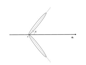
Figure 1: The scallop configuration

The possible translation of the system is determined by the consecutive opening and closing of the valves. Our aim is to determine the net translation of the body, given the function of time describing the angular velocity $\dot{\theta}$.

2.1 Viscous fluid

Here we focus on the case in which the scallop is immersed in a viscous fluid. In this regime the viscous forces dominates the inertial ones that can be neglected, so the equations governing the dynamics of the fluid are the Stokes ones:

$$\Delta v-\nabla p=0$$

together with the incompressibility condition $\textrm{div}\ v=0$. Let us consider that the ellipses have major axis $2a$ and minor axis $2b$ with $b<<a$, moreover let us suppose that $\theta\in(0,\frac{\pi}{2})$ so that it remains acute. One of the main difficulties in computing explicitly the equation of motion is the complexity of the hydrodynamic forces exerted by the fluid on the swimmer as a reaction to its shape changes. Since in our assumptions the minor axis of the ellipse is very small with respect to the major one, i.e. $b<<a$, we can consider the swimmer as one-dimensional, composed essentially by two links of length $2a$ (see Fig 1). In the case of slender swimmers, Resistive Force Theory (RFT) GrayHancock55 provides a simple and concise way to compute a local approximation of such forces, and it has been successfully used in several recent studies, see for example BeckerKoehler03; FriedrichRiedel-Kruse10. From now on we use this approach as well, in order to obtain the forces acting on the swimmer, neglecting the interaction between the valves. Since the scallop is immersed in a viscous fluid the inertial forces are negligible with respect to the viscous ones, therefore the dynamics of the swimmer follows from Newton laws in which inertia vanishes:

$$\vec{F}=0$$ (1)

where $\vec{F}$ is the total force exerted on the swimmer by the fluid. As already said we want to couple the fluid and the swimmer, using the local drag approximation of Resistive Force Theory. We denote by $s$ the arc length coordinate on the $i$-th link ($0\leq s\leq 2a$) measured from the juncture point and by $\vec{v}_{i}(s)$ the velocity of the corresponding point. We also introduce the unit vectors $\vec{e}_{1}=\left(\begin{array}[]{cc}\cos(\theta)\\ \sin(\theta)\\ \end{array}\right)$, $\vec{e}_{1}^{\bot}=\left(\begin{array}[]{cc}-\sin(\theta)\\ \cos(\theta)\\ \end{array}\right)$, and $\vec{e}_{2}=\left(\begin{array}[]{cc}\cos(\theta)\\ -\sin(\theta)\\ \end{array}\right)$, $\vec{e}_{2}^{\bot}=\left(\begin{array}[]{cc}-\sin(\theta)\\ -\cos(\theta)\\ \end{array}\right)$ in the directions parallel and perpendicular to each link and write the position of the point at arc length $s$ as $\vec{x}_{i}(s)=\left(\begin{array}[]{c}x\\ 0\end{array}\right)+s\vec{e}_{i}$ where x is the coordinate of the joint between the two valves. By differentiation, we obtain,

$$\vec{v}_{i}(s)=\left(\begin{array}[]{c}\dot{x}\\ 0\end{array}\right)+s\dot{\theta}_{i}\vec{e}_{i}^{\bot}\,.$$ (2)

The density of the force $\vec{f}_{i}$ acting on the $i$-th segment is assumed to depend linearly on the velocity. It is defined by

$$\vec{f}_{i}(s):=-\xi\left(\vec{v}_{i}(s)\cdot\vec{e}_{i}\right)\vec{e}_{i}-\eta\left(\vec{v}_{i}(s)\cdot\vec{e}_{i}^{\bot}\right)\vec{e}_{i}^{\bot},$$ (3)

where $\xi$ and $\eta$ are respectively the drag coefficients in the directions of $\vec{e}_{i}$ and $\vec{e}_{i}^{\bot}$ measured in $N\,s\,m^{-2}$. We thus obtain

$$\vec{F}=\int_{0}^{2a}\vec{f}_{1}(s)\,ds+\int_{0}^{2a}\vec{f}_{2}(s)\,ds=0$$ (4)

Using (2) and (3) and since we are neglecting inertia we have

$$\begin{cases}F_{x}=-4a\xi\dot{x}\cos^{2}(\theta)-4a\eta\dot{x}\sin^{2}(\theta)+4a^{2}\eta\dot{\theta}\sin(\theta)=0\\ F_{y}=0\end{cases}$$ (5)

Observe that $F_{y}$ vanishes since the scallop is symmetric with respect to the $\vec{e}_{x}$ axis. From (5) is now easy to determine the evolution of $x$

$$\dot{x}=V_{1}(\theta)\dot{\theta}=\frac{a\eta\sin(\theta)}{\xi\cos^{2}(\theta)+\eta\sin^{2}(\theta)}\dot{\theta}$$ (6)

2.2 Ideal Fluid

While in the previous subsection we faced the problem of the self-propulsion of the scallop immersed in a viscous fluid, here we focus on the case in which it is immersed in an ideal inviscid and irrotational fluid. Let us make the same assumptions on the parameters $a$ and $b$ that have been done in the previous section, moreover let us denote by $\Omega$ the region of the plane occupied by the swimmer in a reference configuration.

Assigning $(x,\theta)$ as functions of time let us call

$$f^{(x,\theta)}: \Omega\to\mathbb{R}^{2}$$

$$\zeta\mapsto f^{(x,\theta)}(\zeta)$$

the function which maps each point of the swimmer $\zeta\in\Omega$ in $f^{(x,\theta)}(\zeta)$ that is its position in the plane at time $t$. Supposing that $\theta$ can be assigned and that there are not other external forces, our aim is to find equations that describe the motion of $x$. To this end we call $v$ the velocity of the fluid, its motion is given by the Euler equations for ideal fluids

$$v_{t}+v\cdot\nabla v=-\nabla p$$ (7)

with the incompressibility condition $\textrm{div}\ v=0$. Moreover we impose a Neumann boundary condition, that is that the normal component of the velocity of the fluid has to be equal to the normal component of the velocity of the body.

$$\Bigl{\langle}v(f^{(x,\theta)})-\bigl{(}\frac{\partial f^{(x,\theta)}}{\partial x}\dot{x}+\frac{\partial f^{(x,\theta)}}{\partial\theta}\dot{\theta}\bigr{)},n^{(x,\theta)}\Bigr{\rangle}=0$$

where $\Bigl{\langle}\cdot\Bigr{\rangle}$ denotes the scalar product, $n^{(x,\theta)}$ is the external normal to the set $f^{(x,\theta)}(\Omega)$. To find the evolution of $x$ we should solve the Lagrange equation

$$\frac{d}{dt}\frac{\partial T^{b}}{\partial\dot{x}}=\frac{\partial T^{b}}{\partial x}+F$$ (8)

where $T^{b}$ is the kinetic energy of the body and $F$ the external pressure force acting on the boundary of the swimmer. As already done in Bressan07; MasonBurdick99; MunnierChambrion10 this force $F$ can be reinterpreted as a kinetic term, precisely thanks to the fact that we are in an ideal fluid. Therefore the system body + fluid is geodetic with Lagrangian given by the sum of the kinetic energy of the body ($T^{b}$) and the one of the fluid ($T^{f}$):

$$T^{tot}=T^{b}+T^{f}$$

The kinetic energy of the body is the sum of the kinetic energy of the two ellipses, that reads

$$T^{b}=m\bigl{(}\dot{x}^{2}+a^{2}\dot{\theta}^{2}-2a\dot{x}\dot{\theta}\sin\theta\bigr{)}+I\dot{\theta}^{2}$$ (9)

Since we are dealing with an ideal fluid and thus inertial forces dominates over the viscous ones, in order to derive the kinetic energy of the fluid we will make use of the concept of added mass. In fluid mechanics, added mass or virtual mass is the inertia added to a system because an accelerating or decelerating body must move (or deflect) some volume of surrounding fluid as it moves through it. Added mass is a common issue because the object and surrounding fluid cannot occupy the same physical space simultaneously Bessel28. For simplicity this can be modeled as some volume of fluid moving with the object, though in reality ”all” the fluid will be accelerated, to various degrees.
Therefore the kinetic energy of the fluid will be given by the sum of the kinetic energy of the added masses of the two ellipses.

$$T^{f}=\frac{1}{2}\vec{v}_{1}^{T}\vec{M}_{1_{add}}\vec{v}_{1}+\frac{1}{2}\vec{v}_{2}^{T}\vec{M}_{2_{add}}\vec{v}_{2}$$ (10)

where $\vec{M}_{i_{add}}$ are the added mass matrices relative to each ellipse which are diagonal, and $\vec{v}_{i}$ the velocities of their centre of mass, expressed in the frame solidal to each ellipse with axes parallel and perpendicular to the major axis. Finally we can compute the total kinetic energy of the coupled system body+ fluid that is

$$T^{tot} =m\bigl{(}\dot{x}^{2}+a^{2}\dot{\theta}^{2}-2a\dot{x}\dot{\theta}\sin\theta\bigr{)}+I\dot{\theta}^{2}+$$ (11)

$$+m_{11}\dot{x}^{2}\cos^{2}\theta+m_{22}\bigl{(}\dot{x}^{2}\sin^{2}\theta+a^{2}\dot{\theta}^{2}-2a\dot{x}\dot{\theta}\sin\theta\bigr{)}+$$

$$+m_{3}3\dot{\theta}^{2}$$

Following a procedure introduced by Alberto Bressan in Bressan07, in order to end up with a control system we perform a partial legendre transformation on the kinetic energy defining

$$p= \frac{\partial T^{tot}}{\partial\dot{x}}=$$

$$2\dot{x}\bigl{(}m+m_{11}\cos^{2}\theta+m_{22}\sin^{2}\theta\bigr{)}-2a\dot{\theta}\sin\theta(m+m_{22})$$

from which we derive

$$\dot{x}=\frac{p+2a\dot{\theta}\sin\theta(m+m_{22})}{2(m+m_{11}\cos^{2}\theta+m_{22}\sin^{2}\theta)}$$ (12)

There is a wide spread literature regarding the computation of added masses of planar contours moving in an ideal unlimited fluid. We will use in the rest of the paper the added mass coefficients for the ellipse computed in Marhydro: the added mass in the direction of the major axis is $m_{11}=\rho\pi b^{2}$, the one along the minor axis is $m_{22}=\rho\pi a^{2}$. Notice now that writing the Hamilton equation relative to $p$, and recalling (11)

$$\dot{p}=\frac{\partial T^{tot}}{\partial x}=0$$

thus, if we start with $p(0)=0$, $p$ remains null for all times and the evolution of $x$ becomes

$$\dot{x}=V_{2}(\theta)\dot{\theta}=\frac{a\sin\theta(m+\rho\pi a^{2})}{m+\rho\pi b^{2}\cos^{2}\theta+\rho\pi a^{2}\sin^{2}\theta}\dot{\theta}$$ (13)

Theorem 2.1 (Scallop Theorem)

Consider a swimmer dynamics of the type

$$\dot{x}=V(\theta)\dot{\theta}$$ (14)

Then for every $T$-periodic deformation (i.e. stroke) one has

$$\Delta x=\int_{0}^{T}\dot{x}(t)\,dt=0$$ (15)

that is, the final total translation is null

Proof

Define the primitive of $V$ by

$$F(\theta)=\int_{0}^{\theta}V(\sigma)\,d\sigma$$ (16)

Then using (14)

$$\Delta x =\int_{0}^{T}V(\theta(t))\dot{\theta}(t)\,dt=$$

$$\int_{0}^{T}\frac{d}{dt}F(\theta(t))\,dt=F(\theta(T))-F(\theta(0))=0$$

by the periodicity of $t\to\theta(t)$.∎

Note that the dynamics (6) and (13) are of the type (14), therefore the scallop theorem is valid either in the viscous and in the ideal case.

3 Controllability

In this section we will give two different strategies to overcome the scallop theorem, both based on a switching mechanism. In particular we produce some partial and global controllability results for this switching systems.

3.1 Partial controllability in $x$

We have previously seen that if our scallop is immersed either in an ideal fluid or in a viscous one, if it experiences periodical shape changes it is not able to move after one cycle. Here we would like to find a way to overcome this problem. The main idea is to be able to change the dynamics during one periodical stroke and see if in this way we obtain a net motion and in particular some controllability. In order to do this we have to introduce the Reynolds number, a number which characterizes the fluid regime. It arises from the adimesionalization of the Navier-Stokes equations and it is defined by

$$Re=\frac{VL\rho}{\eta}=\frac{VL}{\nu}$$ (17)

where $V$ is the characteristic velocity of the body immersed in the fluid, $L$ its characteristic length, $\rho$ the density of the fluid, $\eta$ its viscosity and $\nu=\frac{\eta}{\rho}$ is the kinematic viscosity. The Reynolds number quantifies the relative importance of inertial versus viscous effects.

3.1.1 $\boxed{\eta=\eta(|\dot{\theta}|)}$

Let us recall that if $v(t,x)$ is a solution of the Navier Stokes equations, the function $u(t,x)=v(ct,x)$, $c>0$ is still a solution of the Navier Stokes equations but with a different viscosity. Now assume that the absolute value of the speed $\dot{\theta}$ is very high, this means that rescaling the time of the solution of the Navier Stokes equations, we end up with a viscosity $\eta$ that is very small and therefore the Reynolds number is large. In this case the inertial forces dominates over the viscous ones, so we can consider the scallop immersed in an ideal fluid and thus use the dynamics (13). Then we suppose that at a certain point of the cycle the absolute value of the angular velocity is very small. In this case we have a solution of the Navier Stokes equations with a very high viscosity $\eta$. Thus we can suppose that the scallop is immersed in a Stokes fluid, since the viscous effects dominates the inertial ones and use the dynamics (6). This situation is well represented by a switching system in which the change of the dynamics is determined by the modulus of the angular velocity $\dot{\theta}$: if it is big (i.e $|\dot{\theta}|>M$ with $M>0$) we use the ideal approximation and the corresponding dynamics; if it is small (i.e $|\dot{\theta}|<M$ with $M>0$) we use instead the viscous approximation and the relative dynamics.The switching rule in Fig 2 should also consider what happens when $|\dot{\theta}|=M$. However in the sequel we are going to exhibit a function $\dot{\theta}$ which stays in $M$ or $-M$ for only a set of times of null measure.
Our aim is to prove that using this kind of switching we are able to have a net displacement, both forward or backward, using periodic continuous functions $\dot{\theta}$

According to what said before we can prescribe the angular velocity $\dot{\theta}$ and thus use it as a control function $u$. Therefore we write the system as a control system that is

$$\begin{cases}\dot{x}(t)=V_{w(t)}(\theta(t))u(t),\\ \dot{\theta}(t)=u(t)\\ w(t)=h[u](t)\\ x(0)=x_{0},\ \theta(0)=\theta_{0}\ \ w(0)=w_{0}\end{cases}$$

where $u$ is continuous and

$$h[u]=\begin{cases}2\quad\text{if $|u|>M$}\\ 1\quad\text{if $|u|<M$}\end{cases}$$

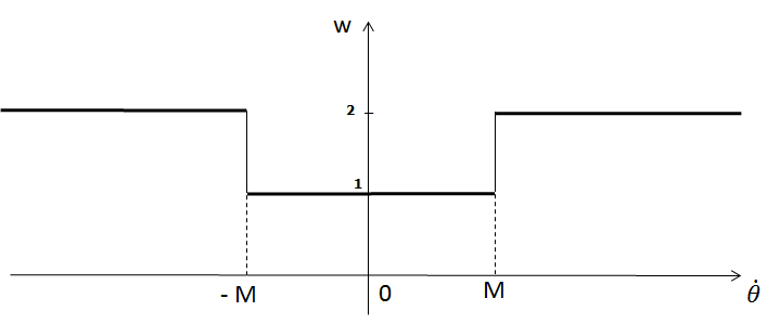
Figure 2: The rule of the classical switching

Moreover let us call $F_{i}$ the primitives of the functions $V_{i}$, for $i=1,2$. They are :

$$F_{1}=\frac{a\eta\arctan h(\sqrt{\frac{\eta-\xi}{\eta}}\cos\theta)}{\sqrt{\eta(\eta-\xi)}},$$

$$F_{2}=\frac{-a\sqrt{m+a^{2}\rho\pi}\arctan h(\frac{\sqrt{(a^{2}-b^{2})\rho\pi}\cos\theta}{\sqrt{m+a^{2}\rho\pi}})}{\sqrt{\rho\pi(a^{2}-b^{2})}}$$

Theorem 3.1

With the previous switching scheme we are able to overcome the Scallop paradox, thus to move both forward and backward. More precisely there are $r>0$ small enough (see remark LABEL:erre1), a final time $T>0$ and a continuous $T$-periodic control function $u(t)$, which make the system move between two fixed points along the $x$ axis, $x_{0}$ and $x_{f}\in]x_{0}-r,x_{0}+r[$, in the time $T$.