Flux-limited and classical viscosity solutions for regional control problems

Abstract

The aim of this paper is to compare two different approaches for regional control problems: the first one is the classical approach, using a standard notion of viscosity solutions, which is developed in a series of works by the three first authors. The second one is more recent and relies on ideas introduced by Monneau and the fourth author for problems set on networks in another series of works, in particular the notion of flux-limited solutions. After describing and even revisiting these two very different points of view in the simplest possible framework, we show how the results of the classical approach can be interpreted in terms of flux-limited solutions. In particular, we give much simpler proofs of three results: the comparison principle in the class of bounded flux-limited solutions of stationary multidimensional Hamilton-Jacobi equations and the identification of the maximal and minimal Ishii’s solutions with flux-limited solutions which were already proved by Monneau and the fourth author, and the identification of the corresponding vanishing viscosity limit, already obtained by Vinh Duc Nguyen and the fourth author.

Key-words: Optimal control, discontinuous dynamic, Bellman Equation, flux-limited solutions, viscosity solutions.
MSC: 49L20, 49L25, 35F21.

1 Introduction

Recently, a lot of works have been devoted to the study of deterministic control problems involving discontinuities and, more precisely, problems where the dynamics and running costs may be completely different in different parts of the domain. In fact, these problems can be of different natures: first, they may only deal with “simple” discontinuities of codimension $1$ like in [7], [9, 8], [16]; the first three authors provide in [2, 3] a systematic study of such problems and we describe these results below. Second, following Bressan & Hong [6], other results are concerned with problems in “stratified domains”, where the discontinuities can be of any codimension; we refer to [5] for a new and simpler approach of these problems, with new results. Third, they are problems set on networks for which the specified methods are required since such singular domains are not necessarily contained in $\mathbb{R}^{N}$; we refer to [1], [12], [15], [11], [10], [13] [14], for different approaches of such networks problems.

The aim of this article is to compare the different approaches used in these articles, and in particular the ones of [2, 3] and [11, 10]. Indeed, this link is only presented in the mono-dimensional setting in [11]; see also [10]. In order to provide the clearest possible picture, we consider the simplest possible case, namely the case of two half-spaces in $\mathbb{R}^{N}$, say $\Omega_{1}:=\{x=(x_{1},\cdots,x_{N});x_{N}>0\}$ and $\Omega_{2}:=\{x=(x_{1},\cdots,x_{N});x_{N}<0\}$ and we also choose below the most simple assumptions on either the control problem or the Hamilton-Jacobi Equations (controllability or coercivity). In the same line, we restrict ourselves to the case of stationary Hamilton-Jacobi equations, corresponding to infinite-time horizon control problems (with actualization factor $\lambda=1$).

The first key step, and this is one major difference in the above mentioned works, is to identify the questions we are interested in and/or the methods we are able to use. This is where the fact to be in $\mathbb{R}^{N}$ or on a network changes completely the point of view. In [2, 3], the key questions were the following. First, consider the equations

$$u+H_{1}(x,Du)=0\quad\hbox{in }\Omega_{1}\;,$$ (1.1)

$$u+H_{2}(x,Du)=0\quad\hbox{in }\Omega_{2}\;,$$ (1.2)

then the classical Ishii’s definition of viscosity solutions implies that we have “natural junction conditions” on $\mathcal{H}:=\overline{\Omega}_{1}\cap\overline{\Omega}_{2}=\left\{x\in\mathbb{R}^{N}\>:\>x_{N}=0\right\}$ which read

$$\min(u+H_{1}(x,Du),u+H_{2}(x,Du))\leq 0\quad\hbox{on }\mathcal{H}\;,$$ (1.3)

$$\max(u+H_{1}(x,Du),u+H_{2}(x,Du))\geq 0\quad\hbox{on }\mathcal{H}\;.$$ (1.4)

Indeed, if $H$ is the Hamiltonian defined by

$$H(x,u,p):=\left\{\begin{array}[]{ll}u+H_{1}(x,p)&\hbox{if $x\in\Omega_{1}$}\\ u+H_{2}(x,p)&\hbox{if $x\in\Omega_{2}$}\end{array}\right.$$

then the above inequalities are nothing but $H_{*}\leq 0$ and $H^{*}\geq 0$ on $\mathcal{H}$. Unfortunately, these junction conditions are not enough to ensure uniqueness and there may (and in general do) exist several Ishii’s discontinuous solutions.

The first question which is addressed in [2, 3] is to define properly a control problem where the dynamics and running cost are different in $\Omega_{1}$ and $\Omega_{2}$. The main problem concerns the controlled trajectories which may stay on $\mathcal{H}$: how to properly define them and do they lead to the junction conditions (1.3)-(1.4)? Then the next question is to identify the maximal and minimal solutions of (1.1)-(1.2)-(1.3)-(1.4) when $H_{1}$, $H_{2}$ are Hamiltonians of control problems (see Theorem 3.4 at the end of Section 3). A key remark on these results is that the use of differential inclusions methods leads on $\mathcal{H}$ to a mixing of the dynamics-costs of $\Omega_{1}$ and $\Omega_{2}$ and this is actually (depending on the type of mixing one allows) how the maximal and minimal solutions of (1.1)-(1.2)-(1.3)-(1.4) are defined. This approach (refered below as CVS $=$ classical viscosity solutions’ approach) is described in Section 3 with the main results.

In the network framework, the question of how to define the junction condition(s) becomes more central since the definition of classical Ishii’s definition of viscosity solutions is not straightforward in the general case. Such a difficulty is related to another important difference (which is not addressed at all in [2, 3]) which is the choice of the set of test-functions: while in $\mathbb{R}^{N}$, even with the discontinuities on $\mathcal{H}$, the choice of test-functions which are $C^{1}$ in $\mathbb{R}^{N}$ is natural, this choice makes no sense in the network framework where the “natural” set of test-functions is the set of functions which are $C^{1}$ on each branch and continuous at the junctions. Here, if test-functions are chosen to be continuous in $\mathbb{R}^{N}$, $C^{1}$ in $\Omega_{1}$ and $\Omega_{2}$ and to have a trace on $\mathcal{H}$ which is $C^{1}$ on $\mathcal{H}$ (allowing a jump on the $x_{N}$-derivative), the question is: what does this change in the [2, 3] picture?

In order to answer this question, we first describe the flux-limited solution approach (FL-approach in short) consisting in adding a junction condition $G$ on $\mathcal{H}$. It can be seen as being associated to a particular control problem on $\mathcal{H}$. This function $G$ is called the flux limiter in [11, 10]. Compared to [2, 3], this approach is more PDE-oriented: we give and comment the definition with test-functions which are just piecewise $C^{1}$. Even if it is rather natural from the control point of view, it turns out to be rather different from the classical Ishii’s definition.

For the FL-approach, we provide a simplified uniqueness proof for the associated Hamilton-Jacobi-Bellman Equations obtained in [10]. Instead of using the so-called vertex test function (which construction is difficult and lengthy), we simply use specific slopes identified in [11, 10] (see Lemma A.3 in Appendix) in order to construct a simple test function. Indeed, it is explained in [11, 10] that a function is a flux-limited solution if it satisfies the viscosity inequality on $\mathcal{H}$ only when tested with smooth functions whose derivatives at the junction coincide with those specific slopes. We do not need such a result about the reduction of test functions here but, guided by this idea, we give a simpler proof of the comparison principle. Finally we identify the value-function ($\mathbf{U}^{\mathrm{FL}}_{G}$) which is the unique solution of this problem associated to $G$.

The next question is the comparison of the two (apparently very different) approaches in the multi-dimensional setting: it turns out that, as in the mono-dimensional setting [11], the maximal ($\mathbf{U}^{+}$) and minimal ($\mathbf{U}^{-}$) solutions in the CVS-approach can be recovered by using the right “flux limiter” $G$ (or control problem) on $\mathcal{H}$: these flux limiters are respectively the Hamiltonians $H_{T}^{\rm reg}$ and $H_{T}$ identified in [2, 3]. We conclude that the FL-approach provides a completely different way (and with pure PDE methods) to address the questions solved in [2, 3]. Moreover, the choice of $G$ (in particular the case when there is no such a flux limiter) allows one to consider different control problems on $\mathcal{H}$ in a more general way than in [2, 3].

Last but not least, this clear understanding on the advantages and disadvantages of the two points of view for looking at the HJ problem with discontinuities, allows us to simplify the proof of the convergence of the vanishing viscosity approximation, a result already given in [13].

The article is organized as follows: in Section 2, we describe the FL-approach with the simplified comparison proof and the connection with the related control problem. Then in Section 3, we recall the CVS-approach; the two approaches are compared in Section 4. The convergence of the vanishing viscosity approximation closes the article (Section 5). The appendix contains technical results which are used in the paper.

2 Flux-limited solutions

2.1 Assumptions and definitions

We first describe the assumptions on the dynamic and running cost in each $\Omega_{i}\ (i=1,2)$ and on $\mathcal{H}$ since they are used to define the junction conditions. We recall that we use the simplest possible assumptions and we formulate the problem in the simplest possible way by assuming that the dynamics and running costs are defined in the whole space $\mathbb{R}^{N}$.

On $\Omega_{i}$, the sets of controls are denoted by $A_{i}$, the system is driven by a dynamic $b_{i}$ and the running cost is given by $l_{i}$. We use the index $i=0$ for $\mathcal{H}$. Our main assumptions are the following.

• For $i=0,1,2$, $A_{i}$ is a compact metric space and $b_{i}:\mathbb{R}^{N}\times A_{i}\rightarrow\mathbb{R}^{N}$ is a continuous bounded function, more precisely $|b_{i}(x,\alpha_{i})|\leq M_{b}$ for all $x\in\mathbb{R}^{N}$ and $\alpha_{i}\in A_{i}$, $i=0,1,2$. Moreover, there exists $L_{i}\in\mathbb{R}$ such that, for any $x,y\in\mathbb{R}^{N}$ and $\alpha_{i}\in A_{i}$

  $$|b_{i}(x,\alpha_{i})-b_{i}(y,\alpha_{i})|\leq L_{i}|x-y|\;.$$

• For $i=0,1,2$, the function $l_{i}:\mathbb{R}^{N}\times A_{i}\rightarrow\mathbb{R}^{N}$ is continuous and $|l_{i}(x,\alpha_{i})|\leq M_{l}$ for all $x\in\mathbb{R}^{N}$ and $\alpha_{i}\in A_{i}$, $i=1,2$.

The last assumption is a controlability assumption that we use only in $\Omega_{1}\cup\Omega_{2}$, and not on $\mathcal{H}$.

• For each $x\in\mathbb{R}^{N}$, the sets $\left\{(b_{i}(x,\alpha_{i}),l_{i}(x,\alpha_{i}))\>:\>\alpha_{i}\in A_{i}\right\}$, ($i=1,2$), are closed and convex. Moreover there is a $\delta>0$ such that for any $i=1,2$ and $x\in\mathbb{R}^{N}$,

  $$\overline{B(0,\delta)}\subset B_{i}(x):=\left\{b_{i}(x,\alpha_{i})\>:\>\alpha_{i}\in A_{i}\right\}.$$ (2.1)

We now define several Hamiltonians. For $x\in\overline{\Omega}_{1}$

$$H_{1}(x,p):=\sup_{\alpha_{1}\in A_{1}}\left\{-b_{1}(x,\alpha_{1})\cdot p-l_{1}(x,\alpha_{1})\right\}\,,$$ (2.2)

$$H_{1}^{-}(x,p):=\sup_{\alpha_{1}\in A_{1}\>:\>b_{1}(x,\alpha_{1})\cdot e_{N}\leq 0}\left\{-b_{1}(x,\alpha_{1})\cdot p-l_{1}(x,\alpha_{1})\right\}\,,$$ (2.3)

$$H_{1}^{+}(x,p):=\sup_{\alpha_{1}\in A_{1}\>:\>b_{1}(x,\alpha_{1})\cdot e_{N}>0}\left\{-b_{1}(x,\alpha_{1})\cdot p-l_{1}(x,\alpha_{1})\right\}\,,$$ (2.4)

and for $x\in\overline{\Omega}_{2}$

$$H_{2}(x,p):=\sup_{\alpha_{2}\in A_{2}}\left\{-b_{2}(x,\alpha_{2})\cdot p-l_{2}(x,\alpha_{2})\right\}\,,$$ (2.5)

$$H^{+}_{2}(x,p):=\sup_{\alpha_{2}\in A_{2}\>:\>b_{2}(x,\alpha_{2})\cdot e_{N}\geq 0}\left\{-b_{2}(x,\alpha_{2})\cdot p-l_{2}(x,\alpha_{2})\right\}\,,$$ (2.6)

$$H^{-}_{2}(x,p):=\sup_{\alpha_{2}\in A_{2}\>:\>b_{2}(x,\alpha_{2})\cdot e_{N}<0}\left\{-b_{2}(x,\alpha_{2})\cdot p-l_{2}(x,\alpha_{2})\right\}\,.$$ (2.7)

Finally, for the specific control problem on $\mathcal{H}$ we define for any $x\in\mathcal{H}$ and $p_{\mathcal{H}}\in\mathbb{R}^{N-1}$

$$G(x,p_{\mathcal{H}}):=\sup_{\alpha_{0}\in{\cal A}_{0}}\{-b_{0}(x,\alpha_{0})\cdot p_{\mathcal{H}}-l_{0}(x,\alpha_{0})\}\,.$$ (2.8)

In the sequel, the points of $\mathcal{H}$ are identified indifferently by $x^{\prime}\in\mathbb{R}^{N-1}$ or by $x=(x^{\prime},0)\in\mathbb{R}^{N}$. For the gradient variable we use the decomposition $p=(p_{\mathcal{H}},p_{N})$ where $p_{\mathcal{H}}\in\mathcal{H}=\mathbb{R}^{N-1}$ and $p_{N}\in\mathbb{R}$, and, when dealing with a function $u$, we also use the notation $D_{\mathcal{H}}u$ for the ${(N-1)}$ first components of the gradient, i.e.,

$$D_{\mathcal{H}}u:=(\frac{\partial u}{\partial x_{1}},\cdots,\frac{\partial u}{\partial x_{n-1}})\quad\hbox{and}\quad Du=\Big{(}D_{\mathcal{H}}u,\frac{\partial u}{\partial x_{N}}\Big{)}\,.$$

Note that, for the sake of consistency of notation, we also denote by $D_{\mathcal{H}}u$ the gradient of a function $u$ which is only defined on $\mathbb{R}^{N-1}$.

Let us remark that, thanks to assumptions [H0], [H1], the Hamiltonians $H_{i}$, $H_{i}^{\pm}$ ($i=1,2$) satisfy the following classical structure conditions: for any $R>0$, for any $x,y\in\mathbb{R}^{N}$ such that $|x|,|y|\leq R$, for any $p,q\in\mathbb{R}^{N}$ and for $i=1,2$

$$\begin{cases}|H_{i}(x,p)-H_{i}(x,q)|\leq M_{b}|p-q|\\ |H_{i}(x,p)-H_{i}(y,p)|\leq L_{i}|x-y|(1+|p|)+m_{i}^{R}(|x-y|)\;,\end{cases}$$ (2.9)

where $m_{i}^{R}$ is a (non-decreasing) modulus of continuity of the function $l_{i}$ on the compact set $\overline{B(0,R)}\times A_{i}$.

The assumptions on the function $G$ mimic the assumptions naturally satisfied by $H_{1},H_{2}$.

• The function $G:\mathcal{H}\times\mathbb{R}^{N-1}\rightarrow\mathbb{R}$ is continuous and satisfies: for any $x\in\mathcal{H}$, the function $p^{\prime}\mapsto G(x,p^{\prime}):\mathbb{R}^{N-1}\rightarrow\mathbb{R}$ is convex and there exist $C_{1},C_{2}>0$ and, for any $R$, a modulus of continuity $m_{R}^{G}$ such that, for any $x,y\in\mathcal{H}$ with $|x|,|y|\leq R$, for any $p^{\prime}\in\mathbb{R}^{N-1}$

  $$|G(x,p^{\prime})-G(y,p^{\prime})|\leq C_{1}|x-y|(|p^{\prime}|+1)m_{R}^{G}(|x-y|)\quad,\quad|G(x,p^{\prime})-G(x,q^{\prime})|\leq C_{2}|p^{\prime}-q^{\prime}|\>.$$

We point out that, because of Lemma 2.3 below, the coercivity of $G$ is not necessary.

We introduce the following space $\mathcal{\Im}$ of real valued test-functions: we say that $\psi\in\mathcal{\Im}$ if $\psi\in C(\mathbb{R}^{N})$ and these exist $\psi_{1}\in C^{1}(\bar{\Omega}_{1})$, $\psi_{2}\in C^{1}(\bar{\Omega}_{2})$ such that $\psi=\psi_{1}$ in $\bar{\Omega}_{1}$ and $\psi=\psi_{2}$ in $\bar{\Omega}_{2}$. Of course, $\psi_{1}=\psi_{2}$ and $D_{\mathcal{H}}\psi_{1}=D_{\mathcal{H}}\psi_{2}$ on $\mathcal{H}$.

Now we give a definition of sub and supersolution following [11, 10] for the following problem

$$\begin{cases}u+H_{1}(x,Du)=0\quad\hbox{in }\Omega_{1}\;,\\ u+H_{2}(x,Du)=0\quad\hbox{in }\Omega_{2}\;,\\ u+G(x,D_{\mathcal{H}}u)=0\quad\hbox{on }\mathcal{H}\;.\end{cases}$$

Since in $\Omega_{1},\Omega_{2}$, the definition are just classical viscosity sub and supersolutions, we only provide the definition on $\mathcal{H}$.

Definition 2.1 (Flux-limited sub and supersolution on $\mathcal{H}$).

An upper semi-continuous (usc), bounded function $u:\mathbb{R}^{N}\rightarrow\mathbb{R}$ is a flux-limited subsolution of (HJ-FL) on $\mathcal{H}$ if for any test-function $\psi\in\mathcal{\Im}$ and any local maximum point $x\in\mathcal{H}$ of $x\mapsto(u-\psi)(x)$ in $\mathbb{R}^{N}$, we have

$$\max\Big{(}u(x)+G(x,D_{\mathcal{H}}\psi),u(x)+H_{1}^{+}(x,D\psi_{1}),u(x)+H_{2}^{-}(x,D\psi_{2})\Big{)}\leq 0\>.$$

We say that a lower semi-continuous (lsc), bounded function $v:\mathbb{R}^{N}\rightarrow\mathbb{R}$ is a flux-limited supersolution of (HJ-FL) on $\mathcal{H}$ if for any function $\psi\in\mathcal{\Im}$ and any local mininum point $x\in\mathcal{H}$ of $x\mapsto(v-\psi)(x)$ in $\mathbb{R}^{N}$, we have

$$\max\Big{(}v(x)+G(x,D_{\mathcal{H}}\psi),v(x)+H_{1}^{+}(x,D\psi_{1}),v(x)+H_{2}^{-}(x,D\psi_{2})\Big{)}\geq 0\>.$$

Remark 2.2.

Let us point out that, in Definition 2.1, the local extrema are taken with respect to a neighborhood of $x$ in $\mathbb{R}^{N}$ and not with respect to a neighborhood of $x$ in $\mathcal{H}$ as in [2, 3, 5]. This definition is “natural” in the sense that it takes into account dynamics $b_{1}$ pointing inward to $\Omega_{1}$ in $H_{1}^{+}$ and in the same way dynamics $b_{2}$ pointing inward to $\Omega_{2}$ in $H_{2}^{-}$. This is also why flux-limited subsolutions can exist since with test-functions in $\mathcal{\Im}$ and a natural extension of the Ishii’s definition using $\psi_{1}$ in $H_{1}$ and $\psi_{2}$ in $H_{2}$, we would have no subsolutions (consider $x\mapsto u(x)-|x|^{2}/\varepsilon^{2}-C_{\varepsilon}|x_{N}|$, for a large constant $C_{\varepsilon}$). But it can also be noticed that a subsolution of $u+H_{1}(x,Du)=0$ in $\Omega_{1}$ satisfies naturally $u+H_{1}^{+}(x,Du)\leq 0$ on $\mathcal{H}$, the same being true with $H_{2}$, $\Omega_{2}$ and $H_{2}^{-}$ (see [2]).

2.2 Comparison result for flux-limited sub/supersolutions

The first natural result we provide is the

Lemma 2.3 (Subsolutions are Lipschitz continuous).

Assume [H0]-[H2] and [HG]. Any bounded, usc flux-limited subsolution of (HJ-FL) is Lipschitz continuous.

Remark 2.4.

In the case of equations of evolution type, or equivalently in the case of finite horizon control problems, subsolutions are no longer Lipschitz continuous (not even in the space variable). But the regularization arguments of [2, 3], using sup-convolution in the “tangent” variable together with a controlability assumption in the normal variable, allows one to reduce to the case when the subsolution is Lipschitz continuous (and even $C^{1}$ in the tangent variable if the Hamiltonians are convex).

We skip the proof of Lemma 2.3 since it follows the classical PDE proof (see [4, Lemma 2.5, p. 33]) using that $H_{1},H_{2}$ and $\max(G,H_{1}^{+},H_{2}^{-})$ are coercive function in $p$ (uniformly in $x$); we notice that $\max(H^{+}_{1},H^{-}_{2})$ is a coercive function in $p$ — see Remark A.2 in Appendix for the case of $\max(H^{-}_{1},H^{+}_{2})$, which is equivalent.

The main result of this section is the following.

Theorem 2.5 (Comparison principle).

Assume [H0]-[H2] and [HG]. If $u,v:\mathbb{R}^{\mathbb{N}}\rightarrow\mathbb{R}$ are respectively a usc bounded flux-limited subsolution and a lsc bounded flux-limited supersolution of (HJ-FL) then $u\leq v$ in $\mathbb{R}^{N}$.

Remark 2.6.

This result is proved in the evolution setting in [10]. But the proof presented below is much simpler, avoiding in particular the use of the vertex test function.

Proof.

The first step of the proof consists in localizing as in [2, Lemma 4.3]: for $K>0$ large enough, the function $\psi:=-K-(1+|x|^{2})^{1/2}$ is a classical flux-limited subsolution of (HJ-FL). For $\mu\in]0,1[$ close to $1$, the function $u_{\mu}:=\mu u+(1-\mu)\psi$ is also Lipschitz continuous (cf. Lemma 2.3) and an flux-limited subsolution of (HJ-FL) by using the convexity of $H_{1},H_{2},G$. Moreover $u_{\mu}(x)\to-\infty$ as $|x|\to+\infty$.

The proof consists in showing that, for any $\mu\in(0,1)$, $u_{\mu}\leq v$ in $\mathbb{R}^{N}$ and then in letting $\mu$ tend to $1$ to get the desired result. Since $u_{\mu}(x)-v(x)\to-\infty$ as $|x|\to+\infty$, there exists $\bar{x}\in\mathbb{R}^{N}$ such that

$$M:=u_{\mu}(\bar{x})-v(\bar{x})=\sup_{x\in\mathbb{R}^{N}}\>\big{(}u_{\mu}(x)-v(x)\big{)}\>.$$

We assume by contradiction that $M>0$.

We first remark that, necessarily, $\bar{x}\in\mathcal{H}$. Indeed, otherwise we can use classical comparison arguments for the $H_{1}$ or $H_{2}$ equation, together with an easy localisation argument, to get a contradiction.

Next we consider a first doubling of variables by introducing the map

$$(x^{\prime},y^{\prime},x_{N})\mapsto u_{\mu}(x,x_{N})-v(y^{\prime},x_{N})-\frac{|x^{\prime}-y^{\prime}|^{2}}{\varepsilon^{2}}\;.$$

Using again the (negative) coercivity of $u_{\mu}$, this function reaches its maximum $M_{\varepsilon}$ at $(\tilde{x}^{\prime},\tilde{y}^{\prime},\tilde{x}_{N})$ and this point is a global strict maximum point of

$$(x^{\prime},y^{\prime},x_{N})\mapsto u_{\mu}(x^{\prime},x_{N})-v(y^{\prime},x_{N})-\frac{|x^{\prime}-y^{\prime}|^{2}}{\varepsilon^{2}}-|x^{\prime}-\tilde{x}^{\prime}|^{2}-|y^{\prime}-\tilde{y}^{\prime}|^{2}-|x_{N}-\tilde{x}_{N}|^{2}\;.$$

Since we have $M=\lim_{\varepsilon\to 0}M_{\varepsilon}$, we can choose $\varepsilon\in(0,\varepsilon_{0})$ so that $M_{\varepsilon}\geq M/2>0$.

CASE A: $\tilde{x}_{N}>0$ or $\tilde{x}_{N}<0$. We introduce a new parameter $0<\gamma\ll 1$ and the function

$$(x,y)\mapsto u_{\mu}(x^{\prime},x_{N})-v(y^{\prime},y_{N})-\frac{|x^{\prime}-y^{\prime}|^{2}}{\varepsilon^{2}}-\frac{|x_{N}-y_{N}|^{2}}{\gamma^{2}}-|x^{\prime}-\tilde{x}^{\prime}|^{2}-|y^{\prime}-\tilde{y}^{\prime}|^{2}-|x_{N}-\tilde{x}_{N}|^{2}\;.$$

Since we have $M_{\varepsilon}=\lim_{\gamma\to 0}M_{\varepsilon,\gamma}$, we can choose $\gamma\in(0,\gamma_{0})$ so that $M_{\varepsilon,\gamma}\geq M/4>0$.

We are going to explain below that in Case A the conclusion follows easily using the coercivity of $H_{1}$ or $H_{2}$, but with a little modification from the standard case.

Assume for instance that $\tilde{x}_{N}>0$. Since the maximum points $x=(x^{\prime},x_{N})$ and $y=(y^{\prime},y_{N})$ of this function respectively converge to $(\tilde{x}^{\prime},\tilde{x}_{N})$ and $(\tilde{y}^{\prime},\tilde{x}_{N})$ when $\gamma\to 0$, we conclude that $x,y\in\Omega_{1}$ for $\gamma$ small enough. Using the sub and supersolution conditions with Hamiltonian $H_{1}$ we get

$$u_{\mu}(x^{\prime},x_{N})+H_{1}((x^{\prime},x_{N}),D_{x}\psi_{1})\leq 0$$

$$v(y^{\prime},y_{N})+H_{1}((y^{\prime},y_{N}),-D_{y}\psi_{1})\geq 0\,,$$

where

$$\psi_{1}(x,y)=\frac{|x^{\prime}-y^{\prime}|^{2}}{\varepsilon^{2}}+\frac{|x_{N}-y_{N}|^{2}}{\gamma^{2}}+|x^{\prime}-\tilde{x}^{\prime}|^{2}+|y^{\prime}-\tilde{y}^{\prime}|^{2}+|x_{N}-\tilde{x}_{N}|^{2}\,.$$

The coercivity of $H_{1}$ (or the fact that subsolutions are Lipschitz continuous) implies by the subsolution condition that $|D_{x}\psi_{1}(x^{\prime},x_{N})|\leq C$ for some $C>0$ independent of $\varepsilon,\gamma>0$. In particular

$$\frac{2|x_{N}-y_{N}|}{\gamma^{2}}\leq C.$$ (2.9)

Subtractring the sub/supersolution conditions and using the standard structure properties [H0] and [H1] of $H_{1}$ (see (2.9)) we get

$$u_{\mu}(x^{\prime},x_{N})-v(y^{\prime},y_{N}) \leq m\bigg{(}|x^{\prime}-y^{\prime}|\Big{(}1+2\frac{|x^{\prime}-y^{\prime}|}{\varepsilon^{2}}+2\frac{|x_{N}-y_{N}|}{\gamma^{2}}+2|y^{\prime}-\tilde{y}^{\prime}|\Big{)}\bigg{)}$$

$$+C\Big{(}2|y^{\prime}-\tilde{y}^{\prime}|+2|x^{\prime}-\tilde{x}^{\prime}|+2|x_{N}-\tilde{x}_{N}|\Big{)}$$

$$\leq m\bigg{(}(1+C)|x^{\prime}-y^{\prime}|+2(1+C)\frac{|x^{\prime}-y^{\prime}|^{2}}{\varepsilon^{2}}+2|x^{\prime}-y^{\prime}|\;|y^{\prime}-\tilde{y}^{\prime}|\Big{)}\bigg{)}$$

$$+C\Big{(}2|y^{\prime}-\tilde{y}^{\prime}|+2|x^{\prime}-\tilde{x}^{\prime}|+2|x_{N}-\tilde{x}_{N}|\Big{)}$$

for some (non-decreasing) modulus of continuity $m(\cdot)$ (we used (2.9)). We let first $\gamma\to 0$ and then $\varepsilon\to 0$. Then, we end up with the usual contradiction: $M\leq 0$. Of course, if $\tilde{x}_{N}<0$ we use the $H_{2}$ sub/supersolution conditions for $u_{\mu}$ and $v$.

CASE B: $\tilde{x}_{N}=0$. We set $\tilde{p}^{\prime}:=\displaystyle\frac{2(\tilde{x}^{\prime}-\tilde{y}^{\prime})}{\varepsilon^{2}}$ and

$$A:=-\Big{(}\frac{u_{\mu}(\tilde{x}^{\prime},0)+v(\tilde{x}^{\prime},0)}{2}\Big{)}\,.$$

Notice that by our choice, $-u_{\mu}(\tilde{x}^{\prime},0)<A<-v(\tilde{x}^{\prime},0)$.

To proceed, we are going to use the following lemma whose proof is postponed until the end of the proof of Theorem 2.5.

Lemma 2.7.

When $\tilde{x}_{N}=0$, we have

$$u_{\mu}(\tilde{x}^{\prime},0)+\max(\underline{H}_{1}({\tilde{x}},\tilde{p}^{\prime}),\underline{H}_{2}({\tilde{x}},\tilde{p}^{\prime}))\leq 0\;.$$

Since, by Lemma 2.7, $-u_{\mu}(\tilde{x}^{\prime},0)\geq\max(\underline{H}_{1}(\tilde{x},\tilde{p}^{\prime}),\underline{H}_{2}(\tilde{x},\tilde{p}^{\prime}))$, the inequality

$$\max(\underline{H}_{1}(z,\tilde{p}^{\prime}),\underline{H}_{2}(z,\tilde{p}^{\prime}))<A$$

still hold, for $\varepsilon>0$ small enough, where

$$z=\Big{(}\frac{\tilde{x}^{\prime}+\tilde{y}^{\prime}}{2}\,,\,0\Big{)}\,.$$

Indeed, for such $\varepsilon$, $A\geq-u_{\mu}(\tilde{x}^{\prime},0)+M/2$, while

$$\max(\underline{H}_{1}(\tilde{x},\tilde{p}^{\prime}),\underline{H}_{2}(\tilde{x},\tilde{p}^{\prime}))\quad\text{ is close to }\quad\max(\underline{H}_{1}(z,\tilde{p}^{\prime}),\underline{H}_{2}(z,\tilde{p}^{\prime})).$$

Hence, by Lemma A.3 in the Appendix, there exist a unique pair $\lambda_{2}<\lambda_{1}$, solution of

$$H_{1}^{-}(z,\tilde{p}^{\prime}+\lambda_{1}e_{N})=A\quad,\quad H_{2}^{+}(z,\tilde{p}^{\prime}+\lambda_{2}e_{N})=A\;.$$

In order to build the test-function, we set $h(t):=\lambda_{1}t_{+}-\lambda_{2}t_{-}$ (with $t_{+}=\max(t,0)$ and $t_{-}=\max(-t,0)$) and

$$\chi(x_{N},y_{N}):=h(x_{N})-h(y_{N})=\left\{\begin{array}[]{ll}\lambda_{1}(x_{N}-y_{N})&\mbox{ if }x_{N}\geq 0\>,\>y_{N}\geq 0\,,\\ \lambda_{1}x_{N}-\lambda_{2}y_{N}&\mbox{ if }x_{N}\geq 0\>,\>y_{N}<0\,,\\ \lambda_{2}x_{N}-\lambda_{1}y_{N}&\mbox{ if }x_{N}<0\>,\>y_{N}\geq 0\,,\\ \lambda_{2}(x_{N}-y_{N})&\mbox{ if }x_{N}<0\>,\>y_{N}<0\,.\end{array}\right.$$ (2.10)

Now, for $0<\gamma\ll\varepsilon$ we define a test function as follows

$$\psi_{\varepsilon,\gamma}(x,y):=\frac{|x^{\prime}-y^{\prime}|^{2}}{\varepsilon^{2}}+\chi(x_{N},y_{N})+\frac{|x_{N}-y_{N}|^{2}}{\gamma^{2}}+|x^{\prime}-\tilde{x}^{\prime}|^{2}+|y^{\prime}-\tilde{y}^{\prime}|^{2}+|x_{N}-\tilde{x}_{N}|^{2}\;.$$

In view of the definition of $h$, we see that for any $x\in\mathbb{R}^{N}$ the function $\psi_{\varepsilon,\gamma}(x,\cdot)\in\mathcal{\Im}$ and for any $y\in\mathbb{R}^{N}$ the function $\psi_{\varepsilon,\gamma}(\cdot,y)\in\mathcal{\Im}$.

Dropping the $\varepsilon$-reference but keeping the $\gamma$ one, let us define $x_{\gamma}=(x^{\prime}_{\gamma};(x_{\gamma})_{N})$ and $y_{\gamma}=(y^{\prime}_{\gamma};(y_{\gamma})_{N})$, the maximum points of $u_{\mu}(x)-v(y)-\psi_{\varepsilon,\gamma}(x,y)$. More precisely

$$u_{\mu}(x_{\gamma})-v(y_{\gamma})-\psi_{\varepsilon,\gamma}(x_{\gamma},y_{\gamma})=\max_{(x,y)\in\mathbb{R}^{N}\times\mathbb{R}^{N}}\left(u_{\mu}(x)-v(y)-\psi_{\varepsilon,\gamma}(x,y)\right)\>.$$

Because of the localisation terms, we have, as $\gamma\to 0$, $x_{\gamma}\to(\tilde{x}^{\prime},0)$ and $y_{\gamma}\to(\tilde{y}^{\prime},0)$. From now on, we are going to drop the localisation terms to simplify the expressions, keeping just their effects which are all of $o(1)$ types.

We have to consider different cases depending on the position of $x_{\gamma}$ and $y_{\gamma}$ in $\mathbb{R}^{N}$. Of course, using again the coercivity of $H_{1}$ or $H_{2}$, we have no difficulty for the cases $(x_{\gamma})_{N},(y_{\gamma})_{N}>0$ or $(x_{\gamma})_{N},(y_{\gamma})_{N}<0$; only the cases where $x_{\gamma}$, $y_{\gamma}$ are in different domains or on $\mathcal{H}$ cause problem. For the sake of simplicity of notation, write $\psi$ for $\psi_{\varepsilon,\gamma}$ and $(\lambda_{1},\lambda_{2})$ where actually those parameters depend on $\varepsilon,\gamma$.

For the sake of clarity we start by summarizing the arguments we use to get a contradiction for the various subcases.

• Subcases B-(a) and B-(b): we use the subsolution condition for $u_{\mu}$ and $u_{\mu}+A>0$ .

• Subcases B-(c) and B-(d): we use the supersolution for $v$ and $v+A<0$ .

• Subcase B-(e): we use the FL-definition on the interface.

Now we detail the proofs.

Subcase B-(a): $(x_{\gamma})_{N}>0$, $(y_{\gamma})_{N}\leq 0$.

Let us assume first that $(y_{\gamma})_{N}<0$. Since $x_{\gamma}\in\Omega_{1}$ therefore we look at $x_{\gamma}$ as a local maximum point in $\Omega_{1}$ of the function

$$x\mapsto u_{\mu}(x)-v(y_{\gamma})-\frac{|x^{\prime}-y^{\prime}_{\gamma}|^{2}}{\varepsilon^{2}}-(\lambda_{1}x_{N}-\lambda_{2}(y_{\gamma})_{N})-\frac{|x_{N}-(y_{\gamma})_{N}|^{2}}{\gamma^{2}}+\text{(localization terms)}.$$

Since $u_{\mu}$ is a subsolution of $u_{\mu}(x)+H_{1}(x,Du_{\mu})=0$ in $\Omega_{1}$, this implies that

$$u_{\mu}(x_{\gamma})+H_{1}(x_{\gamma},D_{x}\psi(x_{\gamma},y_{\gamma}))\leq 0$$ (2.11)

where

$$D_{x}\psi(x_{\gamma},y_{\gamma})=p^{\prime}_{\gamma}+\lambda_{1}e_{N}+2\frac{(x_{\gamma})_{N}-(y_{\gamma})_{N}}{\gamma^{2}}e_{N}+o(1)\>,$$

with $\displaystyle p^{\prime}_{\gamma}=2\frac{(x_{\gamma}-y_{\gamma})}{\varepsilon^{2}}$. We point out that $p^{\prime}_{\gamma}\to\tilde{p}^{\prime}$ as $\gamma\to 0$ and therefore $p^{\prime}_{\gamma}=\tilde{p}^{\prime}+o_{\gamma}(1)$.

Notice first that since $u_{\mu}$ is Lipschitz continuous, $D_{x}\psi$ is bounded and by [H0]-[H1] (analogously to (2.9)) there exists a modulus of continuity $\omega(\cdot)$ (independent of $\gamma$ and $\varepsilon)$ such that

$$|H_{1}^{-}(x_{\gamma},D_{x}\psi(x_{\gamma},y_{\gamma}))-H_{1}^{-}(z,D_{x}\psi(x_{\gamma},y_{\gamma}))|\leq\omega(|x_{\gamma}-z|)\,.$$

Since $x_{\gamma}\to(\tilde{x}^{\prime},0)$ and since $|z-(\tilde{x}^{\prime},0)|=o_{\varepsilon}(1)$, we have $|x_{\gamma}-z|=o_{\gamma}(1)+o_{\varepsilon}(1)$. Then, using also the monotonicity of $H^{-}_{1}$ in the $p_{N}$-variable (see Lemma A.1 in the Appendix) we have

$$H_{1}^{-}(x_{\gamma},D_{x}\psi(x_{\gamma},y_{\gamma}))\geq H_{1}^{-}(z,\tilde{p}^{\prime}+\lambda_{1}e_{N})+o_{\gamma}(1)+o_{\varepsilon}(1)\;.$$

Then we use that $H_{1}\geq H^{-}_{1}$ and since $u_{\mu}(x_{\gamma})=u_{\mu}(\tilde{x}^{\prime},0)+o_{\gamma}(1)$, we get, using the definition of $\lambda_{1}$

$$0\geq u_{\mu}(x_{\gamma})+H_{1}(x_{\gamma},D_{x}\psi(x_{\gamma},y_{\gamma}))\geq \ u_{\mu}(\tilde{x}^{\prime},0)+H_{1}^{-}(z,\tilde{p}^{\prime}+\lambda_{1}e_{N})+o_{\gamma}(1)+o_{\varepsilon}(1)$$

$$\geq u_{\mu}(\tilde{x}^{\prime},0)+A+o_{\gamma}(1)+o_{\varepsilon}(1)\,.$$

But $u_{\mu}(\tilde{x}^{\prime},0)+A>0$, therefore if $\gamma\ll\varepsilon$ are small enough, we get a contradiction with (2.11) since $M>0$. Finally, the same argument works for $(y_{\gamma})_{N}=0$, changing the $y_{N}$-term in $\chi$.

Subcase B-(b): $(x_{\gamma})_{N}<0$, $(y_{\gamma})_{N}\geq 0$.

Since the argument is symmetrical to the first case, we omit the proof: we just use the subsolution condition with $H^{+}_{2}$ and the definition of $\lambda_{2}$ instead of $H^{-}_{1}$ and the definition of $\lambda_{1}$.

Subcase B-(c): $(x_{\gamma})_{N}=0$, $(y_{\gamma})_{N}>0$.

On the one hand, since $x_{\gamma}\in\mathcal{H}$ the FL-definition yields

$$\max\Big{(}u_{\mu}(x_{\gamma})+G(x_{\gamma},D_{\mathcal{H}}\psi(x_{\gamma},y_{\gamma}))\ ; u_{\mu}(x_{\gamma})+H_{1}^{+}(x_{\gamma},D_{x}\psi_{1}(x_{\gamma},y_{\gamma}))\ ;\$$

$$u_{\mu}(x_{\gamma})+H_{2}^{-}(x_{\gamma},D_{x}\psi_{2}(x_{\gamma},y_{\gamma}))\Big{)}\leq 0$$

which implies in particular

$$u_{\mu}(x_{\gamma})+H_{1}^{+}(x_{\gamma},D_{x}\psi_{1}(x_{\gamma},y_{\gamma}))\leq 0$$ (2.12)

where

$$D_{x}\psi_{1}(x_{\gamma},y_{\gamma})=p^{\prime}_{\gamma}+\lambda_{1}e_{N}-\frac{2}{\gamma^{2}}(y_{\gamma})_{N}e_{N}+o(1).$$

On the other hand, since $v$ is a supersolution of $v+H_{1}(y,Dv)=0$ in $\Omega_{1}$ this implies

$$v(y_{\gamma})+H_{1}(y_{\gamma},-D_{y}\psi_{1}(x_{\gamma},y_{\gamma}))\geq 0$$ (2.13)

where

$$D_{y}\psi_{1}(x_{\gamma},y_{\gamma})=-p^{\prime}_{\gamma}-\lambda_{1}e_{N}+\frac{2}{\gamma^{2}}\>(y_{\gamma})_{N}e_{N}+o(1)\,.$$

Our goal is to show that the above viscosity inequality holds with $H_{1}^{+}$ instead of $H_{1}$. Indeed, combined with (2.12), this implies $u_{\mu}(x_{\gamma})\leq v(y_{\gamma})+o(1)$; passing to the limit in $\gamma$ and $\varepsilon$ respectively, we reach the contradiction $M=u_{\mu}(\bar{x})-v(\bar{x})\leq 0$.

In order to do so, since $H_{1}=\max(H_{1}^{-},H_{1}^{+})$ it is enough to show that

$$v(y_{\gamma})+H_{1}^{-}(y_{\gamma},-D_{y}\psi_{1}(x_{\gamma},y_{\gamma}))<0\,.$$

We use similar arguments as in case 1: first, the gap between $H^{-}_{1}$ taken at $x_{\gamma}$ and $y_{\gamma}$ is controlled by a modulus of continuity $\omega$. Then, since $2(y_{\gamma})_{N}/\gamma^{2}>0$ we can use the monotonicity property of $H^{-}_{1}$ which gives

$$v(y_{\gamma})+H_{1}^{-}(y_{\gamma},-D_{y}\psi_{1}(x_{\gamma},y_{\gamma}))\leq v(y_{\gamma})+H_{1}^{-}(z,p^{\prime}_{\gamma}+\lambda_{1}e_{N})+o_{\gamma}(1)\,.$$ (2.14)

Recalling that $v(y_{\gamma})\to v(\tilde{x}^{\prime},0)$, even if $v$ is just lower semi-continuous, and using the definition of $\lambda_{1}$ we see that

$$v(y_{\gamma})+H_{1}^{-}(y_{\gamma},-D_{y}\psi_{1}(x_{\gamma},y_{\gamma}))\leq v(\tilde{y}^{\prime},0)+A+o_{\gamma}(1)+o_{\varepsilon}(1)$$

But $v(\tilde{y}^{\prime},0)+A<0$ and if $\gamma\ll\varepsilon$ are small enough we get the desired strict inequality. Therefore, for $\gamma\ll\varepsilon$ small enough, we have necessarily

$$v(y_{\gamma})+H_{1}^{+}(y_{\gamma},-D_{y}\psi_{1}(x_{\gamma},y_{\gamma}))\geq 0\>.$$ (2.15)

The conclusion follows by combining (2.15) and (2.12), and letting first $\gamma$ tend to $0$, then $\varepsilon$.

Subcase B-(d): $(x_{\gamma})_{N}=0$, $(y_{\gamma})_{N}<0$.

The proof is symmetrical to case 3 above: the FL-condition gives a subsolution condition for $H^{-}_{2}$ and the supersolution condition is obtained by using $H^{+}_{2}$ (instead of $H^{-}_{1}$ as in the previous case).

Subcase B-(e): $(x_{\gamma})_{N}=0$, $(y_{\gamma})_{N}=0$.

In this case we have both $x_{\gamma}$ and $y_{\gamma}$ in $\mathcal{H}$ therefore we have to use the fact that $u_{\mu}$ and $v$ are respectively a flux-limited subsolution and a flux-limited supersolution. Applying carefully Definition 2.1, we have

$$\max\Big{(}u_{\mu}(x_{\gamma})+G(x_{\gamma},p^{\prime}_{\gamma})\,;\,u_{\mu}(x_{\gamma})+H_{1}^{+}(x_{\gamma},p^{\prime}_{\gamma}+\lambda_{1}e_{N})\,;\,u_{\mu}(x_{\gamma})+H_{2}^{-}(x_{\gamma},p^{\prime}_{\gamma}+\lambda_{2}e_{N})\Big{)}\leq 0\>.$$

$$\max\Big{(}v(y_{\gamma})+G(y_{\gamma},p^{\prime}_{\gamma})\,;\,v(y_{\gamma})+H_{1}^{+}(y_{\gamma},p^{\prime}_{\gamma}+\lambda_{1}e_{N})\,;\,v(y_{\gamma})+H_{2}^{-}(y_{\gamma},p^{\prime}_{\gamma}+\lambda_{2}e_{N})\Big{)}\geq 0\>.$$

And the conclusion follows again by letting successively $\gamma$ and $\varepsilon$ tend to $0$. ∎

Proof of Lemma 2.7..

We recall that $(\tilde{x}^{\prime},\tilde{y}^{\prime},0)$ is a global strict maximum point of

$$(x^{\prime},y^{\prime},x_{N})\mapsto u_{\mu}(x^{\prime},x_{N})-v(y^{\prime},x_{N})-\frac{|x^{\prime}-y^{\prime}|^{2}}{\varepsilon^{2}}-|x^{\prime}-\tilde{x}^{\prime}|^{2}-|y^{\prime}-\tilde{y}^{\prime}|^{2}-|x_{N}|^{2}\;.$$

In particular, $\tilde{x}^{\prime}$ is a global strict maximum point of

$$x^{\prime}\mapsto u_{\mu}(x^{\prime},0)-v(\tilde{y}^{\prime},0)-\frac{|x^{\prime}-\tilde{y}^{\prime}|^{2}}{\varepsilon^{2}}-|x^{\prime}-\tilde{x}^{\prime}|^{2}\;.$$

And we introduce the function

$$(x^{\prime},x_{N})\mapsto u_{\mu}(x^{\prime},x_{N})-v(\tilde{y}^{\prime},0)-\frac{|x^{\prime}-\tilde{y}^{\prime}|^{2}}{\varepsilon^{2}}-|x^{\prime}-\tilde{x}^{\prime}|^{2}-L|x_{N}|\;,$$

where $L>0$ is a large constant.

Choosing $L=L(\varepsilon)$ large enough, the maximum of this new function is necessarily reached for $x_{N}=0$: indeed, if $x_{N}>0$ or $x_{N}<0$, the viscosity subsolution inequalities cannot hold because of the coercivity of $H_{1}$ and $H_{2}$.

Therefore this maximum is achieved at $\tilde{x}=(\tilde{x}^{\prime},0)$ and Definition 2.1, we have

$$\max\Big{(}u_{\mu}(\tilde{x})+G(x,\tilde{p}^{\prime})\,;\,u_{\mu}(\tilde{x})+H_{1}^{+}(\tilde{x},\tilde{p}^{\prime}+L.e_{N})\,;\,u_{\mu}(\tilde{x})+H_{2}^{-}(\tilde{x},\tilde{p}^{\prime}-L.e_{N})\Big{)}\leq 0\>.$$

In particular, according to the definition of $\underline{H}_{1}(\tilde{x},\tilde{p}^{\prime}),\underline{H}_{2}(x,\tilde{p}^{\prime})$

$$\max\Big{(}u_{\mu}(\tilde{x})+\underline{H}_{1}(x,\tilde{p}^{\prime})\,;\,u_{\mu}(\tilde{x})+\underline{H}_{2}(x,\tilde{p}^{\prime})\Big{)}\leq 0\;,$$

which gives the desired inequality. ∎

Remark 2.8 (Extension to second order equations).

The (simplified) proof of Theorem 2.5 can be generalized to treat the case of second-order equations, provided that the junction condition remains first-order; this means that (1.1)-(1.2) can be replaced by

$$u+H_{i}(x,Du)-{\rm Tr}(a_{i}(x)D^{2}u)=0\quad\hbox{in }\Omega_{i}\;,$$

where the $a_{i}$’s satisfy : for $i=1,2$, there exist $N\times p$, Lipschitz continuous matrices $\sigma_{i}$ such that $a_{i}=\sigma_{i}.\sigma_{i}^{T}$, $\sigma_{i}^{T}$ being the transpose matrix of $\sigma_{i}$, with $\sigma_{i}((x^{\prime},0))=0$ for all $x^{\prime}\in\mathbb{R}^{N-1}$.

Then, Case A ($\tilde{x}_{N}\neq 0$) follows from classical ”second-order” proof, doubling doubling variables with only one parameter $\varepsilon$, both for $x^{\prime}$ and $\tilde{x}_{N}$. For Case B, let us only notice that the second-order terms generated by our penalizations are either small as $x_{\gamma}$ and/or $y_{\gamma}$ approaches the interface (because $\sigma_{i}$ for $i=1,2$ vanishes there and is Lipschitz continuous), or they simply do not exist if we are on the interface since the equation degenerates to a first-order one. Hence the proofs apply as such.

2.3 Link with control problems

In order to describe the control problem, we first have to define the admissible trajectories. We say that $X(\cdot)$ is an admissible trajectory if

1. there exists a global control $a=(\alpha_{1},\alpha_{2},\alpha_{0})$ with $\alpha_{i}\in\mathcal{A}_{i}:=L^{\infty}(0,\infty;A_{i})$ for $i=0,1,2$,

2. there exists a partition $\mathcal{I}=(\mathcal{I}_{1},\mathcal{I}_{2},\mathcal{I}_{0})$ of $(0,+\infty)$, where $\mathcal{I}_{1},\mathcal{I}_{2},\mathcal{I}_{0}$ are measurable sets, such that $X(t)\in\overline{{\Omega}_{i}}$ for any $t\in\mathcal{I}_{i}$ if $i=1,2$ and $X(t)\in\mathcal{H}$ if $t\in\mathcal{I}_{0}$,

3. $X$ is a Lipschitz continuous function such that, for almost every $t>0$

   $$\dot{X}(t)=b_{1}(X(t),\alpha_{1}(t))\mathds{1}_{{\mathcal{I}_{1}}}(t)+b_{2}(X(t),\alpha_{2}(t))\mathds{1}_{{\mathcal{I}_{2}}}(t)+b_{0}(X(t),\alpha_{0}(t))\mathds{1}_{{\mathcal{I}_{0}}}(t)\,.$$ (2.16)

The set of all admissible trajectories $(X,\mathcal{I},a)$ issued from a point $X(0)=x\in\mathbb{R}^{N}$ is denoted by $\mathcal{T}_{x}$. Notice that under the controllability assumption of $b_{1}$ and $b_{2}$, for any point $x\in\mathbb{R}^{N}$ the constant trajectory $X(t)=x$ is admissible so that $\mathcal{T}_{x}$ is never void.

The value function (with actualization factor $\lambda=1$) is then defined as

$$\mathbf{U}^{\mathrm{FL}}_{G}(x):=\inf_{(X,\mathcal{I},a)\in\mathcal{T}_{x}}\int_{0}^{+\infty}\bigg{\{}l_{1}(X(t),\alpha_{1}(t))\mathds{1}_{{\mathcal{I}_{1}}}(t)+l_{2}(X(t),\alpha_{2}(t))\mathds{1}_{{\mathcal{I}_{2}}}(t)\\ +l_{0}(X(t),\alpha_{0}(t))\mathds{1}_{{\mathcal{I}_{0}}}(t)\bigg{\}}e^{-t}\,\mathrm{d}t$$

where $(l_{0},l_{1},l_{2})$ are running costs defined in $\mathcal{H},\Omega_{1},\Omega_{2}$ respectively.

By standard arguments based on the Dynamic Programming Principle and the above comparison result, we have the

Theorem 2.9.

The value function $\mathbf{U}^{\mathrm{FL}}_{G}$ is the unique FL-solution of (HJ-FL).

Remark 2.10.

In [11], deriving the Hamilton-Jacobi equation in the finite horizon case is more difficult. Indeed, taking into account trajectories which oscillate around the junction point (Zeno phenomenon) induce some technical difficulties.

Remark 2.11.

It is worth pointing out that, in this approach, the partition in $\mathcal{I}_{1},\mathcal{I}_{2},\mathcal{I}_{0}$ implies that there is no mixing on $\mathcal{H}$ between the dynamics and costs in $\Omega_{1}$ and $\Omega_{2}$, contrarily to the BBC approach (see below). A priori, on $\mathcal{H}$, we have an independent control problem and no interaction between $(b_{1},l_{1})$ and $(b_{2},l_{2})$.

Remark 2.12.

Partially connected to the previous remark, here we cannot solve the controlled differential equation by the differential inclusion tools because once given the sets $\mathcal{I}=(\mathcal{I}_{1},\mathcal{I}_{2},\mathcal{I}_{0})$, the associated set-valued map defining the dynamics and costs need not be upper semicontinuous. Indeed, in general $b_{0}$ need not be related to the $(b_{i})_{i=1..2}$, except for special choices of $G$ — see Section 4.

3 The regional control problem

We describe now the optimal control problem related to the Hamilton-Jacobi equation studied in [2, 3]. It is referred to as the regional control problem. The basic framework remains the same as for the FL framework, assumptions [H0]-[H1]-[H2] being exactlty the same. We keep the same notation when no difference arises between the two frameworks.

The difference concerns the controlled dynamics and trajectories which may stay for a while on the common boundary $\mathcal{H}$: instead of [HG], here the dynamics on $\mathcal{H}$ are naturally induced by convex combinations of the dynamics in $\overline{\Omega}_{1}$ and $\overline{\Omega}_{2}$. More precisely, if $z\in\mathcal{H}$ we set

$$b_{\mathcal{H}}\big{(}z,a)=b_{\mathcal{H}}\big{(}z,(\alpha_{1},\alpha_{2},\mu)\big{)}:=\mu b_{1}(z,\alpha_{1})+(1-\mu)b_{2}(z,\alpha_{2})\,,$$ (3.1)

where $\mu\in[0,1]$, $\alpha_{1}\in A_{1}$, $\alpha_{2}\in A_{2}$. For any $z\in\mathcal{H}$ and we denote here by

$$A_{\mathcal{H}}(z):=\Big{\{}a=(\alpha_{1},\alpha_{2},\mu):b_{\mathcal{H}}\big{(}z,(\alpha_{1},\alpha_{2},\mu)\big{)}\cdot e_{N}(z)=0\Big{\}}\,,$$

and the associated cost on $\mathcal{H}$ is

$$l_{\mathcal{H}}(z,a)=l_{\mathcal{H}}\big{(}z,(\alpha_{1},\alpha_{2},\mu)\big{)}:=\mu l_{1}(z,\alpha_{1})+(1-\mu)l_{2}(z,\alpha_{2})\,.$$ (3.2)

Here, the trajectories can be defined by using the approach through differential inclusions: a trajectory $X(\cdot)$ issued from $x\in\mathbb{R}^{N}$ is a Lipschitz continuous functions solution of the following differential inclusion

$$\dot{X}(t)\in\mathcal{B}(X(t))\quad\hbox{for a.e. }t\in[0,\infty)\>;\quad X(0)=x$$ (3.3)

where

$$\mathcal{B}(z):=\begin{cases}\mathbf{B}_{i}(z)&\text{ if }z\in\Omega_{i}\,,\\ \overline{\mathop{\rm co}}\big{(}\mathbf{B}_{1}(z)\cup\mathbf{B}_{2}(z)\big{)}&\text{ if }z\in\mathcal{H}\,,\end{cases}$$ (3.4)

the notation $\overline{\mathop{\rm co}}(E)$ referring to the convex closure of the set $E\subset\mathbb{R}^{N}$. As we see, controls $a(\cdot)$ can take two forms: either $a(s)$ belongs to one of the control sets $A_{i}$; or it can be expressed as a triple $(\alpha_{1},\alpha_{2},\mu)\in A_{1}\times A_{2}\times[0,1]$. Hence, in order to define globally a control, we introduce the compact set $A:=A_{1}\times A_{2}\times[0,1]$ and define a control as being a function of ${\cal A}:=L^{\infty}(\mathbb{R}^{+};A)$. From the differential inclusion we also recover the sets

$$\mathcal{I}_{i}:=\big{\{}t\in\mathbb{R}^{+}:X(t)\in\Omega_{i}\big{\}}\,,\quad\mathcal{I}_{\mathcal{H}}:=\big{\{}t\in\mathbb{R}^{+}:X(t)\in\mathcal{H}\big{\}}\,,$$

and the trajectories are then precisely described in the following theorem from [2].

Theorem 3.1 ([2, Theorem 2.1]).

Assume [H0], [H1] and [H2]. Then

1. For each $x\in\mathbb{R}^{N}$, there exists a Lipschitz function $X:\mathbb{R}^{+}\to\mathbb{R}^{N}$ which is a solution of the differential inclusion (3.3).

2. For each solution $X(\cdot)$ of (3.3), there exists a control $a(\cdot)\in{\cal A}$ such that for a.e. $t\in\mathbb{R}^{+}$

   $$\dot{X}(t) =\sum_{i=1,2}b_{i}\big{(}X(t),\alpha_{i}(t)\big{)}\mathds{1}_{\mathcal{I}_{i}}(t)+b_{\mathcal{H}}\big{(}X,a(t)\big{)}\mathds{1}_{\mathcal{I}_{\mathcal{H}}}(t)$$ (3.5)

   where $a(t)=\big{(}\alpha_{1}(t),\alpha_{2}(t),\mu(t)\big{)}$ if $X(t)\in\mathcal{H}$.

3. We have

   $$b_{\mathcal{H}}\big{(}X(t),a(t)\big{)}\cdot e_{N}\big{(}X(t))=0\quad\hbox{for a.e. }t\in\mathcal{I}_{\mathcal{H}}\;.$$

   In other words, $a(t)\in A_{\mathcal{H}}(X(t))$ for a.e. $t\in\mathcal{I}_{\mathcal{H}}$.

As in Section 2.3 we introduce the set ${\cal T}_{x}$ of admissible controlled trajectories starting from $x$, as the set of $(X,a)$ such that $X$ is Lipschitz, $X(0)=x$ and $(X,a)$ and satisfies (3.5). This set is not void because we can solve it as above, by differential inclusion. We now introduce two kind of strategies on $\mathcal{H}$.

Given $z\in\mathcal{H}$, we call singular a dynamic $b_{\mathcal{H}}(z,a)$ with $a=(\alpha_{1},\alpha_{2},\mu)\in A_{\mathcal{H}}(z)$ when

$$b_{1}(z,\alpha_{1})\cdot e_{N}(z)>0\,,\quad b_{2}(z,\alpha_{2})\cdot e_{N}(z)<0\,.$$

Conversely, the regular dynamics are those for which $b_{1}(z,\alpha_{1})\cdot e_{N}(z)\leq 0$ and $b_{2}(z,\alpha_{2})\cdot e_{N}(z)\geq 0$. Then, the regular trajectories are defined as

$${\cal T}_{x}^{\rm reg}:=\Big{\{}(X,a)\in{\cal T}_{x}:\text{ for a.e. }t\in\mathcal{I}_{\mathcal{H}},\>b_{\mathcal{H}}\big{(}X(t),a(t)\big{)}\mbox{ is regular}\Big{\}}\,.$$

The cost associated to $(X,a)\in{\cal T}_{x}$ is similar to the one in Section 2.3, where $l_{\mathcal{H}}$ is given by (3.2):

$$\ell(X,a):=\sum_{i=1,2}l_{i}\big{(}X(t),\alpha_{i}(t)\big{)}\mathds{1}_{\mathcal{I}_{i}}(t)+l_{\mathcal{H}}\big{(}X(t),a(t)\big{)}\mathds{1}_{\mathcal{I}_{\mathcal{H}}}(t)\,,$$

however, here we define to value functions according to whether we minimize the cost on ${\cal T}$ or ${\cal T}^{\rm reg}$: for each $x\in\mathbb{R}^{N}$ we set

$$\mathbf{U}^{-}(x):=\inf_{(X,a)\in{\cal T}_{x}}\int_{0}^{+\infty}\ell(X,a)e^{-t}\,\mathrm{d}t\,,\quad\mathbf{U}^{+}(x):=\inf_{(X,a)\in{\cal T}_{x}^{\rm reg}}\int_{0}^{+\infty}\ell(X,a)e^{-t}\,\mathrm{d}t\,.$$ (3.6)

Under assumptions [H0]-[H1]-[H2], $\mathbf{U}^{-}$ and $\mathbf{U}^{+}$ fulfill a classical Dynamic Programming Principle, are bounded and Lipschitz continuous from $\mathbb{R}^{\mathbb{N}}$ into $\mathbb{R}$ (see [2, Theorem 2.2, Theorem 2.3]). ¿From the pde viewpoint, in each set $\Omega_{i}$ both $\mathbf{U}^{-}$ and $\mathbf{U}^{+}$ satisfy the Hamilton-Jacobi equation $H_{i}(x,u,Du)=0$ where the $H_{i}$ are defined by (2.2) and (2.5). Now, in order to describe what is happening on the hypersurface $\mathcal{H}$, we introduce two ”tangential Hamiltonians”, namely $H_{T},{H}^{\rm reg}_{T}$.

Recall that if $\phi\in C^{1}(\mathcal{H})$, and $x\in\mathcal{H}$, we denote by $D_{\mathcal{H}}\phi(x)$ the gradient of $\phi$ at $x$, which belongs to the tangent space of $\mathcal{H}$ at $x$, identified with $\mathbb{R}^{N-1}$. The Hamiltonian $H_{T}(x,p_{\mathcal{H}})$ is defined for $(x,p_{\mathcal{H}})\in\mathcal{H}\times\mathbb{R}^{N-1}$ as follows:

$$H_{T}(x,p):=\sup_{A_{\mathcal{H}}(x)}\big{\{}-b_{\mathcal{H}}(x,a)\cdot p_{\mathcal{H}}-l_{\mathcal{H}}(x,a)\big{\}}$$ (3.7)

where $A_{\mathcal{H}}(x)$ has been already defined above and

$${H}^{\rm reg}_{T}(x,p):=\sup_{A_{\mathcal{H}}^{\rm reg}(x)}\big{\{}-b_{\mathcal{H}}(x,a)\cdot p_{\mathcal{H}}-l_{\mathcal{H}}(x,a)\big{\}}$$ (3.8)

where for $x\in\mathcal{H}$,

$$A_{\mathcal{H}}^{\rm reg}(x):=\big{\{}a=(\alpha_{1},\alpha_{2},\mu)\in A_{\mathcal{H}}(x)\>;\>b_{1}(z,\alpha_{1})\cdot e_{N}(z)\leq 0\mbox{ and }b_{2}(z,\alpha_{2})\cdot e_{N}(z)\geq 0\big{\}}\,.$$

Remark 3.2.

Note that in ${H}^{\rm reg}_{T}$ we are considering the controls as in the definitions of $H^{-}_{1}$ and $H^{+}_{2}$, (2.3)- (2.6), see also Lemma A.3 for further consequences.

The definition of viscosity sub and super-solutions for $H_{T}$ and ${H}^{\rm reg}_{T}$ have to be understood on $\mathcal{H}$ as follows:

Definition 3.3 (Viscosity subsolutions in $\mathcal{H}$).

A bounded usc function $u:\mathcal{H}\to\mathbb{R}$ is a viscosity subsolution of

$$u(x)+H_{T}(x,D_{\mathcal{H}}u)=0\quad\text{on}\quad\mathcal{H}$$

if, for any $\phi\in C^{1}(\mathcal{H})$ and any maximum point $x$ of $z\mapsto u(z)-\phi(z)$ in $\mathcal{H}$, one has

$$\phi(x)+H_{T}\big{(}x,D_{\mathcal{H}}\phi(x)\big{)}\leq 0\;.$$

A similar definition holds for ${H}^{\rm reg}_{T}$, for supersolutions and solutions. The result proved in [2] is the following.

Theorem 3.4 ([2, Theorem 2.5 and Corollary 4.4]).

Assume [H0], [H1] and [H2]. Then

1. The value function $\mathbf{U}^{-}$ is the unique viscosity solution of

   $$\begin{cases}u+H_{1}(x,Du)=0&\hbox{ in }\Omega_{1}\,,\\ u+H_{2}(x,Du)=0&\hbox{ in }\Omega_{2}\,,\\ \min\{u+H_{1}(x,Du),u+H_{2}(x,Du)\}\leq 0&\hbox{on }\mathcal{H}\;,\\ \max\{u+H_{1}(x,Du),u+H_{2}(x,Du)\}\geq 0&\hbox{on }\mathcal{H}\end{cases}$$ (3.9)

   fulfilling

   $$u(x)+H_{T}(x,D_{\mathcal{H}}u)\leq 0\quad\text{on}\quad\mathcal{H},$$

   in the sense of Definition 3.3.

2. Moreover $\mathbf{U}^{-}$ is the minimal supersolution and solution of (3.9) and $\mathbf{U}^{+}$ is the maximal subsolution and solution of (3.9).

4 Value functions of regional control are flux-limited solutions

We recall that $\mathbf{U}^{\mathrm{FL}}$ is the value function of the Imbert-Monneau control problem when there is no “flux limiter” $G$, while $\mathbf{U}^{\mathrm{FL}}_{G}$ stands for this value function when $G$ is the flux limiter. The main result of this section is the following.

Theorem 4.1.

Under the assumptions of Theorem 2.5 (comparison result), we have

1. $\mathbf{U}^{-}\leq\mathbf{U}^{+}\leq\mathbf{U}^{\mathrm{FL}}$ in $\mathbb{R}^{N}$.

2. $\mathbf{U}^{-}=\mathbf{U}^{\mathrm{FL}}_{G}$ in $\mathbb{R}^{N}$ if $G=H_{T}$.

3. $\mathbf{U}^{+}=\mathbf{U}^{\mathrm{FL}}_{G}$ in $\mathbb{R}^{N}$ if $G=H_{T}^{\rm reg}$.

Remark 4.2.

This result is proved in [11] in the monodimensional setting. In [10, Proposition 4.1], it is proved in the multidimensional setting that $\mathbf{U}^{-}$ and $\mathbf{U}^{+}$ are flux-limited solutions but it is not proved that the corresponding flux functions are precisely $H_{T}$ and $H_{T}^{\rm reg}$. The fact that the flux function corresponding to $U^{+}$ is $H_{T}^{\rm reg}$ is proved in [13].

Proof.

For $(i)$, the inequalities can just be seen as a consequence of the definition of $\mathbf{U}^{-},\mathbf{U}^{+},\mathbf{U}^{\mathrm{FL}}$ remarking that we have a larger set of dynamics-costs for $\mathbf{U}^{-}$ and $\mathbf{U}^{+}$ than for $\mathbf{U}^{\mathrm{FL}}$. From a more pde point of view, applying [4, Lemma 5.3, p.115], it is easy to see that $\mathbf{U}^{-},\mathbf{U}^{+}$ are flux-limited subsolutions of (HJ-FL) since they are subsolutions of

$$u(x)+H_{1}^{+}(x,Du)\leq 0\quad\hbox{in }\Omega_{1}\;,$$

$$u(x)+H_{2}^{-}(x,Du)\leq 0\quad\hbox{in }\Omega_{2}\;.$$

Then Theorem 2.5 allows us to conclude.

For $(ii)$ and $(iii)$, we have to prove respectively that $\mathbf{U}^{-}$ is a solution of (HJ-FL) with $G=H_{T}$ and $\mathbf{U}^{+}$ with $G=H_{T}^{\rm reg}$. Then the equality is just a consequence of Theorem 2.5.

For $\mathbf{U}^{-}$, the subsolution property just comes from the above argument for the $H_{1}^{+},H_{2}^{-}$-inequalities and from [2] (Theorem 2.4) for the $H_{T}$-one. The supersolution inequality is a consequence of the “magic lemma” (Theorem 3.3 in [2]): alternative A) implies that one of the $H_{1}^{+},H_{2}^{-}$-inequalities hold while alternative B) implies that the $H_{T}$-one holds.

For $\mathbf{U}^{+}$, the subsolution property follows from the same arguments as for $\mathbf{U}^{-}$, both for the $H_{1}^{+},H_{2}^{-}$-inequalities and from [2] (Theorem 2.4) for the $H_{T}^{\rm reg}$-one. The supersolution inequality is a consequence of the “particular magic lemma” for $\mathbf{U}^{+}$ (Theorem 2.5 in [2]): alternative A) implies that one of the $H_{1}^{+},H_{2}^{-}$-inequalities hold while alternative B) implies that the ${H}^{\rm reg}_{T}$-one holds.

And the proof is complete. ∎

Inequalities in Theorem 4.1-$(i)$ can be strict: various examples are given in [2]. The following one in dimension $1$ shows that we can have $\mathbf{U}^{+}<\mathbf{U}^{\mathrm{FL}}$ in $\mathbb{R}$.

Example 4.3.

Let $\Omega_{1}=(0,+\infty)$, $\Omega_{2}=(-\infty,0)$. We choose

$$b_{1}(\alpha_{1})=\alpha_{1}\in[-1,1]\;,\;l_{1}(\alpha_{1})=\alpha_{1}\;,$$

$$b_{2}(\alpha_{2})=\alpha_{2}\in[-1,1]\;,\;l_{1}(\alpha_{2})=-\alpha_{2}\;.$$

It is clear that the best strategy is to use $\alpha_{1}=-1$ in $\Omega_{1}$, $\alpha_{2}=1$ in $\Omega_{2}$ and an easy computation gives

$$\mathbf{U}^{+}(x)=\int_{0}^{+\infty}-\exp(-t)dt=-1\;,$$

because we can use these strategies in $\Omega_{1}$, $\Omega_{2}$ but also at $0$ since the combination

$$\frac{1}{2}b_{1}(\alpha_{1})+\frac{1}{2}b_{2}(\alpha_{2})=0\;,$$

has a cost $-1$. In other words, the “push-push” strategy at $0$ allows to maintain the $-1$ cost.

But for $\mathbf{U}^{\mathrm{FL}}$, this “push-push” strategy at $0$ is not allowed and, since the optimal trajectories are necessarely monotone, the best strategy when starting at $0$ is to stay at $0$ but here with a best cost which is $0$. Hence $\mathbf{U}^{\mathrm{FL}}(0)=0>\mathbf{U}^{+}(0)$ and it is easy to show that $\mathbf{U}^{\mathrm{FL}}(x)>\mathbf{U}^{+}(x)$ for all $x\in\mathbb{R}$.

Theorem 4.1 can be interpreted in several ways: first the main information is that (of course) the key point is what kind of controlled trajectories we wish to allow on $\mathcal{H}$ and, depending on this choice, different formulations have to be used for the associated HJB problem. It could be thought that the flux-limited approach is more appropriate, in particular because of Theorem 2.5 which is used intensively in the above proof.

5 Vanishing viscosity approximation

We begin this section with a general remark on the stability properties of both types of solutions. On the one hand, classical viscosity solutions are defined in such a way that they are stable (under half relaxed limits) and this is one of their main advantages. On the other hand, in our framework, they are not unique, i.e. there are in general several classical viscosity solutions lying between the minimal one $\mathbf{U}^{-}$ and the maximal one $\mathbf{U}^{+}$. On the contrary, flux-limited solutions are unique but their stability under half relaxed limits is less straightforward: we refer to [11, 10] for the proof that flux-limited solutions are stable.

The vanishing viscosity method provides us with an example where this difference is clear: with Ishii’s definition, one can pass to the (semi-)limit(s) and obtain (1.1)-(1.2)-(1.3)-(1.4) in a standard way and it immediately follows from the CVS-approach that the (half relaxed) limits are between the minimal Ishii solution $\mathbf{U}^{-}$ and the maximal one $\mathbf{U}^{+}$. In the FL-approach, it is not clear what is the flux limiter of the solution of the approximating equation; it has to be identified before passing to the limit.

We give two alternative proofs of the following result of [13] by combining the two approaches: the vanishing viscosity approximation converges towards the function $\mathbf{U}^{+}$ defined in the CVS-approach. As in the proof of the comparison principle between flux-limited solutions, we are guided in the first proof of Theorem 5.1 by the identification of specific slopes [11, 10]; see the introduction for more details and Lemma A.3 in the Appendix.

Theorem 5.1 (The vanishing viscosity limit – [13]).

Assume [H0]-[H2].
For any $\eta>0$, let $u_{\eta}$ be the unique solution in $L^{\infty}\cap W^{2,r}_{loc}$ (for any $r>1$) of the following problem

$$-\eta\Delta u_{\eta}+u_{\eta}+H(x,Du_{\eta})=0\quad\text{in}\quad\mathbb{R}^{N}\,,$$ (5.1)

where $H=H_{1}$ in $\Omega_{1}$ and $H=H_{2}$ in $\Omega_{2}$.

Then, as $\eta\to 0$, the sequence $(u_{\eta})_{\eta}$ converges locally uniformly to $\mathbf{U}^{+}$ in $\mathbb{R}^{N}$.

Remark 5.2.

It is worth pointing out that, as long as $\eta>0$, it is not necessary to impose a condition on $\mathcal{H}$ because of the strong diffusion term. Moreover, the function $u_{\eta}$ is $C^{1}$ since it is in $W^{2,r}_{loc}$ (for any $r>1$).

Proof.

We first recall that, by Theorem 3.4, $\mathbf{U}^{+}$ is the maximal subsolution (and Ishii solution) of (3.9) and we proved in Theorem 4.1 that it is the unique flux-limited solution of (HJ-FL) with $G={H}^{\rm reg}_{T}$. We recall that (1.1)-(1.2) is completed in (HJ-FL) with the condition

$$\max\Big{(}u(x)+{H}^{\rm reg}_{T}(x,D_{\mathcal{H}}u),u(x)+H_{1}^{+}(x,Du),u(x)+H_{2}^{-}(x,Du)\Big{)}=0\>\quad\mbox{ on }\mathcal{H}$$

in the sense of Definition 2.1. Let us classically consider the half relaxed limits (see [4] for a definition)

$$\underline{u}(x):={\rm liminf}_{*}\>u_{\eta}(x)\quad\quad\overline{u}(x):={\rm limsup}^{*}\>u_{\eta}(x)\>.$$

We observe that we only need to prove the following inequality

$$\mathbf{U}^{+}(x)\leq\underline{u}(x)\quad\mbox{ in }\mathbb{R}^{N}.$$ (5.2)

Indeed, by the maximality of $\mathbf{U}^{+}$ we have $\overline{u}(x)\leq\mathbf{U}^{+}(x)$ in $\mathbb{R}^{N}$; moreover, by construction we have $\overline{u}(x)\geq\underline{u}(x)$ in $\mathbb{R}^{N}$, therefore if we prove (5.2) we can conclude that $\mathbf{U}^{+}(x)\leq\underline{u}(x)\leq\overline{u}(x)\leq\mathbf{U}^{+}(x)$ which implies that $(u_{\eta})_{\eta}$ converges locally uniformly to $\mathbf{U}^{+}$ in $\mathbb{R}^{N}$.

Thanks to the arguments in [2, Lemma 4.2] and [2, Lemma 4.3] we can regularize and localize $\mathbf{U}^{+}$. We can then assume that $\mathbf{U}^{+}$ is $C^{1}$ at least in the $x_{1},\dots,x_{N-1}$ variables and that $\mathbf{U}^{+}(x)-\underline{u}(x)\to-\infty$ as $|x|\to+\infty$. For the sake of clarity, we continue to write $\mathbf{U}^{+}$ for this subsolution. Therefore, there exists $\bar{x}\in\mathbb{R}^{N}$ such that

$$M:=\mathbf{U}^{+}(\bar{x})-\underline{u}(\bar{x})=\sup_{x\in\mathbb{R}^{N}}\>\big{(}\mathbf{U}^{+}(x)-\underline{u}(x)\big{)}\>.$$

We assume by contradiction that $M>0$.

We first remark that, necessarily, $\bar{x}\in\mathcal{H}$. Indeed, otherwise, we can use classical comparison arguments for the $H_{1}$ or $H_{2}$ equation, together with an easy localization argument, to get a contradiction.

Since $\mathbf{U}^{+}$ is $C^{1}$ in the $x^{\prime}$-variables, the flux-limited subsolution condition can be written as

$$\mathbf{U}^{+}(\bar{x})+{H}^{\rm reg}_{T}(\bar{x},D_{x^{\prime}}\mathbf{U}^{+}(\bar{x}))\leq 0\>,$$

therefore by the contradiction argument ($\mathbf{U}^{+}(\bar{x})>\underline{u}(\bar{x})$) we can suppose that

$$-\Big{(}\frac{\mathbf{U}^{+}(\bar{x})+\underline{u}(\bar{x})}{2}\Big{)}>{H}^{\rm reg}_{T}(\bar{x},D_{x^{\prime}}\mathbf{U}^{+}(\bar{x}))\>.$$

By Lemma A.3 in Appendix there exist two solutions $\lambda_{1},\lambda_{2}$, with $\lambda_{2}<\lambda_{1}$, of the equation

$$\tilde{H}^{\rm reg}\Big{(}\bar{x},D_{x^{\prime}}\mathbf{U}^{+}(\bar{x})+\lambda e_{N}\Big{)}+\frac{\mathbf{U}^{+}(\bar{x})+\underline{u}(\bar{x})}{2}=0\,.$$

Note that, since $\bar{x}$ and $p^{\prime}=D_{x^{\prime}}\mathbf{U}^{+}(\bar{x})$ are fixed, $\lambda$ is a constant in the following construction of the test-function. Let $\chi(x_{N},y_{N})$ be defined as in (2.10) and

$$\psi_{\varepsilon}(x,y):=\frac{|x^{\prime}-y^{\prime}|^{2}}{\varepsilon^{2}}+\chi(x,y)+\frac{|x_{N}-y_{N}|^{2}}{\varepsilon^{2}}+|x-\bar{x}|^{2}\,.$$

Note that $\psi_{\varepsilon}\in\mathcal{\Im}$ therefore, recalling that $\underline{u}(\bar{x})={\rm liminf}_{*}\>u_{\eta}(\bar{x})$, we can consider the maximum points of $\Phi(x,y):=\mathbf{U}^{+}(x)-u_{\eta}(y)-\psi_{\varepsilon}(x,y).$ More precisely, we set

$$\Phi(x,y):=\max_{\mathbb{R}^{N}\times\mathbb{R}^{N}}(\mathbf{U}^{+}(x)-u_{\eta}(y)-\psi_{\varepsilon}(x,y))\,.$$

For the sake of simplicity of notation, we denote by $(x,y)$ a maximum point of $\Phi$ and we already notice that $x,y\to\bar{x}$ as $\varepsilon,\eta\to 0$.

We now consider 5 different cases, depending on the position of $(x,y)$.

CASE 1/2: $x_{N}>0$ and $y_{N}\leq 0$ (or $x_{N}<0$ and $y_{N}\geq 0$). We use the subsolution condition for $\mathbf{U}^{+}$ in $\Omega_{1}$ which gives

$$H_{1}\Big{(}x,\frac{2(x^{\prime}-y^{\prime})}{\varepsilon^{2}}+\lambda_{1}e_{N}+\frac{2(x_{N}-y_{N})}{\varepsilon^{2}}e_{N}+o(1)\Big{)}+\mathbf{U}^{+}(x)\leq 0\;.$$

But, since $\mathbf{U}^{+}$ is regular in the $x^{\prime}$-variables, at a maximum point of $\Phi$, we have (for some $o(1)$ due to the term $|x-\bar{x}|^{2}$):

$$D_{x^{\prime}}\mathbf{U}^{+}(x)=2\frac{(x^{\prime}-y^{\prime})}{\varepsilon^{2}}+o(1)\,.$$ (5.3)

Therefore we can replace the $(x^{\prime}-y^{\prime})$-term by the gradient of $\mathbf{U}^{+}$. Moreover, using that $H^{-}_{1}\leq H_{1}$, $H^{-}_{1}$ is non decreasing and $(x_{N}-y_{N})>0$ we get

$$H^{-}_{1}\Big{(}x,D_{x^{\prime}}\mathbf{U}^{+}(x)+\lambda_{1}e_{N}+o(1)\Big{)}\leq H_{1}\Big{(}x,D_{x^{\prime}}\mathbf{U}^{+}(x)+\lambda_{1}e_{N}+\frac{2(x_{N}-y_{N})}{\varepsilon^{2}}e_{N}+o(1)\Big{)}\leq-\mathbf{U}^{+}(x)\,.$$

On the other hand, we recall that, by construction (see [2]), the function $D_{x^{\prime}}\mathbf{U}^{+}$ is continuous, not only in $x^{\prime}$ but also in $x_{N}$. Therefore the regularity assumption on $H^{-}_{1}$ and the construction of $\lambda_{1}$ yield

$$H^{-}_{1}\Big{(}x,D_{x^{\prime}}\mathbf{U}^{+}(x)+\lambda_{1}e_{N}+o(1)\Big{)}=-\frac{\mathbf{U}^{+}(\bar{x})+\underline{u}(\bar{x})}{2}+o(1)$$

therefore, since we assume that $\mathbf{U}^{+}(\bar{x})>\underline{u}(\bar{x})$, we obtain a contradiction for $\varepsilon,\eta$ small enough.
The case $x_{N}<0$ and $y_{N}\geq 0$ is completely similar, using $H_{2}$ instead of $H_{1}$.

CASE 3/4: $x_{N}=0$ and $y_{N}>0$ (or $<0$). We use the supersolution viscosity inequality for $u_{\eta}$ at $y$, replacing again the $(x^{\prime}-y^{\prime})$-term by $D_{x^{\prime}}\mathbf{U}^{+}$:

$$-\frac{\eta C}{\varepsilon^{2}}+H_{1}\Big{(}y,D_{x^{\prime}}\mathbf{U}^{+}(x)+\lambda_{1}e_{N}+\frac{2(x_{N}-y_{N})}{\varepsilon^{2}}+o(1)\Big{)}+u_{\eta}(y)\geq 0\,.$$ (5.4)

We first want to show that we can replace $H_{1}$ by $H_{1}^{+}$ in this inequality. Indeed, using successively that $H_{1}^{-}(y,\cdot)$ is nondecreasing (in the $p_{N}$-variable), the continuity of $D_{x^{\prime}}\mathbf{U}^{+}$, the fact that $x_{N}-y_{N}=-y_{N}<0$, the definition of $\lambda_{1}$, the regularity of $H_{1}^{-}$ and the contradiction assumption, we have

$$-\frac{\eta C}{\varepsilon^{2}}+H^{-}_{1}\Big{(}y,D_{x^{\prime}}\mathbf{U}^{+}(x)+\lambda_{1}e_{N}+\frac{2(x_{N}-y_{N})}{\varepsilon^{2}}+o(1)\Big{)}+u_{\eta}(y)$$

$$\leq-\frac{\eta C}{\varepsilon^{2}}+H^{-}_{1}\Big{(}\bar{x},D_{x^{\prime}}\mathbf{U}^{+}(\bar{x})+\lambda_{1}e_{N}\Big{)}+u_{\eta}(y)+o(1)$$

$$\leq-\frac{\eta C}{\varepsilon^{2}}-\frac{\mathbf{U}^{+}(\bar{x})+\underline{u}(\bar{x})}{2}+u_{\eta}(y)+o(1)<0$$

for $\eta,\varepsilon$ and $\frac{\eta}{\varepsilon^{2}}$ small enough. We deduce that (5.4) holds true with $H^{+}_{1}$.
Moreover, by the subsolution condition of $\mathbf{U}^{+}$ on $\mathcal{H}$ we have

$$H^{+}_{1}\Big{(}x,D_{x^{\prime}}\mathbf{U}^{+}(x)+\lambda_{1}e_{N}+\frac{2(x_{N}-y_{N})}{\varepsilon^{2}}+o(1)\Big{)}+\mathbf{U}^{+}(x)\leq 0\,$$

therefore the conclusion follows by standard arguments putting together the two inequalities for $H^{+}_{1}$ and letting first $\eta$ and then $\varepsilon$ tend to zero. If $y_{N}<0$, we can repeat the same argument using $H^{-}_{2}$.

CASE 5: $x_{N}=y_{N}=0$. Let us remark that this case is not possible. We observe that $u_{\eta}$ is regular (see Remark 5.2) therefore if we have a minimum point of $x\mapsto u_{\eta}-(\mathbf{U}^{+}-\psi_{\varepsilon}(x,y))$, by construction of the function $\chi$ we have $\lambda_{1}\geq\lambda_{2}$. Since by definition (Lemma A.3 below) we have $\lambda_{2}<\lambda_{1}$ we obtain a contradiction.

∎

6 On the Kirchoff condition

The Kirchoff condition is used in [11, 10] in order to pass to the limit in the vanishing viscosity method. The connection between the Kirchoff condition and a flux-limited solution is made afterwards. In this section, we show that the Kirchoff condition leads to the $\mathbf{U}^{+}$-solution. This Kirchoff condition is not easy to express in our context since we would have to write

$$-\frac{\partial u}{\partial x_{N}}-\frac{\partial u}{\partial(-x_{N})}=0\quad\hbox{on }\mathcal{H}\;,$$

but of course this has to be understood with test-functions in $\mathcal{\Im}$, which are not $C^{1}$ in the normal variable across the interface. The precise definition on $\mathcal{H}$ is the following

Definition 6.1 (Solutions for the Kirchoff condition).

An upper semi-continuous (usc), bounded function $u:\mathbb{R}^{N}\rightarrow\mathbb{R}$ is a subsolution for the Kirchoff Condition on $\mathcal{H}$ if for any test-function $\psi\in\mathcal{\Im}$ and any local maximum point $x\in\mathcal{H}$ of $x\mapsto(u-\psi)(x)$ in $\mathbb{R}^{N}$, we have

$$\min\Big{(}-\frac{\partial\psi_{1}}{\partial x_{N}}+\frac{\partial\psi_{2}}{\partial x_{N}},u(x)+H_{1}(x,D\psi_{1}),u(x)+H_{2}(x,D\psi_{2})\Big{)}\leq 0\>.$$ (6.1)

We say that a lower semi-continuous (lsc), bounded function $v:\mathbb{R}^{N}\rightarrow\mathbb{R}$ is an supersolution for the Kirchoff Condition on $\mathcal{H}$ if for any function $\psi\in\mathcal{\Im}$ and any local mininum point $x\in\mathcal{H}$ of $x\mapsto(v-\psi)(x)$ in $\mathbb{R}^{N}$, we have

$$\max\Big{(}-\frac{\partial\psi_{1}}{\partial x_{N}}+\frac{\partial\psi_{2}}{\partial x_{N}},v(x)+H_{1}(x,D\psi_{1}),v(x)+H_{2}(x,D\psi_{2})\Big{)}\geq 0\>.$$ (6.2)

Remark 6.2.

In [11, 10, 13], an equivalent notion of solutions is introduced for general (and generalized) junction conditions. They are referred to as relaxed solutions.

The following result describes the link with flux-limited solutions. In particular, the proposition below implies that solutions for the Kirchoff conditions are unique. It also implies that the vanishing viscosity limit selects $\mathbf{U}^{+}$ (Theorem 5.1).

Proposition 6.3.

Assume [H0]-[H2].
$(i)$ If $u$ is a subsolution for the Kirchoff Condition then $u$ is a flux-limited subsolution with ${H}^{\rm reg}_{T}$.
$(ii)$ If $v$ is a supersolution for the Kirchoff Condition then $v$ is a flux-limited supersolution with ${H}^{\rm reg}_{T}$.

Proof.

To prove $(i)$, we first notice that subsolutions for the Kirchoff Condition are Lipschitz continuous; to prove it, we just modify the classical proof in the following way: for $0<\kappa\ll 1$ and $x\in\mathbb{R}^{N}$, we consider the maximum points of the function

$$y\mapsto u(y)-C|y-x|-\kappa\exp(-2y_{N}^{+}-y_{N}^{-})\;,$$

the new, “small” term $\kappa\exp(-2y_{N}^{+}-y_{N}^{-})$ being there to avoid that the inequality

$$-\frac{\partial\psi_{1}}{\partial x_{N}}+\frac{\partial\psi_{2}}{\partial x_{N}}\leq 0\;$$

holds. Using this remark, the coercivity of $H_{1},H_{2}$ and a large enough $C$, allows to conclude that, for any $y$ (and $x$)

$$u(y)-C|y-x|-\kappa\exp(-2y_{N}^{+}-y_{N}^{-})\leq u(x)\;,$$

which proves the Lipschitz continuity by letting $\kappa$ tend to $0$.

Next we use the following lemma which is a direct consequence of [4, Lemma 5.3].

Lemma 6.4.

Assume [H0]-[H2]. If $u$ is a Lipschitz continuous subsolution of

$$\left\{\begin{array}[]{l}u+H_{1}(x,Du)=0\quad\hbox{ in }\Omega_{1}\;,\\ u+H_{2}(x,Du)=0\quad\hbox{ in }\Omega_{2}\;,\end{array}\right.$$

then it is a subsolution of $\max(u+H^{+}_{1}(x,Du),u+H^{-}_{2}(x,Du))=0$ on $\mathcal{H}$.

In view of Lemma 6.4, it is enough to show that

$$u(x)+{H}^{\rm reg}_{T}\big{(}x,D_{\mathcal{H}}\psi(x^{\prime},0)\big{)}\leq 0\;,$$

at any strict local maximum point $x=(x^{\prime},0)$ of $y\mapsto u(y)-\psi(y)$ in $\mathbb{R}^{N}$ where $\psi\in\mathcal{\Im}$.

In particular, $x^{\prime}$ is a strict local maximum point of $y^{\prime}\mapsto u(y^{\prime},0)-\psi(y^{\prime},0)$ on $\mathcal{H}$ and we consider the function

$$y=(y^{\prime},y_{N})\mapsto u(y)-\psi(y^{\prime},0)-\chi(y_{N})-\frac{(y_{N})^{2}}{\varepsilon^{2}}\;,$$ (6.3)

with, for some small $\kappa>0$

$$\chi(y_{N}):=\left\{\begin{array}[]{ll}(\lambda-\kappa)y_{N}&\mbox{ if }y_{N}\geq 0,\\ (\lambda+\kappa)y_{N}&\mbox{ if }y_{N}<0,\\ \end{array}\right.$$

where $\lambda$ is given by Lemma A.1 as follows: let $(x,p^{\prime}):=(x,D_{\mathcal{H}}\psi(x^{\prime},0))$ we choose $\lambda=s^{*}$ in the three cases 1, 2 and 3. Note that this is, roughly speaking, the minimal intersection point between $H^{-}_{1}$ and $H^{+}_{2}$ and therefore we have

$${H}^{\rm reg}_{T}(x,D_{\mathcal{H}}\psi(x^{\prime},0))=H^{-}_{1}(x,D_{\mathcal{H}}\psi(x^{\prime},0)+\lambda e_{N})=H^{+}_{2}(x,D_{\mathcal{H}}\psi(x^{\prime},0)+\lambda e_{N})\>.$$ (6.4)

By standard arguments, the function defined in (6.3) has a maximum point $z=(z^{\prime},z_{N})$ near $x$. Of course, $z$ depends on $\varepsilon$ but we drop this dependence for the sake of simplicity. Since $x^{\prime}$ is a strict local maximum point of $y^{\prime}\mapsto u(y^{\prime},0)-\psi(y^{\prime},0)$ on $\mathcal{H}$, it is clear that $z\to x$ as $\varepsilon\to 0$.

The first case we examine is when $z_{N}=0$, where necessarily $z=x$. By the definition of subsolution for the Kirchoff condition, we have

$$\min(-(\lambda-\kappa)+(\lambda+\kappa),u(x)+H_{1}(x,D_{\mathcal{H}}\psi(x^{\prime},0)+(\lambda-\kappa)e_{N}),u(x)+H_{2}(x,D_{\mathcal{H}}\psi(x^{\prime},0)+(\lambda+\kappa)e_{N}))\leq 0.$$

But $-(\lambda-\kappa)+(\lambda+\kappa)=2\kappa>0$, therefore

$$\min(u(x)+H_{1}(x,D_{\mathcal{H}}\psi(x^{\prime},0)+(\lambda-\kappa)e_{N}),u(x)+H_{2}(x,D_{\mathcal{H}}\psi(x^{\prime},0)+(\lambda+\kappa)e_{N}))\leq 0.$$ (6.5)

Letting $\kappa\to 0$ yields the desired inequality thanks to (6.4) since $H_{1}\geq H^{-}_{1}$ and $H_{2}\geq H^{+}_{2}$.

If $z_{N}>0$, by the subsolution condition in $\overline{\Omega_{1}}$ we have

$$H_{1}\Big{(}z,D_{\mathcal{H}}\psi(z^{\prime},0)+(\lambda-\kappa)e_{N}+\frac{2z_{N}}{\varepsilon^{2}}\Big{)}+u(z)\leq 0\;,$$ (6.6)

while if $z_{N}<0$ we obtain

$$H_{2}\Big{(}z,D_{\mathcal{H}}\psi(z^{\prime},0)+(\lambda+\kappa)e_{N}+\frac{2z_{N}}{\varepsilon^{2}}\Big{)}+u(z)\leq 0\;.$$ (6.7)

We claim now that the conclusion follows from (6.4) with similar arguments in these two cases. For instance if (6.6) holds according to Lemma A.3 and using the fact that $H^{-}_{1}$ is nondecreasing

$$H_{1}\Big{(}z,D_{\mathcal{H}}\psi(z^{\prime},0)+(\lambda-\kappa)e_{N}+\frac{2z_{N}}{\varepsilon^{2}}\Big{)} \geq H^{-}_{1}\Big{(}z,D_{\mathcal{H}}\psi(z^{\prime},0)+(\lambda-\kappa)e_{N}+\frac{2z_{N}}{\varepsilon^{2}}\Big{)}$$

$$\geq H^{-}_{1}(z,D_{\mathcal{H}}\psi(z^{\prime},0)+(\lambda-\kappa)e_{N})$$

$$= {H}^{\rm reg}_{T}(x,D_{\mathcal{H}}\psi(x^{\prime},0))+o_{\varepsilon}(1)+o_{\kappa}(1)\;.$$

Therefore

$${H}^{\rm reg}_{T}(x,D_{\mathcal{H}}\psi(x^{\prime},0))+o_{\varepsilon}(1)+o_{\kappa}(1)+u(z)\leq 0\;.$$

And the conclusion follows by letting first $\varepsilon$ tend to $0$ and then $\kappa$ tend to $0$. Of course, an analogous computation is valid for $H_{1}$ even if $z_{N}=0$ or for $H_{2}$ if $z_{N}\leq 0$ and the proof of $(i)$ is complete in cases (6.6) and (6.7).

We now turn to the proof of $(ii)$. Consider a test function $\psi\in\mathcal{\Im}$ such that $v-\psi$ reaches a local strict minimum at $x=(x^{\prime},0)$. We are going to prove that for all $\varepsilon>0$,

$$\max(v(x)+{H}^{\rm reg}_{T}(x,p^{\prime})+\varepsilon,v(x)+H_{1}^{+}(x,p^{\prime}+p_{1}e_{N}),v(x)+H_{2}^{-}(x,p^{\prime}+p_{2}e_{N}))\geq 0$$ (6.8)

where $p^{\prime}=D_{\mathcal{H}}\psi(x)$ and $\displaystyle p_{i}=\frac{\partial\psi_{i}}{\partial x_{N}}(x)$.

It is convenient to write $\bar{A}=-v(x)$ and $A^{\varepsilon}={H}^{\rm reg}_{T}(x,p^{\prime})+\varepsilon$. We argue by contradiction by assuming that (6.8) does not hold true, which means

$$A^{\varepsilon}<\bar{A},\quad H_{1}^{+}(x,p^{\prime}+p_{1}e_{N})<\bar{A},\quad H_{2}^{-}(x,p^{\prime}+p_{2}e_{N})<\bar{A}.$$ (6.9)

Since $A^{\varepsilon}>{H}^{\rm reg}_{T}(x,p^{\prime})$ we can find $\lambda_{1}^{\varepsilon}>\lambda_{2}^{\varepsilon}$ such that (see Appendix)

$$A^{\varepsilon}=H_{1}^{-}(x,p^{\prime}+\lambda_{1}^{\varepsilon}e_{N})=H_{2}^{+}(x,p^{\prime}+\lambda_{2}^{\varepsilon}e_{N})=H_{1}(x,p^{\prime}+\lambda_{1}^{\varepsilon}e_{N})=H_{2}(x,p^{\prime}+\lambda_{2}^{\varepsilon}e_{N})\,.$$

Now we use the notion of critical slopes introduced in [10, Lemma 2.8]: we set

$$\kappa_{1}:=\liminf_{\genfrac{}{}{0.0pt}{}{y\to x}{y_{N}>0}}\frac{(v(y)-\psi(y))-(v(x)-\psi(x))}{y_{N}}\quad\hbox{and}\quad\kappa_{2}:=\liminf_{\genfrac{}{}{0.0pt}{}{y\to x}{y_{N}<0}}\frac{(v(y)-\psi(y))-(v(x)-\psi(x))}{-y_{N}}\;.$$

By definition, $\kappa_{1},\kappa_{2}\geq 0$ can be infinite and, for any $q_{1}\leq\kappa_{1}$ and $q_{2}\leq\kappa_{2}$, there exists a function $\phi=(\phi_{1},\phi_{2})\in\mathcal{\Im}$ such that, for $i=1,2$, $D_{\mathcal{H}}\phi_{i}(x)=0$ and $\frac{\partial\phi_{i}}{\partial x_{N}}(x)=q_{i}$ and the function $y\mapsto v(y)-\psi(y)-\phi(y)$ has a strict local minimum point at $x$.

The proof of this claim is analogous to the proof of the equivalence of the two classical definitions of viscosity supersolutions by subdifferential and by testing with smooth functions : if $\chi:\mathbb{R}\to\mathbb{R}$ is defined by

$$\chi(s)=\begin{cases}q_{1}s&\text{if }s\geq 0\,,\\ q_{2}s&\text{if }s\leq 0\,,\end{cases}$$

then, by the definition of $\kappa_{1},\kappa_{2}$, we have

$$(v(y)-\psi(y))-(v(x)-\psi(x))\geq\chi(y_{N})+|y_{N}|o(1)=\chi(y_{N})+o(|y-x|)\;,$$

and the proof consists in regularizing the $o(|y-x|)$ in a suitable way.

If these suprema are finite (otherwise the following claim just follows from the coercivity properties for $H_{1},H_{2}$ by taking $\kappa_{1},\kappa_{2}$ large enough), we claim that

$$v(x)+H_{1}(x,p^{\prime}+(p_{1}+\kappa_{1})e_{N})\geq 0\quad\text{ and }\quad v(x)+H_{2}(x,p^{\prime}+(p_{2}-\kappa_{2})e_{N})\geq 0\;.$$ (6.10)

Indeed these properties are obtained by looking at $y\mapsto v(y)-\psi(y)-\phi(y)-\eta y_{N}^{+}$ and $y\mapsto v(y)-\psi(y)-\phi(y)-\eta y_{N}^{-}$ for $\eta$ small enough where $\phi\in\mathcal{\Im}$ is the function defined as above but for $q_{1}=\kappa_{1}$ and $q_{2}=\kappa_{2}$.

By definition of the critical slopes, the maximum is necessarily achieved in $\Omega_{1}$ in the first case and in $\Omega_{2}$ for the second one, otherwise the minimum property would lead to a contradiction to the liminf definition of $\kappa_{1},\kappa_{2}$. Letting $\eta$ tend to $0$ in the viscosity inequalities yields the claim.

Then we can write (6.10) as $H_{1}(x,p^{\prime}+(p_{1}+\kappa_{1})e_{N})\geq\bar{A}$ and $H_{2}(x,p^{\prime}+(p_{2}-\kappa_{2})e_{N})\geq\bar{A}$. Since $\kappa_{1}\geq 0$ and $H_{1}^{+}$ is non-increasing in the $e_{N}$-direction, by (6.9) we get

$$H_{1}^{+}(x,p^{\prime}+(p_{1}+\kappa_{1})e_{N})\leq H_{1}^{+}(x,p^{\prime}+p_{1}e_{N})<\bar{A}\,.$$

Therefore, necessarily $H_{1}(x,p^{\prime}+(p_{1}+\kappa_{1})e_{N})=H_{1}^{-}(x,p^{\prime}+(p_{1}+\kappa_{1})e_{N})\geq\bar{A}$ and in the same way, $H_{2}(x,p^{\prime}+(p_{2}-\kappa_{2})e_{N})=H_{2}^{+}(x,p^{\prime}+(p_{2}-\kappa_{2})e_{N})\geq\bar{A}$.

Using an analogous monotonicity argument, $H_{1}^{-}(x,p^{\prime}+(p_{1}+\kappa_{1})e_{N})\geq\bar{A}>A^{\varepsilon}$ implies that $p_{1}+\kappa_{1}>\lambda_{1}^{\varepsilon}$ and, in the same way, $p_{2}-\kappa_{2}<\lambda_{2}^{\varepsilon}$. Therefore $q_{1}=\lambda_{1}^{\varepsilon}-p_{1}<\kappa_{1}$, $q_{2}=p_{2}-\lambda_{2}^{\varepsilon}<\kappa_{2}$ and if $\phi\in\mathcal{\Im}$ is the function defined as above with $q_{1}$ and $q_{2}$, the function $y\mapsto v(y)-\psi(y)-\phi(y)$ reaches a minimum at $x=(x^{\prime},0)$. We can use $\psi-\phi\in\mathcal{\Im}$ as a test-function for $v$ in the Kirchoff condition (6.2). From $\lambda_{1}^{\varepsilon}>\lambda_{2}^{\varepsilon}$, it follows that at $x$, the first term gives a negative contribution

$$-\frac{\partial(\psi_{1}-\phi_{1})}{\partial x_{N}}+\frac{\partial(\psi_{2}-\phi_{2})}{\partial x_{N}}=-\lambda_{1}^{\varepsilon}+\lambda_{2}^{\varepsilon}<0\,.$$

Hence, the supersolution condition reduces to

$$\max(v(x)+H_{1}(x,p^{\prime}+\lambda_{1}^{\varepsilon}e_{N}),v(x)+H_{2}(x,p^{\prime}+\lambda_{2}^{\varepsilon}e_{N}))\geq 0$$

which means $v(x)+{H}^{\rm reg}_{T}(x,p^{\prime})+\varepsilon\geq 0$ by the definition of $\lambda_{1}^{\varepsilon},\lambda_{2}^{\varepsilon}$. But then we reach a contradiction with $A^{\varepsilon}<\bar{A}$. Then, $(ii)$ follows from letting $\varepsilon$ tend to zero in (6.8). ∎

Appendix A Appendix

In this appendix, we decompose any vector $p\in\mathbb{R}^{N}$ as $p=(p^{\prime},p_{N})$, but also as $p=p^{\prime}+p_{N}e_{N}$ (with a slight abuse of notation). We will concentrate here only on $H_{1}^{-}$ and $H_{2}^{+}$, defined respectively by (2.3) and (2.6).

Notice first that for any fixed $(x,p^{\prime})$, the functions $s\mapsto H_{1}(x,p^{\prime}+se_{N})$ and $s\mapsto H_{2}(x,p^{\prime}+se_{N})$ are convex and coercive, hence each of them reaches its minimum. We introduce the following notation:

$$\underline{H}_{1}(x,p^{\prime}) :=\min_{s\in\mathbb{R}}H_{1}(x,p^{\prime}+se_{N})\,,$$

$$\underline{H}_{2}(x,p^{\prime}) :=\min_{s\in\mathbb{R}}H_{2}(x,p^{\prime}+se_{N})\,.$$

Since the minimum can possibly be attained on a whole interval, we set

$$m_{1}(x,p^{\prime}):= \sup\big{\{}s\in\mathbb{R}:H_{1}(x,p^{\prime}+se_{N})=\underline{H}_{1}(x,p^{\prime})\big{\}}\,,$$

$$m_{2}(x,p^{\prime}):= \inf\big{\{}s\in\mathbb{R}:H_{2}(x,p^{\prime}+se_{N})=\underline{H}_{2}(x,p^{\prime})\big{\}}\,,$$

and in the following for $\underline{H}_{1},\underline{H}_{2},m_{1},m_{2}$ we skip the reference to $(x,p^{\prime})$ since this pair of variable is always fixed.

Lemma A.1.

Assume [H0]-[H2] and [HG]. Then the Hamiltonians $H^{-}_{1}$ and $H^{+}_{2}$ satisfy

$$H_{1}^{-}(x,p)=\begin{cases}\underline{H}_{1}&\text{if }p_{N}\leq m_{1}\,,\\ H_{1}(x,p)&\text{if }p_{N}>m_{1}\,,\end{cases}\qquad H_{2}^{+}(x,p)=\begin{cases}H_{2}(x,p)&\text{if }p_{N}\leq m_{2}\,,\\ \underline{H}_{2}&\text{if }p_{N}>m_{2}\,.\end{cases}$$

As a consequence, $H^{-}_{1}(x,p)$ is nondecreasing in the $p_{N}$-variable, and $H_{2}^{+}$ is nonincreasing in the $p_{N}$-variable. Moreover $H^{-}_{1}(x,p)$ is strictly increasing in the $p_{N}$-variable for $p_{N}>m_{1}$ and $H_{2}^{+}$ is strictly decreasing in the $p_{N}$-variable for $p_{N}<m_{2}$

Figure 1 illustrates a typical situation where $H_{1}$ has a flat portion at its min, while $H_{2}$ is strictly convex. Here, $(x,p^{\prime})$ is fixed and $s$ is the variable.

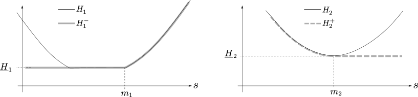
Figure 1: Typical situation.

Proof.

We provide the proof for $H_{1}$ only, since it is the same for $H_{2}$. Notice first that obviously, by definition $H_{1}=\max(H_{1}^{-};H_{1}^{+})$.

Next, the minimum of the convex, coercive function $s\mapsto H_{1}(x,p^{\prime}+se_{N})$ is achieved at some $\bar{s}\in\mathbb{R}$ and then standard results of convex analysis show that the maximum which defines $H_{1}(x,p^{\prime}+\bar{s}e_{N})$ is attained for a control $\alpha_{*}\in A_{1}$ such that $b_{1}(x,\alpha_{*})\cdot e_{N}=0$. Hence we can use this specific control in the supremum for $H_{1}^{-}(x,p)$ and we deduce that $H_{1}^{-}(x,p)\geq\underline{H}_{1}$. A small modification of this argument shows also that $H_{1}^{+}(x,p)\geq\underline{H}_{1}$ (we need to add a little bit of controlability here because the supremum for $H_{1}^{+}$ requires $b\cdot e_{N}>0$, not $b\cdot e_{N}=0$).

Then, we have $H_{1}^{-}(x,p)\leq\underline{H}_{1}$ if $p_{N}\leq m_{1}$ since $s\mapsto H^{-}_{1}(x,p^{\prime}+se_{N})$ is increasing, and a similar argument shows that for $p_{N}\geq m_{1}$, $H^{+}_{1}(x,p)\leq\underline{H}_{1}$. Hence we deduce that

$$H_{1}(x,p)=\begin{cases}H_{1}^{+}(x,p)&\text{if }p_{N}\leq m_{1}\,,\\ H_{1}^{-}(x,p)&\text{if }p_{N}>m_{1}\,.\end{cases}$$

For $p_{N}>m_{1}$, the convex function $p_{N}\mapsto H_{1}(x,p^{\prime}+p_{N}e_{N})$ cannot have $0$ in its subdifferential (otherwise at such a point we would have a minimum point, which would contradict the definition of $m_{1}$) and therefore by the classical Mean Value Theorem for convex functions in $1-d$, this function is increasing for $p_{N}>m_{1}$. ∎

For any $x\in\mathbb{R}^{N}$, $p\in\mathbb{R}^{N}$ we define the Hamiltonians

$$\tilde{H}(x,p):=\max(H_{1}(x,p),H_{2}(x,p))$$ (A.1)

$$\tilde{H}^{\rm reg}(x,p):=\max(H_{1}^{-}(x,p),H_{2}^{+}(x,p))\;.$$ (A.2)

Remark A.2.

We notice that the Hamiltonian $\tilde{H}$ is convex and coercive in the $p$-variable (since it is the maximum of two convex and coercive Hamiltonians). Moreover the same properties hold for $\tilde{H}^{\rm reg}$ thanks to the structure of $H_{1}^{-}$ and $H_{2}^{+}$ proved in Lemma A.1.

We recall that the Hamiltonians $\tilde{H}$ and $\tilde{H}^{\rm reg}$ are convex and coercive in the $p$-variable (since we are taking the maximum of two convex Hamiltonians). Moreover, we have

$$H_{T}(x,p^{\prime})=\min_{s\in\mathbb{R}}\tilde{H}(x,p^{\prime}+se_{N})\,,$$ (A.3)

$${H}^{\rm reg}_{T}(x,p^{\prime})=\min_{s\in\mathbb{R}}\tilde{H}^{\rm reg}(x,p^{\prime}+se_{N})\,.$$ (A.4)

Indeed, equalities (A.3)-(A.4) follow from the definition of $H_{T}$ and ${H}^{\rm reg}_{T}$ (see Remark 3.2) and classical results in convex analysis. For a detailed similar argument see the proof of Theorem 3.3 case 1 in [2].

The next step consists in introducing the function

$$\phi(\lambda):=\tilde{H}^{\rm reg}(x,p^{\prime}+\lambda e_{N})\,.$$ (A.5)

We are going to describe the different types of situations for this function $\phi$ and the consequences for the values of $H_{T}(x,p^{\prime})$, ${H}^{\rm reg}_{T}(x,p^{\prime})$ and for the equations

$$H^{-}_{1}(x,p^{\prime}+\lambda_{1}e_{N})=A\quad\mbox{ and }\quad H^{+}_{2}(x,p^{\prime}+\lambda_{2}e_{N})=A,$$ (A.6)

which appear in the proof of Theorem 2.5. To do so, we introduce the functions $f_{1}(s):=H_{1}^{-}(x,p^{\prime}+se_{N})$ and $f_{2}(s):=H_{2}^{+}(x,p^{\prime}+se_{N})$. Since $f_{1}(s)\to+\infty$ as $s\to+\infty$ and remains bounded as $s\to-\infty$, while $f_{2}(s)\to+\infty$ as $s\to-\infty$ and remains bounded as $s\to+\infty$ (see Figure 1), there exists at least a solution of the equation $f_{1}(s)=f_{2}(s)$ and we denote by $s_{*}$ the minimal solution. By the monotonicity properties of $f_{1}$ and $f_{2}$, it follows that $f_{2}>f_{1}$ for $s<s^{*}$ while $f_{2}\leq f_{1}$ for $s\geq s^{*}$. Taking into account the flat portions of $H_{1}^{-}$ and $H_{2}^{+}$ where they reach their respective minimum, we arrive at the following complete description.

Lemma A.3.

$(i)$ There are three possible configurations.

• Case 1 : $s_{*}\leq m_{1}$ and $s_{*}\leq m_{2}$ where (see Fig. 2)

  $$\phi(\lambda)=\begin{cases}H_{2}^{+}(x,p^{\prime}+\lambda e_{N})&\text{if }\lambda<s_{*}\,,\\ \underline{H}_{1}(x,p^{\prime})&\text{if }\lambda\in[s_{*},m_{1}]\,,\\ H_{1}^{-}(x,p^{\prime}+\lambda e_{N})&\text{if }\lambda>m_{1}\,.\\ \end{cases}$$ (A.7)

• Case 2 : $s_{*}>m_{1}$ and $s_{*}\geq m_{2}$ where

  $$\phi(\lambda)=\begin{cases}H_{2}^{+}(x,p^{\prime}+\lambda e_{N})&\text{if }\lambda\leq m_{2}\,,\\ \underline{H}_{2}(x,p^{\prime})&\text{if }\lambda\in[m_{2},s_{*}]\,,\\ H_{1}^{-}(x,p^{\prime}+\lambda e_{N})&\text{if }\lambda\geq s_{*}\,.\\ \end{cases}$$ (A.8)

• Case 3 : $s_{*}>m_{1}$ and $s_{*}\leq m_{2}$ where (see Fig. 3)

  $$\phi(\lambda)=\begin{cases}H_{2}^{+}(x,p^{\prime}+\lambda e_{N})&\text{if }\lambda<s_{*}\,,\\ H_{1}^{-}(x,p^{\prime}+\lambda e_{N})&\text{if }\lambda>s_{*}\,.\\ \end{cases}$$ (A.9)

$(ii)$ In Cases 1 & 2, we have

$${H}^{\rm reg}_{T}(x,p^{\prime})=\max(\underline{H}_{1}(x,p^{\prime}),\underline{H}_{2}(x,p^{\prime}))\;,$$

while, in Case 3, ${H}^{\rm reg}_{T}(x,p^{\prime})=H_{T}(x,p^{\prime})$.

$(iii)$ Finally, for any $A>\max(\underline{H}_{1}(x,p^{\prime}),\underline{H}_{2}(x,p^{\prime}))$ there exist a unique pair $\lambda_{2}<\lambda_{1}$ such that

$$H^{-}_{1}(x,p^{\prime}+\lambda_{1}e_{N})=A\quad\mbox{ and }\quad H^{+}_{2}(x,p^{\prime}+\lambda_{2}e_{N})=A$$

and the same equations hold with $H_{1}$ and $H_{2}$ instead of $H^{-}_{1}$ and $H_{2}^{+}$.

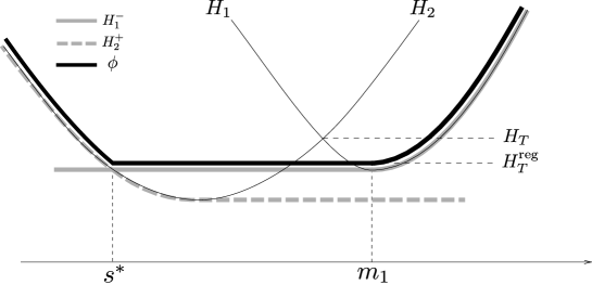
Figure 2: $H_{T}(x,p^{\prime})>{H}^{\rm reg}_{T}(x,p^{\prime})=\underline{H}_{2}(x,p^{\prime})$.

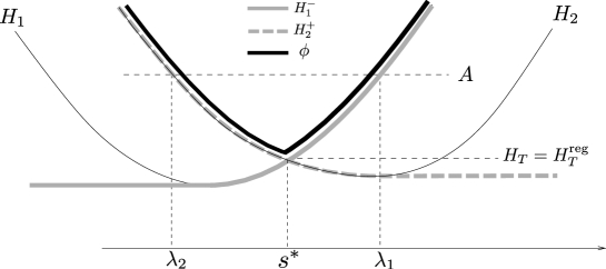
Figure 3: $H_{T}(x,p^{\prime})={H}^{\rm reg}_{T}(x,p^{\prime})$.

References

• [1] Yves Achdou, Fabio Camilli, Alessandra Cutrì, and Nicoletta Tchou. Hamilton-Jacobi equations constrained on networks. NoDEA Nonlinear Differential Equations Appl., 20(3):413–445, 2013.
• [2] G. Barles, A. Briani, and E. Chasseigne. A Bellman approach for two-domains optimal control problems in $\mathbb{R}^{N}$. ESAIM Control Optim. Calc. Var., 19(3):710–739, 2013.
• [3] G. Barles, A. Briani, and E. Chasseigne. A Bellman approach for regional optimal control problems in $\mathbb{R}^{N}$. SIAM J. Control Optim., 52(3):1712–1744, 2014.
• [4] Guy Barles. Solutions de viscosité des équations de Hamilton-Jacobi, volume 17 of Mathématiques & Applications (Berlin) [Mathematics & Applications]. Springer-Verlag, Paris, 1994.
• [5] Guy Barles and Emmanuel Chasseigne. (Almost) everything you always wanted to know about deterministic control problems in stratified domains. Netw. Heterog. Media, 10(4):809–836, 2015.
• [6] Alberto Bressan and Yunho Hong. Optimal control problems on stratified domains. Netw. Heterog. Media, 2(2):313–331 (electronic), 2007.
• [7] Cecilia De Zan and Pierpaolo Soravia. Cauchy problems for noncoercive Hamilton-Jacobi-Isaacs equations with discontinuous coefficients. Interfaces Free Bound., 12(3):347–368, 2010.
• [8] M. Garavello and P. Soravia. Representation formulas for solutions of the HJI equations with discontinuous coefficients and existence of value in differential games. J. Optim. Theory Appl., 130(2):209–229, 2006.
• [9] Mauro Garavello and Pierpaolo Soravia. Optimality principles and uniqueness for Bellman equations of unbounded control problems with discontinuous running cost. NoDEA Nonlinear Differential Equations Appl., 11(3):271–298, 2004.
• [10] Cyril Imbert and R Monneau. Quasi-convex Hamilton-Jacobi equations posed on junctions: the multi-dimensional case. $<$hal-01073954$>$ (second version), 2016.
• [11] Cyril Imbert and Régis Monneau. Flux-limited solutions for quasi-convex Hamilton-Jacobi equations on networks. 2016. $<$hal-00832545$>$ (fifth version), 2016.
• [12] Cyril Imbert, Régis Monneau, and Hasnaa Zidani. A Hamilton-Jacobi approach to junction problems and application to traffic flows. ESAIM Control Optim. Calc. Var., 19(1):129–166, 2013.
• [13] Cyril Imbert and Vinh Duc Nguyen. Generalized junction conditions for degenerate parabolic equations. 2016. $<$hal-01252891$>$ (first version), 2016.
• [14] Pierre-Louis Lions and Panagiotis Souganidis. Viscosity solutions for junctions: well posedness and stability. Rendiconti Lincei - matematica e applicazioni, 27(4):535–545, 2016.
• [15] Dirk Schieborn and Fabio Camilli. Viscosity solutions of Eikonal equations on topological networks. Calc. Var. Partial Differential Equations, 46(3-4):671–686, 2013.
• [16] Pierpaolo Soravia. Degenerate eikonal equations with discontinuous refraction index. ESAIM Control Optim. Calc. Var., 12(2):216–230 (electronic), 2006.