Localization-Delocalization Transitions in Bosonic Random Matrix Ensembles

Abstract

Localization to delocalization transitions in eigenfunctions are studied for finite interacting boson systems by employing one- plus two-body embedded Gaussian orthogonal ensemble of random matrices [EGOE(1+2)]. In the first analysis, considered are bosonic EGOE(1+2) for two-species boson systems with a fictitious ($F$) spin degree of freedom [called BEGOE(1+2)-$F$]. Numerical calculations are carried out as a function of the two-body interaction strength ($\lambda$). It is shown that, in the region (defined by $\lambda>\lambda_{c}$) after the onset of Poisson to GOE transition in energy levels, the strength functions exhibit Breit-Wigner to Gaussian transition for $\lambda>\lambda_{F_{k}}>\lambda_{c}$. Further, analyzing information entropy and participation ratio, it is established that there is a region defined by $\lambda\sim\lambda_{t}$ where the system exhibits thermalization. The $F$-spin dependence of the transition markers $\lambda_{F_{k}}$ and $\lambda_{t}$ follow from the propagator for the spectral variances. These results, well tested near the center of the spectrum and extend to the region within $\pm 2\sigma$ to $\pm 3\sigma$ from the center ($\sigma^{2}$ is the spectral variance), establish universality of the transitions generated by embedded ensembles. In the second analysis, entanglement entropy is studied for spin-less BEGOE(1+2) ensemble and shown that the results generated are close to the recently reported results for a Bose-Hubbard model.

I Introduction:

Transition from localization to delocalization phases in many-body quantum systems, due to inter particle interaction, has received a great attention in recent years Znid08 ; Pal-10 ; Khatami2012 ; JHB2012 ; RNand2015 ; Huse2007 ; Altman2015 . Now, a connection between the physics of the localization-delocalization transition and the physics of thermalization is well established Sengupta ; Rigol16 ; BISZ2016 . This is possible mainly due to major developments in the experimental study of many-particle quantum systems such as ultra-cold gases trapped in optical lattices Kondov2015 ; Schreiber2015 ; Bordia2015 and ions Smith2015 . It has been established that many-body interacting systems in which localization occurs, a phenomenon termed many-body localization (MBL), avoid thermalization due to the emergence of extensively many local integrals of motion. On the other hand, non-integrable quantum systems thermalize and the eigenstate thermalization hypothesis (ETH) is considered to be the underlying mechanism for thermalization ETH ; Rigol2008 . ETH essentially means that the expectation values of typical observables in the eigenstates of a many-body interacting system follow ergodicity principle. Various aspects related to the role of localization and chaos, statistical relaxation, eigenstate thermalization and ergodicity principle have been studied by many groups using lattice models of interacting spins (fermionic as well as bosonic systems) BISZ2016 ; Lea-12 ; Kollath ; ETH-1 ; ETH-2 ; Iz-PRL ; Manan .

Embedded Gaussian Orthogonal Ensemble (EGOE) of random matrices (for time-reversal and rotationally invariant systems) with one plus two-body interactions for fermions [called EGOE(1+2)], introduced in the past  MF ; Brody ; FI1 ; FI2 ; vkb2001 , are paradigmatic models to study the dynamical transition from integrability to chaos in isolated finite interacting many-body quantum systems vkb2001 ; PW-07 ; Ko-14 ; BISZ2016 . It is important to note that EGOE are generic, though analytically difficult to deal with, compared to the lattice spin models as the latter are associated with spatial coordinates (nearest and next-nearest neighbor interactions) only. Moreover, it is seen that the universal properties derived using EGOE apply to systems represented by lattice spin models. EGOE(1+2), as a function of the two-body interaction strength $\lambda$ (measured in units of the average spacing between the one-body mean-field single particle levels), exhibits three transition or chaos markers $(\lambda_{c},\lambda_{F_{k}},\lambda_{t})$: (a) as the two-body interaction is turned on, level fluctuations exhibit a transition from Poisson to GOE at $\lambda=\lambda_{c}$; (b) with further increase in $\lambda$, the strength functions (also known as the local density of states) make a transition from Breit-Wigner (BW) form to Gaussian form at $\lambda=\lambda_{F_{k}}>\lambda_{c}$; and (c) beyond $\lambda=\lambda_{F_{k}}$, there is a region of thermalization around $\lambda=\lambda_{t}$ where basis dependent thermodynamic quantities like entropy behave alike. For further details of the three chaos markers for EGOE(1+2) for spin-less fermion systems, see Ko-14 ; KoReta . It was also established that interacting fermion systems with fermions carrying spin (${\bf s}=1/2$) degree of freedom giving EGOE(1+2)-${\bf s}$ also exhibit these three transition markers and their spin dependence was also deduced Ma-PRE ; the propagator of the spectral variances explains the spin dependence. It is important to add that the transitions mentioned above are inferred from large number of numerical calculations and they are well verified to be valid around the center of the spectrum and extend in to the region within $\pm 2\sigma$ to $\pm 3\sigma$ from the center ($\sigma$ is the spectral width), i.e. in the bulk part of the spectrum. Also, the chaos markers are in general energy dependent; see Section III for an example. One observes deviations in the spectrum ends and this may be due to the the fact that the eigenvalue density generated by EGOE(1+2) is only asymptotically a Gaussian MF ; Ko-14 .

For bosonic systems, embedded Gaussian orthogonal ensembles of one- plus two-body interactions [denoted by BEGOE(1+2)] for finite isolated interacting spin-less many-boson systems have been analyzed in detail Pa-00 ; Ag-01 ; Ag-02 ; Ch-0304 ; Ch-PLA , as they are generic models for finite isolated interacting many-boson systems. For $m$ bosons in $N$ single particle (sp) states, in addition to the dilute limit (defined by $m\rightarrow\infty$, $N\rightarrow\infty$, $m/N\rightarrow 0$), another limiting situation, namely the dense limit (defined by $m\rightarrow\infty$, $N\rightarrow\infty$, $m/N\rightarrow\infty$) is also possible. Such a limiting situation is absent for fermion systems. Hence the focus was on the dense limit in BEGOE investigations Pa-00 ; Ag-01 ; Ag-02 ; Ch-0304 ; Ch-PLA . In the strong interaction limit, two-body part of the interaction dominates over one-body part and therefore BEGOE(1+2) reduces to BEGOE(2). In the dense limit, the eigenvalue density takes Gaussian form irrespective of the strength ($\lambda$) of the two-body interaction for these ensembles Pa-00 ; Ag-02 ; KP-80 . Just as spin-less fermionic EGOE(1+2), the BEGOE(1+2) also exhibits, as $\lambda$ increases, three chaos markers $(\lambda_{c},\lambda_{F_{k}},\lambda_{t})$. See Ch-0304 ; Ch-PLA ; Ko-14 for further details.

Going beyond spin-less boson systems, very recently BEGOE for two species boson systems with a fictitious $F$ spin-1/2 degree of freedom [called BEGOE(1+2)-$F$] Ma-F and for a system of interacting bosons carrying spin-one degree of freedom [called BEGOE(1+2)-$S1$] Deota-S1 are introduced and their spectral properties are analyzed in detail. Here, it is important to note that the $F$-spin for bosons is similar to the $F$-spin in the proton-neutron interacting boson model (pnIBM) of atomic nuclei Ia-87 ; Ca-05 . Similarly, BEGOE(1+2)-$S1$ is an important extension to apply BEGOE to spinor BEC discussed in Pe-10 ; PRA . The purpose of the present paper is firstly to establish universality of the localization-delocalization transitions generated by embedded ensembles by showing that BEGOE(1+2)-$F$ generates $\lambda_{F_{k}}$ and $\lambda_{t}$ transition markers (in addition to the $\lambda_{c}$ marker studied in Ma-F ) just as in the fermionic ensembles, without and with spin, and bosonic ensembles without spin. Secondly, going beyond the previous analysis of embedded ensembles, here for the first time, the bipartite entanglement entropy is studied using embedded ensemble for spin-less boson systems and shown that the results are close to those obtained recently using Bose-Hubbard models.

The paper is organized as follows. In Section II, briefly introduced is the BEGOE(1+2)-$F$ model. Section III is on the $\lambda_{F_{k}}$ marker and gives the results for BW to Gaussian transition in strength functions. Results for the participation ratio (PR) and the information entropy ($S^{\mbox{info}}$) are described in Section IV. Section V deals with the thermalization $\lambda_{t}$ marker using information entropy. In Section VI, the bipartite entanglement entropy ($S^{EE}$) is studied and correlations of it with PR are presented. Finally, Section VII gives some concluding remarks. In Appendix A, for easy reference, collected are the definitions of strength functions, PR and $S^{\mbox{info}}$ and also some EGOE formulas that are used in the analysis presented in Sections III–V.

II Embedded bosonic ensembles with $F$-spin:

II.1 Definition and construction:

Consider a system with $m$ ($m>2$) bosons distributed in $\Omega$ number of sp orbitals each with spin ${\bf f}=\frac{1}{2}$. With $\Omega$ number of orbital degrees of freedom and two spin ($m_{\bf f}=\pm\frac{1}{2}$) degrees of freedom, the total number of sp states is $N=2\Omega$. The sp states for bosons are denoted by $\left.\left|i,m_{\bf f}=\pm\frac{1}{2}\right.\right\rangle_{s}$ with $i=1,2,\ldots,\Omega$ and the two particle symmetric states are denoted by $\left.\left|(ij)f,m_{f}\right.\right\rangle$ with the two particle spin $f=0$ or $1$. For one plus two-body Hamiltonians preserving $m$ particle spin $F$, the one-body Hamiltonian is $h(1)=\sum_{i}\epsilon_{i}\;n_{i}$, where the orbits $i$ are doubly degenerate, $n_{i}$ are number operators and $\epsilon_{i}$ are sp energies. Similarly the two-body Hamiltonian $V(2)$ is defined by the two-body matrix elements $V^{f}_{ijkl}={{}_{s}}\left\langle(kl)f,m_{f}\mid V(2)\mid(ij)f,m_{f}\right\rangle_{s}$ and they are independent of the $m_{f}$ quantum number. Thus, $V(2)=V^{f=0}(2)+V^{f=1}(2)$; the sum here is a direct sum with dimensions $\Omega(\Omega-1)/2$ and $\Omega(\Omega+1)/2$ respectively. Then BEGOE(1+2)-$F$ is defined by the Hamiltonian $H$ that preserves total $m$ particle spin $F$,

$$H=h(1)+\lambda V(2)\;.$$ (1)

Here, $\lambda$ is the strength of the two-body interaction $V(2)$. In principle, it is possible to use a more general $H$ with the strengths of the $V^{f=0}(2)$ and $V^{f=1}(2)$ to be different but this is not considered in this paper. It is important to note that the $m$ particle states can be classified according to the algebra $U(N)\supset U(\Omega)\otimes SU(2)$ with $SU(2)$ generating spin $F$. As $H$ preserves $F$, it is a scalar in spin $SU(2)$ space. This recognition allows one to derive formulas for the spectral variances discussed in Sec. II.2.

BEGOE(1+2)-$F$ is generated by the action of $H$ on many-particle basis states with $V^{f=0}(2)$ and $V^{f=1}(2)$ being independent GOEs in two-particle spaces; variances of the matrix elements in both GOEs are taken to be unity. Given the sp energies and the two-body matrix elements, the many-particle Hamiltonian $H$ is first constructed in the $M_{F}=M_{F}^{min}$ [$M_{F}^{min}=0(\frac{1}{2})$ for $m$ even(odd)] representation using the spin-less BEGOE formalism and then states with a given $F$ are projected using the spin projection operator $F^{2}$; see Ma-PRE ; Ma-F for details. Thus, the many-particle Hamiltonian $H$ will be a block diagonal matrix with each diagonal block corresponding to a given spin $F$ Ma-F .

Earlier, by studying the distribution $P(r)$ of the ratio of consecutive level spacings, that do not require spectral unfolding and introduced by Oganesyan and Huse Huse2007 , to investigate many-body localization Huse2007 ; OPH2009 , it was demonstrated that the embedded ensembles including BEGOE(1+2)-$F$ exhibit GOE level fluctuations for sufficiently strong interaction strength $\lambda$ CK2013 ; CHK2014 . Note that Atas et al. ABGR-2013 derived expressions for the $P(r)$ distribution for the classical GOE, GUE and GSE ensembles of random matrices. In addition, using the nearest neighbor spacing distribution (NNSD), it was shown that BEGOE(1+2)-$F$ exhibits Poisson to GOE transition as the interaction strength $\lambda$ is increased and the transition marker $\lambda_{c}$ is found to decrease with increasing $F$-spin. Moreover, the ensemble-averaged spectral variance explains the decrease in $\lambda_{c}$ with increasing $F$ Ma-F . With $\Omega=4$, $m=10$, the $\lambda_{c}$ values for these ensembles are found to be $0.039$, $0.0315$ and $0.0275$ for $F=0$, $2$ and $5$ respectively. Going beyond these investigations where only eigenvalues were analyzed, in the present study, our focus is on eigenfunctions. Numerical calculations are carried out using fixed set of sp energies $\epsilon_{i}=i+1/i$ as in our previous studies Ma-PRE ; Ma-F and generated 100 member BEGOE(1+2)-$F$ ensembles with $\Omega=4$ and $m=10$. The $H$ matrix dimensions for various $F$ values are $d(m,\Omega,F)=196,540,750,770,594$ and $286$ for $F=0-5$; $\sum_{F=F_{min}}^{F_{max}}(2F+1)\;d(m,\Omega,F)={{2\Omega+m-1}\choose{m}}$.

II.2 BEGOE(1+2)-$F$ spectral variances and their spin dependence:

Here, we will briefly discuss the structure of the ensemble averaged spectral variance for BEGOE(1+2)-$F$ as they will provide an analytical understanding of the spin dependence of the chaos markers. With fixed $h(1)$, the ensemble averaged spectral variance $\overline{\sigma^{2}_{H}(m,F)}$ follows simply from Eq. (1),

$$\overline{\sigma^{2}_{H}(m,F)}=\sigma^{2}_{h(1)}(m,F)+\lambda^{2}\;\overline{\sigma^{2}_{V(2)}(m,F)}\;\;.$$ (2)

Note that ‘overline’ denotes ensemble average. The $\sigma^{2}_{h(1)}(m,F)$ and $\sigma^{2}_{V(2)}(m,S)$ are the variances generated by the $h(1)$ part and the perturbation $V(2)$ respectively. Now, for a uniform sp spectrum having unit average level spacing, the $\sigma^{2}_{h(1)}(m,F)$ is given as Ma-F ,

$$\sigma^{2}_{h(1)}(m,F)=\frac{1}{12}\Big{[}m(\Omega-2)(\Omega+m/2)+2\Omega F(F+1)\Big{]}\;.$$ (3)

Similarly, the ensemble averaged variance generated by the two-body interaction $V(2)$ is given as $\overline{\sigma^{2}_{V(2)}(m,F)}=Q(\Omega,m,F)$. Explicit formula, derived using trace propagation methods, for the variance propagator $Q(\Omega,m,F)$ is given in Appendix-A and it is taken from Ma-F ; Ko-14 . The propagator $Q(\Omega,m,F)$ (see Fig. 6 in Ma-F ), for bosonic systems, increases with increasing spin $F$. This trend is opposite for fermionic systems Ma-PRE .

III Transition in strength functions: $\lambda_{F_{k}}$ marker

The effects of localization-delocalization transition in the eigenfunctions reflect in the degree of mixing of the eigenfunctions of the system. Eigenfunction structure is understood usually in terms of the shape of the strength functions or local density of states $F_{k}(E)$ where $k$ is an initial basis state in which the system is prepared. Note that (see Appendix-A for details) $F_{k}(E)$ gives spreading of the $k$ states over the eigenstates, i.e. distribution of the square of the expansion coefficients $C_{k}^{E}$ in $\left.|k\right\rangle=\sum_{E}C_{k}^{E}\left.|E\right\rangle$. In the BEGOE(1+2)-$F$ study, we take the $k$ states to be the eigenstates of both $h(1)$ and $F^{2}$ operators; see KCS2006 ; Tureci2006 ; kaplan2000 ; Jacquod2001 ; papenbrock2002 . Our interest is to obtain the ensemble averaged form of the strength functions. Towards this end, eigenvalues $E$ and the $k$-energies $\xi_{k}$ ,for each member, are made zero centered and scaled to the width [$\sigma_{H}(m,F)$] of the eigenvalue spectrum. The new energies are called $\hat{E}$ and $\hat{\xi_{k}}$, respectively. Now, for each member, all ${|C_{k}^{E}|}^{2}$ are summed over the basis states $k$ with energy $\hat{\xi_{k}}$ in the energy window $\hat{\xi^{c}_{k}}\pm\Delta_{k}$. Then, the ensemble averaged $F_{k}(\hat{E})$ vs $\hat{E}$ are constructed as histograms by applying the normalization condition $\int F_{k}(\hat{E})d\hat{E}=1$. We have chosen $\Delta_{k}=0.025$ for $\lambda<0.06$ and beyond this $\Delta_{k}=0.1$. Figure 1 shows ensemble averaged strength functions $F_{k}(E)$ for the $k$ states averaged over $\hat{\xi^{c}_{k}}-\Delta_{k}\leq\hat{\xi_{k}}\leq\hat{\xi^{c}_{k}}+\Delta_{k}$ with $\hat{\xi^{c}_{k}}=0$. Results are shown for various values of $\lambda$ for the system with $m=10$ bosons in $\Omega=4$ sp orbitals and spin $F=0$, 3 and 5. Similarly, Figure 2 shows ensemble averaged strength function for $\hat{\xi^{c}_{k}}=-1,-1.5$ and $-2$ with three different values of $\lambda$ and for spins $F=3$ and $F=5$. The results clearly display transition from BW form to the Gaussian form, as the strength of the two-body interaction $\lambda$ increases beyond $\lambda_{c}(F)$. With $h(1)$ alone, that is for $\lambda=0$, the basis states become the eigenstates and therefore the strength functions are $\delta$-functions. With increase in $\lambda$, the states begin to spread and configurations begin to mix due to the two-body interaction, and the strength functions acquire BW form (see Eq. A-3). With further increase in $\lambda$, the strength functions start becoming Gaussian in nature (see Eq. (A-4). Note that the BW form implies weak de-localization and Gaussian form implies full delocalization. For BEGOE (or EGOE), full delocalization (or fully chaotic) is in a energy shell but not in the whole unperturbed basis and this aspect will be elaborated at the end of the next Section.

In order to quantify the BW to Gaussian transition, used is the BW to Gaussian interpolating student-$t$ distribution with a shape parameter $\alpha$; see Eq. (A-5) and Refs. Angom2004 ; Ma-PRE for more details regarding the $t$-distribution. The continuous red curves in Fig. 1 are obtained by fitting the strength function histograms with Eq. (A-5) and the values of the shape parameter $\alpha$ are given in the figure. Note that the results in Fig. 1 are for $\hat{\xi^{c}_{k}}=0$. As seen from the results, the fits are excellent over a wide range of $\lambda$ values. The criterion $\alpha\sim 4$ defines the transition point $\lambda_{F_{k}}$ Angom2004 . Value of the parameter $\alpha$ increases slowly up to $\lambda_{F_{k}}$, then it increases sharply. For $\alpha>16$, the curves are indistinguishable from Gaussian. From the results in Fig. 1, it is seen that the transition point $\lambda_{F_{k}}$ is close to 0.06, 0.05 and 0.04 for $F$=0, 3 and 5 respectively. For a qualitative understanding of the variation of $\lambda_{F_{k}}$ with $F$ spin, we use the procedure adopted in the study of EGOE(1+2)-${\bf s}$ Ma-PRE , where the spreading width of the strength functions and the participation ratio (PR) are used to obtained the chaos marker in terms of the variance propagator Ma-PRE . For BEGOE(1+2)-$F$ we have,

$$\lambda_{F_{k}}(F)\propto\displaystyle\sqrt{\displaystyle\frac{m\Omega^{2}}{Q(\Omega,m,F)}}\;\;.$$ (4)

Thus, the marker $\lambda_{F_{k}}$ is essentially determined by the variance propagator $Q(\Omega,m,F)$. From the results in Fig. 6 in Ma-F , it is clear that $\lambda_{F_{k}}$ should decrease with $F$. This prediction is in agreement with the results shown in Fig. 1. Therefore, Eq. (4) gives a good qualitative understanding of $\lambda_{F_{k}}(F)$ variation with $F$ just as for $\lambda_{c}(F)$ shown in Ma-F . Turning to Figure 2, it can be argued that,, for the BEGOE system considered, the BW to Gaussian transition extends upto $\hat{\xi^{c}_{k}}=\pm 2$. From $-2$ and below the transition is slower and strength function is not symmetric. Due to the finiteness of the system, number of states below $\hat{\xi^{c}_{k}}=-2$ will be much smaller than those above $-2$. Also, as seen from Fig. 2, $\lambda_{F_{k}}(F)$ depends on $\hat{\xi^{c}_{k}}$ and its value increases as we go away from the center.

In order to understand further the structures due to delocalization of the eigenfunctions, we will consider the two standard measures, the participation ratio and information entropy in the next section; these are defined in Appendix-A.

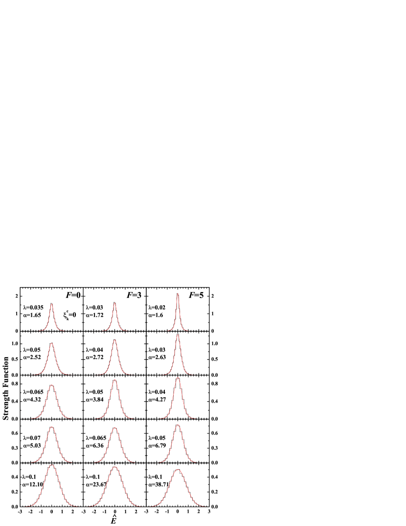
Figure 1: Strength functions for $k$ states averaged over $\hat{\xi^{c}_{k}}-\Delta_{k}\leq\hat{\xi_{k}}\leq\hat{\xi^{c}_{k}}+\Delta_{k}$ with $\hat{\xi^{c}_{k}}=0$. Strength functions are shown for five different values of $\lambda$ and they are for a 100 member BEGOE(1+2)-$F$ ensemble. Calculations are for $\Omega=4$, $m=10$ system with spins $F=0,3$ and $5$. Note that the width $\sigma_{F_{k}(m,F)}$ of the strength functions is different from the spectral width $\sigma_{H}(m,F)$. Continuous curves in the figures correspond to the $t$-distribution given by Eq. (A-5). See text for further details.

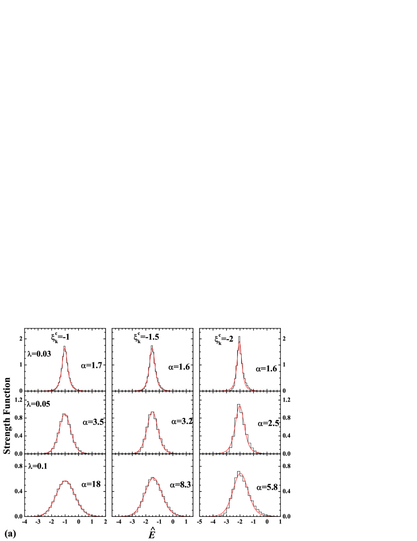
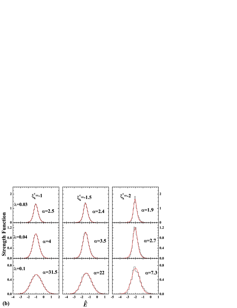
Figure 2: Histograms represent strength functions vs. normalized energy, for three different values of $\lambda$ using a 100 member BEGOE(1+2)-$F$ ensemble with $\Omega=4$, $m=10$ system. Strength function plots are obtained for $\hat{\xi^{c}_{k}}=-1,-1.5$ and $-2$ and results are shown for spins (a) $F=3$ and (b) $F=5$. Continuous curves in the figures correspond to the $t$-distribution given by Eq. (A-5). See text for further details. Results for $\hat{\xi^{c}_{k}}=1,1.5$ and $2$ are not shown in the figure as they are similar to those for $\hat{\xi^{c}_{k}}=-1,-1.5$ and $-2$ respectively.

IV Participation ratio and Information entropy

Participation ratio (PR) or number of principal components is a useful quantity to measure the degree of delocalization of a given eigenstate. The $\mbox{PR}(E)$ defined by Eq. (A-6) gives essentially the number of basis states $k$ that make up the eigenstate with energy $E$. Fig. 3 shows the variation of PR for the same 10 boson system used in generating Figs. 1 and 2 and for spins $F=0$ and 5. In the figures, continuous curves correspond to the BEGOE(1+2) formula given by Eq. (A-7) and the numerical ensemble averaged PR values are shown as red filled circles. One can see that for small values of $\lambda$, where the one-body part of the interaction is dominating with the spacing distribution is close to Poisson in character, the theoretical curve is, as expected, far away from the numerical results. With $\lambda=\lambda_{c}$ also, corresponding to the transition from Poisson to Wigner distribution for NNSD, the theoretical estimate for PR is above the ensemble averaged values. However, the ensemble averaged results are close to those given by Eq. (A-7) for $\lambda$ near or above $\lambda_{F_{k}}$. Thus Eq. (A-7) is good in the de-localized regime with $\lambda\mathrel{\mathchoice{\vbox{\offinterlineskip\halign{\hfil$\displaystyle#$\hfil\cr>\cr\sim\cr}}}{\vbox{\offinterlineskip\halign{\hfil$\textstyle#$\hfil\cr>\cr\sim\cr}}}{\vbox{\offinterlineskip\halign{ \hfil$\scriptstyle#$\hfil\cr>\cr\sim\cr}}}{\vbox{\offinterlineskip\halign{\hfil$\scriptscriptstyle# $\hfil\cr>\cr\sim\cr}}}}\lambda_{F_{k}}$.

Another statistical quantity closely related to PR is the information entropy $S^{\mbox{info}}(E)$ in the eigenfunctions; Eq. (A-9) gives the definition. Clearly, increase in information entropy implies more delocalization of the eigenstates. It is well demonstrated in casati98 ; horoi95 that the thermodynamics entropy defined by the state density, the information entropy in the eigenfunctions expanded in the mean-field basis and the single particle entropy defined by the mean occupation numbers of the sp states, all coincide for strong enough interaction but only in the presence of a mean field; i.e. in the chaotic domain ($\lambda>\lambda_{F_{k}}$) but with a mean field. In Fig. 3, numerical results for $S^{\mbox{info}}$ for the 10 boson system with $F=0$ and $5$ are compared with the results from the BEGOE(1+2) formula (see Eq. (A-10)) for the same values of $\lambda$ as used for PR. As seen from the figures, there is a good correlation between $S^{\mbox{info}}$ and PR results as expected Angom2004 ; Jacq-02 ; Varga . Also, for $\lambda\mathrel{\mathchoice{\vbox{\offinterlineskip\halign{\hfil$\displaystyle#$\hfil\cr>\cr\sim\cr}}}{\vbox{\offinterlineskip\halign{\hfil$\textstyle#$\hfil\cr>\cr\sim\cr}}}{\vbox{\offinterlineskip\halign{ \hfil$\scriptstyle#$\hfil\cr>\cr\sim\cr}}}{\vbox{\offinterlineskip\halign{\hfil$\scriptscriptstyle# $\hfil\cr>\cr\sim\cr}}}}\lambda_{F_{k}}$, theoretical results given by Eq. (A-10) are close to the ensemble averaged numerical results for different $F$ values. This again confirms that as $\lambda$ increases beyond $\lambda_{F_{k}}$ eigenstates start becoming fully delocalized (chaotic) and the meaning of full delocalization is discussed below. From the PR and $S^{\mbox{info}}$ results in Fig. 3, it is seen that the transition point $\lambda_{F_{k}}$ deduced in Section III corresponds to $\zeta\sim 0.75-0.8$.

Results in Fig. 3 show that even when $\lambda>>\lambda_{F_{k}}$, the eigenstates will not occupy the whole unperturbed basis and this is due to the fact that the interaction is two-body in nature (i.e. $2<<m$). In this situation, one can use the notion of delocalization in a ’enery shell’ whose width is defined by the interaction. Because of this, PR and information entropy in general will not reach the value given by full random matrices. This is confirmed by the results in Fig. 3 and also by Eqs. (A-7,A-10). It should noted that even for energies taken not close to the center, the eigenstates can be fully chaotic and delocalized in the energy shell, and not in the whole unperturbed basis. Quantitative results for the notion of energy shell and the width of the energy shell are obtained using banded random matrix ensembles by Casati et al. Cas-1 ; Cas-2 ; see also the discussion in BISZ2016 . For EGOE(1+2) or BEGOE(1+2), given a eigenstate with energy $E$, an estimate of the location and width of the energy shell follows from the results given in vkbrs01 . We will discuss this in the following section after examining the structure of the eigenstates with $\lambda$ increasing beyond $\lambda_{F_{k}}$.

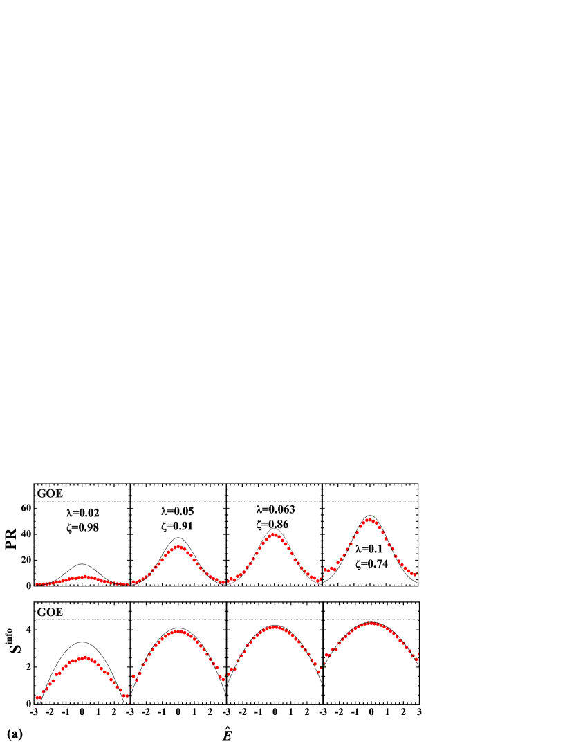
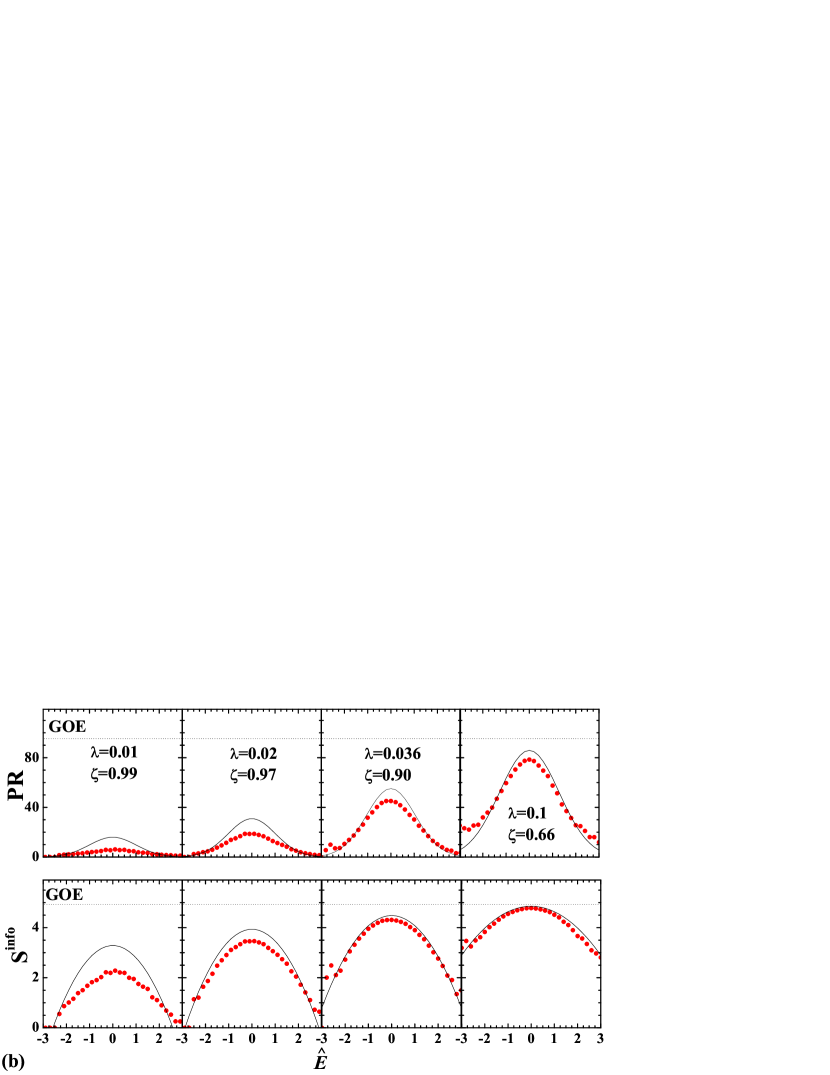
Figure 3: PR and $S^{\mbox{info}}$ vs. normalized energy $\hat{E}$ for a system of $m=10$ interacting bosons in $\Omega=4$ sp orbitals. Results are shown for (a) minimum spin $F=0$ and (b) maximum spin $F=5$. In each case 100 members are used. Ensemble averaged results are represented by red circles while continuous curves correspond to the theoretical estimates in the chaotic domain as given by Eqs. (A-7) and (A-10).

V Thermodynamic region: $\lambda_{t}$ marker

The thermodynamic region defined by $\lambda\sim\lambda_{t}$ is the region where any definition of the thermodynamic quantities such as entropy, temperature etc. gives the same result. Then, one can argue that in this region all wave functions look alike (similar to ETH). In fact, this is also the duality region for embedded ensembles Jacq-02 ; Angom2004 ; Ma-PRE . Just like for other embedded ensembles, for the BEGOE(1+2)-$F$ Hamiltonian, there are two choices of basis appear naturally. One is the mean-field basis defined by $h(1)$ and another is the infinite interaction strength basis defined by $V(2)$. To locate duality or equivalently for establishing the thermodynamic region, we compute information entropy $S^{\mbox{info}}(E)$ in these two basis. At $\lambda=\lambda_{t}$, the spreadings produced by $h(1)$ and $V(2)$ are equal giving the correlation coefficient $\zeta$ to be $\zeta^{2}(\lambda_{t})=1/2$ Angom2004 ; see Eq. (A-8) for the definition of $\zeta^{2}$ and Eqs. (A-7) and (A-10) for the role of $\zeta^{2}$ in PR and $S^{\mbox{info}}(E)$. Hence, putting $\zeta^{2}=1/2$ in Eq. (A-10) gives the basis independent expression $S_{\lambda_{t}}^{\mbox{info}}(E)=\ln(0.48d)+\ln\sqrt{1/2}+\frac{(1-E^{2})}{4}$. To identify $\lambda_{t}$, we use a $\chi^{2}$ measure giving sum of the squares of the deviations between numerically obtained $S^{\mbox{info}}(E)$ in $h(1)$ basis and $V(2)$ basis with the expression (see Eq. A-10)for $S_{\lambda_{t}}^{\mbox{info}}(E)$:

$$\chi^{2}=\displaystyle\int_{-\infty}^{\infty}\mathrm{d}E\;\left[{\{R_{\lambda_{t}}^{E}-R_{h(1)}^{E}\}^{2}+\{R_{\lambda_{t}}^{E}-R_{V(2)}^{E}\}^{2}}\right]\;.$$ (5)

Here $R_{\alpha}^{E}=\exp[S_{\alpha}^{\mbox{info}}(E)-S^{\mbox{info}}_{GOE}]$ with $\alpha$ representing $h(1)$ or $V(2)$. The minimum value of $\chi^{2}$ gives the $\lambda_{t}$. Figure 4 shows variation of $\chi^{2}$ (red stars) with the interaction strength $\lambda$ for a 100 member BEGOE(1+2)-$F$ ensemble. Used here is the ensemble for $\Omega=4$,$m=10$ and the results are shown for $F$ spin values 0, 3 and 5. It can be seen that for the present example, $\lambda_{t}\simeq 0.11$ for $F$=0, $\lambda_{t}\simeq 0.10$ for $F$=3 and $\lambda_{t}\simeq 0.086$ for $F$=5. The two vertical doted lines, in each plot, indicate the respective positions of $\lambda_{F_{k}}$ and $\lambda_{t}$. For $\lambda<\lambda_{t}$, the $S_{h(1)}^{\mbox{info}}$ values are higher and $S_{V(2)}^{\mbox{info}}$ values are smaller compared to $S_{\lambda_{t}}^{\mbox{info}}$ and for $\lambda>\lambda_{t}$, the situation is reversed giving $\chi^{2}>0$. The values of entropy, in the two basis coincide with $S_{\lambda_{t}}^{\mbox{info}}$ at $\lambda=\lambda_{t}$ giving $\chi^{2}\sim 0$. In Fig. 4, ensemble averaged values of $\zeta^{2}$ (blue circles) are also shown for each $F$ spin. It is clear from the figure that for smaller $\lambda$ ($\lambda\leq\lambda_{c}$), $\zeta^{2}$ is close to $1$ and as $\lambda$ increases, $\zeta^{2}$ goes on decreasing smoothly. It is seen from the figure that the condition $\zeta^{2}(\lambda_{t})=0.5$ gives the same values for the marker $\lambda_{t}$ as obtained using information entropy.

Qualitative understanding of the variation of $\lambda_{t}$ with $F$ is obtained using the fact that at $\lambda=\lambda_{t}$ we have $\zeta^{2}(\lambda_{t})=0.5$. This leads to the condition $\sigma^{2}_{h(1)}(m,F)=\lambda^{2}_{t}\;Q(\Omega,m,F)$. Then, for BEGOE(1+2)-$F$, using Eq. (3) for $\sigma^{2}_{h(1)}$ will give,

$$\lambda_{t}(F)\propto\displaystyle\sqrt{\displaystyle\frac{\sigma^{2}_{h(1)}(m,F)}{Q(\Omega,m,F)}}\;.$$ (6)

Eq. (6) gives a good qualitative understanding of $\lambda_{t}$ variation with $F$. Before going further, let’s add that even when $\lambda$ value is large, numerical results in Fig. 3 show that close to the bottom of the spectrum thermalization is absent and the corresponding eigenstates are not fully chaotic. For a more complete understanding of the structure of the ground state region generated by embedded ensembles, numerical results with much larger values of $(m,\Omega)$ are needed and this is future studies.

Returning to the energy shell mentioned at the end of Section IV, in the thermodynamic region, form of the strength functions will be Gaussian and the eigenstates are fully (chaotic) delocalized in the energy shell. Using Eq. (1) of vkbrs01 , we have the result that the distribution of $\left|C^{E}_{k}\right|^{2}$ vs $\xi_{k}$ for a fixed $E$ is a Gaussian, in the thermalization region, with center at $\zeta\hat{E}$ and width $\sqrt{1-\zeta^{2}}$. Note that $1-\zeta^{2}$ is the spectral variance generated by the two-body part of the Hamiltonian (measured in units of the total spectral variance). As $\zeta^{2}=1/2$ in the thermalization region, it can be argued that the width (energy span) of the energy shell is $\sim 2\sqrt{1-\zeta^{2}}\sigma_{H}=\sqrt{2}\sigma_{H}$. Moreover, for $\lambda\leq\lambda_{F_{k}}$ as discussed before $\zeta^{2}>>1/2$ and therefore the eigenstates are much less delocalized than in the thermodynamic region. For a better quantitative understanding of the energy shell in embedded ensembles calls for a more rigorous mathematical treatment of these ensembles and/or numerical investigations with much larger values for $(m,\Omega)$. Clearly, this needs to be investigated but it is outside the scope of the present paper.

In summary, the above results along with the previous studies, for EGOE(1+2), EGOE(1+2)-${\bf s}$ and BEGOE(1+2), establish universality of the BW–Gaussian transition in strength functions and the region of thermalization marked by $\lambda_{F_{k}}$ and $\lambda_{t}$ respectively, both for bosonic and fermionic systems (with and without good quantum numbers). Similar structures were obtained using spin models employed by Lea Santos and others Rigol16 ; BISZ2016 and thus it is plausible to conclude that embedded ensembles are generic models for isolated finite interacting many-particle quantum systems.

Going further, in the next section, we will study entanglement entropy within embedded ensembles for spin-less boson systems. The entanglement measures, introduced in the context of Quantum Information Science, are used to characterize complexity in quantum many-body systems. Entanglement and delocalization are found to be strongly correlated for disordered spin-1/2 lattice systems Br-08 ; Pi-08 .

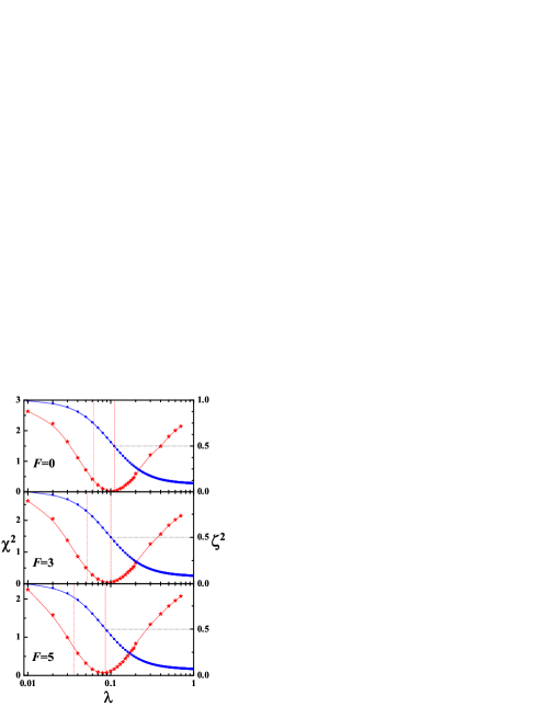
Figure 4: Variation of $\chi^{2}$ (red stars) and $\zeta^{2}$ (blue circles) as a function of the interaction strength $\lambda$, calculated for a 100 member BEGOE(1+2)-$F$ ensemble with $\Omega=4$,$m=10$ are shown for $F$ spin values 0, 3 and 5. The $\lambda_{t}$ marker for the thermodynamic region corresponds to $\chi^{2}=0$ and $\zeta^{2}=0.5$. The vertical red doted and dashed lines in each panel indicate the respective positions of $\lambda_{F_{k}}$ and $\lambda_{t}$.

VI Entanglement entropy in embedded ensembles

The bipartite entanglement entropy ($S^{EE}$) is a measure of the strength of quantum correlations between two parts of a many-body system. Consider an eigenstate with energy $E$, $|E\rangle$. Then, the full density matrix is given by $\rho(E)=|E\rangle\langle E|$. Let the system is divided into two parts $A$ and $B$ giving partition of its Hilbert space ${\mbox{\boldmath$H$}}={\mbox{\boldmath$H$}}_{A}\otimes{\mbox{\boldmath$H$}}_{B}$, where ${\mbox{\boldmath$H$}}_{A}$ and ${\mbox{\boldmath$H$}}_{B}$ are the Hilbert subspaces respectively. Now, an eigenstate is said to be separable if it can be written as $|E\rangle=|a_{E}\rangle\otimes|b_{E}\rangle$. Here, $|a_{E}\rangle$ and $|b_{E}\rangle$ are the basis states residing in the Hilbert subspaces ${\mbox{\boldmath$H$}}_{A}$ and ${\mbox{\boldmath$H$}}_{B}$ respectively. A state $|E\rangle$ is said to be entangled if it is not separable. The $S^{EE}$ between the partitions $A$ and $B$, in the eigenstate $|E\rangle$, is given by,

$$S^{EE}(E)=-Tr\rho_{A}(E)\log{\rho_{A}(E)}=-\sum_{\mu}\tau_{\mu}(E)\log{\tau_{\mu}(E)}.$$ (7)

Where $\rho_{A}(E)=Tr_{B}\rho(E)$ is the reduced density matrix of the $A$ part, obtained from the full density matrix $\rho(E)$ by tracing out $B$ degrees of freedom and $\tau_{\mu}(E)$ are the eigenvalues $\rho_{A}(E)$. For a separable state $S^{EE}=0$ while for a maximally entangled state $S^{EE}_{max}=\log d_{min}$, where $d_{min}=\min(d_{A},d_{B})$; $d_{A}$ and $d_{B}$ are the dimensionalities of the Hilbert subspaces ${\mbox{\boldmath$H$}}_{A}$ and ${\mbox{\boldmath$H$}}_{B}$ respectively. As in the definition of the $\rho(E)$, both self-correlations as well as cross-correlations between the coefficients $C^{E}_{k}$ are taken into account, unlike the PR and information entropy where the cross-correlations are neglected, the $S^{EE}$ is independent of the basis states. However, it does depend on the partition.

In Figure 5 shown are ensemble averaged results for $S^{EE}$ as a function of the normalized energies for various values of $\lambda$ in $H=h(1)+\lambda V(2)$. The systems considered are: (a) $m=10$ spin-less bosons in $N=4$ sp states; (b) $m=8$ spin-less bosons in $N=8$ sp states. See Ch-0304 for details of these BEGOE(1+2)ensembles. The last panel in both Fig. 5(a) and 5(b) are for BEGOE(2) only. In the present study, the $S^{EE}$ is obtained between two equal partitions of sp states. Then, $C^{E}_{k}$ changes to $C^{E}_{k_{A},k_{B}}$ and $\rho_{A}(E)$ is given by $\sum_{k_{B}}\,C^{E}_{k_{A},k_{B}}C^{E}_{k^{\prime}_{A}k_{B}}$. It can be clearly seen from Fig. 5 that for small $\lambda$, small $S^{EE}$ values are found in the tails of the spectrum while large as well as small $S^{EE}$ values are found in the middle part of the spectrum. As $\lambda$ increases, the $S^{EE}$ varies smoothly with energy. For sufficiently large $\lambda$, large $S^{EE}$’s in the middle part and small $S^{EE}$’s in the tails of the spectrum are found. This behavior can be understood as follows: For $\lambda=0$, with $h(1)$ part only, the basis states ($|k\rangle$) themselves are the eigenstates ($|E\rangle$) and hence the eigenstates are separable giving $S^{EE}=0$ for all the eigenstates. As soon as the interaction is switched on, the basis states begin to spread and the configurations start to mix due to the two-body interaction. At this point, the cross-correlations in the $\rho(E)$ start growing leading to mixing of the subspaces weakly and hence resulted into entangled eigenstates with non-zero but low $S^{EE}$ values. As in this region, the structure of eigenstates is not chaotic enough, leading to strong variation in $C^{E}_{k}$ and thus in the $\rho(E)$ leading to stronger variation in $S^{EE}$ values over the ensemble and particularly in the middle part of the spectrum. Then, one may argue that the eigenstates near the tails show area-law behavior, while those in the middle part show both area-law and volume-law behavior; for area and volume-laws for $S^{EE}$ see ee-area . With further increase in $\lambda$, more and more basis states contribute to the eigenstates leading to increase in $S^{EE}$ values. Here, reduction in the fluctuations leads to smooth variation of $S^{EE}$ with energies. For sufficiently stronger $\lambda$, the eigenstates, in the middle of the spectrum, become fully chaotic and the cross-correlations in the $\rho(E)$ are stronger enough to mix the subspaces completely giving maximum $S^{EE}$ value. As chaos sets in fast in the eigenstates in the middle part of the spectrum compared to the region near the ground state, larger values of $S^{EE}$ are generated in the middle part of the spectrum and small $S^{EE}$ values in the tail region of the spectrum. This suggests that the eigenstates have area-law like character near the spectral tails while volume-law like character in the middle part. The results here are in good agreement with those obtained in alba09 ; wouter2015 .

Following wouter2015 , we are further motivated to compare PR and $S^{EE}$. In Fig. 6, the scatter plots of $S^{EE}$ vs. PR for all the eigenstates are shown for one typical member of each of the two ensembles considered in Fig. 5. Note that $\mbox{PR}(E)=\{d\sum_{k}|C^{E}_{k}|^{4}\}^{-1}$ where $d$ is the dimension of the $H$ matrix. For ($m=4,N=10$), $d=286$ while for ($m=8,N=8$), $d=6435$. The PR values are plotted on a logarithmic scale. In the plots, the middle 80% eigenstates of the spectrum are shown using blue dots while remaining 10% of eigenstates from both ends of the spectrum are shown using red dots. The difference between the nature of middle part and the tails of the spectrum is clearly visible. For weak interaction strength $\lambda$, both PR and $S^{EE}$ values are much smaller than the random-state predictions for all the eigenstates. With increase in $\lambda$, PR and $S^{EE}$ values drift towards the random-state expectation values for more and more eigenstates from the middle part of the spectrum. With further increase in $\lambda$, the eigenstates in the middle part become fully chaotic leading to clustering of both PR and $S^{EE}$ near the random-state expectation values. The eigenstates near both the tails of the spectrum have much smaller values for these quantities. The straight lines in each of the the Fig. 6 are obtained by Orthogonal Distance Regression (ODR) to the full data sets wouter2015 . The BEGOE(1+2) results obtained in Figs. 5(b) and 6(b) show strikingly similar structure as obtained using Bose-Hubbard model in wouter2015 . This further confirms that BEGOE generates generic results for localization-delocalization transitions in finite interacting quantum systems.

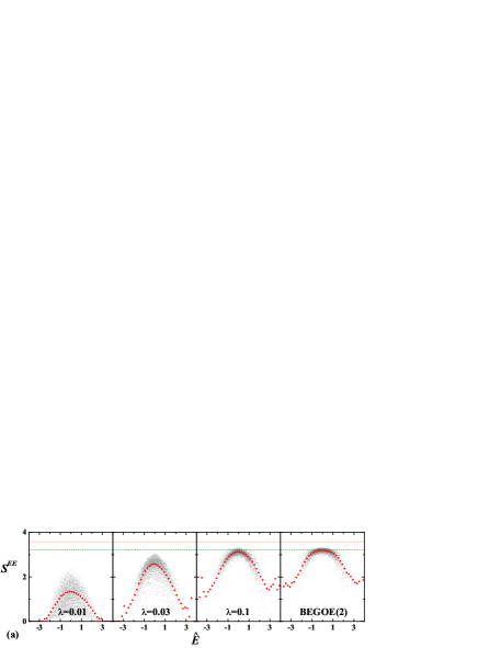
Figure 5: Ensemble averaged entanglement entropy ($S^{EE})$ vs. normalized energy $\hat{E}$ for various values of $\lambda$ are shown by red circles; (a) with $m=10$ spin-less bosons in $N=4$ sp states and (b) with $m=8$ spin-less bosons in $N=8$ sp states. In (a) each case 100 members are used and in (b) each case 5 members are used. The ensemble average is carried out by making the spectra of each member of the ensemble zero centered and scaled to unit width. Data points of a few members are also shown (small dots). The entanglement partition is between two equal halves of the sp states. The red dashed and red doted lines indicate the $S^{EE}_{GOE}$ and maximal $S^{EE}$, $S^{EE}_{max}$ respectively. For ($m=10,N=4$) example, $S^{EE}_{GOE}=3.23$ and $S^{EE}_{max}=\log{36}$, while for ($m=8,N=8$) example, $S^{EE}_{GOE}=4.38$ and $S^{EE}_{max}=\log{105}$. The last plots in both (a) and (b) are for BEGOE(2) only.

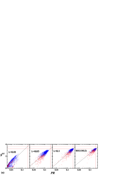
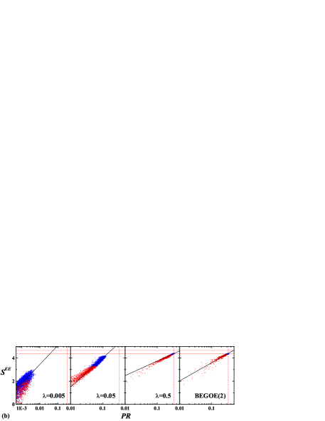
Figure 6: Scatter plots of entanglement entropy $S^{EE}$ vs. participation ratio (PR) for (a) with $m=10$ spin-less bosons in $N=4$ sp states and (b) with $m=8$ spin-less bosons in $N=8$ sp states. Data points for a single member of the ensembles are shown. The blue points indicate middle 80% eigenstates of the spectrum while the red dots represent 10% eigenstates from either side of the tails of the spectrum. The vertical and horizontal red dashed lines indicate $\mbox{PR}_{GOE}$ and $S^{EE}_{GOE}$ respectively while the horizontal red doted lines indicate $S^{EE}_{max}$. The black straight lines are due to ODR fits to the full data sets.

VII Conclusions:

In the present paper, we have studied localization to delocalization transitions using various traditional measures, based on the structure of eigenfunctions, such as the shape of strength functions, participation ratio and information entropy, as a function of the two-body interaction strength ($\lambda$) in BEGOE(1+2)-$F$ Hamiltonian. It is demonstrated that BEGOE(1+2)-$F$ ensembles, in addition to Poisson to GOE transition in level fluctuations at $\lambda_{c}$ Ma-F , generate two more transition (chaos) markers namely, $\lambda_{F_{k}}$ ($>\lambda_{c}$) and $\lambda_{t}$ ($>\lambda_{F_{k}}>\lambda_{c}$) for BW to Gaussian transition in strength functions and the duality or thermodynamic region respectively. Also, the variance propagator $Q(\Omega,m,F)$ [given by Eqs. (A-11) and (A-12)] gives a good qualitative explanation for the $F$-spin dependence of these chaos markers. As $Q$ increases with $F$, and using this in Eqs. (4) and (6), establishes that $\lambda_{F_{k}}$ and $\lambda_{t}$ values will increase with $F$ just as $\lambda_{c}$ ($F=m/2$ corresponds to spin-less bosons). Hence, these results establish that the introduction of the spin quantum number preserves the general structures, generated by spin-less EGOE(1+2) (bosonic and fermionic) ensembles and EGOE(1+2)-${\bf s}$ ensemble for fermions with spin, as established previously Ma-PRE ; Ko-14 , although the actual values of the markers vary with the $m$-particle spin. In the literature, most of the results for localization to delocalization transitions were obtained using spin models (with fermions and hardcore bosons) and Bose-Hubbard model Rigol16 ; BISZ2016 . Now, we have demonstrated that embedded ensembles give similar results and they do form a good model to study localization to delocalization transitions.

In addition to the traditional measures, we have analyzed entanglement entropy for spin-less BEGOE(1+2) ensembles using all the eigenstates and presented the first results. For weak interaction strength $\lambda$, the states with low-entanglement and low-PR appear in whole part of the spectrum. While for sufficiently large interaction strength $\lambda$, larger values in the middle part of the spectrum and smaller near the tails of the spectrum for both PR and $S^{EE}$ are found. Also correlations between PR and $S^{EE}$ are analyzed qualitatively. All these results are consistent with those obtained in wouter2015 where Bose-Hubbard model has been employed. These show that generic features can be well described by two-body ensembles (embedded ensembles) as emphasized in Br-08 . One can also study ETH and many aspects of thermalization using embedded ensembles. Recently, some of these are numerically investigated using embedded ensembles in KoReta ; Haldar2016 . In addition, using the simpler EGOE(1) generated by a random one-body Hamiltonian (with both diagonal and off-diagonal matrix elements) for fermions, ETH has been proved analytically by computing correlations and entanglement entropies Mag-16 . Hence, it is interesting and important to investigate these using two-body and one plus two-body embedded ensembles. This exercise will be carried out in future. It is also possible to consider Hamiltonians giving in some extreme limits regular features and intermediately chaotic behavior by adding some other regular Hamiltonians to the EGOE Hamiltonian considered in this paper. This will be addressed in future.

APPENDIX A

Given a $m$-particle state $\left|k\right\rangle$ and its expansion in terms of the eigenstates $\left|E\right\rangle$ of the Hamiltonian $H$ with eigenvalues $E$,

$$\left|k\right\rangle=\displaystyle\sum_{E}C_{k}^{E}\left|E\right\rangle\;.$$ (A-1)

The strength function that corresponds to the state $\left|k\right\rangle$ is

$$F_{k}(E)=\sum_{E^{\prime}}{|C_{k}^{E^{\prime}}|}^{2}\;\delta(E-E^{\prime})=d\,\overline{|C_{k}^{E}|^{2}}\,\varrho(E)\;.$$ (A-2)

Here, $\overline{|C_{k}^{E}|^{2}}$ is the average of $|C_{k}^{E}|^{2}$ over the degenerate $E$ states, $d$ is the dimension of the $m$-particle space and $\varrho(E)$ is the normalized eigenvalue density. Energy $\xi_{k}$ of the states $\left|k\right\rangle$ are given by $\xi_{k}=\langle k|H|k\rangle$, the diagonal matrix element of $H$ in the $k$ basis. The BW form for the strength functions, with $\Gamma$ denoting the spreading width, is

$$F_{k}(E)=\displaystyle\frac{\Gamma}{2\pi}\,\displaystyle\frac{1}{(E-\xi_{k})^{2}+\displaystyle\frac{\Gamma^{2}}{4}}\;.$$ (A-3)

Similarly, with $\sigma^{2}$ giving the spectral variance, the Gaussian form is

$$F_{k}(E)=\displaystyle\frac{1}{\sqrt{2\pi}\;\sigma}\,\exp\,-\displaystyle\frac{(E-\xi_{k})^{2}}{2\,\sigma^{2}}\;.$$ (A-4)

Transition in $F_{k}(E)$ from BW to Gaussian form can be described using the student-$t$ distribution Angom2004 ; Ma-PRE given by

$$F_{k}^{stud}(\hat{E})d\hat{E}=\frac{(\alpha\beta)^{\alpha-1/2}\Gamma(\alpha)}{\sqrt{\pi}\Gamma(\alpha-1/2)}\frac{\mathrm{d}\hat{E}}{[(\hat{E}-\hat{\xi_{k}})^{2}+\alpha\beta]^{\alpha}}\;.$$ (A-5)

Here $\alpha$ is the shape parameter with $\alpha=1$ giving BW and $\alpha\rightarrow\infty$ giving Gaussian form. The parameter $\beta$ defines the energy spread of the strength function.

For an eigenstate $|E\rangle$ spread over the basis states $|k\rangle$, PR is defined by,

$$\mbox{PR}(E)=\left\{{\sum\limits_{k}{\left|{C_{k}^{E}}\right|^{4}}}\right\}^{-1}\;.$$ (A-6)

The GOE value for PR is $d/3$, where $d$ is the dimensionality of the $H$ matrix. For EGOE(1+2), expression for PR in the region where strength functions are close to Gaussian form is given by vkbrs01 ;

$$\mbox{PR}\left(\hat{E}\right)=\frac{d}{3}\sqrt{1-\zeta^{4}}\ \exp\left\{\frac{-\zeta^{2}\hat{E}^{2}}{1+\zeta^{2}}\right\}\;.$$ (A-7)

Eq. (A-7) applies to BEGOE(1+2)-$F$ and here the normalized energy $\hat{E}=(E-E_{c}(m,F))/\sigma_{H}(m,F)$ where $E_{c}(m,F)$ is the energy centroid in $(m,F)$ space and $\sigma_{H}(m,F)$ is the spectral width generated by $H$. Similarly, $\zeta$ is the correlation coefficient between the full Hamiltonian $H$ and the diagonal part of $H$. With $H$ defined by Eq. (1), we have vkbrs01 ;

$$\zeta=\sqrt{\frac{\sigma^{2}_{h(1)}(m,F)}{\sigma^{2}_{h(1)}(m,F)+\lambda^{2}\sigma^{2}_{V(2)}(m,F)}}\;\;.$$ (A-8)

Clearly, as $\lambda$ the strength of the two-body interaction increases, $\zeta$ will go on decreasing. Similarly, EGOE(1+2) formula for the information entropy ($S^{\mbox{info}}$) defined by,

$$S^{\mbox{info}}(E)=-\sum\limits_{k}{\left|{C_{k}^{E}}\right|^{2}}\ln\left|{C_{k}^{E}}\right|^{2}\;,$$ (A-9)

is given by vkbrs01 ,

$$\begin{array}[]{l}S^{\mbox{info}}(\hat{E})=\ln(0.48d)+\ln\sqrt{1-\zeta^{2}}+\zeta^{2}\frac{(1-\hat{E}^{2})}{2}\\ \\ \Longrightarrow\exp S^{\mbox{info}}(\hat{E})=(0.48d)\,\sqrt{1-\zeta^{2}}\,\exp\left\{\displaystyle\frac{\zeta^{2}\,(1-\hat{E}^{2})}{2}\right\}\;.\end{array}$$ (A-10)

The minimum value of $S^{\mbox{info}}$ is $0$. While for GOE, $S_{GOE}^{\mbox{info}}=\ln(0.48d)$. Note that Eqs.(A-7) and (A-10) are derived by assuming that strength fluctuations follow Porter-Thomas (i.e. locally renormalized $C^{E}_{k}$ are Gaussian variables) and several other assumptions as described in vkbrs01 . For embedded ensembles the Porter-Thomas assumption and other assumptions are verified in some numerical examples; see Brody ; vkb2001 ; Ko-14 and references there in. The first order corrections to Eqs. (A-7) and (A-10) are also given in vkbrs01 . However, more complete formulas for PR and $S^{\mbox{info}}$ for EGOE(1+2) and other embedded ensembles are still not available.

Finally, here we will give the formula for $Q(\Omega,m,F)=\overline{\sigma^{2}_{V(2)}(m,F)}$,

$$\begin{array}[]{lcl}Q(\Omega,m,F)&=&\displaystyle\sum_{f=0,1}(\Omega-1)(\Omega-2(-1)^{f})(\Omega+2)\;P^{\nu=1,f}(m,F)\\ \\ &+&\displaystyle\frac{(\Omega-3)(\Omega^{2}+\Omega+2)}{2(\Omega-1)}\;P^{\nu=2,f=0}(m,F)\\ \\ &+&\displaystyle\frac{(\Omega-1)(\Omega+2)}{2}\;P^{\nu=2,f=1}(m,F)\end{array}$$ (A-11)

where

$$\begin{array}[]{l}P^{\nu=1,f=0}(m,F)=\displaystyle\frac{\left[(m+2)m^{\star}/2-\left\langle F^{2}\right\rangle\right]P^{0}(m,F)}{8(\Omega-2)(\Omega-1)\Omega(\Omega+1)}\;,\\ \\ P^{\nu=1,f=1}(m,F)=\displaystyle\frac{\left\{\begin{array}[]{l}8\Omega(m-1)(\Omega+2m-4)\left\langle F^{2}\right\rangle\\ +(\Omega-2)P^{2}(m,F)P^{1}(m,F)\end{array}\right\}}{8(\Omega-1)\Omega(\Omega+1)(\Omega+2)^{2}}\;,\\ \\ P^{\nu=2,f=0}(m,F)=\displaystyle\frac{\left[m^{\star}(m^{\star}-1)-\left\langle F^{2}\right\rangle\right]P^{0}(m,F)}{8\Omega(\Omega+1)}\;,\\ \\ P^{\nu=2,f=1}(m,F)=\left\{\left[\left\langle F^{2}\right\rangle\right]^{2}(3\Omega^{2}+7\Omega+6)/2+3m(m-2)\times\right.\\ \left.m^{\star}(m^{\star}+1)(\Omega-1)(\Omega-2)/8+\left[\left\langle F^{2}\right\rangle/2\right]\times\right.\\ \left.\left[(5\Omega+3)(\Omega-2)mm^{\star}+\Omega(\Omega-1)(\Omega+1)(\Omega-6)\right]\right\}\div\\ \left[(\Omega-1)\Omega(\Omega+2)(\Omega+3)\right]\;;\\ \\ P^{0}(m,F)=\left[m(m+2)-4F(F+1)\right]\\ P^{1}(m,F)=\left[3m(m-2)+4F(F+1)\right]\;\;,\\ P^{2}(m,F)=3(m-2)m^{\star}/2+\left\langle F^{2}\right\rangle\;,\\ m^{\star}=\Omega+m/2\;,\;\;\;\;\left\langle F^{2}\right\rangle=F(F+1)\;.\end{array}$$ (A-12)

References

- (1) M. Znidaric, T. Prosen, and P. Prelovsek, Phys. Rev. B 77, 064426 (2008).
- (2) A. Pal and D. A. Huse, Phys. Rev. B 82, 174411 (2010).
- (3) E. Khatami, M. Rigol, A. Relano, and A. M. Garcia-Garcia, Phys. Rev. E 85, 050102(R) (2012).
- (4) J. H. Bardarson, F. Pollmann, and J. E. Moore, Phys. Rev. Lett. 109, 017202 (2012).
- (5) R. Nandkishore and D. A. Huse, Ann. Rev. Condens. Matter Phys. 6, 15 (2015).
- (6) V. Oganesyan and D. A. Huse, Phys. Rev. B 75, 155111 (2007).
- (7) E. Altman and R.Vosk, Ann. Rev. Condens. Matter Phys. 6, 383 (2015).
- (8) A. Polkovnikov, K. Sengupta, A. Silva, and M. Vengalattore, Rev. Mod. Phys 83, 863 (2011).
- (9) L. D’Alessio, Y. Kafri, A. Polkovnikov, and M. Rigol, Advances in Physics, 65, 239 (2016).
- (10) F. Borgonovi, F.M. Izrailev, L.F. Santos, and V.G. Zelevinsky, Physics Reports 626, 1 (2016).
- (11) S. S. Kondov, W. R. McGehee, W. Xu, and B. DeMarco, Phys. Rev. Lett. 114, 083002 (2015).
- (12) M. Schreiber, S. S. Hodgman, P. Bordia, H. P. Lüschen, M. H. Fischer, R. Vosk, E. Altman, U. Schneider, and I. Bloch, Science 349, 842 (2015).
- (13) P. Bordia, H. P. L schen, S. S. Hodgman, M. Schreiber, I. Bloch, and U. Schneider Phys. Rev. Lett. 116, 140401 (2016); arXiv:1509.00478.
- (14) J. Smith, A. Lee, Ph. Richerme, B. Neyenhuis, P. W. Hess, Ph. Hauke, M. Heyl, D. A. Huse, and Ch. Monroe, Nature Physics, doi:10.1038/nphys3783 (2016); arXiv:1508.07026.
- (15) J. M. Deutsch, Phys. Rev. A 43, 2046 (1991); M. Srednicki, Phys. Rev. E 50, 888 (1994).
- (16) M. Rigol, V. Dunjko, and M. Olshanii, Nature (London) 452, 854 (2008).
- (17) L. F. Santos, F. Borgonovi, and F. M. Izrailev, Phys. Rev. Lett. 108, 094102 (2012).
- (18) G. Biroli, C. Kollath, and A. M. Läuchl, Phys. Rev. Lett. 105, 250401 (2010).
- (19) H. Kim, T. N. Ikeda, and D. A. Huse, Phys. Rev. E 90, 052105 (2014).
- (20) S. Khlebnikov and M. Kruczenski, Locality, Phys. Rev. E 90, 050101(R), (2014).
- (21) G.P. Berman, F. Borgonovi, F.M. Izrailev, and A. Smerzi, Phys. Rev. Lett. 92, 030404 (2004).
- (22) E J Torres-Herrera, M. Vyas, and L. F. Santos, New J. Phys. 16, 063010 (2014); E J Torres-Herrera and L. F. Santos, Phys. Rev. A 89, 043620 (2014).
- (23) K.K. Mon and J.B. French, Ann. Phys. (N.Y.) 95, 90 (1975).
- (24) T.A. Brody, J. Flores, J.B. French, P.A. Mello, A. Pandey, S.S.M. Wong, Rev. Mod. Phys. 53, 385 (1981).
- (25) V.V. Flambaum, G.F. Gribakin, F.M. Izrailev, Phys. Rev. E 53, 5729 (1996).
- (26) V.V. Flambaum, F.M. Izrailev, Phys. Rev. E 56, 5144 (1997).
- (27) V. K. B. Kota, Phys. Rep. 347, 223 (2001).
- (28) T. Papenbrock and H. A. Weidenm’́uller, Rev. Mod. Phys. 79, 997 (2007).
- (29) V. K. B. Kota, Embedded Random Matrix Ensembles in Quantum Physics, Lecture Notes in Physics, Volume 884 (Springer, Heidelberg, 2014).
- (30) V.K.B. Kota, A. Relao, J. Retamosa, and M. Vyas, J. Stat. Mech. 2011, P10028 (2011).
- (31) M. Vyas, V.K.B. Kota, and N.D. Chavda, Phys. Rev. E 81, 036212 (2010).
- (32) K. Patel, M.S. Desai, V. Potbhare, and V.K.B. Kota, Phys. Lett. A 275, 329 (2000).
- (33) T. Agasa, L. Benet, T. Rupp, and H. A. Weidenmüller, Eur. Phys. Lett. 56, 340 (2001).
- (34) T. Agasa, L. Benet, T. Rupp, and H. A. Weidenmüller, Ann. Phys. (N.Y.) 298, 229 (2002).
- (35) N. D. Chavda, V. Potbhare, and V. K. B. Kota, Phys. Lett. A 311, 331 (2003); Phys. Lett. A 326, 47 (2004).
- (36) N.D. Chavda, V.K.B. Kota, and V. Potbhare, Phys. Lett. A 376, 2972 (2012).
- (37) V.K.B. Kota and V. Potbhare, Phys. Rev. C 21, 2637 (1980).
- (38) M. Vyas, N.D. Chavda, V.K.B. Kota, and V. Potbhare, J. Phys. A: Math. Theor. 45, 265203 (2012).
- (39) H. N. Deota, N. D. Chavda, V. K. B. Kota, V. Potbhare, and M. Vyas, Phys. Rev. E 88, 022130 (2013).
- (40) F. Iachello and A. Arima, The Interacting Boson Model (Cambridge University Press, Cambridge, 1987).
- (41) M.A. Caprio and F. Iachello, Ann. Phys. (N.Y.) 318, 454 (2005).
- (42) G. Pelka, K. Byczuk, and J. Tworzydlo, Phys. Rev. A 83, 033612 (2011).
- (43) J. Guzman, G.-B.Jo, A.N. Wenz, K.W. Murch, C.K. Thomas, and D.M. Stamper-Kurn, Phys. Rev. A 84, 063625 (2011).
- (44) V. Oganesyan, A. Pal, and D. A. Huse, Phys. Rev. B 80, 115104 (2009); S. Iyer, V. Oganesyan, G. Refael, and D. A. Huse, Phys. Rev. B 87, 134202 (2013) .
- (45) N.D. Chavda and V.K.B. Kota, Phys. Lett. A 377, 3009 (2013).
- (46) N.D. Chavda, H. N. Deota, and V.K.B. Kota, Phys. Lett. A 378, 3012 (2014).
- (47) Y. Y. Atas, E. Bogomolny, O. Giraud, and G. Roux, Phys. Rev. Lett. 110, 084101 (2013); Y. Y. Atas, E. Bogomolny, O. Giraud, P. Vivo, and E. Vivo, J. Phys. A: Math. Theor. 46, 355204 (2013).
- (48) V. K. B. Kota, N. D. Chavda, and R. Sahu, Phys. Lett. A 359, 381 (2006).
- (49) H. E. Tureci and Y. Alhassid, Phys. Rev. B 74, 165333 (2006).
- (50) L. Kaplan, T. Papenbrock, and C. W. Johnson, Phys. Rev. C 63, 014307 (2000).
- (51) Ph. Jacquod and A. D. Stone, Phys. Rev. B 64, 214416 (2001).
- (52) T. Papenbrock, L. Kaplan, and G. F. Bertsch, Phys. Rev. B 65,235120 (2002).
- (53) D. Angom, S. Ghosh, and V. K. B. Kota, Phys. Rev. E 70, 016209 (2004).
- (54) V. K. B. Kota and R. Sahu, Phys. Rev. E 64, 016219 (2001).
- (55) F. Borgonovi, I. Guarneri, F. M. Izrailev, and G. Casati, Phys. Lett. A 247, 140 (1998).
- (56) M. Horoi, V. Zelevinsky, and B. A. Brown, Phys. Rev. Lett. 74, 5194 (1995).
- (57) Ph. Jacquod and I. A. Varga, Phys. Rev. Lett. 89, 134101 (2002).
- (58) I. Varga and J. Pipek, Phys. Rev. E 68, 026202 (2003).
- (59) G. Casati, B.V. Chirikov, I. Guarneri and F.M. Izrailev, Phys. Rev. E 48, R1613 (1993).
- (60) G. Casati, B.V. Chirikov, I. Guarneri and F.M. Izrailev, Phys. Lett. A 223, 430 (1996).
- (61) W.G. Brown, L.F. Santos, D.J. Starling, and L. Viola, Phys. Rev. E 77, 021106 (2008).
- (62) I. Piz̆orn, T. Prosen, S. Mossmann, and T.H. Seligman, New J. Phys. 10, 023020 (2008).
- (63) J. Eisert, M. Cramer, and M.B. Plenio, Rev. Mod. Phys. 82, 277 (2010).
- (64) V. Alba, M. Fagotti, and P. Calabrese, J. Stat. Mech. 2009, P10020 (2009).
- (65) W. Beugeling, A. Andreanov, and M. Haque, J. Stat. Mech. 2015, P02002 (2015).
- (66) S.K. Haldar, N.D. Chavda, M. Vyas, and V.K.B. Kota, J. Stat. Mech. 2016, 043101 (2016).
- (67) J. M. Magán, Phys. Rev. Lett. 116, 030401 (2016).