Data Unfolding Methods in High Energy Physics

Abstract

A selection of unfolding methods commonly used in High Energy Physics is compared. The methods discussed here are: bin-by-bin correction factors, matrix inversion, template fit, Tikhonov regularisation and two examples of iterative methods. Two procedures to choose the strength of the regularisation are tested, namely the L-curve scan and a scan of global correlation coefficients. The advantages and disadvantages of the unfolding methods and choices of the regularisation strength are discussed using a toy example.

1 Introduction

In high energy physics, typical measurements are based on counting experiments. Events are detected and later classified depending on their properties. Cross sections, for example, are determined from event counts, where the event properties are restricted to certain regions in phase space (bins), divided by the integrated luminosity. The observed event counts are different from the expectation for an ideal detector mainly because of three effects:

Detector effects:

the event properties such as energy or scattering angle are measured only with finite precision and limited efficiency. Events may be reconstructed in the wrong bin or may get lost.

Statistical fluctuations:

the observed number of events is drawn from a Poisson distribution. The measurement provides an estimate of the Poisson parameter $\mu$. Commonly, the square root of the number of event counts is assigned as “statistical uncertainty”.

Background:

events similar to the signal may also be produced by other processes.

The process of extracting information about the truth content of the measurement bins, given the observed measurements, is referred to as “unfolding”. In mathematics, the general problem is formulated as an integral equation of the type

$$\int k(y,x)f(x)dx = g(y)\,.$$ (1)

Given the observations $g(y)$ and the kernel $k(y,x)$ one seeks to know the function $f(x)$. It is well-known that for this type of equation small changes of $g(y)$ may result in large changes of $f(x)$.

In the following, a simpler version of equation 1, corresponding to a finite number of bins, is studied. The distribution $f(x)$ is replaced by a vector ${\boldsymbol{x}}$ of dimension $M_{X}$, where the components $x_{j}$ correspond to the expected number of events in a bin $j$ at “truth level”. Similarly, the function $g(y)$ is replaced by a vector ${\boldsymbol{\mu}}$ of dimension $M_{y}$ and its components $\mu_{i}$ correspond to the expected number of events on “detector level”. The two vectors are connected by the folding equation

$${\boldsymbol{A}}{\boldsymbol{x}}+{\boldsymbol{b}} = {\boldsymbol{\mu}}\,,$$ (2)

where the elements $A_{ij}$ of the response matrix ${\boldsymbol{A}}$ specify the probability to find an event produced in bin $j$ to be measured in bin $i$. The expected number of background events is described by the vector ${\boldsymbol{b}}$. The matrix ${\boldsymbol{A}}$ and the vector ${\boldsymbol{b}}$ are assumed to be known. In a real experiment, these numbers may have limited precision, leading to systematic uncertainties. In many cases the $A_{ij}$ are estimated using Monte Carlo techniques to simulate the signal process and detector effects,

$$A_{ij} = \frac{N_{ij}^{\text{MC,rec}\wedge\text{gen}}}{N_{j}^{\text{MC,gen}}}\,.$$ (3)

The number $N_{ij}^{\text{MC,rec}\wedge\text{gen}}$ corresponds to the number of Monte Carlo events generated in truth bin $j$ and reconstructed on the detector in bin $i$. The number $N_{j}^{\text{MC,gen}}$ is the total number of Monte Carlo events generated in truth bin $j$, including events which are not reconstructed in any of the bins $i$. The reconstruction efficiency is given by $\epsilon_{j}=\sum_{i}A_{ij}$. Events which are reconstructed in a bin $j$ but are generated outside any of the $M_{X}$ generator bins are attributed to the background $b_{j}$.

As the experiment is performed, numbers $y_{i}$ are observed instead of the expectation value $\mu_{i}$. The differences of the vector of observations ${\boldsymbol{y}}$ and the expectation ${\boldsymbol{\mu}}$ are amplified in the unfolding process. For counting experiments, the integer event counts $y_{i}$ are drawn from a Poisson distribution, $P(y_{i};\mu_{i})=\exp(-\mu_{i})(\mu_{i})^{y_{i}}/y_{i}!$ . In the large sample limit, the event counts $y_{i}$ are taken to follow multivariate Gaussian distributions, with mean $\mu_{i}$ and a fixed covariance matrix ${\boldsymbol{V_{yy}}}$. The covariance matrix is diagonal in case of statistically independent bins. The diagonal elements often are approximated using the observations $y_{i}$ as the variances.

The result of the unfolding process is an estimator ${\boldsymbol{\hat{x}}}$ of the truth distribution ${\boldsymbol{x}}$ and a corresponding covariance matrix ${\boldsymbol{V_{xx}}}$. The uncertainties $\delta_{j}$ and correlation coefficients $\rho_{jk}$ of two bins $j$ and $k$ are given by

$$\delta_{j}=\sqrt{({\boldsymbol{V_{xx}}})_{jj}}, \rho_{jk}=\frac{({\boldsymbol{V_{xx}}})_{jk}}{\delta_{j}\delta_{k}}\,.$$ and (4)

The global correlation coefficient of bin $j$ is defined as

$$\rho_{j} = \sqrt{1-\left(\left({\boldsymbol{V_{xx}}}\right)_{jj}\left({\boldsymbol{V_{xx}}}^{-1}\right)_{jj}\right)^{-1}}\,.$$ (5)

In this paper, a few selected unfolding algorithms are discussed together with methods to verify the unfolding procedures and to choose parameters of the algorithms. Unfolding algorithms and their application in high-energy physics and elsewhere are also widely discussed in dedicated workshops, e.g. phystat2011 and in literature, e.g. kaipio2007 ; hansen2010 .

2 Toy example

A simple toy example is used here to test and compare various unfolding algorithms. It is included in the TUnfold package tunfold , example number 7.

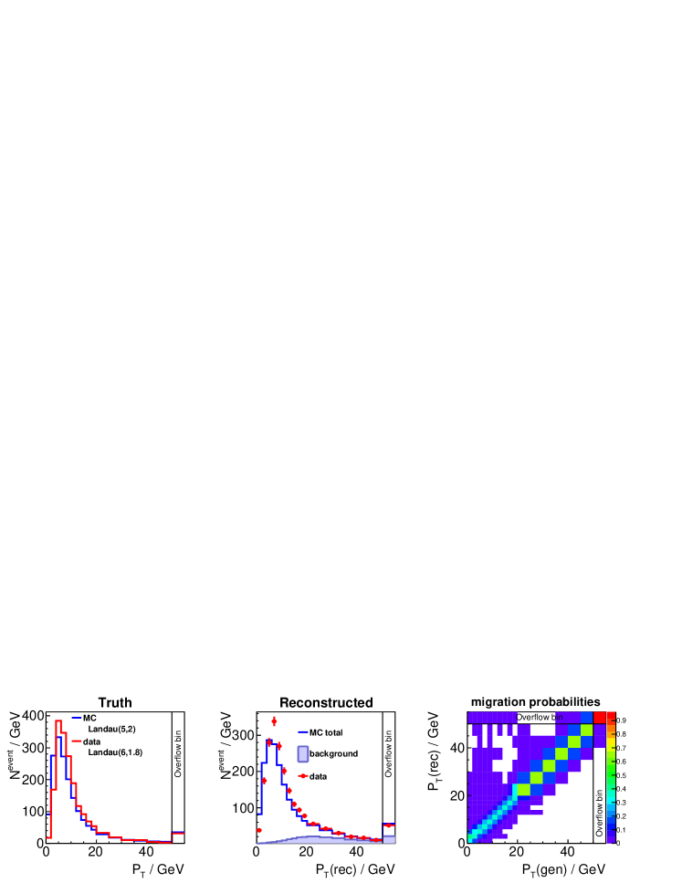
Figure 1: Toy example, distribution on truth level (left), on reconstructed level (middle), response matrix (right).

A heavy particle is produced with a given transverse momentum $P_{T}$ distribution and decays into two massless particles. The energy and angles of the decay products in the laboratory frame are smeared by resolution functions. The observed $P_{T}$ is calculated from the vector sum of the two reconstructed particles. Background is also generated and contributes in this example mainly at large $P_{T}$. For the $P_{T}$ distribution on truth level, Landau distributions are used. The corresponding parameters differ between the “data” and the “simulated” events, where the latter are used to construct the response matrix. The resulting $P_{T}$ distributions are shown in Fig. 1 on truth and detector level. The differences between the two parameterisations are clearly visible, both on truth and on reconstructed level. The response matrix indicates a moderate detector resolution at low $P_{T}$, where a fine binning is used.

3 Testing unfolding results

Given a method to estimate ${\boldsymbol{\hat{x}}}$ and the covariance ${\boldsymbol{V_{xx}}}$ for a given vector of observations ${\boldsymbol{y}}$, it is desirable to judge on the quality of this estimator. Two classes of tests are defined here, “Data tests” and “Closure tests”.

3.1 Data tests

The folding equation 3 can be applied to the unfolding result, i.e. one may compare ${\boldsymbol{A}}{\boldsymbol{\hat{x}}}+{\boldsymbol{b}}$ with the observation ${\boldsymbol{y}}$. The most basic comparison is to verify the normalisation by calculating

$$Y_{\text{unf}}:=\sum_{i=1}^{M}\left({\boldsymbol{A}}{\boldsymbol{\hat{x}}}+{\boldsymbol{b}}\right)_{i}\quad \quad Y_{\text{data}}:=\sum_{i=1}^{M}y_{i}\,.$$ and (6)

The expectation is to find $Y_{\text{unf}}=Y_{\text{data}}$. Another test is to calculate a $\chi^{2}$ sum,

$$\chi^{2}_{A}=({\boldsymbol{A}}{\boldsymbol{\hat{x}}}+{\boldsymbol{b}}-{\boldsymbol{y}})^{\text{T}}({\boldsymbol{V_{yy}}})^{-1}({\boldsymbol{A}}{\boldsymbol{\hat{x}}}+{\boldsymbol{b}}-{\boldsymbol{y}})\,.$$ (7)

In the large sample limit, one expects to find $\chi^{2}_{A}$ distributed with $M_{y}-M_{x}$ degrees of freedom, unless a strong level of regularisation is introduced by the unfolding procedure. In particular, for the case $M_{y}=M_{x}$, the $\chi^{2}$ sum is expected to be zero and hence $Y_{\text{unf}}=Y_{\text{data}}$. For $M_{y}>M_{x}$, the quantiles of the $\chi^{2}$ distribution for $M_{y}-M_{x}$ degrees of freedom can be assessed. Another interesting quantity to study is the average global correlation coefficient,

$$\rho_{\text{avg}} = \frac{1}{M_{x}}\sum_{j=1}^{M_{x}}\rho_{j}\,.$$ (8)

The average global correlation coefficient can be used to tune regularisation parameters, as discussed below. In general, one expects to find a non-zero global correlation coefficient in the presence of non-negligible migrations.

3.2 Closure tests

When using pseudo-data, generated with the help of Monte Carlo simulations, the truth distribution ${\boldsymbol{x^{\text{truth}}}}$ is known, so the unfolding result ${\boldsymbol{\hat{x}}}$ may be directly compared to it. Such comparisons, where pseudo-data are unfolded and compared to the truth are often called closure tests.

The most trivial test to think of is to insert ${\boldsymbol{\mu^{\text{truth}}}}={\boldsymbol{A}}{\boldsymbol{x^{\text{truth}}}}+{\boldsymbol{b}}$ for the observations ${\boldsymbol{y}}$ and perform the unfolding. However, this test is not very meaningful, because basically all commonly used unfolding methods will trivially result in ${\boldsymbol{\hat{x}}}={\boldsymbol{x^{\text{truth}}}}$ in this case.

More interesting closure tests are based on independent Monte Carlo samples. For example, the $y_{i}$ could be drawn from Poisson distributions given the parameters $\mu^{\text{truth}}_{i}$. As these Poisson experiments and the subsequent unfolding are repeated many times, one gets an independent determination of the average and of the covariance

$${\boldsymbol{x^{\text{avg}}}}=\langle{\boldsymbol{\hat{x}}}\rangle, ({\boldsymbol{V_{xx}^{\text{avg}}}})_{jk}=\langle(\hat{x}_{j}-x_{j}^{\text{avg}})(\hat{x}_{k}-x_{k}^{\text{avg}})\rangle\,,$$ and (9)

where the averages are taken over the unfolded, independent Monte Carlo samples. The resulting ${\boldsymbol{x^{\text{avg}}}}$ is expected to agree with ${\boldsymbol{x^{\text{truth}}}}$ and the resulting covariance is expected to agree with the covariance returned by the unfolding algorithm. This type of test, seeded from the same truth distribution as is used to construct the matrix ${\boldsymbol{A}}$ verifies the statistical properties of the unfolding method.

The most interesting type of tests includes independent Monte Carlo samples where the underlying truth distributions are modified. For a good unfolding algorithm, one expects to obtain unbiased results when unfolding observations drawn from the changed truth distribution using the unchanged response matrix. For each of the independent Monte Carlo samples one can define the $\chi^{2}$

$$\chi^{2}_{\text{truth}}=({\boldsymbol{\hat{x}}}-{\boldsymbol{x^{\text{truth}}}})^{\text{T}}{\boldsymbol{V_{xx}}}^{-1}({\boldsymbol{\hat{x}}}-{\boldsymbol{x^{\text{truth}}}})\,.$$ (10)

and verify that the unfolding result is not biased. In the large sample limit and for a completely unbiased algorithm, the quantity $\chi^{2}_{\text{truth}}$ is expected to follow a $\chi^{2}$ distribution with $M_{x}$ degrees of freedom.

4 Unfolding algorithms

4.1 Bin-by-bin correction factors

For this method, the unfolded distribution is given by

$$\hat{x}_{i} = (y_{i}-b_{i})\frac{N_{i}^{\text{gen}}}{N_{i}^{\text{rec}}}\,,$$ (11)

where $N_{i}^{\text{rec}}$ ($N_{i}^{\text{gen}}$) is the total number of reconstructed (generated) Monte Carlo events in bin $i$. This methods is applicable only in the case where $M_{y}=M_{x}$ and where the bins on detector level and truth level have a clear correspondence.

The bin-by-bin method often is used due to its simplicity; however its results are biased significantly by the underlying Monte Carlo distributions. The results of performing data tests using the toy example with various unfolding methods are summarised in Tab. 1. The use of the bin-by-bin method is clearly disfavoured. It yields the wrong normalisation $Y_{\text{unf}}$ and $\chi^{2}_{A}$ is far from zero.

Table 1: Data tests performed on various unfolding methods.

	$Y_{\text{unf}}$	$\chi^{2}_{A}/N_{\text{d.f.}}$	$\mathrm{Prob}(\chi^{2}_{A},N_{\text{d.f.}})$
expectation	$4584$	$N_{\text{d.f.}}$ / $N_{\text{d.f.}}$	$0.5$
bin-by-bin	$4521$	$34.7$ / $0$	n.a.
matrix inversion	$4584$	$0$ / $0$	n.a.
template fit	$4572$	$12.0$ / $16$	$0.74$
constrained template fit	$4584$	$12.0$ / $16$	$0.74$
Tikhonov $\tau=0.0068$	$4584$	$13.4$ / $16$	$0.64$
Tikhonov $\tau=0.012$	$4584$	$15.0$ / $16$	$0.52$
EM method $n=0$	$4537$	$5069$ / $0$	n.a.
EM method $n=20$	$4585$	$5.9$ / $0$	n.a.
EM method $n=100$	$4584$	$4.2$ / $0$	n.a.
EM method $n=1000$	$4584$	$3.9$ / $0$	n.a.
IDS $n=1$	$4584$	$76.8$ / $0$	n.a.
IDS $n=3$	$4584$	$26.1$ / $0$	n.a.
IDS $n=10$	$4584$	$8.0$ / $0$	n.a.
IDS $n=30$	$4584$	$4.9$ / $0$	n.a.

4.2 Matrix inversion and template fit

Another simple unfolding method is based on inverting the matrix ${\boldsymbol{A}}$. This is possible only if the number of bins observed is equal to the number of bins on truth level, $M_{y}=M_{x}$. The unfolded result is given by

$${\boldsymbol{\hat{x}}} = {\boldsymbol{A}}^{-1}({\boldsymbol{y}}-{\boldsymbol{b}})\,.$$ (13)

The matrix inversion returns an unbiased result, because it is a simple linear transformation of the result and no assumptions on the probability distributions of the $y_{i}$ enter the calculation. The result is depicted in Fig. 2. While the folded-back distribution is on spot with the data and all basic tests are fulfilled (Tab. 1), the unfolding result shows large bin-to-bin fluctuations and correspondingly large uncertainties and correlation coefficients close to $-1$ for neighbouring bins. Such “oscillation patterns” are often observed when solving inverse problems. The solution is statistically correct within the uncertainty envelope given by the covariance matrix ${\boldsymbol{V_{xx}}}$.

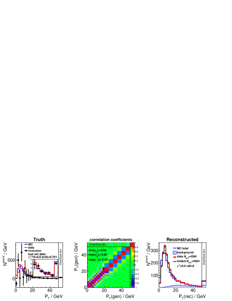
Figure 2: Unfolding result using the matrix inversion method. Shown are the unfolded distribution compared to data and Monte Carlo truth (left), the correlation coefficients (middle) and the unfolded result folded back using the response matrix, compared to Data and Monte Carlo (right).

However, it does not correspond to a smooth curve as expected by the physicist’s prejudice on such a distribution. Extra constraints have to be added to the unfolding procedure in order to enforce such behaviour. These are discussed in the next sections. In the remaining part of this section, template fits are discussed, corresponding to the case $M_{y}>M_{x}$. The template fits are based on a minimisation of the expression $\chi^{2}_{A}$ (equation 7) with respect to the $\hat{x}_{j}$, where the number of degrees of freedom is $M_{y}-M_{x}>0$. Here, $M_{x}=17$ and $M_{y}=33$ are chosen: for each truth bin two bins are used on detector level. In addition there are overflow bins. Simple template fits lead to well-known biases when applied to Poisson-distributed data, such that the overall normalisation is not retained. For this reason, the template fit is repeated, including a constraint on the overall normalisation tunfold . The results of the template fits with and without this constraint are included in Tab. 1. As compared to the matrix inversion, the template fits have somewhat reduced uncertainties and correlations, however the large bin-to-bin fluctuations of the result are still present (not shown in this paper). As summarised in Tab. 1, the template fits pass the data tests with the exception of the overall normalisation for the template fit without constraint, which is slightly low.

4.3 Template fit with Tikhonov regularisation

For the constrained template fit explained above, the large bin-to-bin fluctuations of the result can be reduced by adding an extra term to the $\chi^{2}_{A}$ function (Eq. 7), as suggested by Tikhonov tikhonov . The function which is minimised takes the form

$$\chi^{2}_{\text{TUnfold}}=\chi^{2}_{A}+\tau^{2}\chi^{2}_{L}, \chi^{2}_{L}=({\boldsymbol{\hat{x}}}-{\boldsymbol{x_{B}}})^{\text{T}}{\boldsymbol{L}}^{\text{T}}{\boldsymbol{L}}({\boldsymbol{\hat{x}}}-{\boldsymbol{x_{B}}})\,.$$ where (14)

The vector ${\boldsymbol{x_{B}}}$ is the bias vector, often set to zero or to the Monte Carlo truth. The matrix ${\boldsymbol{L}}$ specifies the regularisation conditions and is here set to the unity matrix. The parameter $\tau$ is the regularisation strength. The case $\tau=0$ corresponds to the template fit without regularisation, whereas for very large $\tau$ the result is strongly biased to ${\boldsymbol{x_{B}}}$. Eq. 14 is modified slightly tunfold to account for the normalisation constraint.

Fig. 3 shows the unfolding result obtained for the choice $\tau=0.0068$. As compared to the matrix inversion, the oscillating behaviour of ${\boldsymbol{\hat{x}}}$ is removed and the uncertainties and correlations are reduced. As compared to Fig. 2, the original of the input distribution is visualized much better.

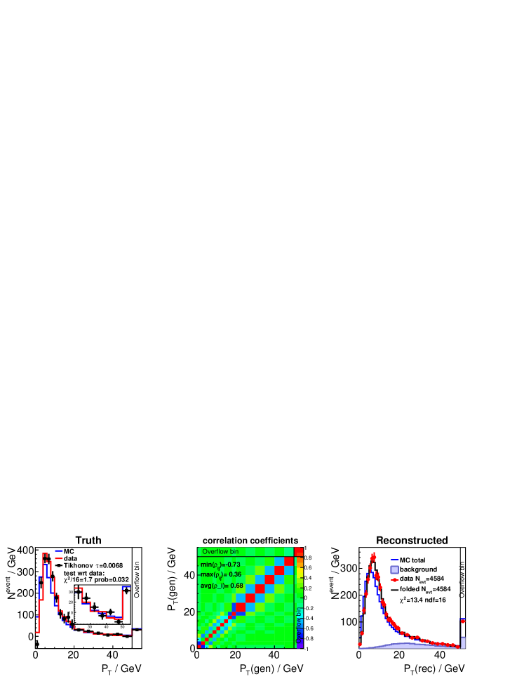
Figure 3: Unfolding result using the constrained template fit with Tikhonov regularisation and parameter $\tau=0.0068$. Further details are given in Fig. 2 caption.

4.4 Choosing regularisation parameters

When using Tikhonov regularisation one has the difficulty to find an appropriate choice of the parameter $\tau$. Similarly, the maximum number of iterations has to be chosen in the case of iterative methods, see section 4.5. Two methods are discussed in the following, the L-curve scan, applicable for the Tikhonov case, and the minimisation of the average global correlation coefficient, which is applicable to a larger class of unfolding methods.

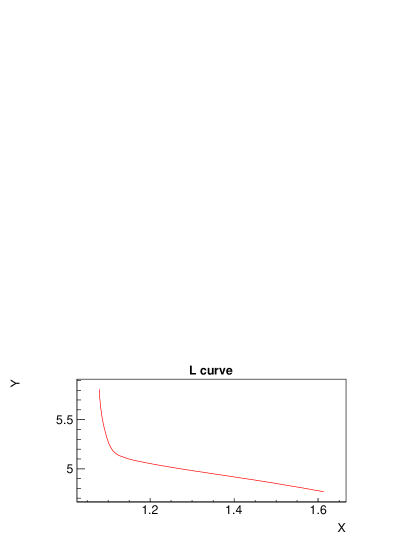
Figure 4: Parametric plot of $X=\log\chi^{2}_{A}$ and $Y=\log\chi^{2}_{L}$ (L-curve).

The L-curve scan is based on investigating the variables $X:=\log\chi^{2}_{A}$ and $Y:=\log\chi^{2}_{L}$. The L-curve is determined by varying $\tau$ and minimising $\chi^{2}_{\text{TUnfold}}$ for each choice of $\tau$. The variables $X$ and $Y$ are visualised on a parametric plot, as shown in Fig. 4. There is a characteristic kink, i.e. the curve is shaped similar to the letter “L”. The kink corresponds to the point with the largest geometric curvature. The corresponding value of $\tau$ is chosen to set the regularisation strength. For a review of the L-curve method, see e.g. hansen2000 .

The minimisation of the average global correlation coefficient globalcorr is also based on repeating the unfolding algorithm for different choices of the regularisation parameter. The average global correlation coefficient (Eq. 8) is recorded and the regularisation parameter is chosen at the minimum $\rho_{\text{avg}}$. The maximisation of the L-curve curvature and the minimisation of $\rho_{\text{avg}}$ as a function of $\tau$ are compared in Fig. 5. In this example, but also in many other cases, the $\rho_{\text{avg}}$ minimisation yields a stronger regularisation than the L-curve method. Both methods pass the test against data, as shown in Tab. 1.

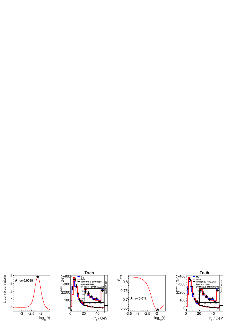
Figure 5: Results of two scans of the parameter $\tau$: L-curve curvature scan (left panels) and scan of average global correlation coefficients (right panels). The scans and the corresponding unfolding result at the final choice of $\tau$ are shown.

4.5 Iterative unfolding methods

Iterative unfolding methods have been proposed since long. Here, two such unfolding methods have been tried: the EM algorithm sheppvardi and the IDS algorithm Malaescu:2009dm . The EM algorithm, in the form described in D'Agostini:1994zf defines an iterative improvement of the unfolding result $x_{i}^{(n+1)}$, given the result of a previous iteration, $x_{j}^{(n)}$,

$$x_{j}^{(n+1)}=x_{j}^{(n)}\sum_{i=1}^{M}\frac{A_{ij}}{\epsilon_{j}}\frac{y_{i}}{\sum_{k=1}^{N}A_{ik}x_{k}^{(n)}}\,.$$ (15)

In the original works sheppvardi ; Kondor:1982ah ; Multhei:1986ps , the efficiency $\epsilon_{j}$ is absorbed in a redefinition $\epsilon_{j}x_{j}\to\tilde{x}_{j}$ and $A_{ij}/\epsilon_{j}\to\tilde{A}_{ij}$, such that $\tilde{x}_{j}^{(n+1)}=\tilde{x}_{j}^{(n)}\sum_{i}\tilde{A}_{ij}y_{i}/\sum_{k}\tilde{A}_{ik}\tilde{x}_{k}^{(n)}$.

The EM algorithm has two interesting properties: given that the start values $x_{j}^{(-1)}$ and the measurements $y_{i}$ are all positive, the result is bound to be positive. Furthermore, it converges to a maximum of the likelihood function, the likelihood defined for the case where the measurements $y_{i}$ are independent and follow Poisson distributions sheppvardi . However, the convergence rate can be very slow and the number of iterations is expected to grow with the number of bins squared Multhei:1986ps . While the method is expected to give unbiased results for a sufficiently large number of iterations with Poisson distributed measurements, this is not necessarily true in other cases, e.g. for correlated input data. This is evident from the fact that the covariance of the input data ${\boldsymbol{V_{yy}}}$ does not enter Eq. 15.

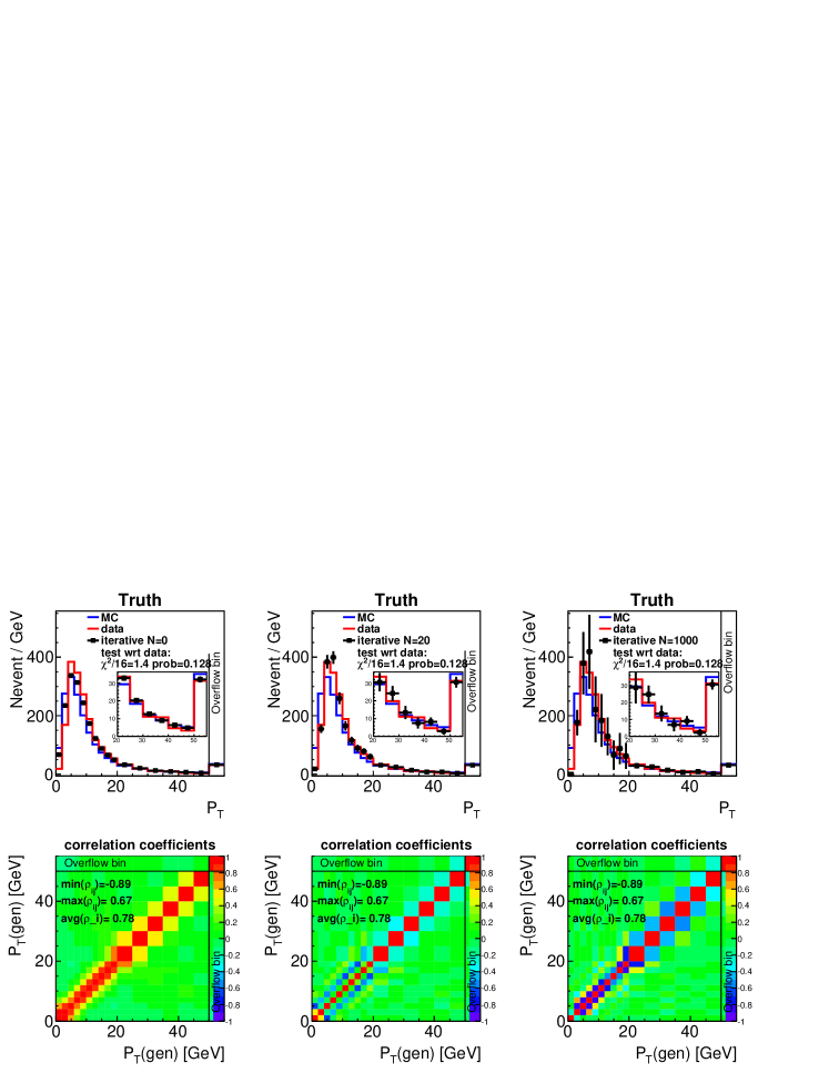
Figure 6: Unfolding results using the iterative EM algorithm. Shown are the results for a number of iterations $n=0$ (left), $n=20$ (middle) and $n=1000$ (right).

In high-energy physics, the EM method typically is not iterated until it converges. Instead, the number of iterations is fixed, and the result then still depends on the start values $x_{j}^{(-1)}$. The dependence on the start values, typically taken to be the Monte Carlo truth, provides a regularisation of the result. Although the algorithm is expected to perform best for $M_{y}>M_{x}$, in high-energy physics often the same number of bins is used on detector and truth level, $M_{y}=M_{x}$. The choice $M_{y}=M_{x}$ is also employed here. For the case of an infinite number of iterations, the EM method with $M_{y}=M_{x}$ is expected to agree with the results of the matrix inversion in those cases where the $\hat{x}_{j}$ obtained by the matrix inversion are all positive.

Eq. 15 has the disadvantage that background is not included. Subtracting the background ${\boldsymbol{b}}$ from ${\boldsymbol{y}}$ in the enumerator is not favourable, because it possibly spoils the positiveness property. For this study, the denominator is modified as follows to take into account the background,

$$x_{j}^{(n+1)} = x_{j}^{(n)}\sum_{i=1}^{M}\frac{A_{ij}}{\epsilon_{j}}\frac{y_{i}}{\sum_{k=1}^{N}A_{ik}x_{k}^{(n)}+b_{i}}.$$ (16)

The results obtained with the EM method for $n=\{0,20,1000\}$ iterations are shown in Fig. 6 and the data tests are summarised in Tab. 1 for $n=\{0,20,100,1000\}$. The results obtained for $n=0$ iterations, corresponding to the non-iterated, so-called Bayesian unfolding D'Agostini:1994zf are very poor, as visible from both the the data tests and from Fig. 6. All bins have positive correlations, corresponding to a smearing rather than unfolding, and the result is far from the truth distribution. The data tests obtained for a low number of iterations indicate that a certain minimum number of iterations is required to reach a proper normalisation. The shapes of the unfolded results observed for $n=20$ and $n=1000$ iterations (Fig. 6) are similar to the cases of Tikhonov regularisation and matrix inversion, respectively.

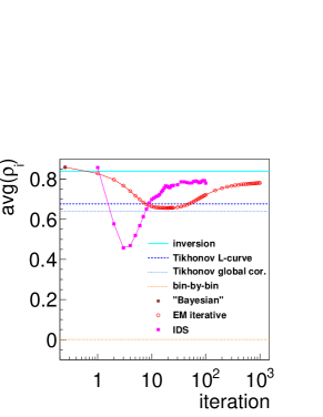
Figure 7: Average global correlation coefficient as a function of the number of iterations.

Another iterative algorithm tested here is the Iterative Dynamically Stabilised unfolding (IDS) Malaescu:2009dm . The algorithm is too complex to be explained here in detail. Briefly, it combines elements of the EM iterative procedure and the bin-by-bin unfolding, using non-linear weighting factors in each bin. For each iteration, care is taken to preserve the data normalisation. Because of the bin-by-bin component in the algorithm, its use is restricted to the case $M_{y}=M_{x}$ or to cases where a clear correspondence of bins on detector and truth level exists Malaescu:2009dm . The IDS algorithm is expected ultimately to converge to the same value as the EM algorithm, however at improved convergence speed Malaescu:private . Results of data comparisons after $n=\{1,3,10,30\}$ iterations are given in Tab. 1. In contrast to the EM method, in this case the data normalisation is correctly reproduced even after only one iteration. The observed $\chi^{2}_{A}$ indicates that a sufficiently large number of iterations is required to accurately match the shapes on detector level.

Table 2: Comparison of selected unfolding results to the “data” truth. When calculating $\chi^{2}_{\text{truth}}$, the overflow bin is not included. The row labelled $\mathrm{Prob}$ corresponds to the quantile of the $\chi^{2}$ distribution for $16$ degrees for freedom.

	$\chi^{2}_{\text{truth}}/N_{\text{d.f.}}$	$\mathrm{Prob}$	$\sigma_{\text{Landau}}$
MC truth	n.a.	n.a.	$2.00\phantom{{}\pm 0.00}$
data truth	n.a.	n.a.	$1.80\phantom{{}\pm 0.00}$
bin-by-bin	$67.8$ / $16$	$0.00$	$2.05\pm 0.05$
matrix inversion	$12.6$ / $16$	$0.70$	$1.80\pm 0.06$
constrained template fit	$13.0$ / $16$	$0.68$	$1.80\pm 0.06$
Tikhonov $\tau=0.0068$	$28.0$ / $16$	$0.03$	$1.86\pm 0.06$
Tikhonov $\tau=0.012$	$100.8$ / $16$	$0.00$	$1.97\pm 0.05$
EM method $n=0$	$4537$ / $16$	$0.00$	$2.24\pm 0.02$
EM method $n=20$	$17.9$ / $16$	$0.33$	$1.91\pm 0.07$
EM method $n=100$	$17.3$ / $16$	$0.37$	$1.77\pm 0.06$
EM method $n=1000$	$22.5$ / $16$	$0.13$	$1.75\pm 0.06$
IDS $n=1$	$4573$ / $16$	$0.00$	$2.30\pm 0.02$
IDS $n=3$	$158.0$ / $16$	$0.00$	$2.27\pm 0.03$
IDS $n=10$	$20.7$ / $16$	$0.19$	$1.97\pm 0.04$
IDS $n=30$	$13.4$ / $16$	$0.64$	$1.81\pm 0.06$

4.6 Scan of average global correlations for iterative methods

The dependence of the average global correlation coefficient and of $\chi^{2}_{\text{truth}}/N_{D.F.}$ on the number of iterations is studied in Fig. 7 for the EM and the IDS algorithms. For both algorithms, a characteristic minimum of $\rho_{\text{avg}}$ is observed. This is related to the fact that the first iteration produces positively correlated results (smearing), whereas in the limit of many iterations (matrix inversion), negative correlation coefficients $\rho_{ij}$ appear. The minimum $\rho_{\text{avg}}$ is interesting to study, because it is largely independent of the start values and hence can be used as an objective to define the number of iterations. The IDS algorithm is observed to converge faster than the EM algorithm. The minimum in $\rho_{\text{avg}}$ is reached after $3$ ($20$) iterations for the IDS (EM) method. The minimum value of $\rho_{\text{avg}}$ determined for the EM method is similar to the minimum observed in template fits with Tikhonov regularisation, whereas the IDS minimum is significantly lower. Most probably this is related to the fact that the IDS algorithm has a bin-by-bin correction component (bin-by-bin trivially results in $\rho_{\text{avg}}=0$).

4.7 Comparisons on truth level

To assess the quality of the unfolding in greater detail, closure tests are performed. The unfolded data are compared to the data truth, which is known for the toy example. In addition, fits of the original Landau function are performed to the unfolded distributions. The comparisons to truth are summarised in Tab. 2. Here, the comparisons are based on unfolding the “data” and comparing to the truth. For more detailed tests, toy studies using the “data” truth would have to be performed in order to assess the quality of the expectation values $\langle\hat{x}\rangle$ and the distribution of $\chi^{2}_{\text{truth}}$.

The bin-by-bin method, the Tikhonov method with large $\tau$ and the iterative methods with small number of iterations all result in unacceptable biases of the extracted width $\sigma_{\text{Landau}}$. As expected, the matrix inversion and constrained template fit results are not biased. The Tikhonov method with L-curve scan, resulting $\tau=0.0068$, gives acceptable results. The EM method works well for a sufficiently large number of iterations, $n\gtrsim 20$, where $n=20$ was determined in the scan of $\rho_{\text{avg}}$. The IDS method also performs well for a sufficiently large number of iterations $n$; however $n=3$ determined in the scan of $\rho_{\text{avg}}$ does not give a satisfactory result.

5 Summary and Conclusions

A selection of methods to unfold binned distributions is studied: bin-by-bin correction factors, matrix inversion, template fits with Tikhonov regularisation, iterative methods. The bin-by-bin methods leads to biased results and should not be used. Matrix inversion and constrained template fits give unbiased results. However, the result typically suffer from large bin-to-bin correlations, large uncertainties and bin-to-bin oscillation patterns.

The oscillations are reduced in the other unfolding methods using regularisation techniques. These damp the fluctuations and reduce bin-to-bin correlations, at the cost of introducing biases. There are free parameters which have to be tuned to obtain a good compromise between bias and damping.

Template fits with Tikhonov regularisation seem to give good results when choosing the regularisation parameter by means of the L-curve method. For the iterative EM method, an interesting choice is the minimisation of the average global correlation coefficients. The IDS iterative method also has been tested but seems to require a different objective to optimise the number of iterations.

In general, methods with Tikhonov regularisation have the advantage, that there is a natural transition to unbiased results, by setting the $\tau$ parameter to zero. In contrast, the iterative methods start from a fully biased results and the number of iterations required to reach the unbiased result is a priory unknown. Furthermore, in the case of bin-to-bin correlated or non-Poisson distributed measurements, it is not clear whether the iterative methods converge to an unbiased estimator.

In summary, no matter which unfolding method is used, detailed closure tests are required to quantify the level of bias introduced by the unfolding.

References

- (1) PHYSTAT 2011 Workshop proceedings, Eds. L. Lyons and H. Prosper, CERN-2011-006.
- (2) J. Kaipio and E. Somersalo, J. Comp. and Appl. Math. 198 (2007), 493.
- (3) P. C. Hansen, Discrete Inverse Problems â Insight and Algorithms, SIAM, Philadelphia, 2010, ISBN 78-0-89871-696-2.
- (4) S. Schmitt, JINST 7 (2012) T10003 [arXiv:1205.6201]; code available at http://www.desy.de/~sschmitt, version 17.6.
- (5) A. N. Tikhonov, Soviet Math. Dokl. 4 (1963), 1035.
- (6) P. C. Hansen, The L-curve and Its Use in the Numerical Treatment of Inverse Problems, Computational Inverse Problems in Electrocardiology, ed. P. Johnston (2000).
- (7) V. Blobel, “Data unfolding”, talk given at the Terascale statistics School, Hamburg (2010) http://www.desy.de/~blobel/.
- (8) L. A. Shepp and Y. Vardi, IEEE Trans. Med. Imaging MI-1 (1982) 113.
- (9) A. Kondor, Nucl. Instrum. Meth. 216 (1983) 177.
- (10) H. N. Mülthei and B. Schorr, Nucl. Instrum. Meth. A 257 (1987) 371.
- (11) G. D’Agostini, Nucl. Instrum. Meth. A 362, 487 (1995).
- (12) B. Malaescu, arXiv:0907.3791; C++ code provided by the author, August 2016.
- (13) B. Malaescu, private communication, August 2016.