An Extension of Chubanov’s Polynomial-Time Linear Programming Algorithm to Second-Order Cone Programming
Tomonari Kitahara
Tokyo Institute of Technology
(Email: kitahara.t.ab@m.titech.ac.jp).Takashi Tsuchiya
National Graduate Institute for Policy Studies
(Email: tsuchiya@grips.ac.jp).
(November 2016
(Revised: December 2016, January 2017))
Abstract
Recently, Chubanov proposed an interesting new polynomial-time algorithm for linear program.
In this paper, we extend his algorithm to second-order cone programming.
Key words:
Chubanov’s algorithm, Linear programming, Second-order cone programming
1 Introduction
In linear programming,
the ellipsoid method [8, 9] and the interior-point method [7, 13] were
the only two algorithms which enjoy polynomiality for a long time.
Recently, an interesting new polynomial-time algorithm was proposed by Chubanov [3, 4, 5].
Related studies include, for instance, [2, 10, 15, 16].
In this paper, we develop a word-by-word extension of Chubanov’s algorithm to second-order cone
programming [1, 6, 12, 13, 14, 17]. Among the related works, Peña and Soheili [15]
developed a polynomial-time projection and rescaling algorithm for a symmetric cone feasibility problem.
Their algorithm utilizes Chubanov’s idea and is closely related to ours in its direction.
We briefly compare the two approaches later to highlight the difference.
Consider the following homogeneous second-order cone programming feasibility problem (P):
where for each and is either a half-line or a second-order cone, i.e.,
We assume that vectors are in column form by default and the vertical concatenation of two vectors and is written as .
We denote by and the set of indices where is a second-order cone and
a half-line, respectively.
The dual problem (D) is
Throughout this paper we use a notation analogous to concerning a second-order cone. When we deal with
a vector in a space where a second-order cone is defined,
the first element with “the index 0” always represents the center axis of a second-order cone, and the second element with the
“index 1” represents the rotational part, unless otherwise stated.
In the following, for a cone , say, we use the notations and to mean that and
, respectively.
Letting , , (P) and (D) are written as
where , , and .
For simplicity, we assume that is row independent.
By generalized Gordan’s theorem, (P) has an interior feasible solution if and only if
(D) does not have a nonzero solution (i.e., zero is the only solution to (D)), and
(D) has an interior feasible solution if and only if
(P) does not have a nonzero solution. If we let
the Generalized Gordan’s Theorem says that (GP) has a solution if and only if (GD) does not have a solution
and (GD) has a solution if and only if (GP) does not have a solution.
Given a matrix , say, let be an orthogonal projection matrix to . If is a row independent
matrix, . The problem (P) is written as
and the problem (D) is written as
(where “the free variable” is eliminated).
We will develop a polynomial-time algorithm for finding a solution to (GP) or (GD) or detecting
no -interior feasible solution exists to (P) (the definition of
-interior feasible solution is given below).
In Appendix we describe how we can solve approximately
a general second-order cone program with a primal-dual interior feasible solution by the algorithm
developed in this paper.
The problem (P) is equivalent to finding an interior feasible solution to the following system.
We denote by the set of feasible solutions to this system.
We define the projection of onto the block as follows:
(1)
For a point , its minimum eigenvalue
is defined as
A point is called an -interior point of if .
We define the maximum eigenvalue as
If , then
the following equivalence relation holds betweens and :
(2)
For , the following quantity is called the determinant of :
The determinant of is defined as:
Let , where
Here denotes the dimensional zero vector and we use analogous notation onwards.
We have the following proposition.
Proposition 1.1
Let . The following relations hold:
1.
2.
Let .
A point is called an -interior-feasible solution to (P) if the following condition is satisfied:
We develop a polynomial-time algorithm to find an interior feasible solution to (P) or a
nonzero feasible solution to (D),
or conclude that no -interior feasible solution exists to (P). The algorithm terminates in
iterations of a procedure called a basic procedure.
The basic procedure requires
arithmetic operations (assuming that the standard linear algebraic procedures are employed).
Therefore, the algorithm terminates in
)
arithmetic operataions.
The basic procedure is a heart of Chubanov’s algorithm.
In the following, we explain our algorithm in comparison with Chubanov’s original algorithm, and discuss the difference between our algorithm
and Peña and Soheili’s algorithm.
Chubanov’s algorithm is to find a point in the intersection of a linear space and a unit hypercube,
i.e., the direct product of 0-1 segments. For simplicity, we assume that the system is interior feasible.
The algorithm first performs the basic procedure.
The basic procedure either (i) finds an interior feasible solution, or (ii) detects a variable whose value cannot be greater than 1/2
in the feasible region. Detection is done by finding a “cut”, a hyperplane to cut off the region where no feasible solution exists.
Once such “cut” is found, then the associated coordinate is rescaled by a factor of two so that the hypercube is recovered,
to continue the same procedure.
In terms of the original
coordinate, this process is regarded as
generating a series of shrinking convex bodies of the same type, i.e., a hyper-rectangle, which enclose feasible solutions.
Now we illustrate our algorithm. For the ease of understanding, we assume that is just a single second-order cone
and that there exists an interior feasible solution. We let .
Let be the intersection of the feasible solution to (P) and , which we call “the standard truncated second-order cone.”
The algorithm is to find an interior feasible solution in . To this end,
first we perform the basic procedure. The basic procedure either (i) finds an interior solution to (P), or (ii) finds a hyperplane called a “cut” . The cut defines an obliquely truncated second-order cone .
This cut is a natural extension of the one by Chubanov, and is one of the key ideas of this paper.
In virtue of the basic procedure, the set contains and has smaller volume than at least by a constant factor.
Thus, if a cut is found, we can shrink the region where the feasible solutions exist.
Then, is transformed to with an automorphism transformation of the cone .
We apply the same procedure to the transformed problem, and repeat it over and over.
This way, the algorithm constructs a series of shrinking obliquely truncated second-order cone which contains
a nonzero feasible solution to (P).
It is shown that the volume of obliquely truncated second-order cone converges linearly to zero. Therefore,
if there exists an interior feasible solution, then shrinkage cannot last forever and the algorithm and the basic procedure
ends with (i) at a certain point.
This is a rough sketch of the algorithm, and the idea will be generalized to the multiple cone case in the rest of this paper.
Interestingly, while the new algorithm has similarity to the ellipsoid method in the sense that it generates
a series of shrinking convex bodies of the same type, it has some flavor of the interior-point method in that
it utilizes the automorphism group of the cone.
The idea of the cut and the basic procedure is two key concepts in Chubanov’s algorithm, and will be extended to the second-order
cone programming case in this paper.
As is readily seen from the above explanations of the two algorithms,
our algorithm is a word-by-word generalization of Chubanov’s algortihm.
Peña and Soheili [15] developed a polynomial-time projection and rescaling algorithm for the symmetric cone feasibility problem.
Their algorithm consists of rescaling step and the basic procedure to find a vector for rescaling, where rescaling procedure is
inspired by Chubanov’s idea.
They measure the progress of the algorithm with a condition number of the system which is essentially the determinant.
The condition number is bounded above by one, and the system whose condition number is closer to one is better conditioned. In their algorithm,
the condition number is increased by a constant factor at each iteration by rescaling, or the algorithm finds an interior feasible
solution. The Chubanov’s cut vector is used as an algebraic machinery to rescale the system properly.
Their algorithm plays with scaling (or metric), but does not change the shape of the region on focus.
This makes a remarkable contrast with our approach as we argue below.
Our algorithm uses the cut to confine the region of existence of the feasible solutions
and generates a series of shrinking convex bodies of the same type containing the feasible region.
In this regard, our algorithm is geometrically intuitive and can be considered as a direct and
word-by-word extension of Chubanov’s algorithm.
In our algorithm, we measure the progress of the algorithm with the volume of the shrinking area of
existence of the feasible solutions, which is essentially the determinant.
Thus, the determinant plays crucial roles in the both algorithms and they share some features in common.
The paper is organized as follows. In Section 2, we introduce the second-order cone and its automorphism group,
and study some basic properties of the truncated second-order cones. In Section 3, we discuss an extension of
Chubanov’s fundamental relation in the context of second-order cone programming.
In Section 4, we extend and analyze the basic procedure.
In Sections 5, we develop the main algorithm.
In Section 6, we make some remarks. Section 7 is a conclusion.
Note added at the Second Revision (January 2017):
We removed “Section 6: Full Version” of the paper,
because we found a flaw in its complexity analysis.
The intension of that section was to reduce the complexity by a factor of from the algorithm
in Section 5 by adapting Chubanov’s
elegant idea [5] of initiating a basic procedure using the second last iterate of the preceding basic procedure.
We realized that the argument we made in the previous version does not work.
We feel very sorry to the readers about this mistake, but we consider that the main part of the paper, development of
an extension of Chubanov’s algorithm to second-order cone program and its polynomial-time complexity analysis, yet
survives.
Note added at the First Revision (December 2016):
1.
We corrected an nontrivial error in evaluating complexity of the basic procedure.
In the first version released in November 2016, we conducted analysis assuming that one iteration of the
basic procedure can be done in arithmetic operations like in the case of linear program.
But later we realized that the argument in the first version was not correct and
that one iteration of the basic procedure requires arithmetic operations.
At Step 5 of the basic procedure, we compute and this requires arithmetic operations.
This affects overall complexity estimate of the entire algorithms. We corrected them accordingly.
We feel very sorry for the confusion caused by this flaw.
2.
We refer the reference [15] and added related considerations in this introduction.
We also updated references and corrected some misleading statements related to [16].
A few (easily fixable) mathematical errors are also corrected.
2 Preliminary Observations
We assume that is a -dimensional second-order cone (). For , we define
i.e., is the half space in whose boundary normal vector is and is on the boundary.
The boundary hyperplane of is written as .
Let .
The intersection of the second-order cone and the half space
is referred to as the standard truncated second-order cone (S-TSOC).
We denote by the volume of -dimensional S-TSOC. Its concrete
formula is:
which is obtained by integrating the volume of -dimensional hypersphere from the radius to 1.
Let and .
Then is a non-empty bounded domain
which is obtained by cutting with a tilted hyperplane. This set is referred to as an obliquely truncated second-order cone (O-TSOC).
We let
With this notation, S-TSOC is written as .
The automorphism group of a cone is the set of linear transformations such that
We denote by the automorphism group of .
Let and be such that .
In the following, we show that there exists an element of which maps
S-TSOC to . This plays an important role throughout our algorithm
development and analysis.
We start with the following statement.
Proposition 2.1
If satisfies the following conditions:
1.
(3)
2.
There exists a point such that ,
then, , and hence and are elements of .
Proof. We fix and show that if the condition 1 with and
the condition 2 are satisfied, then holds.
This is enough to prove the proposition with general .
The main part of the proof is to show that is invertible and
, where is the boundary of . Once this is shown, readily follows since is a linear transformation. After this, we will proceed to demonstrate that .
We prove that is invertible and .
The condition 1 immediately implies that is an invertible matrix.
Consider the image where
Let and let .
Since and hence holds,we have or . We show that the second case never occurs.
Suppose that there exists a point such that .
Consider the line ,
and let . Then, since , we have
but , yielding that for some .
This implies that as well. However,
since is in the interior of , we have whereas
and hence , which is a clear contradiction
to the condition 1. Thus, whenever , we have .
This shows that . If we take , satisfies the
conditions 1 and 2. Therefore, we have and hence
.
Thus, we have shown .
Since is a linear transformation,
follows immediately.
Now we show that . Let
Multiplying from the left on the both sides of (3) and by using and that is invertible, we
obtain . In order to show , we use the fact that
if and only if . We apply this by choosing .
Since , we have . Then it follows that
. It remains to show that . Since , we have
Since , we have , and we are done.
In the following, we will find such that
Since
it is enough to find an element of the automorphism
group such that , and since , this amounts to finding such that
where
and .
Since ,
We have .
The tangent space of is
and this should be equal to the tangent space of .
Since should hold,
Therefore, we have with (c.f. ).
This implies that and equivalently .
Since , so is
, then we have and hence .
Note that is an element of which maps to
. Since , we have . Substituting
into this formula, we obtain that .
In summary, if and ,
should satisfy . On the other hand, if we can find satisfying
this condition, we have .
In the following, we find satisfying the condition .
Let , , where ,
and let
It is not difficult to check that satisfies the conditions 1 and 2 in Proposition 2.1,
being a member of .
In particular, we see that and .
Hence we have .
Since ,
we let and obtain
By direct calculation it is easy to confirm that
Therefore, we have
(4)
and
(5)
Thus, we obtain the following proposition.
Proposition 2.2
Let , , and
consider O-TSOC .
Then the matrix
where
maps S-TSOC to , i.e.,
and
Suppose that is given, and that we want to find which minimizes the volume of
. Since , without loss of generality, we may assume that satisfies
. Furthermore,
due to rotational symmetry with respect to the 0th axis,
we assume that, without loss of generality, .
In order to minimize , we just minimize
Solving this problem, we obtain that
where .
and the optimal value is:
This consideration is summarized as the following proposition:
Proposition 2.3
Let .
A normal vector which minimizes the volume
is given as
and
Corollary 2.4
Let . Then, the minimum volume O-TSOC containing is given as
and hence the minimum volume is given as
Proof. Let us denote by an O-TSOC satisfying the condition.
Then we can take , since, otherwise, we can make a parallel
shift of the boundary hyperplane until it touches
after the shift.
Now we can apply the previous lemma to obtain the result.
Proposition 2.5
Let .
If , then
The strict inequality version of this relation also holds.
Proof. The relation obviously holds because
Proposition 2.6
Let and be as defined in Section 1. Let and
, and
suppose that and .
Then, there does not exist an -interior solution in .
Proof. By contradiction, we assume that there exists an -interior solution , say, in .
The -th block of this solution satisfies
because (the contraposition of Proposition 2.5).
Since , is an O-TSOC containing
and therefore, in view of Corollary 2.4,
holds, which is a contradiction to the initial assumption that .
In the end of this section, we introduce a scaling operation of (P) and (D).
Let for , and consider the dual pair of the problems (SP) and (SD):
where for and
(SP) and (SD) are mutually dual and they are obviously equivalent to (P) and (D). Following interior-point terminology,
we call (SP) and (SD) “scaled problems.” In the algorithm developed in this paper, we mostly work with scaled problems
(SP) and (SD). The original problems (P) and (D) appear only in the beginning and in the end
of the algorithm.
3 Basic Lemma and its Consequences
We extend a fundamental relation established by Chubanov (Formula (2), Section 2.1, [5])
and its consequences to the second-order cone case.
For notational convenience, we develop the results in terms of (P) and (D) in Section 1.
Later we will apply the results in this section to scaled problems (SP) and (SD).
It is easy to translate the results written in terms of (P) and (D) into the corresponding results in terms of (SP) and (SD).
In the rest of the paper, we denote
the S-TSOC of the -th block by , i.e., .
The extension of Chubanov’s fundamental relation to the second-order cone case is described as follows.
Lemma 3.1
(Basic Lemma)
Suppose .
Suppose that satisfies the homogeneous inequality
for some index . Then, if is a half-line, we have
and if is a second-order cone, then,
In other words, any feasible solution to (P) satisfies if is a half-line, and
if is a second order cone.
Proof. We give a proof for the case where is a second-order cone. The half-line case is analogous and easy.
We have if and . Therefore,
Thus, we see that any is contained in the half space
We call satisfying the condition of lemma as “a cut generating vector,” and
and are referred to as “generating index” and “generating block,” respectively.
Suppose that , and a cut generating vector with generating index is found.
In the rest of this section,
we construct an O-TSOC which encloses and with smaller volume than
by choosing appropriate and .
Specifically, we find satisfying the following two conditions:
(6)
(7)
If these conditions are satisfied, the pair is called “a cut.”
We also use the term “cut” for the hyperplane .
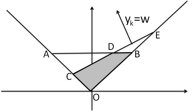
Figure 1: Case 1
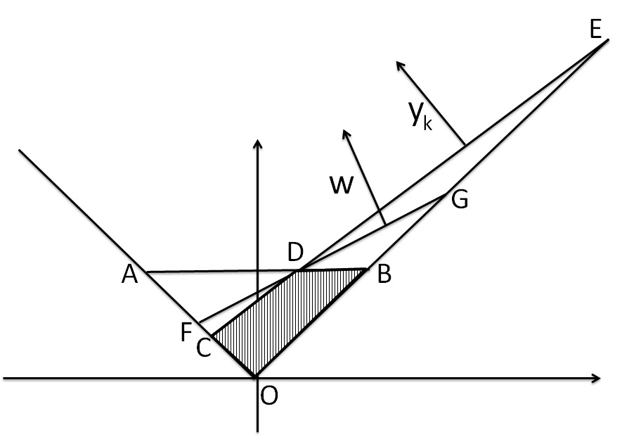
Figure 2: Case 2
We illustrate the situation in Figure 1 for the case where the dimension of is two.
In the beginning, we only know that is enclosed
in the triangle AOB ().
Let a cut generating vector is given with generating index .
The quadrangle COBD, which is the intersection of the two triangles AOB and COE ,
is the reduced area where
is still enclosed. (The triangle ACD is the area which was “cut off.”)
Here, the line CE can be taken as a cut.
Figure 1 intuitively shows that the triangle OCE satisfies the conditions (6) and (7),
since it encloses the quadrangle COBD and the area of the triangle COE is smaller than the triangle AOB
Now we generalize this intuitive observation in a more quantitative manner to construct an O-TSOC we are aiming at.
We branch into two cases: (Case 1) The angle between and the center axis is small;
(Case 2) The angle between and is large.
(Analysis of Case 1)
In general, since ,
we can take, as was suggested in the above,
and . This means that we just use
as a confined enclosing area for satisfying (6) and (7).
The volume of is, by letting in Proposition2.3, given as
If , the volume is ensured to decrease.
For later convenience, let . We have , and let .
Since and so is , the range of is .
In terms of , the condition is written equivalently as .
Under this condition, the reduction ratio of the volume is written as:
Observe that this is a monotonically increasing function.
The above idea does not work for .
See Figure 2. Observe that is almost parallel to the edge of the cone.
The vertex is seen further than before.
The quadrangle COBD contains .
The triangle COE is larger than the original triangle AOB though it contains
the quadrangle COBD. The triangle COE cannot be used to confine the existing area of this time.
We consider the following approach to deal with this case.
We continue explanation with Figure 2. This time,
we generate a supporting line (segment) FG which touches the quadrangle COBD at the vertex D, and enclose
the quadrangle COBD with the triangle FOG. The line FG is chosen so that the triangle FOG contains the quadrangle COBD and
its volume gets smaller than the original triangle AOB.
We already developed a formula to find a line which goes through and minimizes the area of the triangle FOG,
see Proposition 2.4. We also need to check that the resulting line does not intersect the quadrangle
COBD.
(Analysis of Case 2)
Consider a half-space which contains such that
its boundary is a supporting hyperplane to
. Obviously, we have
Since is a supporting hyperplane to ,
without loss of generality, we assume that
(8)
Let , then and .
We let as before. We assume that is written as follows
(9)
and try to find and satisfying the condition such that
Then Proposition 2.3 yields that the minimum volume O-TSOC is obtained
by taking
and
Observe that is a monotonically increasing function of whose value is positive in the interval
. It is easy to see that .
Now we examine the condition that defines a supporting hyperplane of .
Since and ,
a necessary and sufficient condition for to be the supporting hyperplane
is that is written as a nonnegative combination of and . Since
,
Thus, is on the line connecting and , and can be represented as
a conic combination of (or equivalently ) and if and only if
, i.e.,
The analysis so far is summarized as follows:
1.
Suppose that . Then, by letting and ,
O-TSOC encloses and its volume is bounded by
The function is well-defined in the interval
and is monotonically increasing. In particular, if , we have
.
2.
Suppose that . Then by letting
O-TSOC encloses and its volume is bounded by
as long as . In particular, is in the
interval.
The function is monotone increasing, and we have
Therefore, given the cut generating vector with generating index , if we determine and according to the
rule that
1.
if , then take and as in the item 1 above,
2.
if , then take and as in the item 2 above.
Then, O-TSOC encloses and
the bound
is ensured. Finally, Proposition 2.2 yields that an element of the automorphism group which maps
to is:
where and .
4 Basic Procedure and its Analysis
In this section, we explain and analyze the basic procedure which is a direct extension of Chubanov’s.
The basic procedure deals with a pair of the dual problems and , and
finds either a primal interior solution, or dual nonzero solution, or a cut generating vector.
In the procedure, the iterate satisfying is updated every iteration.
As will be discussed later, the iteration complexity estimate is based on the fact that
the quantity increases at least by 1/2 at each iteration.
On the other hand, we can show that is a cut generating vector if .
Then, the basic procedure is ensured to terminate in iterations regardless of the choice of
initial value of . Before we proceed, we make two important comments:
1.
The basic procedure is mainly applied
to a scaled system (SP) and (SD). But we describe the procedure and conduct analysis just for (P) and (D) to avoid
that the notation gets too heavy.
2.
In Chubanov’s algorithm, one iteration of his basic procedure requires just arithmetic operations
though it computes projection of a vector to and appears to require arithmetic operations.
In our case, the complexity of one iteration of the basic procedure is a bit higher and arithmetic
operations, because the second-order cone is a bit more complicated than linear inequalities.
We mention that Peña and Soheili [15] extends the basic procedure to general symmetric cone programming.
The Basic Procedure
Input Matrix and vector such that , ,
Output One of the followings :
(i) A cut generating vector and its generating index ,
(ii) Solution to , ; (iii) Solution to ,
Procedure
1.
Compute and .
2.
Check termination conditions (based on ):
(a)
If , then is dual interior feasible. Return “(iii)” and .
(b)
If , then, is primal interior feasible. Return “(ii)” and .
(c)
If holds for some , return “(i)”, and, and as a cut generating vector
and a generating index, respectively.
(d)
If (a)–(c) does not hold, then, go to Step 3.
3.
Since the conditions (a) and (b) do not hold, and .
Therefore, there exists an index , say, such that and hold.
In the following, we construct such that
•
If is a half-line, then, we set . (, are scalers and .)
•
If is a second-order cone,
such is computed as follows.
–
If , then we let ;
–
If
, then, we let
where ().
In this case, holds because . Therefore, we have
4.
Let . Then we have and .
5.
Let . Computation of requires arithmetic operations, since is already computed and contains nonzero elements.
6.
Check termination conditions (based on ):
(a)
If , then is dual feasible. Return “(iii)” and .
(b)
If , then, is primal interior feasible. Return “(ii)” and .
(c)
If neither of (a) nor (b) holds, go to Step 7.
7.
Construct a new iterate as follows:
Note that and are ensured, and that
is chosen so that is closest to the origin. Then it follows that
is positive as is discussed below.
Since and , we have .
Since , .
So we continue iteration by letting , and going to Step 2.
(Analysis of change of )
We show that increases by at least 1/2 per iteration.
Observe that
Furthermore, since
and neither nor is zero, . Therefore, we have .
Letting , we have
Therefore,
Substituting the concrete formula of into the above and using , we obtain
Since is a projection matrix, we have .
This implies that
Complexity Analysis of the Basic Procedure
Now we analyze overall complexity of the basic procedure.
Prior to the iteration of the basic procedure, we compute and . This
requires arithmetic operations.
In one iteration of the basic procedure, we need to compute . This can be done in arithmetic operations as explained in the previous section.
We analyze that the number of iterations of the basic procedure is .
Recall the condition that is a cut generating vector with generating index is .
since and , we obtain that . Therefore, if
then associated with is a cut generating vector.
As we already analyzed, at each step of the basic procedure increases by 1/2. Therefore,
in iterations of the basic procedure, we find a cut generating vector or a primal interior feasible solution or dual nonzero feasible solution. Since one iteration of the basic procedure
requires arithmetic operations, the basic procedure terminates in arithmetic operations.
5 Main Algorithm
We are ready to describe the main algorithm.
This algorithm (i) finds an interior feasible solution to (P),
(ii) finds a nonzero solution to (D), or (iii) concludes that there exists no -interior
feasible solution in iterations of the basic procedure,
where the basic procedure requires arithmetic operations.
Thus, the overall arithmetic operations of the algorithm presented in this section is .
The Main Algorithm
Input A matrix and a cone which is the direct product of second-order cones and half-lines,
Output One of the followings :
(i) Solution to , ; (ii) Solution to ,
(iii) Declare “No -interior solution to , .”
Algorithm
1.
Let , , , , ,
, ;
2.
Call the Basic Procedure (BP) by setting and as Input (See Section 4).
(C1)
If (BP) returns a cut generating vector and generating index ,
then proceed to Step 3.
(C2)
If (BP) returns an interior solution to , then we let
and return as an interior solution to (P).
(C3)
If (BP) returns a nonzero solution to , , then return
as a nonzero solution to (D).
3.
In the case of (C1),
•
if is a half space then set .
•
if is a second-order cone and where , then set , ,
and construct according to Prposition 2.2 as an automorphism transformation of mapping to .
•
if is a second-order cone and where , then set
and construct according to Proposition 2.2 as an automorphism transformation of mapping to .
4.
We set
Regarding other blocks than , we let
5.
If , then, we conlude that there is no interior feasible solution to (P).
Otherwise, we set and return to Step 2.
Overall Complexity Analysis
Now we analyze the complexity of the main algorithm.
In the beginning of the algorithm, is enclosed in for all .
The algorithm terminates
(i) In the middle of the basic procedure by finding an interior solution to (P) or nonzero solution to (D);
(ii) Detecting that there is no -interior feasible solution.
Let be the iteration number in which the -th block is transformed.
Let be the matrix of the automorphism
transformation associated with performed in the course of the algorithm. Then it follows that
So, in view of Proposition 2.4, we conclude (ii) when the following relation holds:
This relation implies that is bounded by .
The most time consuming case is that the number of occurrence of cutting process is almost even
for all cones
before termination of the algorithm.
Then, the number of execution of the basic procedure is bounded by .
Since executions of the basic procedure might be necessary before completion of the whole procedure,
the complexity of the proposed algorithm is .
6 Remarks
Before concluding this paper, we make some remarks.
6.1 Condition Number
We define a condition number of (P) as follows:
If (P) have an interior feasible solution, stays finite, but it becomes infinity if (P) is feasible but
is not interior feasible. This quantity is useful in evaluating the complexity of the main algorithm developed
in this paper. It is worth noting that , where is the optimal
value of the following problem:
6.2 Running Time to Find a Feasible Solution to an Interior-feasible System
Suppose that we set and run the main algorithm.
The algorithm will never stop if (P) does not have an interior feasible solution. But if there exists an
interior feasible solution, then the algorithm is ensured to terminate in execution of
of the basic procedure, where is the optimal value of the following optimization problem:
In view of (2), we have . Therefore, the algorithm is
capable of finding an interior solution to (P) in times execution of the basic procedure.
6.3 SOCP Feasibility Problem
Suppose that we deal with the problem of finding an interior-feasible solution to
(11)
where is a direct product of second-order cones/half-lines.
We assume the system is interior-feasible.
To solve this problem, we consider the homogenized system
where is a half-line.
We run the main algorithm with . The algorithm stops in
iterations.
For any feasible solution to ,
is an upper bound for .
This implies that if the system (11) have an interior feasible
solution whose components are more or less in the same magnitude,
then less number of iterations is required to find an interior feasible solution.
7 Conclusion
We extended Chubanov’s algorithm for linear programming to second-order cone programming.
The extension to semidefinite programming and symmetric cone programming is an interesting
topic for further research.
In the case of linear program, Chubanov [5] developed a technique to reduce the complexity by a factor of by
initiating a basic procedure using the second last iterate of the preceding basic procedure.
This idea does not directly carry over to the second-order cone program. Extending the technique to the second-order cone
program is another interesting subject.
As was mentioned in introduction, Peña and Soheili developed an extension
to Chubanov’s algorithm to symmetric cone programming. We hope that
comparison of our extension and their algorithm will shed new insight into substance of Chubanov’s idea in conic programming.
Acknowledgement
We would like to thank Dr. Bruno F. Lourenço of Seikei University for his careful reading of the first manuscript and suggesting improvement,
and for bringing the reference [15] to our attention.
The aurhors are supported in part with Grant-in-Aid for Scientific Research (B), 2015, 15H02968,
from the Japan Society for the Promotion of Sciences. The first author is supported in part with Grant-in-Aid for Young Scientists (B), 15K15941.
Appendix
In this section, we describe how we can solve a standard SOCP problem with the algorithm developed in this paper.
Consider the pair of primal and dual SOCP:
and
Suppose (P) and (D) have interior feasible solutions. Then
(P) and (D) have optimal solutions with the same optimal value.
Furthermore, the optimal set is bounded for the both problems.
In this appendix,
we explain, given any , how the algorithm developed in this paper can be used to
find a feasible solutions satisfying . If is sufficiently
small, then , and are approximate optimal solutions to (P) and (D).
It is well-known that (P) and (D) are equivalent to the following problem.
We have the following proposition.
Proposition A.1Let and be an interior feasible solution to (P) and (D),
respectively. Let
If ,
has -interior feasible solution.
Proof. is a -interior feasible solution to (PD).
Let , be optimal solutions to (P) and (D), and define
Then, is a -interior feasible solution to (PD) for any .
We also have
It is easy to check that , is indeed -interior feasible solution
to (PD()) for , and we are done.
We may consider , and as a feasible solution obtained in Phase I.
Now we are ready to describe an algorithm to solve (P) and (D) approximately.
The algorithm works in two phases.
1.
(Phase I) We apply the feasibility algorithm described in Section 6.3
to
with .
(This problem contains as a free variable, but
we can apply the main algorithm after rewriting the condition with to eliminate
. In the end of the algorithm, we can recover from .)
Then, we will find an interior feasible solution
.
The complexity of this step is estimated with the result in Section 6.3,
in terms of the condition number. Let
.
Then, is an -interior
feasible solution to (PD).
2.
(Phase II) If we want to reduce the objective value by a factor of from ,
we solve the interior-feasibility problem (PD()) above, which is ensured to have an
-interior feasible solution.
The complexity is estimated with the result in Section 6.3, again, in terms of the condition number of (PD()).
References
[1] F. Alizadeh and D. Goldfarb: Second-order cone programming.
Mathematical programming, Vol.95 (2003), pp.3-51.
[2]
A. Basu, J. A. De Loera, M. Junod: On Chubanov’s method for linear programming.
Informs journal on computing, Vol.26 (2013), pp.336-350.
[3]
S. Chubanov: A polynomial relaxation-type algorithm for linear programming.
Optimization Online, February, 2011.
[4]
S. Chubanov: A strongly polynomial algorithm for linear systems having a binary
solution. Mathematical Programming, Vol.134 (2012), pp.533-570.
[5]
S. Chubanov: A polynomial projection algorithm for linear programming for linear feasibility problems.
Mathematical Programming, Vol.153 (2015), pp.687-713.
[6] F. Cucker, J. Peña and V. Roshchina: Solving second-order conic systems with variable precision.
Mathematical Programming, Vol.150 (2015), pp 217-250.
[7] N. Karmarkar:
A New Polynomial Time Algorithm for Linear Programming. Combinatorica, Vol.4 (1984), pp.373-395.
[8]L. G. Khachiyan: A Polynomial Algorithm in Linear Programming. Doklady
Akademiia Nauk SSSR, Vol.244 (1979), pp.1093-1096 (in Russian, translated in Soviet Mathematics
Doklady, Vol.20 (1979), pp.191-194).
[9]L. G. Khachiyan:
Polynomial Algorithms in Linear Programming. Zhurnal
Vychisditel’noi Matematiki i Matematicheskoi Fiziki, Vol.20 (1980), pp.51-68 (in Russian).
[10]
D. Li, K. Roos, and T. Terlaky:
A polynomial column-wise rescaling von Neumann algorithm. Optimization Onine, June, 2015.
[11] M. S. Lobo, , L. Vandenberghe, S. Boyd, H. Lebret:
Applications of second-order cone programming.
Linear Algebra and its Applications, Vol.284, (1998), pp.193-228.
[12] R. D. C. Monteiro and T. Tsuchiya: Polynomial convergence of primal-dual algorithms for the second-order cone program based on the MZ-family of directions.
Mathematical Programming, Vol.88 (2000), pp.61-83.
[13]
Y. E. Nesterov and A. S. Nemirovskii. Interior point polynomial methods in convex programming:
Theory and Applications, SIAM, Philadelphia, 1994.
[14]Y. E. Nesterov and M. J. Todd: Self-scaled barriers and interior-point methods for convex programming
Mathematics of Operations research, Vol.22, pp.1-42 (1997).
[15] J. Peña and N. Soheili: Solving conic systems via projection and rescaling. arXiv:1512.06154v2[math.OC], April, 2016.
[16] K. Roos: An improved version of Chubanov fs method for solving a homogeneous feasibility problem.
Optimization online, November 2015 (Revised: July 2016).
[17]T. Tsuchiya: A Convergence Analysis of the Scaling-invariant Primal-dual Path-following Algorithms for Second-order Cone Programming. Optimization Methods and Software, Vol.11/12 (1999), pp.141-182.