Semiclassical Asymptotics
of $\mathbf{GL}_{N}({\mathbb{C}})$ Tensor Products
and Quantum Random Matrices

Abstract.

The Littlewood–Richardson process is a discrete random point process arising from the isotypic decomposition of tensor products of irreducible representations of the linear group $\mathrm{GL}_{N}({\mathbb{C}})$. Biane–Perelomov–Popov matrices are quantum random matrices obtained as the geometric quantization of random Hermitian matrices with deterministic eigenvalues and uniformly random eigenvectors. As first observed by Biane, the correlation functions of certain global observables of the LR process coincide with the correlation functions of linear statistics of sums of classically independent BPP matrices, thereby enabling a random matrix approach to the statistical study of $\mathrm{GL}_{N}({\mathbb{C}})$ tensor products. In this paper, we prove an optimal result: classically independent BPP matrices become freely independent in any semiclassical/large-dimension limit. This proves and generalizes a conjecture of Bufetov and Gorin, and leads to a Law of Large Numbers for the BPP observables of the LR process which holds in any and all semiclassical scalings.

To Philippe Biane, for his 55th birthday.

1. Introduction

1.1. The Littlewood–Richardson process

Rational representations of the complex general linear group, $\operatorname{GL}_{N}({\mathbb{C}})$, were classified by Schur more than a century ago, see e.g. Weyl’s classic book [Wey97]. This classification may be stated as follows: irreducible representations are parametrized, up to isomorphsim, by configurations of $N$ hard particles on the one-dimensional lattice $\hbar_{N}{\mathbb{Z}}$. Here $\hbar_{N}>0$ is an arbitrary lattice constant specifying the regular spacing between adjacent sites. Once Schur’s classification is known, one may ask which particle configurations occur, and with what multiplicity, as the signature of an irreducible component of a representation constructed from irreducibles by means of standard operations. In this paper, we focus on tensor products.

Given a sequence

(1) $$\hbar_{1},\hbar_{2},\hbar_{3},\dots$$

of positive real numbers, and two triangular arrays

(2) $$\begin{matrix}a_{1}^{(1)}&{}&{}&{}\\ a_{1}^{(2)}&a_{2}^{(2)}&{}&{}\\ a_{1}^{(3)}&a_{2}^{(3)}&a_{3}^{(3)}&{}\\ \vdots&\vdots&\vdots&\ddots\end{matrix}\quad\text{ and }\quad\begin{matrix}b_{1}^{(1)}&{}&{}&{}\\ b_{1}^{(2)}&b_{2}^{(2)}&{}&{}\\ b_{1}^{(3)}&b_{2}^{(3)}&b_{3}^{(3)}&{}\\ \vdots&\vdots&\vdots&\ddots\end{matrix}$$

such that, for each $N\in{\mathbb{N}}^{*}$,

(3) $$a_{1}^{(N)}>\dots>a_{N}^{(N)}\quad\text{ and }\quad b_{1}^{(N)}>\dots>b_{N}^{(N)}$$

specify a pair of particle configurations on $\hbar_{N}{\mathbb{Z}}$, let $\mathbf{V}_{N}$ and $\mathbf{W}_{N}$ be the corresponding irreducible representations of $\operatorname{GL}_{N}({\mathbb{C}})$, and let

(4) $$\mathbf{V}_{N}\otimes\mathbf{W}_{N}=\bigoplus_{\{c_{1}>\dots>c_{N}\}\subset\hbar_{N}{\mathbb{Z}}}\operatorname{mult}_{N}(c_{1},\dots,c_{N})\ \mathbf{X}^{(c_{1},\dots,c_{N})}$$

be the isotypic decomposition of the representation $\mathbf{V}_{N}\otimes\mathbf{W}_{N}$. The multiplicities arising in this decomposition are known as Littlewood–Richardson coefficients.

The decision problem

(5) $$\operatorname{mult}_{N}(c_{1},\dots,c_{N})\stackrel{{\scriptstyle?}}{{>}}0$$

is a quantum analogue of the famous Horn problem, which asks for a characterization of the possible spectra of the sum of two Hermitian matrices with given eigenvalues. It is a landmark theorem of Knutson and Tao — formerly known as the Saturation Conjecture — that the quantum and classical Horn problems are equivalent (see [KT01] for a precise statement). This implies that (5) can be decided in polynomial time, and a polynomial time decision algorithm has been given by Bürgisser and Ikenmeyer, see [BI13] and references therein. The actual computation of Littlewood–Richardson coefficients is an a priori harder problem, which has been shown to be $\#P$-complete by Narayanan [Nar06]. Assuming $P\neq NP$, this rules out the existence of explicit formulas for Littlewood–Richardson coefficients.

In lieu of satisfactory exact formulas, one may pursue a statistical understanding of irreducible subrepresentations of $\mathrm{GL}_{N}({\mathbb{C}})$ tensor products. More precisely, the data (2) determines a natural sequence of probability measures $\mathbb{P}_{N}$ on particle configurations $\{c_{1}>\dots>c_{N}\}\subset\hbar_{N}{\mathbb{Z}}$ obtained by trading the isotypic decomposition (4) for the isotypic measure

(6) $$\mathbb{P}_{N}\{c_{1}>\dots>c_{N}\}\ =\frac{\operatorname{mult}_{N}(c_{1},\dots,c_{N})\dim\mathbf{X}^{(c_{1},\dots,c_{N})}}{\dim\mathbf{V}_{N}\otimes\mathbf{W}_{N}}.$$

One may now ask about statistical features of the Littlewood–Richardson process, i.e. the random point process

(7) $$c_{1}^{(N)}>\dots>c_{N}^{(N)}$$

on $\hbar_{N}{\mathbb{Z}}$ whose law is $\mathbb{P}_{N}$. This line of investigation was opened twenty years ago by Biane [Bia95], who was among the first to realize its intimate connection with random matrix theory.

1.2. Random matrices and asymptotic freeness

Biane suggested that the Littlewood–Richardson process (7) should be viewed as quantizing the continuous random point process

(8) $$z_{1}^{(N)}\geq\dots\geq z_{N}^{(N)}$$

of eigenvalues of the random Hermitian matrix $Z_{N}=X_{N}+Y_{N}$ whose summands $X_{N},Y_{N}$ are independent, uniformly random $N\times N$ Hermitian matrices with eigenvalues given by the configurations (3). The continuum limit of the eigenvalue ensemble (8) is well-known to be described by Voiculescu’s Free Probability Theory [Voi91], as we now recall.

Consider the global observables of the point process $\{z_{i}^{(N)}\}$ defined by

$$\overline{p}_{k}^{(N)}\mathrel{\mathop{\mathchar 58\relax}}=\overline{p}_{k}(z_{1}^{(N)},\dots,z_{N}^{(N)}),\quad k\in{\mathbb{N}}^{*},$$

where

(9) $$\overline{p}_{k}(x_{1},\dots,x_{N})=\frac{1}{N}(x_{1}^{k}+\dots+x_{N}^{k})$$

is the (normalized) Newton power sum symmetric polynomial of degree $k$ in $N$ variables. These “Newton observables” are nothing but the moments of the empirical distribution of $\{z_{i}^{(N)}\}$. Clearly, one has

(10) $$\langle\overline{p}_{k_{1}}^{(N)}\cdots\overline{p}_{k_{r}}^{(N)}\rangle={\mathbb{E}}\left[\operatorname{tr}(Z_{N}^{k_{1}})\cdots\operatorname{tr}(Z_{N}^{k_{r}})\right],$$

where $\operatorname{tr}=N^{-1}\operatorname{Tr}$ is the normalized matrix trace, $\langle\cdot\rangle$ denotes expectation with respect to the law (6) of the process (8), and ${\mathbb{E}}$ denotes expectation with respect to the law of the random matrix $Z_{N}$. Although obvious, the formula (10) is very useful: it allows one to analyze correlation functions of Newton observables by leveraging the independence of the matrix elements of $X_{N}$ and $Y_{N}$. This is a version of the moment method, a ubiquitous and powerful technique in random matrix theory, see e.g. [AGZ10, NS06, Nov14].

Starting with $1$-point functions, one has

$$\langle\overline{p}_{k}^{(N)}\rangle=\sum_{W}{\mathbb{E}}\operatorname{tr}W,$$

where the sum is over all words $W$ of length $k$ in the letters $X_{N},Y_{N}$. The independence of the matrix elements of $X_{N},Y_{N}$ can be harnessed to effectively characterize the $N\to\infty$ asymptotics of the expected trace of each such $W$ — what appears in the large $N$ limit is free independence.

Theorem 1.1 (Voiculescu [Voi91]).

Suppose the sequence (1) and the data (2) is such that the limits

$$x_{k}=\lim_{N\to\infty}\overline{p}_{k}(a_{1}^{(N)},\dots,a_{N}^{(N)})\quad\text{ and }\quad y_{k}=\lim_{N\to\infty}\overline{p}_{k}(b_{1}^{(N)},\dots,b_{N}^{(N)})$$

exist for each $k\in{\mathbb{N}}^{*}$. Then, for any fixed $d\in{\mathbb{N}}^{*}$ and $p,q\colon[d]\to{\mathbb{N}}$,

$$\lim_{N\to\infty}{\mathbb{E}}\operatorname{tr}(X_{N}^{p(1)}Y_{N}^{q(1)}\cdots X_{N}^{p(d)}Y_{N}^{q(d)})=\tau(X^{p(1)}Y^{q(1)}\cdots X^{p(d)}Y^{q(d)}),$$

where $X,Y$ are free random variables in a tracial noncommutative probability space $(\mathcal{A},\tau)$ with moment sequences $(x_{k})_{k=1}^{\infty}$ and $(y_{k})_{k=1}^{\infty}$, respectively.

Let us make some remarks concerning Theorem 1.1. First, the hypothesis that the limits $x_{k}$ and $y_{k}$ exist forces $\hbar_{N}=O(N^{-1})$ as $N\to\infty$ — in order for the empirical distributions of the particle systems (2) to converge, the lattice spacing (1) must decay at least as fast as the number of particles grows. Second, Theorem 1.1 implies that

$$\lim_{N\to\infty}\langle\overline{p}_{k}^{(N)}\rangle=v_{k}$$

for each $k\in{\mathbb{N}}^{*}$, where the sequence $(v_{k})_{k=1}^{\infty}$ is the (additive) free convolution of the sequences $(x_{k})_{k=1}^{\infty}$ and $(y_{k})_{k=1}^{\infty}$. Third, via the decomposition

$$\langle\overline{p}_{k_{1}}^{(N)}\overline{p}_{k_{2}}^{(N)}\rangle=\sum_{W_{1},W_{2}}{\mathbb{E}}[\operatorname{tr}W_{1}\operatorname{tr}W_{2}],$$

where the sum is over pairs of words $W_{1},W_{2}$ in $X_{N},Y_{N}$ of lengths $k_{1},k_{2}$, respectively, one can further leverage the independence of $X_{N},Y_{N}$ to estimate $2$-point functions of Newton observables in the large $N$ limit and hence demonstrate concentration of $\overline{p}_{k}^{(N)}$. In this way one obtains the following Law of Large Numbers for the the Newton observables of the eigenvalue ensemble (8).

Theorem 1.2 (Voiculescu [Voi91]).

Under the assumptions of Theorem 1.1, for each $k\in{\mathbb{N}}^{*}$ we have $\overline{p}_{k}(z_{1}^{(N)},\dots,z_{N}^{(N)})\to v_{k}$ in probability.

1.3. Biane–Perelomov–Popov quantization

In [Bia95], Biane made the remarkable observation that an analogue of the key formula (10) holds for the LR process provided one replaces both the Newton observables $\overline{p}_{k}^{(N)}$ and the random matrices $X_{N},Y_{N}$ with their quantum counterparts. This allows one to study the LR process using techniques analogous to those used in random matrix theory.

Let us describe Biane’s fundamental insight in more detail. The first step is to understand how to quantize the classical random Hermitian matrices $X_{N},Y_{N}$. Up to minor modifications, the required quantization was constructed in the 1960s by Perelomov and Popov [PP67], see also Želobenko [Žel73]. It is as follows. For each $N\in{\mathbb{N}}^{*}$, introduce two $N\times N$ matrices defined by

$$A_{N}\mathrel{\mathop{\mathchar 58\relax}}= \begin{bmatrix}{}&\vdots&{}\\ \cdots&\rho_{N}(\hbar_{N}e_{ij})\otimes I_{\mathbf{W}_{N}}&\cdots\\ {}&\vdots&{}\\ \end{bmatrix}_{1\leq i,j\leq N},$$

and

$$B_{N}\mathrel{\mathop{\mathchar 58\relax}}= \begin{bmatrix}{}&\vdots&{}\\ \cdots&I_{\mathbf{V}_{N}}\otimes\sigma_{N}(\hbar_{N}e_{ij})&\cdots\\ {}&\vdots&{}\\ \end{bmatrix}_{1\leq i,j\leq N},$$

where $\{e_{ij}\}$ are the standard generators of the universal enveloping algebra $\mathcal{U}(\mathfrak{gl}_{N}({\mathbb{C}}))$ and $\rho_{N},\sigma_{N}$ are the actions of $\mathcal{U}(\mathfrak{gl}_{N}({\mathbb{C}}))$ on $\mathbf{V}_{N}$ and $\mathbf{W}_{N}$ induced by the respective linear actions of $\mathrm{GL}_{N}({\mathbb{C}})$ on these vector spaces. The matrices $A_{N},B_{N}$ so defined are quantum random matrices in the sense that their entries are quantum random variables living in the noncommutative probability space $({\mathcal{A}}_{N},{\mathbb{E}})$, where ${\mathcal{A}}_{N}$ is the algebra

$${\mathcal{A}}_{N}\mathrel{\mathop{\mathchar 58\relax}}=\operatorname{End}\mathbf{V}_{N}\otimes\operatorname{End}\mathbf{W}_{N}$$

and ${\mathbb{E}}\colon{\mathcal{A}}_{N}\to{\mathbb{C}}$ is the quantum expectation functional defined by

$${\mathbb{E}}\mathrel{\mathop{\mathchar 58\relax}}=\operatorname{tr}_{\mathbf{V}_{N}}\otimes\operatorname{tr}_{\mathbf{W}_{N}},$$

with

$$\operatorname{tr}_{\mathbf{V}_{N}}\mathrel{\mathop{\mathchar 58\relax}}=\frac{1}{\operatorname{dim}\mathbf{V}_{n}}\operatorname{Tr}_{\mathbf{V}_{N}}\quad\text{ and }\quad\operatorname{tr}_{\mathbf{W}_{N}}\mathrel{\mathop{\mathchar 58\relax}}=\frac{1}{\operatorname{dim}\mathbf{W}_{n}}\operatorname{Tr}_{\mathbf{W}_{N}}$$

the normalized traces on $\operatorname{End}\mathbf{V}_{N}$ and $\operatorname{End}\mathbf{W}_{N}$, respectively. We will refer to the quantum random matrices $A_{N},B_{N}$ as Biane–Perelomov–Popov matrices, or BPP matrices for short. In Appendix D, we present a self-contained discussion, in the spirit of geometric quantization, which explains why the pair $A_{N},B_{N}$ may be viewed as a natural quantization of $X_{N},Y_{N}$ in line with the principles of the Kirillov–Kostant orbit method.

As shown by Perelomov and Popov, traces of powers of $A_{N}$ and $B_{N}$ are scalar operators in ${\mathcal{A}}_{N}$ — this is the quantum analogue of the fact that the classical random matrices $X_{N},Y_{N}$ have deterministic spectra. In fact, Perelomov and Popov showed that, for each $k\in{\mathbb{N}}^{*}$, one has

$$\operatorname{tr}(A_{N}^{k}) =\overline{\wp}_{k}(a_{1}^{(N)},\dots,a_{N}^{(N)})I_{\mathbf{V}_{N}}\otimes I_{\mathbf{W}_{N}}$$

$$\operatorname{tr}(B_{N}^{k}) =\overline{\wp}_{k}(b_{1}^{(N)},\dots,b_{N}^{(N)})I_{\mathbf{V}_{N}}\otimes I_{\mathbf{W}_{N}},$$

where

(11) $$\overline{\wp}_{k}(x_{1},\dots,x_{N})=\frac{1}{N}\sum_{i=1}^{N}x_{i}^{k}\prod_{j\neq i}\left(1-\frac{\hbar_{N}}{x_{i}-x_{j}}\right)$$

is a quantum deformation of the normalized Newton power sum (9). These deformed power sums yield the “right” family of global observables of the Littlewood–Richardson process,

$$\overline{\wp}_{k}^{(N)}\mathrel{\mathop{\mathchar 58\relax}}=\overline{\wp}_{k}(c_{1}^{(N)},\dots,c_{N}^{(N)}),\quad k\in{\mathbb{N}}^{*},$$

which we will refer to as the Biane–Perelomov–Popov observables of the LR process, or BPP observables for short. The relationship between BPP observables of the LR process $\{c_{i}^{(N)}\}$ and BPP matrices mirrors the relationship between Newton observables of the eigenvalue process $\{z_{i}^{(N)}\}$ and random Hermitian matrices: we have

(12) $$\langle\overline{\wp}_{k_{1}}^{(N)}\cdots\overline{\wp}_{k_{r}}^{(N)}\rangle={\mathbb{E}}\left[\operatorname{tr}(C_{N}^{k_{1}})\cdots\operatorname{tr}(C_{N}^{k_{r}})\right],$$

where $\langle\cdot\rangle$ denotes expectation with respect to the law of the LR process, and ${\mathbb{E}}\colon{\mathcal{A}}_{N}\to{\mathbb{C}}$ is the quantum expectation functional applied to the corresponding product of normalized traces of the quantum random matrix $C_{N}=A_{N}+B_{N}$. This is the perfect quantum analogue of (10).

1.4. The semiclassical/large-dimension limit

The existence of the formula (12) suggests the possibility of a moment method analysis of the BPP observables of the LR process. The main obstruction to implementing this idea is the extra layer of noncommutativity imposed by quantization: while it is true that the matrix elements of $A_{N}$ and $B_{N}$ form two families of classically independent quantum random variables, the members of these families do not commute amongst themselves. Instead, the matrix elements of $A_{N}$ and $B_{N}$ are governed by the commutation relations

$$\begin{split}\left[(A_{N})_{ij},(A_{N})_{kl}\right]&=\hbar_{N}\left(\delta_{jk}\ (A_{N})_{il}-\delta_{li}\ (A_{N})_{kj}\right),\\ \left[(B_{N})_{ij},(B_{N})_{kl}\right]&=\hbar_{N}\left(\delta_{jk}\ (B_{N})_{il}-\delta_{li}\ (B_{N})_{kj}\right),\end{split}$$

which are inherited from the defining relations of $\mathcal{U}(\mathfrak{gl}_{N}({\mathbb{C}}))$. Consequently, working with mixed moments in the entries of $A_{N}$ and $B_{N}$ is vastly more complicated than working with mixed moments in the entries of their classical counterparts, $X_{N}$ and $Y_{N}$.

Despite this obstruction, a glance at the commutation relations (1.4) reveals that, if $\hbar_{N}$ is small, the matrix elements of each BPP matrix exhibit approximately classical (commutative) behavior, while the pair $A_{N},B_{N}$ retains its quantum (noncommutative) aspect — an instance of the semiclassical limit. Moreover, when $\hbar_{N}$ is small, the BPP symmetric functions (11) are approximately equal to the Newton symmetric functions (9). It is thus reasonable to hope that, in the semiclassical limit, moment computations with BPP matrices degenerate to moment computations with classical random matrices, and correlation functions of BPP observables of the LR process degenerate to correlation functions of its Newton observables. This would indeed be the case in a pure semiclassical limit where $N$ is fixed and $\hbar\to 0$ independently of $N$, a regime which arises in the context of high-dimensional representations of a fixed general linear group [CŚ09b]. However, in the present context we must contend with the more delicate situation where $\hbar_{N}\to 0$ as $N\to\infty$. This is a subtle coupling of the semiclassical and large-dimension limits in which the decay rate of $\hbar_{N}$ as a function of $N$ cannot be ignored.

In order to avoid dealing with this difficulty, previous works [Bia95, CŚ09a] have assumed rapid decay of $\hbar_{N}$ in order to force the semiclassical limit to occur “before” the large $N$ limit, and argued that the use of this contrived technical device is not a significant conceptual weakness. However, recent work of Bufetov and Gorin [BG15] has called this into question by demonstrating that the asymptotic behaviour of Newton observables of the LR process is unexpectedly sensitive to the decay rate of $\hbar_{N}$ — in particular, the results of [Bia95, CŚ09a] fail when $\hbar_{N}$ decays linearly in $N$.

1.5. Main results

The present paper is the first to analyze the asymptotics of the quantum random matrices $A_{N},B_{N}$ in an arbitrary, unconditional coupling of the semiclassical and large-dimension limits, assuming only $\hbar_{N}\to 0$ as $N\to\infty$, and to obtain analogues of Voiculescu’s results (Theorems 1.1and 1.2 above) in this generality.

Our first main result is the counterpart of Theorem 1.1: asymptotic freeness of $A_{N},B_{N}$ in all semiclassical/large-dimension limits.

Theorem 1.3.

Suppose $\hbar_{N}=o(1)$ as $N\to\infty$, and the data (2) is such that the limits

$$s_{k}=\lim_{N\to\infty}\overline{\wp}_{k}(a_{1}^{(N)},\dots,a_{N}^{(N)})\quad\text{ and }\quad t_{k}=\lim_{N\to\infty}\overline{\wp}_{k}(b_{1}^{(N)},\dots,b_{N}^{(N)})$$

exist for each $k\in{\mathbb{N}}^{*}$. Then, for any fixed $d\in{\mathbb{N}}^{*}$ and $p,q\colon[d]\to{\mathbb{N}}$,

$$\lim_{N\to\infty}{\mathbb{E}}\operatorname{tr}(A_{N}^{p(1)}B_{N}^{q(1)}\cdots A_{N}^{p(d)}B_{N}^{q(d)})=\tau(A^{p(1)}B^{q(1)}\cdots A^{p(d)}B^{q(d)}),$$

where $A,B$ are free random variables in a tracial noncommutative probability space $({\mathcal{A}},\tau)$ with moment sequences $(s_{k})_{k=1}^{\infty}$ and $(t_{k})_{k=1}^{\infty}$, respectively.

Theorems 1.1 and Theorem 1.3 are highly analogous — let us compare and contrast these results.

Whereas the hypotheses of Theorem 1.1 force $\hbar_{N}=O(N^{-1})$ as $N\to\infty$, Theorem 1.3 incorporates the much weaker condition $\hbar_{N}=o(1)$ as an explicit hypothesis. The reason for this is that, unlike the Newton observables

$$\overline{p}_{k}(a_{1}^{(N)},\dots,a_{N}^{(N)})\quad\text{ and }\quad\overline{p}_{k}(b_{1}^{(N)},\dots,b_{N}^{(N)}),$$

of the data (2), the BPP observables

$$\overline{\wp}_{k}(a_{1}^{(N)},\dots,a_{N}^{(N)})\quad\text{ and }\quad\overline{\wp}_{k}(b_{1}^{(N)},\dots,b_{N}^{(N)})$$

of this data only receive contributions from particles in the configurations (3) which have no left neighbour, as can be seen by inspecting the definition (11) of the BPP symmetric functions $\overline{\wp}_{k}(x_{1},\dots,x_{N}).$ Consequently, whereas the existence of the limits $x_{k},y_{k}$ forces $\hbar_{N}$ to decay at a rate inversely proportional to the number particles in the configurations (3), the existence of the limits $s_{k},t_{k}$ only requires that $\hbar_{N}$ decay at a rate inversely proportional to the number of clusters in these configurations.

On the other hand, there exist sequences of particle configurations with $O(1)$ clusters, so one could wonder whether the asymptotic freeness of $A_{N},B_{N}$ would still hold true in a more general regime of $\hbar_{N}=O(1)$. As we shall see in Section 3, this is not the case and the assumption that $\hbar_{N}\to 0$ is indeed necessary.

Just as Theorem 1.1 implies the convergence of Newton observables of the eigenvalue ensemble $\{z_{i}^{(N)}\}$ in expectation, Theorem 1.3 implies the convergence of BPP observables of the LR ensemble $\{c_{i}^{(N)}\}$ in expectation:

$$\lim_{N\to\infty}\langle\overline{\wp}_{k}^{(N)}\rangle=w_{k}\,$$

where $(w_{k})_{k=1}^{\infty}$ is the free convolution of $(s_{k})_{k=1}^{\infty}$ and $(t_{k})_{k=1}^{\infty}$. Our second main result upgrades this to convergence in probability; this gives a counterpart of Theorem 1.2 for the Littlewood–Richardson process which holds in any and all semiclassical/large-dimension scalings limits.

Theorem 1.4.

Under the assumptions of Theorem 1.3, for each $k\in{\mathbb{N}}^{*}$ we have $\overline{\wp}_{k}(c_{1}^{(N)},\dots,c_{N}^{(N)})\to w_{k}$ in probability.

1.6. Relation with previous results

Theorems 1.3 and 1.4 were obtained by Biane in [Bia95] under the very strong assumption that $\hbar_{N}$ decays superpolynomially in $N$, i.e. that $\hbar_{N}=o(N^{-r})$ for each $r\in{\mathbb{N}}^{*}$. In this regime, the semiclassical limit rapidly overtakes the large-dimension limit and Theorems 1.3 and 1.4 degenerate to Theorems 1.1 and 1.2. In particular, Theorem 1.2 holds verbatim when the eigenvalue process $\{z_{i}^{(N)}\}$ is replaced with the Littlewood–Richardson process $\{c_{i}^{(N)}\}$, a fact which may be viewed as a quantitative asymptotic version of the Saturation Conjecture. Collins and Śniady [CŚ09a] subsequently showed that Biane’s assumptions could be substantially weakened, and his results continue to hold assuming only superlinear decay of the semiclassical parameter, $\hbar_{N}=o(N^{-1})$.

More recently, motivated by certain problems in 2D statistical physics, Bufetov and Gorin [BG15] studied the global asymptotics of the LR process in the scaling limit where $\hbar_{N}$ decays linearly in $N$. They showed that, in this regime where the semiclassical and large-dimension limits are “balanced,” quantum phenomena survive in the limit: although $\overline{p}_{k}(c_{1}^{(N)},\dots,c_{N}^{(N)})$ converges in probability to a constant $u_{k}$, the sequence $(u_{k})_{k=1}^{\infty}$ is not the free convolution of $(x_{k})_{k=1}^{\infty}$ and $(y_{k})_{k=1}^{\infty}$. However, Bufetov and Gorin were able to show that Theorem 1.4 continues to hold in the regime $\hbar_{N}=\Theta(N^{-1})$, and even obtained a precise relationship between the sequences $(u_{k})_{k=1}^{\infty}$ and $(w_{k})_{k=1}^{\infty}$ similar in spirit to the classical Markov–Krein correspondence, see [BG15] for further discussion and references. This led them to conjecture [BG15, Conjecture 1.8] that the results of Biane and Collins–Śniady on the asymptotic freeness of the quantum random matrices $A_{N},B_{N}$ continue to hold in the regime $\hbar_{N}=\Theta(N^{-1})$, a fact which would yield a more conceptual explanation of the main findings of [BG15].

Theorem 1.3 is an optimal result which subsumes the theorems of Biane and Collins–Śniady, proves the conjecture of Bufetov and Gorin, and simultaenously generalizes all of the above to arbitrary semiclassical/large-dimension limits.

1.7. Organization and proof strategy

The proof of Theorem 1.3 occupies Section 2 and Section 4 below. Our proof strategy is as follows. Fix a particular choice of the discrete parameters $d\in{\mathbb{N}}^{*}$, $p,q\colon[d]\to{\mathbb{N}}$, and let

(13) $$\tau_{N}={\mathbb{E}}\operatorname{tr}(A_{N}^{p(1)}B_{N}^{q(1)}\cdots A_{N}^{p(d)}B_{N}^{q(d)})$$

be the corresponding mixed moment of $A_{N},B_{N}$. Building on (and, in some cases, correcting) techniques pioneered by Biane in his second groundbreaking paper on asymptotic representation theory [Bia98], we demonstrate that $\tau_{N}$ decomposes as

(14) $$\tau_{N}=\operatorname{Classical}_{N}+\hbar_{N}\operatorname{Quantum}_{N},$$

where $\operatorname{Classical}_{N}$ and $\operatorname{Quantum}_{N}$ are polynomial functions of the pure moments

$${\mathbb{E}}\operatorname{tr}(A_{N}),\dots,{\mathbb{E}}\operatorname{tr}(A_{N}^{|p|})\quad\text{ and }\quad{\mathbb{E}}\operatorname{tr}(B_{N}),\dots,{\mathbb{E}}\operatorname{tr}(B_{N}^{|q|}),$$

with $|p|=p(1)+\dots+p(d)$ the $\ell^{1}$-norm of $p$, and $|q|=q(1)+\dots+q(d)$ the $\ell^{1}$-norm of $q$. The classical part of $\tau_{N}$ is independent of the Planck constant $\hbar_{N}$ — its form coincides exactly with the resolution of the classical random matrix mixed moment

$${\mathbb{E}}\operatorname{tr}(X_{N}^{p(1)}Y_{N}^{q(1)}\cdots X_{N}^{p(d)}Y_{N}^{q(d)})$$

as a polynomial in the pure moments

$${\mathbb{E}}\operatorname{tr}(X_{N}),\dots,{\mathbb{E}}\operatorname{tr}(X_{N}^{|p|})\quad\text{ and }{\mathbb{E}}\operatorname{tr}(Y_{N}),\dots,{\mathbb{E}}\operatorname{tr}(Y_{N}^{|q|}).$$

The quantum part of $\tau_{N}$, which is a polynomial in the pure moments (1.7) whose coefficients are themselves polynomials in $\hbar_{N}$, is present because of the noncommutativity of the entries of BPP matrices.

In order to move past previous works and free our analysis from contrived assumptions on the decay rate of $\hbar_{N}$, we must establish unconditional control on the growth of the quantum part. Refining the combinatorial analysis from [Bia98], we demonstrate that, under the assumptions of Theorem 1.3, the quantum part of $\tau_{N}$ remains bounded as $N\rightarrow\infty$ assuming only $\hbar_{N}=O(1)$. Thus, the classical/quantum decomposition yields the estimate

$$\tau_{N}=\operatorname{Classical}_{N}+O(\hbar_{N})$$

as $N\to\infty$. It follows that $\tau_{N}$ agrees with its classical component up to an error controlled by the order of magnitude of the semiclassical parameter; in particular, we have

$$\tau_{N}=\operatorname{Classical}_{N}+o(1)$$

whenever $\hbar_{N}=o(1)$ as $N\to\infty$.

The negligibility of the quantum part of $\tau_{N}$ in the semiclassical/large-dimension limit identifies the classical part as the ultimate source of freeness. Going beyond Biane’s computations in [Bia95, Bia98], which relied on techniques of Xu [Xu97] for the computation of polynomial integrals on unitary groups, we use the full power of modern Weingarten Calculus as developed in [Col03, CŚ06, MN13, Nov10] to show that, for any $N\geq d$, the classical part admits an absolutely convergent series expansion of the form

$$\operatorname{Classical}_{N}=\sum_{k=0}^{\infty}\frac{e_{k}(N)}{N^{2k}},$$

where each $e_{k}(N)$ is a polynomial in the pure moments (1.7) whose coefficients are universal integers enumerating certain special “monotone” paths in the Cayley graph of the symmetric group $\mathfrak{S}({d})$, as generated by the conjugacy class of transpositions. This is a version of the topological expansion familiar from the context of classical random matrix theory, and the leading term $e_{0}(N)$ is exactly the free probability limit. In particular, our proof of Theorem 1.3 does not rely on prior knowledge that the classical random matrices $X_{N},Y_{N}$ are asymptotically free — rather, it demonstrates that any proof which works for $X_{N},Y_{N}$ also works verbatim for $A_{N},B_{N}$, in any semiclassical/large-dimension limit.

In Section 5, we generalize our classical/quantum decomposition of expected traces of words in $A_{N},B_{N}$ to expectations of products of traces. Again, we are able to show that the quantum part of this decomposition remains bounded even when $\hbar_{N}=O(1)$, so that it can be ignored provided only $\hbar_{N}\to 0$. This implies that the variance of each of the random variables $\overline{\wp}_{k}^{(N)}$ tends to zero as $N\to\infty$, which in turn implies Theorem 1.4.

2. Mean Values at the Planck Scale

In this section, we fix a particular (but arbitrary) choice of the discrete parameters $d,p,q$, and let $\tau_{N}$ denote the corresponding mixed moment (13). We analyze $\tau_{N}$ at the Planck scale, $\hbar_{N}=\hbar$ fixed, where quantum effects hold full sway. In particular, we derive the classical/quantum decomposition of $\tau_{N}$ announced above as equation (14) below. The results of this section are non-asymptotic, i.e. they hold for any $N\in{\mathbb{N}}^{*}$.

2.1. Unitary invariance

Our starting point is the following observation of Biane: unitary invariance survives quantization. More precisely, we have the following distributional symmetry of $A_{N}$ and $B_{N}$.

Proposition 2.1 ([Bia98, Section 9.2]).

Let $\mathrm{U}(N)$ denote the group of $N\times N$ complex unitary matrices, and define a function $f_{N}\colon\mathrm{U}(N)\to{\mathbb{C}}$ by

$$f_{N}(U)\mathrel{\mathop{\mathchar 58\relax}}={\mathbb{E}}\operatorname{tr}\left(UA_{N}^{p(1)}U^{-1}B_{N}^{q(1)}\cdots UA_{N}^{p(d)}U^{-1}B_{N}^{q(d)}\right).$$

Then, $f_{N}$ is constant, being equal to $\tau_{N}$ for all $U\in\mathrm{U}(N)$.

As a consequence of Proposition 2.1, we have

$$\tau_{N}=\int_{\mathrm{U}(N)}f_{N}(U)\ \mathrm{d}U,$$

where the integration is against the unit-mass Haar measure on $\mathrm{U}(N)$. Expanding the trace, this averaging invariance gives us the following representation:

$$\tau_{N}=\frac{1}{N}\sum_{r\colon[4d]\to[N]}\int_{\mathrm{U}(N)}\\ {\mathbb{E}}\left[U_{r(1)r(2)}\left(A_{N}^{p(1)}\right)_{r(2)r(3)}U^{-1}_{r(3)r(4)}\left(B_{N}^{q(1)}\right)_{r(4)r(5)}\cdots\right.\\ \left.\cdots U_{r(4d-3)r(4d-2)}\left(A_{N}^{p(d)}\right)_{r(4d-2)r(4d-1)}U^{-1}_{r(4d-1)r(4d)}\left(B_{N}^{q(d)}\right)_{r(4d)r(1)}\right]\operatorname{d\!}U.$$

Let us reparametrize the summation index $r\colon[4d]\to[N]$ by the quadruple of functions $i,j,i^{\prime},j^{\prime}\colon[d]\to[N]$ defined by

$$\big{(}r(1),r(2),r(3),r(4),\dots,r(4d-3),r(4d-2),r(4d-1),r(4d)\big{)}\\ =\mathrel{\mathop{\mathchar 58\relax}}\big{(}\underbrace{\underbrace{i(1),j(1),j^{\prime}(1),i^{\prime}(1)}_{\text{group of four}},\dots,\underbrace{i(d),j(d),j^{\prime}(d),i^{\prime}(d)}_{\text{group of four}}}_{\text{$d$ groups}}\big{)}.$$

Then, using the classical independence of the families of (quantum) random variables $\{(A_{N})_{ij}\}$ and $\{(B_{N})_{ij}\}$ in $({\mathcal{A}}_{N},{\mathbb{E}})$, the above becomes

$$\tau_{N} =\frac{1}{N}\sum_{i,j,i^{\prime},j^{\prime}\colon[d]\to[N]}I_{N}(i,j,i^{\prime},j^{\prime})\times$$

$$\hskip 43.05542pt{\mathbb{E}}\left[\prod_{k=1}^{d}\left(A_{N}^{p(k)}\right)_{j(k)j^{\prime}(k)}\left(B_{N}^{q(k)}\right)_{i^{\prime}(k)i\gamma(k)}\right]$$

$$=\frac{1}{N}\sum_{i,j,i^{\prime},j^{\prime}\colon[d]\to[N]}I_{N}(i,j,i^{\prime},j^{\prime})\times$$

$$\hskip 43.05542pt{\mathbb{E}}\left[\prod_{k=1}^{d}\left(A_{N}^{p(k)}\right)_{j(k)j^{\prime}(k)}\right]{\mathbb{E}}\left[\prod_{k=1}^{d}\left(B_{N}^{q(k)}\right)_{i^{\prime}(k)i\gamma(k)}\right],$$

where

$$\gamma\mathrel{\mathop{\mathchar 58\relax}}=(1\ 2\ \dots\ d)$$

is the full forward cycle in the symmetric group $\mathfrak{S}({d})$, and

(15) $$I_{N}(i,j,i^{\prime},j^{\prime})\mathrel{\mathop{\mathchar 58\relax}}=\int_{\mathrm{U}(N)}\prod_{k=1}^{d}U_{i(k)j(k)}\overline{U}_{i^{\prime}(k)j^{\prime}(k)}\operatorname{d\!}U.$$

2.2. The Weingarten function

Matrix integrals of the form (15) have a long history in mathematical physics; they appear in contexts ranging from lattice gauge theory to quantum chromodynamics and string theory, see e.g. [BB96, BDW77, GT93, Sam80, Xu97]. In the context of free probability and random matrices, these integrals were treated by Collins [Col03] and Collins–Śniady [CŚ06], who proved that

(16) $$I_{N}(i,j,i^{\prime},j^{\prime})=\sum_{({\pi_{1}},{\pi_{2}})\in\mathfrak{S}({d})^{2}}\delta_{i^{\prime},i{\pi_{1}}}\delta_{j^{\prime},j{\pi_{2}}}\operatorname{Wg}_{N}({\pi_{1}},{\pi_{2}}),$$

where

$$\operatorname{Wg}_{N}\colon\mathfrak{S}({d})^{2}\to\mathbb{Q}$$

is a special function on pairs of permutations which they named the Weingarten function.

There are now several descriptions of the Weingarten function available; in this paper, we will use a series expansion of $\operatorname{Wg}_{N}$ obtained by Novak [Nov10] and Matsumoto–Novak [MN13], which is explained in Section 4. For now, plugging (16) into our calculation above eliminates the indices $i^{\prime},j^{\prime}$ and produces the formula

(17) $$\tau_{N}=\frac{1}{N}\sum_{({\pi_{1}},{\pi_{2}})\in\mathfrak{S}({d})^{2}}\operatorname{Wg}_{N}({\pi_{1}},{\pi_{2}})\ {\mathbb{E}}[S^{A}_{{\pi_{1}}}]\ {\mathbb{E}}[S^{B}_{{\pi_{2}}^{-1}\gamma}],$$

where

(18) $$S^{A}_{{\pi_{1}}}\mathrel{\mathop{\mathchar 58\relax}}= \sum_{i\colon[d]\to[N]}\prod_{k=1}^{d}\left(A_{N}^{p(k)}\right)_{i(k)i{\pi_{1}}(k)}$$

and

(19) $$S^{B}_{{\pi_{2}}^{-1}\gamma}\mathrel{\mathop{\mathchar 58\relax}}= \sum_{i\colon[d]\to[N]}\prod_{k=1}^{d}\left(B_{N}^{q(k)}\right)_{i(k)i{\pi_{2}}^{-1}\gamma(k)}.$$

Our goal now is to express the operators (18) and (19) in terms of the operators

$$\operatorname{tr}(A_{N}),\operatorname{tr}(A_{N}^{2}),\dots\quad\text{ and }\quad\operatorname{tr}(B_{N}),\operatorname{tr}(B_{N}^{2}),\dots,$$

a task which is non-trivial due to the fact that the matrix elements of $A_{N}$ and $B_{N}$ do not commute. It is advantageous to lift this problem to the universal enveloping algebra $\mathcal{U}(\mathfrak{gl}_{N})$.

2.3. Casimirs and Biasimirs

Let $Z_{N}$ be the $N\times N$ matrix over $\mathcal{U}(\mathfrak{gl}_{N})$ with elements

$$(Z_{N})_{ij}=\hbar\ e_{ij}.$$

This matrix was introduced by Perelomov and Popov [PP67], who studied traces of its powers,

$$C_{k}\mathrel{\mathop{\mathchar 58\relax}}=\operatorname{Tr}Z_{N}^{k}=\sum_{i\colon[k]\rightarrow[N]}(Z_{N})_{i(1)i(2)}\cdots(Z_{N})_{i(k)i(1)},\quad k\in{\mathbb{N}}^{*},$$

which they called higher Casimirs, see also [Žel73]. This nomenclature stems from the fact that, up to a multiplicative factor of $\hbar^{2}$, the element $C_{2}$ coincides with the usual Casimir element which resides in the center $\mathcal{Z}_{N}$ of $\mathcal{U}(\mathfrak{gl}_{N})$. The following Theorem summarizes the main properties of higher Casimirs.

Theorem 2.2 ([PP67, Žel73]).

The higher Casimirs generate $\mathcal{Z}_{N}$ as a polynomial ring,

$$\mathcal{Z}_{N}={\mathbb{C}}[C_{1},C_{2},C_{3},\dots].$$

Moreover, if $(\mathbf{X},\rho)$ is the irreducible representation of $\mathrm{GL}_{N}({\mathbb{C}})$ indexed by the particle configuration $c_{1}>\dots>c_{N}$ on $\hbar_{N}{\mathbb{Z}}$, the image of $C_{k}$ in this representation is the scalar operator

$$\rho(C_{k})=\wp_{k}(c_{1},\dots,c_{N})I_{\mathbf{X}}$$

with eigenvalue

$$\wp_{k}(c_{1},\dots,c_{N})=\sum_{i=1}^{N}\prod_{j\neq i}\left(1-\frac{\hbar}{c_{i}-c_{j}}\right)c_{i}^{k}.$$

Note that traces of powers of our quantum random matrices $A_{N}$ and $B_{N}$, which are operators acting in $\mathbf{V}_{N}\otimes\mathbf{W}_{N}$, are essentially images of higher Casimirs in irreducible representations; more precisely, we have

$$\begin{split}\operatorname{Tr}(A_{N}^{k})&=\rho_{N}(C_{k})\otimes I_{\mathbf{W}_{N}},\\ \operatorname{Tr}(B_{N}^{l})&=I_{\mathbf{V}_{N}}\otimes\sigma_{N}(C_{l}).\end{split}$$

In particular, by Theorem 2.2, these traces are the following scalar operators,

$$\begin{split}\operatorname{Tr}(A_{N}^{k})&=\wp_{k}(a_{1}^{(N)},\dots,a_{N}^{(N)})I_{\mathbf{V}_{N}}\otimes I_{\mathbf{W}_{N}},\\ \operatorname{Tr}(B_{N}^{l})&=\wp_{k}(b_{1}^{(N)},\dots,b_{N}^{(N)})I_{\mathbf{V}_{N}}\otimes I_{\mathbf{W}_{N}}.\end{split}$$

We conclude that, for any $k,l\in{\mathbb{N}}^{*}$, the operators $\operatorname{Tr}(A_{N}^{k})$ and $\operatorname{Tr}(A_{N}^{l})$ are classically independent quantum random variables in $({\mathcal{A}}_{N},{\mathbb{E}})$ with known distributions, and similarly for the operators $\operatorname{Tr}(B_{N}^{k}),\operatorname{Tr}(B_{N}^{l})$.

In order to understand the operators $S^{A}_{\pi_{1}},S^{B}_{{\pi_{2}}^{-1}\gamma}$ which appear in our formula (17) for $\tau_{N}$, we must understand certain elements of $\mathcal{U}(\mathfrak{gl}_{N})$ which further generalize higher Casimirs. More precisely, we have that

(20) $$\begin{split}S^{A}_{{\pi_{1}}}&=\rho_{N}(C_{{\pi_{1}}}^{(p)})\otimes I_{\mathbf{W}_{N}},\\ S^{B}_{{\pi_{2}}^{-1}\gamma}&=I_{\mathbf{V}_{N}}\otimes\sigma_{N}(C_{{\pi_{2}}^{-1}\gamma}^{(q)}),\end{split}$$

where, for any permutation $\pi\in\mathfrak{S}({d})$ and function $r\colon[d]\to[N]$, we define

(21) $$C_{\pi}^{(r)}\mathrel{\mathop{\mathchar 58\relax}}=\sum_{i\colon[d]\rightarrow[N]}(Z_{N}^{r(1)})_{i(1)i\pi(1)}\cdots(Z_{N}^{r(d)})_{i(d)i\pi(d)}.$$

Elements in $\mathcal{U}(\mathfrak{gl}_{N})$ of the form (21) were first considered by Biane in [Bia98], and we shall refer to them as Biasimirs, a portmanteau of “Biane” and “Casimir”. Indeed, if $\pi=\gamma$ is the full forward cycle in $\mathfrak{S}({d})$, then $C_{\pi}^{(r)}$ reduces to the higher Casimir $C_{|r|}$.

Let us look at some examples of Biasimirs. As an easy example, take $d=5$ and $\pi\in\mathfrak{S}({5})$ to be the permutation $\pi=(1\ 2\ 3)(4\ 5)$. Then, for any $r\colon[5]\rightarrow[N]$, we have

$$C_{\pi}^{(r)} =\sum_{i\colon[5]\rightarrow[N]}(Z_{N}^{r(1)})_{i(1)i(2)}(Z_{N}^{r(2)})_{i(2)i(3)}(Z_{N}^{r(3)})_{i(3)i(1)}(Z_{N}^{r(4)})_{i(4)i(5)}(Z_{N}^{r(5)})_{i(5)i(4)}$$

$$=C_{r(1)+r(2)+r(3)}C_{r(4)+r(5)}.$$

More generally, whenever $\pi\in\mathfrak{S}({d})$ is a canonical permutation, i.e. a permutation of the form

(22) $$\pi=(1\ 2\ \dots\ n_{1})(n_{1}+1\ n_{1}+2\ \dots\ n_{1}+n_{2})\cdots,$$

for some composition $(n_{1},n_{2},\dots)$ of $d$, the corresponding Biasimir will be a simple monomial function of Casimirs. To be precise, if $\pi=\gamma_{1}\gamma_{2}\cdots\gamma_{k}$ is the disjoint cycle decomposition of a canonical permutation $\pi$, then

(23) $$C_{\pi}^{(r)}=\prod_{j=1}^{k}C_{\sum_{i\in\gamma_{j}}r(i)}.$$

Biasimirs corresponding to non-canonical permutations are more complicated functions of higher Casimirs.

Example 2.3.

Consider the Biasimir of degree $d=3$ corresponding to the non-canonical permutation $\pi=(1\ 3\ 2)$ and some general power function $r$ such that $r(2)=r(3)=1$,

$$C_{\pi}^{(r)}=\sum_{i\colon[3]\rightarrow[N]}(Z_{N}^{r(1)})_{i(1)i(3)}(Z_{N})_{i(2)i(1)}(Z_{N})_{i(3)i(2)}.$$

This is not the higher Casimir $C_{r(1)+2}$, because the factors in each term of the sum are in the wrong order. However, we can sort the letters in each summand using the commutation relations

Carrying this out and summing over all $i\colon[3]\rightarrow[N]$, we obtain

$$C_{\pi}^{(r)} =\operatorname{Tr}Z_{N}^{r(1)}Z_{N}Z_{N}+\hbar\operatorname{Tr}Z_{N}^{r(1)}\operatorname{Tr}Z_{N}-\hbar N\operatorname{Tr}Z_{N}^{r(1)}Z_{N}$$

$$=C_{r(1)+2}+\hbar C_{r(1)}\ C_{1}-\hbar N\ C_{r(1)+1}.$$

In general, we have the following polynomial representation of Biasimirs in terms of higher Casimirs.

Proposition 2.4.

For any permutation $\pi\in\mathfrak{S}({d})$, and any function $r\colon[d]\rightarrow{\mathbb{N}}$, there exist unique polynomials $\mathbf{P}_{\pi}^{(r)}$ and $\mathbf{Q}_{\pi}^{(r)}$ in $|r|$ and $|r|+2$ variables, respectively, such that

$$C_{\pi}^{(r)}=\mathbf{P}_{\pi}^{(r)}(C_{1},\dots,C_{|r|})+\hbar\mathbf{Q}_{\pi}^{(r)}(\hbar,N,C_{1},\dots,C_{|r|})$$

holds for all $N\in{\mathbb{N}}^{*}$.

Proof.

This result is a generalization of a result of Biane [Bia98, Lemma 8.4.1] who considered the special case when $r=\mathbf{1}_{d}\colon[d]\rightarrow{\mathbb{N}}$ is the constant function, equal to $1$. It might seem a bit worrying that Biane’s proof uses a result which is not quite correct, namely [Bia98, Lemma 8.3], nevertheless we shall provide a corrected version of the latter result in Lemma B.2.

The general case follows by an observation that there exists a natural permutation $\pi^{\prime}\in\mathfrak{S}({|r|})$ with the property that

(24) $$C_{\pi}^{(r)}=C_{\pi^{\prime}}^{(\mathbf{1}_{|r|})}$$

is equal to the corresponding Biasimir with all exponents equal to $1$. This permutation $\pi^{\prime}$ is obtained from $\pi\colon[d]\to[d]$ by replacing each element $i\in[d]$ by its $r(i)$ copies which will be denoted by $i+\varepsilon,i+2\varepsilon,\dots,i+r(i)\varepsilon$, where $\varepsilon>0$ is an infinitesimally small positive number. Permutation $\pi^{\prime}$ maps the rightmost copy of $i$ to the leftmost copy of $\pi(i)$:

$$\pi^{\prime}\colon i+r(i)\varepsilon\mapsto\pi(i)+\varepsilon$$

and it maps each non-rightmost copy to its neighbor on the right:

$$\pi^{\prime}\colon i+k\varepsilon\mapsto i+(k+1)\varepsilon\qquad\text{for }1\leq k<r(i).$$

The permutation $\pi^{\prime}$ acts on the ordered set

$$\{i+k\varepsilon\mathrel{\mathop{\mathchar 58\relax}}i\in[d],k\in[r(i)]\};$$

by changing the labels in a way which preserves the order, $\pi^{\prime}$ can be viewed as a usual permutation in $\mathfrak{S}({|r|})$. ∎

We refer to the polynomials $\mathbf{P}_{\pi}^{(r)}$ and $\mathbf{Q}_{\pi}^{(r)}$ as the “classical” and “quantum” components of the Biasimir $C_{\pi}^{(r)}$. The classical component is simple, being given by the right hand side of formula (23) above; the quantum component is more complicated. Returning to Example 2.3 where $\pi\in\mathfrak{S}({3})$ is the cyclic permutation $\pi=(1\ 3\ 2)$ and $r(2)=r(3)=1$ we have

$$\mathbf{P}_{\pi}^{(r)}(C_{1},\dots,C_{|r|}) =C_{r(1)+2},$$

$$\mathbf{Q}_{\pi}^{(r)}(\hbar,N,C_{1},\dots,C_{|r|}) =C_{r(1)}C_{1}-N\ C_{r(1)+1}$$

for the classical and quantum components of the Biasimir $C_{\pi}^{(r)}$.

Let us view the quantum component $\mathbf{Q}_{\pi}^{(r)}$ of a given Biasimir $C_{\pi}^{(r)}$ as an element of the polynomial ring ${\mathbb{Z}}[\hbar][N,C_{1},\dots,C_{|r|}]$. On this polynomial ring we impose the grading in which each variable $N,C_{1},\dots,C_{|r|}$ has degree one. Let $\operatorname{cyc}(\pi)$ denote the number of factors in the decomposition of $\pi$ into disjoint cyclic permutations, and let $\operatorname{aex}(\pi)$ denote the number of antiexceedances of the permutation $\pi\in\mathfrak{S}({d})$, that is the number of indices $i\in[d]$ such that $\pi(i)\leq i$. The following Proposition is a corrected version of [Bia98, Proposition 8.5], see Appendix B for the proof and further discussion.

Proposition 2.5.

The degree of the classical component $\mathbf{P}_{\pi}^{(r)}$ is $\operatorname{cyc}(\pi)$. The degree of the quantum component $\mathbf{Q}_{\pi}^{(r)}$ is at most $\operatorname{aex}(\pi)$.

2.4. Classical/Quantum decomposition

We are now ready to obtain the decomposition (14) of $\tau_{N}$ into classical and quantum parts. Let us return to the formula (17) for $\tau_{N}$, and consider a particular term in the sum corresponding to the pair $({\pi_{1}},{\pi_{2}})\in\mathfrak{S}({d})^{2}$.

First, by Proposition 2.4, we have that

$$S^{A}_{\pi_{1}}=\mathbf{P}_{\pi_{1}}^{(p)}(\operatorname{Tr}A_{N},\dots,\operatorname{Tr}A_{N}^{|p|})+\hbar\mathbf{Q}_{\pi_{1}}^{(p)}(\hbar,N,\operatorname{Tr}A_{N},\dots,\operatorname{Tr}A_{N}^{|p|}).$$

Let us rewrite this in terms of normalized traces. Put

$$\overline{\mathbf{P}}_{{\pi_{1}}}^{\mathbf{A}} \mathrel{\mathop{\mathchar 58\relax}}=\frac{1}{N^{\operatorname{cyc}({\pi_{1}})}}\mathbf{P}_{\pi_{1}}^{(p)}\left(\operatorname{Tr}A_{N},\dots,\operatorname{Tr}A_{N}^{|p|}\right),$$

$$\overline{\mathbf{Q}}_{{\pi_{1}}}^{\mathbf{A}} \mathrel{\mathop{\mathchar 58\relax}}=\frac{1}{N^{\operatorname{aex}({\pi_{1}})}}\mathbf{Q}_{\pi_{1}}^{(p)}\left(\hbar,N,\operatorname{Tr}A_{N},\dots,\operatorname{Tr}A_{N}^{|p|}\right).$$

From (23), $\overline{\mathbf{P}}_{{\pi_{1}}}^{\mathbf{A}}$ is an explicit polynomial in the operators

$$\operatorname{tr}A_{N},\operatorname{tr}A_{N}^{2},\dots,\operatorname{tr}A_{N}^{|p|},$$

while Proposition 2.5 implies that $\overline{\mathbf{Q}}_{{\pi_{1}}}^{\mathbf{A}}$ is a polynomial in the numbers $\hbar,N^{-1}$ and the operators

$$\operatorname{tr}A_{N},\operatorname{tr}A_{N}^{2},\dots,\operatorname{tr}A_{N}^{|p|}.$$

We thus have

$$S^{A}_{\pi_{1}}=N^{\operatorname{cyc}({\pi_{1}})}\overline{\mathbf{P}}_{{\pi_{1}}}^{\mathbf{A}}+\hbar N^{\operatorname{aex}({\pi_{1}})}\overline{\mathbf{Q}}_{{\pi_{1}}}^{\mathbf{A}}.$$

Now we apply the expectation ${\mathbb{E}}$ to both sides of this identity in ${\mathcal{A}}_{N}$ to get an identity in ${\mathbb{C}}$. Because traces of powers of $A_{N}$ are classically independent, we have proved the following result.

Proposition 2.6.

Define

$$\overline{\mathbf{P}}_{{\pi_{1}}}^{\mathbf{A}}(N) \mathrel{\mathop{\mathchar 58\relax}}={\mathbb{E}}\overline{\mathbf{P}}_{{\pi_{1}}}^{\mathbf{A}}=\frac{1}{N^{\operatorname{cyc}({\pi_{1}})}}\mathbf{P}_{\pi_{1}}^{(p)}\left({\mathbb{E}}\operatorname{Tr}A_{N},\dots,{\mathbb{E}}\operatorname{Tr}A_{N}^{|p|}\right),$$

$$\overline{\mathbf{Q}}_{{\pi_{1}}}^{\mathbf{A}}(N) \mathrel{\mathop{\mathchar 58\relax}}={\mathbb{E}}\overline{\mathbf{Q}}_{{\pi_{1}}}^{\mathbf{A}}=\frac{1}{N^{\operatorname{aex}({\pi_{1}})}}\mathbf{Q}_{\pi_{1}}^{(p)}\left(\hbar,N,{\mathbb{E}}\operatorname{Tr}A_{N},\dots,{\mathbb{E}}\operatorname{Tr}A_{N}^{|p|}\right).$$

Then $\overline{\mathbf{P}}_{{\pi_{1}}}^{\mathbf{A}}(N)$ is a polynomial in the numbers

$${\mathbb{E}}\operatorname{tr}A_{N},{\mathbb{E}}\operatorname{tr}A_{N}^{2},\dots,{\mathbb{E}}\operatorname{tr}A_{N}^{|p|},$$

and $\overline{\mathbf{Q}}_{{\pi_{1}}}^{\mathbf{A}}(N)$ is a polynomial in the numbers

$$\hbar,N^{-1},{\mathbb{E}}\operatorname{tr}A_{N},{\mathbb{E}}\operatorname{tr}A_{N}^{2},\dots,{\mathbb{E}}\operatorname{tr}A_{N}^{|p|}.$$

We conclude that

$${\mathbb{E}}[S^{A}_{\pi_{1}}]=N^{\operatorname{cyc}({\pi_{1}})}\overline{\mathbf{P}}_{{\pi_{1}}}^{\mathbf{A}}(N)+\hbar N^{\operatorname{aex}({\pi_{1}})}\overline{\mathbf{Q}}_{{\pi_{1}}}^{\mathbf{A}}(N).$$

We now record the counterpart of the above for the matrix $B$; the calculations are fully analogous to those just performed for $A$. We have that

$$S^{B}_{{\pi_{2}}^{-1}\gamma}=\mathbf{P}_{{\pi_{2}}^{-1}\gamma}^{(q)}(\operatorname{Tr}B_{N},\dots,\operatorname{Tr}B_{N}^{|q|})+\hbar\mathbf{Q}^{(q)}_{{\pi_{2}}^{-1}\gamma}(\hbar,N,\operatorname{Tr}B_{N},\dots,\operatorname{Tr}B_{N}^{|q|}).$$

Once again, let us rewrite this in terms of normalized traces. Put

$$\overline{\mathbf{P}}_{{\pi_{2}}^{-1}\gamma}^{\mathbf{B}} \mathrel{\mathop{\mathchar 58\relax}}=\frac{1}{N^{\operatorname{cyc}({\pi_{2}}^{-1}\gamma)}}\mathbf{P}_{{\pi_{2}}^{-1}\gamma}^{(q)}\left(\operatorname{Tr}B_{N},\dots,\operatorname{Tr}B_{N}^{|q|}\right),$$

$$\overline{\mathbf{Q}}_{{\pi_{2}}^{-1}\gamma}^{\mathbf{B}} \mathrel{\mathop{\mathchar 58\relax}}=\frac{1}{N^{\operatorname{aex}({\pi_{2}}^{-1}\gamma)}}\mathbf{Q}_{{\pi_{2}}^{-1}\gamma}^{(q)}\left(\hbar,N,\operatorname{Tr}B_{N},\dots,\operatorname{Tr}B_{N}^{|q|}\right).$$

From (23), $\overline{\mathbf{P}}_{{\pi_{2}}^{-1}\gamma}^{\mathbf{B}}$ is an explicit polynomial in the operators

$$\operatorname{tr}B_{N},\operatorname{tr}B_{N}^{2},\dots,\operatorname{tr}B_{N}^{|q|},$$

while Proposition 2.5 implies that $\overline{\mathbf{Q}}_{{\pi_{2}}^{-1}\gamma}^{\mathbf{B}}$ is a polynomial in the numbers $\hbar,N^{-1}$ and the operators

$$\operatorname{tr}B_{N},\operatorname{tr}B_{N}^{2},\dots,\operatorname{tr}B_{N}^{|q|}.$$

We thus have

$$S^{B}_{{\pi_{2}}^{-1}\gamma}=N^{\operatorname{cyc}({\pi_{2}}^{-1}\gamma)}\overline{\mathbf{P}}_{{\pi_{2}}^{-1}\gamma}^{\mathbf{B}}+\hbar N^{\operatorname{aex}({\pi_{2}}^{-1}\gamma)}\overline{\mathbf{Q}}_{{\pi_{2}}^{-1}\gamma}^{\mathbf{B}}.$$

Once again, we apply ${\mathbb{E}}$ to both sides of this identity in ${\mathcal{A}}_{N}$ to get an identity in ${\mathbb{C}}$. As above, we declare

$$\overline{\mathbf{P}}_{{\pi_{2}}^{-1}\gamma}^{\mathbf{B}}(N) \mathrel{\mathop{\mathchar 58\relax}}={\mathbb{E}}\overline{\mathbf{P}}_{{\pi_{2}}^{-1}\gamma}^{\mathbf{B}}=\frac{1}{N^{\operatorname{cyc}({\pi_{2}}^{-1}\gamma)}}\mathbf{P}_{{\pi_{2}}^{-1}\gamma}^{(q)}\left({\mathbb{E}}\operatorname{Tr}B_{N},\dots,{\mathbb{E}}\operatorname{Tr}B_{N}^{|q|}\right),$$

$$\overline{\mathbf{Q}}_{{\pi_{2}}^{-1}\gamma}^{\mathbf{B}}(N) \mathrel{\mathop{\mathchar 58\relax}}={\mathbb{E}}\overline{\mathbf{Q}}_{{\pi_{2}}^{-1}\gamma}^{\mathbf{B}}=\frac{1}{N^{\operatorname{aex}({\pi_{2}}^{-1}\gamma)}}\mathbf{Q}_{{\pi_{2}}^{-1}\gamma}^{(q)}\left(\hbar,N,{\mathbb{E}}\operatorname{Tr}B_{N},\dots,{\mathbb{E}}\operatorname{Tr}B_{N}^{|q|}\right).$$

The first of these is a polynomial in the numbers

$${\mathbb{E}}\operatorname{tr}B_{N},{\mathbb{E}}\operatorname{tr}B_{N}^{2},\dots,{\mathbb{E}}\operatorname{tr}B_{N}^{|q|},$$

while the second is a polynomial in the numbers

$$\hbar,N^{-1},{\mathbb{E}}\operatorname{tr}B_{N},{\mathbb{E}}\operatorname{tr}B_{N}^{2},\dots,{\mathbb{E}}\operatorname{tr}B_{N}^{|q|}.$$

We conclude that

$${\mathbb{E}}[S^{B}_{{\pi_{2}}^{-1}\gamma}]=N^{\operatorname{cyc}({\pi_{2}}^{-1}\gamma)}\overline{\mathbf{P}}_{{\pi_{2}}^{-1}\gamma}^{\mathbf{B}}(N)+\hbar N^{\operatorname{aex}({\pi_{2}}^{-1}\gamma)}\overline{\mathbf{Q}}_{{\pi_{2}}^{-1}\gamma}^{\mathbf{B}}(N).$$

Putting these two calculations together, we compute the $({\pi_{1}},{\pi_{2}})$ term of $\tau_{N}$ as

$$\operatorname{Wg}_{N}({\pi_{1}},{\pi_{2}})\ {\mathbb{E}}[S^{A}_{\pi_{1}}]\ {\mathbb{E}}[S^{B}_{{\pi_{2}}^{-1}\gamma}]=\\ \operatorname{Wg}_{N}({\pi_{1}},{\pi_{2}})\left(N^{\operatorname{cyc}({\pi_{1}})}\overline{\mathbf{P}}_{{\pi_{1}}}^{\mathbf{A}}(N)+\hbar N^{\operatorname{aex}({\pi_{1}})}\overline{\mathbf{Q}}_{{\pi_{1}}}^{\mathbf{A}}(N)\right)\times\\ \times\left(N^{\operatorname{cyc}({\pi_{2}}^{-1}\gamma)}\overline{\mathbf{P}}_{{\pi_{2}}^{-1}\gamma}^{\mathbf{B}}(N)+\hbar N^{\operatorname{aex}({\pi_{2}}^{-1}\gamma)}\overline{\mathbf{Q}}_{{\pi_{2}}^{-1}\gamma}^{\mathbf{B}}(N)\right).$$

Expanding the brackets and summing $({\pi_{1}},{\pi_{2}})$ over $\mathfrak{S}({d})^{2}$, we arrive at the classical/quantum decomposition of the mixed moment $\tau_{N}$.

Theorem 2.7.

We have

$$\tau_{N}=\operatorname{Classical}_{N}+\hbar_{N}\operatorname{Quantum}_{N},$$

where

$$\operatorname{Classical}_{N}=\\ \frac{1}{N}\sum_{({\pi_{1}},{\pi_{2}})\in\mathfrak{S}({d})^{2}}N^{\operatorname{cyc}({\pi_{1}})+\operatorname{cyc}({\pi_{2}}^{-1}\gamma)}\operatorname{Wg}_{N}({\pi_{1}},{\pi_{2}})\ \overline{\mathbf{P}}_{{\pi_{1}}}^{\mathbf{A}}(N)\ \overline{\mathbf{P}}_{{\pi_{2}}^{-1}\gamma}^{\mathbf{B}}(N)$$

and

$$\operatorname{Quantum}_{N}=\\ \begin{aligned} \hskip 21.52771pt&\frac{1}{N}\sum_{({\pi_{1}},{\pi_{2}})\in\mathfrak{S}({d})^{2}}\bigg{(}N^{\operatorname{cyc}({\pi_{1}})+\operatorname{aex}({\pi_{2}}^{-1}\gamma)}\operatorname{Wg}_{N}({\pi_{1}},{\pi_{2}})\ \overline{\mathbf{P}}_{{\pi_{1}}}^{\mathbf{A}}(N)\ \overline{\mathbf{Q}}_{{\pi_{2}}^{-1}\gamma}^{\mathbf{B}}(N)\\ &+N^{\operatorname{aex}({\pi_{1}})+\operatorname{cyc}({\pi_{2}}^{-1}\gamma)}\operatorname{Wg}_{N}({\pi_{1}},{\pi_{2}})\ \overline{\mathbf{Q}}_{{\pi_{1}}}^{\mathbf{A}}(N)\ \overline{\mathbf{P}}_{{\pi_{2}}^{-1}\gamma}^{\mathbf{B}}(N)\\ &+\hbar N^{\operatorname{aex}({\pi_{1}})+\operatorname{aex}({\pi_{2}}^{-1}\gamma)}\operatorname{Wg}_{N}({\pi_{1}},{\pi_{2}})\ \overline{\mathbf{Q}}_{{\pi_{1}}}^{\mathbf{A}}(N)\ \overline{\mathbf{Q}}_{{\pi_{2}}^{-1}\gamma}^{\mathbf{B}}(N)\bigg{)}.\end{aligned}$$

3. The (counter)example

Before commencing a general analysis of the $N\to\infty$ limit of $\tau_{N}$, let us examine a specific, concrete example.

Consider the specific choice of the polynomial in (13) given by

(25) $$\tau_{N}={\mathbb{E}}\operatorname{tr}(A_{N}^{r}B_{N}^{s}A_{N}B_{N}A_{N}B_{N})$$

for some integers $r,s\geq 0$. This choice corresponds to $d=3$, $p=(r,1,1)$, $q=(s,1,1)$. The Reader may fast-forward to Section 3.2 where the quantum part of this particular $\tau_{N}$ is explicitly presented.

3.1. Calculations

Thanks to (17) combined with (20), the quantity $\tau_{N}$

$$\tau_{N}=\frac{1}{N}\sum_{{\pi_{1}},{\pi_{2}}\in\mathfrak{S}({3})}\operatorname{Wg}_{N}({\pi_{1}},{\pi_{2}})\ \operatorname{tr}_{\mathbf{V}_{N}}\rho_{N}(C_{{\pi_{1}}}^{(p)})\ \operatorname{tr}_{\mathbf{W}_{N}}\sigma_{N}(C_{{\pi_{2}}^{-1}\gamma}^{(q)})$$

can be expressed in terms of the Biasimirs $C^{(p)}_{\pi}$ and $C^{(q)}_{\pi}$ over the six permutations $\pi\in\mathfrak{S}({3})$. Four of these permutations are in the canonical form (22) and the corresponding values of $C^{(p)}_{\pi}$ and $C^{(q)}_{\pi}$ are given simply by (23). The transposition $\pi=(1\ 3)$ is not canonical but a short thought shows that also in this case a version of the formula (23) applies. The only more challenging case is $\pi=(1\ 3\ 2)$ which was already considered in Example 2.3. Thus we have

(26) $$\left\{\begin{aligned} C^{(p)}_{\operatorname{id}}&=C_{r}C_{1}^{2},&C^{(p)}_{(1\ 2)}&=C_{r+1}C_{1},\\ C^{(p)}_{(1\ 3)}&=C_{r+1}C_{1},&C^{(p)}_{(2\ 3)}&=C_{r}C_{2},\\ C^{(p)}_{(1\ 2\ 3)}&=C_{r+2},&C^{(p)}_{(1\ 3\ 2)}&=C_{r+2}+\hbar_{N}C_{r}C_{1}-\hbar_{N}N\ C_{r+1};\end{aligned}\right.$$

analogous formulas give the values of $C_{\pi}^{(q)}$.

If we come back to the original formula (17), $\tau_{N}$ is expressed in terms of the quantities $S^{A}_{\pi}$ and $S^{B}_{\pi}$ which are even better suited for the purposes of asymptotic problems. In this context (26) becomes

(27) $$\left\{\begin{aligned} S^{A}_{\operatorname{id}}&=N^{3}\operatorname{tr}A^{r}\left(\operatorname{tr}A\right)^{2},&S^{A}_{(1\ 2)}&=N^{2}\operatorname{tr}A^{r+1}\operatorname{tr}A,\\ S^{A}_{(1\ 3)}&=N^{2}\operatorname{tr}A^{r+1}\operatorname{tr}A^{1},&S^{A}_{(2\ 3)}&=N^{2}\operatorname{tr}A^{r}\operatorname{tr}A^{2},\\ S^{A}_{(1\ 2\ 3)}&=N\operatorname{tr}A^{r+2},\\ S^{A}_{(1\ 3\ 2)}&=N\operatorname{tr}A^{r+2}+\hbar_{N}N^{2}\operatorname{tr}A^{r}\operatorname{tr}A-\hbar_{N}N^{2}\operatorname{tr}A^{r+1},\end{aligned}\right.$$

with $S^{B}_{\pi}$ given by analogous formulas.

The values of the Weingarten function are explicitly known rational functions in $N$:

(28) $$\operatorname{Wg}_{N}({\pi_{1}},{\pi_{2}})=\begin{cases}\frac{N^{2}-2}{N(N^{2}-1)(N^{2}-4)}&\text{if $\pi_{1}\pi_{2}^{-1}=\operatorname{id}$},\\ \frac{-1}{(N^{2}-1)(N^{2}-4)}&\text{if $\pi_{1}\pi_{2}^{-1}$ is a transposition},\\ \frac{2}{N(N^{2}-1)(N^{2}-4)}&\text{if $\pi_{1}\pi_{2}^{-1}$ is a cycle of length $3$}.\end{cases}$$

An application of a computer algebra system to (17) with the data (27) and (28) gives an explicit but complicated formula for $\tau_{N}$ as a polynomial in the indeterminates

(29) $$\operatorname{tr}A,\operatorname{tr}A^{2},\operatorname{tr}A^{r},\operatorname{tr}A^{r+1},\operatorname{tr}A^{r+2},\operatorname{tr}B,\operatorname{tr}B^{2},\operatorname{tr}B^{s},\operatorname{tr}B^{s+1},\operatorname{tr}B^{s+2},\hbar_{N}$$

and coefficients in the field $\mathbb{Q}(N)$ of rational functions in $N$. The limit $\lim_{N\to\infty}\tau_{N}$ turns out to be a polynomial in the indeterminates (29) with integer coefficients which involves $14$ monomials. Ten of these monomials do not involve the Planck constant $\hbar_{N}$; it follows that with respect to the decomposition (14) they correspond to the classical part $\operatorname{Classical}_{N}$. The remaining four monomials which are divisible by $\hbar_{N}$ correspond to the quantum part $\operatorname{Quantum}_{N}$. We shall review them in the following.

3.2. The conclusion

By Theorem 1.3 which we are about to prove (it follows also by direct inspection), the classical part $\operatorname{Classical}_{N}$ of $\tau_{N}$ with respect to the decomposition (14) corresponds to the terms given by free probability theory.

Much more mysterious is the quantum part which in our case turns out to be given by

$$\operatorname{Quantum}_{N}=\hbar_{N}\left(\operatorname{tr}A^{r+1}-\operatorname{tr}A\operatorname{tr}A^{r}\right)\left(\operatorname{tr}B^{s+1}-\operatorname{tr}B\operatorname{tr}B^{s}\right).$$

From our perspective it is important that this quantum part is clearly non-zero as soon as $r,s\geq 1$. This shows that the assumption that $\hbar_{N}\to 0$ is indeed necessary in Theorem 1.3 in order to have asymptotic freeness.

Finally, we would like to point out that $\tau_{N}$ given by (25) is the simplest example for which $\lim_{N\to\infty}\operatorname{Quantum}_{N}\neq 0$. In fact, for any alternating product of four factors

$$\tau_{N}={\mathbb{E}}\operatorname{tr}(A_{N}^{r}B_{N}^{s}A_{N}^{t}B_{N}^{u})$$

with integers $r,s,t,u\geq 0$, the corresponding quantum part is identically zero. An interesting question, at present unresolved, is the following.

Problem 3.1.

How big can the quantum part be? We have seen in the above example that $\operatorname{Quantum}_{N}=\Theta\left(\hbar_{N}\right)$ can occur; Corollary 4.4 gives the much weaker bound $\operatorname{Quantum}_{N}=O(1)$. Are there examples for which this bound is saturated and $\operatorname{Quantum}_{N}=\Theta(1)$?

4. Mean Value Asymptotics

In this Section, we apply the exact results obtained in Section 2 to analyze the asymptotic behavior of the mixed moment $\tau_{N}$ in the limit where $N\to\infty$ and $\hbar_{N}\to 0$. We adopt the hypotheses of Theorem 1.3, which is to say that we henceforth assume the limits

$$s_{k}\mathrel{\mathop{\mathchar 58\relax}}=\lim_{N\to\infty}{\mathbb{E}}\operatorname{tr}(A_{N}^{k})\quad\text{ and }\quad t_{k}\mathrel{\mathop{\mathchar 58\relax}}=\lim_{N\to\infty}{\mathbb{E}}\operatorname{tr}(B_{N}^{k})$$

exist for each fixed $k\in{\mathbb{N}}^{*}$.

4.1. The Weingarten function

A key component of our asymptotic analysis will be an absolutely convergent series expansion for the Weingarten function which renders its asymptotic behavior transparent.

In order to state this expansion, let us identify the symmetric group $\mathfrak{S}({d})$ with its right Cayley graph, as generated by the conjugacy class of transpositions. We denote by $|\cdot|$ the corresponding word norm, so that $|{\pi_{1}}^{-1}{\pi_{2}}|$ is the graph theory distance from ${\pi_{1}}$ to ${\pi_{2}}$, i.e. the length of a geodesic path in the Cayley graph joining these two permutations. Equip the Cayley graph with the Biane–Stanley edge labeling, in which each edge corresponding to the transposition $(s\ t)$ is marked by $t$, the larger of the two elements interchanged. This edge labeling was introduced in the context of enumerative combinatorics by Stanley [Sta97] and Biane [Bia02] as a tool to relate parking functions and noncrossing partitions. Figure 1 shows $\mathfrak{S}({4})$ with the Biane-Stanley labeling, where $2$-edges are drawn in blue, $3$-edges in yellow, and $4$-edges in red.

A walk on $\mathfrak{S}({d})$ is said to be monotone if the labels of the edges it traverses form a weakly increasing sequence. The fundamental fact we need [Nov10, MN13] is that the Weingarten function expands as a generating function for monotone walks: we have

(30) $$\operatorname{Wg}_{N}({\pi_{1}},{\pi_{2}})=\frac{1}{N^{d}}\sum_{r=0}^{\infty}(-1)^{r}\frac{\vec{W}^{r}({\pi_{1}},{\pi_{2}})}{N^{r}},$$

where $\vec{W}^{r}({\pi_{1}},{\pi_{2}})$ is the number of $r$-step monotone walks on $\mathfrak{S}({d})$ which begin at the permutation ${\pi_{1}}$ and end at the permutation ${\pi_{2}}$. This series is absolutely convergent provided $N\geq d$, but divergent if $N<d$ (this divergence is a related to the De Wit–’t Hooft anomalies in $\mathrm{U}(N)$ lattice gauge theory, see e.g. [BDW77, Mor11, Sam80]).

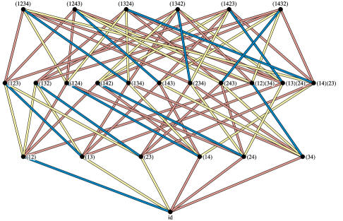
Figure 1. $\mathfrak{S}({4})$ with the Biane–Stanley edge-labeling (figure by M. LaCroix).

Since $\vec{W}^{r}({\pi_{1}},{\pi_{2}})=\vec{W}^{r}(\operatorname{id},{\pi_{1}}^{-1}{\pi_{2}})$, and since every permutation is either even or odd, the number $\vec{W}^{r}({\pi_{1}},{\pi_{2}})$ is nonzero if and only if $r=|{\pi_{1}}^{-1}{\pi_{2}}|+2g$ for some $g\in{\mathbb{N}}$. We may thus rewrite (30) as

(31) $$\operatorname{Wg}_{N}({\pi_{1}},{\pi_{2}})=\frac{(-1)^{|{\pi_{1}}^{-1}{\pi_{2}}|}}{N^{d+|{\pi_{1}}^{-1}{\pi_{2}}|}}\sum_{g=0}^{\infty}\frac{\vec{W}_{g}({\pi_{1}},{\pi_{2}})}{N^{2g}},$$

where $\vec{W}_{g}({\pi_{1}},{\pi_{2}})\mathrel{\mathop{\mathchar 58\relax}}=\vec{W}^{|{\pi_{1}}^{-1}{\pi_{2}}|+2g}({\pi_{1}},{\pi_{2}})$. The formulas (16) and (31) may be effectively combined to yield a sort of Feynman calculus for unitary matrix integrals, in which the role of Feynman diagrams is played by monotone walks on symmetric groups, see e.g. [GGPN16b, GGPN16a].

4.2. Quantum asymptotics

We now show that the quantum part of $\tau_{N}$ can be controlled even for $\hbar_{N}=\hbar$ fixed. In order to do this, we introduce a new permutation statistic defined by

$$\operatorname{defect}(\pi)\mathrel{\mathop{\mathchar 58\relax}}=\operatorname{aex}(\pi)-\operatorname{cyc}(\pi),\quad\pi\in\mathfrak{S}({d}).$$

Moreover, for any $k\in{\mathbb{N}}^{*}$ and ${\pi_{1}},\dots,\pi_{k}\in\mathfrak{S}({d})$, the quantity

$$\operatorname{genus}({\pi_{1}},\dots,\pi_{k})\mathrel{\mathop{\mathchar 58\relax}}=\frac{|{\pi_{1}}|+\dots+|\pi_{k}|-|{\pi_{1}}\dots\pi_{k}|}{2}$$

is a nonnegative integer; we refer to it as the genus of the $k$-tuple $({\pi_{1}},\dots,\pi_{k})$.

The following combinatorial result is a minor extension of the original results of Biane [Bia98, page 173], see Appendix C for a detailed proof and discussion of the relation to Biane’s work.

Lemma 4.1.

For any $\pi\in\mathfrak{S}({d})$, we have

$$\operatorname{defect}(\pi)\geq 0.$$

Moreover, for any permutations ${\pi_{1}},{\pi_{2}}\in\mathfrak{S}({d})$, we have

(32) $$\operatorname{defect}({\pi_{1}})+\operatorname{defect}({\pi_{2}}^{-1}\gamma)\leq 2\operatorname{genus}({\pi_{1}},{\pi_{1}}^{-1}{\pi_{2}},{\pi_{2}}^{-1}\gamma).$$

Theorem 4.2.

If $\hbar_{N}=O(1)$ as $N\to\infty$, then $\operatorname{Quantum}_{N}=O(1)$ as $N\rightarrow\infty$.

Proof.

By Theorem 2.7, the quantum part of $\tau_{N}$ may be written as

(33) $$\operatorname{Quantum}_{N}=\sum_{({\pi_{1}},{\pi_{2}})\in\mathfrak{S}({d})^{2}}N^{\operatorname{cyc}({\pi_{1}})+\operatorname{cyc}({\pi_{2}}^{-1}\gamma)-1}\operatorname{Wg}_{N}({\pi_{1}},{\pi_{2}})\ \mathbf{R}_{({\pi_{1}},{\pi_{2}})}(N),$$

where

$$\mathbf{R}_{({\pi_{1}},{\pi_{2}})}(N)= N^{\operatorname{defect}({\pi_{2}}^{-1}\gamma)}\ \overline{\mathbf{P}}_{{\pi_{1}}}^{\mathbf{A}}(N)\ \overline{\mathbf{Q}}_{{\pi_{2}}^{-1}\gamma}^{\mathbf{B}}(N)$$

$$+N^{\operatorname{defect}({\pi_{1}})}\ \overline{\mathbf{Q}}_{{\pi_{1}}}^{\mathbf{A}}(N)\ \overline{\mathbf{P}}_{{\pi_{2}}^{-1}\gamma}^{\mathbf{B}}(N)$$

$$+\hbar_{N}N^{\operatorname{defect}({\pi_{1}})+\operatorname{defect}({\pi_{2}}^{-1}\gamma)}\ \overline{\mathbf{Q}}_{{\pi_{1}}}^{\mathbf{A}}(N)\ \overline{\mathbf{Q}}_{{\pi_{2}}^{-1}\gamma}^{\mathbf{B}}(N).$$

We will show that each term in the sum (33) is $O(1)$.

By the first part of Lemma 4.1, nonnegativity of the defect statistic, as well as by Proposition 2.6 which shows that $\overline{\mathbf{P}}_{{\pi_{1}}}^{\mathbf{A}}(N)=O(1)$, $\overline{\mathbf{Q}}_{{\pi_{1}}}^{\mathbf{A}}(N)=O(1)$ and its counterpart for the matrix $B$ we have

$$\mathbf{R}_{({\pi_{1}},{\pi_{2}})}(N)=O\left(N^{\operatorname{defect}({\pi_{1}})+\operatorname{defect}({\pi_{2}}^{-1}\gamma)}\right)$$

for each $({\pi_{1}},{\pi_{2}})\in\mathfrak{S}({d})^{2}$.

Now, let us consider the order of the factor

$$N^{\operatorname{cyc}({\pi_{1}})+\operatorname{cyc}({\pi_{2}}^{-1}\gamma)-1}\operatorname{Wg}_{N}({\pi_{1}},{\pi_{2}}).$$

Invoking the expansion (31), for any $N\geq d$ we have

$$N^{\operatorname{cyc}({\pi_{1}})+\operatorname{cyc}({\pi_{2}}^{-1}\gamma)-1}\operatorname{Wg}_{N}({\pi_{1}},{\pi_{2}})\\ \begin{aligned} &=N^{\operatorname{cyc}({\pi_{1}})+\operatorname{cyc}({\pi_{2}}^{-1}\gamma)-1}\frac{(-1)^{|{\pi_{1}}^{-1}{\pi_{2}}|}}{N^{d+|{\pi_{1}}^{-1}{\pi_{2}}|}}\sum_{g=0}^{\infty}\frac{\vec{W}_{g}({\pi_{1}},{\pi_{2}})}{N^{2g}}\\ &=N^{-|{\pi_{1}}|-|{\pi_{1}}^{-1}{\pi_{2}}|-|{\pi_{2}}^{-1}\gamma|+|\gamma|}(-1)^{|{\pi_{1}}^{-1}{\pi_{2}}}\sum_{g=0}^{\infty}\frac{\vec{W}_{g}({\pi_{1}},{\pi_{2}})}{N^{2g}}\\ &=O(N^{-2\operatorname{genus}({\pi_{1}},{\pi_{1}}^{-1}{\pi_{2}},{\pi_{2}}^{-1}\gamma)}).\end{aligned}$$

We conclude that each term of $\operatorname{Quantum}_{N}$ is of order

$$N^{\operatorname{cyc}({\pi_{1}})+\operatorname{cyc}({\pi_{2}}^{-1}\gamma)-1}\operatorname{Wg}_{N}({\pi_{1}},{\pi_{2}})\mathbf{R}_{({\pi_{1}},{\pi_{2}})}(N)=\\ O\left(N^{\operatorname{defect}({\pi_{1}})+\operatorname{defect}({\pi_{2}}^{-1}\gamma)-2\operatorname{genus}({\pi_{1}},{\pi_{1}}^{-1}{\pi_{2}},{\pi_{2}}^{-1}\gamma)}\right),$$

and hence is $O(1)$ by the second part of Lemma 4.1. ∎

4.3. Classical asymptotics

We now deal with the asymptotics of the classical part of $\tau_{N}$.

Theorem 4.3.

Under the hypotheses of Theorem 1.3, the classical part of $\tau_{N}$ admits, for each $N\geq d$, the absolutely convergent series expansion

$$\operatorname{Classical}_{N}=\sum_{k=0}^{\infty}\frac{e_{k}(N)}{N^{2k}},$$

where

$$e_{k}(N)=\sum_{\begin{subarray}{c}(g,h)\in{\mathbb{N}}^{2}\\ g+h=k\end{subarray}}\sum_{\begin{subarray}{c}({\pi_{1}},{\pi_{2}})\in\mathfrak{S}({d})^{2}\\ \operatorname{genus}({\pi_{1}},{\pi_{1}}^{-1}{\pi_{2}},{\pi_{2}}^{-1}\gamma)=h\end{subarray}}(-1)^{|{\pi_{1}}^{-1}{\pi_{2}}|}\ \times\\ \times\vec{W}_{g}({\pi_{1}},{\pi_{2}})\ \overline{\mathbf{P}}_{{\pi_{1}}}^{\mathbf{A}}(N)\ \overline{\mathbf{P}}_{{\pi_{2}}^{-1}\gamma}^{\mathbf{B}}(N).$$

Proof.

According to Theorem 2.7 and the expansion (31), we have

$$\operatorname{Classical}_{N}=\\ \begin{aligned} \hskip 21.52771pt&=\sum_{({\pi_{1}},{\pi_{2}})\in\mathfrak{S}({d})^{2}}N^{\operatorname{cyc}({\pi_{1}})+\operatorname{cyc}({\pi_{2}}^{-1}\gamma)-1}\operatorname{Wg}_{N}({\pi_{1}},{\pi_{2}})\ \overline{\mathbf{P}}_{{\pi_{1}}}^{\mathbf{A}}(N)\ \overline{\mathbf{P}}_{{\pi_{2}}^{-1}\gamma}^{\mathbf{B}}(N)\\ &=\sum_{({\pi_{1}},{\pi_{2}})\in\mathfrak{S}({d})^{2}}N^{-2\operatorname{genus}({\pi_{1}},{\pi_{1}}^{-1}{\pi_{2}},{\pi_{2}}^{-1}\gamma)}(-1)^{|{\pi_{1}}^{-1}{\pi_{2}}|}\times\\ &\hskip 86.11084pt\times\overline{\mathbf{P}}_{{\pi_{1}}}^{\mathbf{A}}(N)\ \overline{\mathbf{P}}_{{\pi_{2}}^{-1}\gamma}^{\mathbf{B}}(N)\sum_{g=0}^{\infty}\frac{\vec{W}_{g}({\pi_{1}},{\pi_{2}})}{N^{2g}}\\ &=\sum_{g,h=0}^{\infty}\frac{1}{N^{2(g+h)}}\sum_{\begin{subarray}{c}({\pi_{1}},{\pi_{2}})\in\mathfrak{S}({d})^{2}\\ \operatorname{genus}({\pi_{1}},{\pi_{1}}^{-1}{\pi_{2}},{\pi_{2}}^{-1}\gamma)=h\end{subarray}}(-1)^{|{\pi_{1}}^{-1}{\pi_{2}}|}\times\\ &\hskip 86.11084pt\times\vec{W}_{g}({\pi_{1}},{\pi_{2}})\ \overline{\mathbf{P}}_{{\pi_{1}}}^{\mathbf{A}}(N)\ \overline{\mathbf{P}}_{{\pi_{2}}^{-1}\gamma}^{\mathbf{B}}(N)\\ &=\sum_{k=0}^{\infty}\sum_{\begin{subarray}{c}g,h\geq 0\\ g+h=k\end{subarray}}\frac{1}{N^{k}}\sum_{\begin{subarray}{c}({\pi_{1}},{\pi_{2}})\in\mathfrak{S}({d})^{2}\\ \operatorname{genus}({\pi_{1}},{\pi_{1}}^{-1}{\pi_{2}},{\pi_{2}}^{-1}\gamma)=h\end{subarray}}(-1)^{|{\pi_{1}}^{-1}{\pi_{2}}|}\times\\ &\hskip 86.11084pt\times\vec{W}_{g}({\pi_{1}},{\pi_{2}})\ \overline{\mathbf{P}}_{{\pi_{1}}}^{\mathbf{A}}(N)\ \overline{\mathbf{P}}_{{\pi_{2}}^{-1}\gamma}^{\mathbf{B}}(N).\end{aligned}$$

∎

4.4. Semiclassical asymptotics and freeness

Combining Theorems 4.3 and 4.2, we obtain the following corollary.

Corollary 4.4.

For any sequence $\hbar_{N}=O(1)$, we have

$$\tau_{N}=\operatorname{Classical}_{N}+O(\hbar_{N})$$

as $N\rightarrow\infty$. In particular, if $\hbar_{N}=o(N^{-2l})$ as $N\rightarrow\infty$, then

$$\tau_{N}=\operatorname{Classical}_{N}+o(N^{-2l})=\sum_{k=0}^{l}\frac{e_{k}(N)}{N^{2k}}+o(N^{-2l}).$$

Let us now explain how the the $l=0$ case of Corollary 4.4 yields the proof of Theorem 1.3. Assuming only $\hbar_{N}=o(1)$ as $N\to\infty$, Corollary 4.4 implies

$$\tau_{N}=\operatorname{Classical}_{N}+o(1)=e_{0}(N)+o(1)$$

as $N\rightarrow\infty$, with

$$e_{0}(N)=\sum_{\begin{subarray}{c}({\pi_{1}},{\pi_{2}})\in\mathfrak{S}({d})^{2}\\ \operatorname{genus}({\pi_{1}},{\pi_{1}}^{-1}{\pi_{2}},{\pi_{2}}^{-1}\gamma)=0\end{subarray}}(-1)^{|{\pi_{1}}^{-1}{\pi_{2}}|}\ \vec{W}_{0}({\pi_{1}},{\pi_{2}})\ \overline{\mathbf{P}}_{{\pi_{1}}}^{\mathbf{A}}(N)\ \overline{\mathbf{P}}_{{\pi_{2}}^{-1}\gamma}^{\mathbf{B}}(N).$$

Now, under the hypotheses of Theorem 1.3, the limits

$$\overline{\mathbf{P}}_{{\pi_{1}}}^{\mathbf{A}}=\lim_{N\to\infty}\overline{\mathbf{P}}_{{\pi_{1}}}^{\mathbf{A}}(N)\quad\text{ and }\quad\overline{\mathbf{P}}_{{\pi_{2}}^{-1}\gamma}^{\mathbf{B}}=\lim_{N\to\infty}\overline{\mathbf{P}}_{{\pi_{2}}^{-1}\gamma}^{\mathbf{B}}(N)$$

exists, and are polynomials in $x_{1},\dots,x_{|p|}$ and $y_{1},\dots,y_{|q|}$ given explicitly by the universal form (23) of the classical component. We thus have

$$\lim_{N\to\infty}\tau_{N}=\sum_{\begin{subarray}{c}({\pi_{1}},{\pi_{2}})\in\mathfrak{S}({d})^{2}\\ \operatorname{genus}({\pi_{1}},{\pi_{1}}^{-1}{\pi_{2}},{\pi_{2}}^{-1}\gamma)=0\end{subarray}}(-1)^{|{\pi_{1}}^{-1}{\pi_{2}}|}\ \vec{W}_{0}({\pi_{1}},{\pi_{2}})\ \overline{\mathbf{P}}_{{\pi_{1}}}^{\mathbf{A}}\ \overline{\mathbf{P}}_{{\pi_{2}}^{-1}\gamma}^{\mathbf{B}}.$$

This is exactly asymptotic freeness, see Appendix A. Hence, Theorem 1.3 is proved.

5. Covariance of BPP Observables

In this section we explain how the mean value analysis carried out in Sections 2 and 4, which yields the semiclassical/large-dimension asymptotics of the $1$-point functions of BPP observables of the LR process, can be extended to higher correlation functions. We limit our discussion to the connected $2$-point functions (covariances)

$$\langle\overline{\wp}_{k_{1}}^{(N)}\overline{\wp}_{k_{2}}^{(N)}\rangle_{c}=\langle\overline{\wp}_{k_{1}}^{(N)}\overline{\wp}_{k_{2}}^{(N)}\rangle-\langle\overline{\wp}_{k_{1}}^{(N)}\rangle\langle\overline{\wp}_{k_{2}}^{(N)}\rangle,$$

since these are what we need to understand in order to obtain Theorem 1.4, the Law of Large Numbers for BPP observables of the LR process.

5.1. Covariance setup

According to Biane’s formula (12), the covariance of the classical random variables $\overline{\wp}_{k_{1}}^{(N)},\overline{\wp}_{k_{2}}^{(N)}$ coincides with the covariance of the quantum random variables $\operatorname{tr}(C_{N}^{k_{1}}),\operatorname{tr}(C_{N}^{k_{2}})$:

$$\langle\overline{\wp}_{k_{1}}^{(N)}\overline{\wp}_{k_{2}}^{(N)}\rangle_{c}={\mathbb{E}}[\operatorname{tr}(C_{N}^{k_{1}})\operatorname{tr}(C_{N}^{k_{2}})]-{\mathbb{E}}[\operatorname{tr}(C_{N}^{k_{1}})]\ {\mathbb{E}}\operatorname{tr}[(C_{N}^{k_{2}})]$$

for any $k_{1},k_{2}\in{\mathbb{N}}^{*}$, where $C_{N}=A_{N}+B_{N}$. For example, in the case of the simplest connected $2$-point function, the variance of $\overline{\wp}_{1}^{(N)}$, we have

$$\langle\overline{\wp}_{1}^{(N)}\overline{\wp}_{1}^{(N)}\rangle_{c} ={\mathbb{E}}[\operatorname{tr}(C_{N})\operatorname{tr}(C_{N})]-{\mathbb{E}}[\operatorname{tr}(C_{N})]{\mathbb{E}}[\operatorname{tr}(C_{N})]$$

$$={\mathbb{E}}[\operatorname{tr}(A_{N})\operatorname{tr}(A_{N})]-{\mathbb{E}}[\operatorname{tr}(A_{N})]\ {\mathbb{E}}[\operatorname{tr}(A_{N})]$$

$$+{\mathbb{E}}[\operatorname{tr}(A_{N})\operatorname{tr}(B_{N})]-{\mathbb{E}}[\operatorname{tr}(A_{N})]\ {\mathbb{E}}[\operatorname{tr}(B_{N})]$$

$$+{\mathbb{E}}[\operatorname{tr}(B_{N})\operatorname{tr}(A_{N})]-{\mathbb{E}}[\operatorname{tr}(B_{N})]\ {\mathbb{E}}[\operatorname{tr}(A_{N})]$$

$$+{\mathbb{E}}[\operatorname{tr}(B_{N})\operatorname{tr}(B_{N})]-{\mathbb{E}}[\operatorname{tr}(B_{N})]\ {\mathbb{E}}[\operatorname{tr}(B_{N})].$$

In general, in order to compute $\langle\overline{\wp}_{k_{1}}^{(N)}\overline{\wp}_{k_{2}}^{(N)}\rangle_{c}$ in the semiclassical/large-dimension limit, we need to be able to estimate differences of the form

$${\mathbb{E}}\left[\operatorname{tr}(A_{N}^{p_{1}(1)}B_{N}^{q_{1}(1)}\cdots A_{N}^{p_{1}(d_{1})}B_{N}^{q_{1}(d_{1})})\operatorname{tr}(A_{N}^{p_{2}(1)}B_{N}^{q_{2}(1)}\cdots A_{N}^{p_{2}(d_{2})}B_{N}^{q_{2}(d_{2})})\right]$$

$$- {\mathbb{E}}\left[\operatorname{tr}(A_{N}^{p_{1}(1)}B_{N}^{q_{1}(1)}\cdots A_{N}^{p_{1}(d_{1})}B_{N}^{q_{1}(d_{1})})\right]\ {\mathbb{E}}\left[\operatorname{tr}(A_{N}^{p_{2}(1)}B_{N}^{q_{2}(1)}\cdots A_{N}^{p_{2}(d_{2})}B_{N}^{q_{2}(d_{2})})\right]$$

in the semiclassical/large-dimension limit, where $d_{1},d_{2}\in{\mathbb{N}}^{*}$ are fixed positive integers and $p_{1},q_{1}\colon[d_{1}]\to{\mathbb{N}}$ and $p_{2},q_{d}\colon[d_{2}]\to{\mathbb{N}}$ are fixed functions. Let us write

$$\tau_{12}^{(N)}\mathrel{\mathop{\mathchar 58\relax}}={\mathbb{E}}\left[\operatorname{tr}(A_{N}^{p_{1}(1)}B_{N}^{q_{1}(1)}\cdots A_{N}^{p_{1}(d_{1})}B_{N}^{q_{1}(d_{1})})\operatorname{tr}(A_{N}^{p_{2}(1)}B_{N}^{q_{2}(1)}\cdots A_{N}^{p_{2}(d_{2})}B_{N}^{q_{2}(d_{2})})\right]$$

and

$$\tau_{1}^{(N)} \mathrel{\mathop{\mathchar 58\relax}}={\mathbb{E}}\operatorname{tr}(A_{N}^{p_{1}(1)}B_{N}^{q_{1}(1)}\cdots A_{N}^{p_{1}(d_{1})}B_{N}^{q_{1}(d_{1})})$$

$$\tau_{2}^{(N)} \mathrel{\mathop{\mathchar 58\relax}}={\mathbb{E}}\operatorname{tr}(A_{N}^{p_{2}(1)}B_{N}^{q_{2}(1)}\cdots A_{N}^{p_{2}(d_{2})}B_{N}^{q_{2}(d_{2})})$$

for these quantities, so that our goal is to estimate the difference

$$\tau_{12}^{(N)}-\tau_{1}^{(N)}\tau_{2}^{(N)}$$

in the semiclassical/large-dimension limit. In view of our analysis of mean values in Sections 2 and 4, the second term is understood. It remains to analyze the first term, $\tau_{12}^{(N)}$, and in order to do this we will generalize the approach developed above.

5.2. $2$-point functions at the Planck scale

Let us rewrite $\tau_{12}^{(N)}$ as follows. Put $d=d_{1}+d_{2}$, and define functions $p,q\colon[d]\to{\mathbb{N}}$ by

$$p|_{[d_{1}]} =p_{1}, p|_{[d_{1}+1,d]} =p_{2}$$

$$q|_{[d_{1}]} =q_{1}, q|_{[d_{1}+1,d]} =q_{2}.$$

We then have

$$\tau_{12}^{(N)}={\mathbb{E}}\left[\operatorname{tr}(A_{N}^{p(1)}B_{N}^{q(1)}\cdots A_{N}^{p(d_{1})}B_{N}^{q(d_{1})})\right.\\ \left.\operatorname{tr}(A_{N}^{p(d_{1}+1)}B_{N}^{q(d_{1}+1)}\cdots A_{N}^{p(d_{1}+d_{2})}B_{N}^{q(d_{1}+d_{2})})\right].$$

It will be convenient to affect the same notational change for the quantities $\tau_{1}^{(N)}$ and $\tau_{2}^{(N)}$, that is we write

$$\tau_{1}^{(N)} ={\mathbb{E}}\operatorname{tr}(A_{N}^{p(1)}B_{N}^{q(1)}\cdots A_{N}^{p(d_{1})}B_{N}^{q(d_{1})}),$$

$$\tau_{2}^{(N)} ={\mathbb{E}}\operatorname{tr}(A_{N}^{p(d_{1}+1)}B_{N}^{q(d_{1}+1)}\cdots A_{N}^{p(d_{1}+d_{2})}B_{N}^{q(d_{1}+d_{2})}).$$

We now analyze $\tau_{12}^{(N)}$ following the same steps as in Sections 2 and 4.

5.2.1. Unitary invariance

Proposition 5.1.

Define a function $f\colon\mathrm{U}(N)\rightarrow{\mathbb{C}}$ by

$$f_{N}(U)\mathrel{\mathop{\mathchar 58\relax}}={\mathbb{E}}\left[\operatorname{tr}\left(UA_{N}^{p(1)}U^{-1}B_{N}^{q(1)}\cdots UA_{N}^{p(d_{1})}U^{-1}B_{N}^{q(d_{1})}\right)\right.\times\\ \times\left.\operatorname{tr}\left(UA_{N}^{p(d_{1}+1)}U^{-1}B_{N}^{q(d_{1}+1)}\cdots UA_{N}^{p(d_{1}+d_{2})}U^{-1}B_{N}^{q(d_{1}+d_{2})}\right)\right].$$

Then, $f_{N}$ is constant, being equal to $\tau_{12}^{(N)}$ for all $U\in\mathrm{U}(N)$.

As a consequence of this invariance, we have

$$\tau_{12}^{(N)}=\int_{\mathrm{U}(N)}f_{N}(U)\mathrm{d}U.$$

We want to use this in exactly the same way as we did in our mean value computation.

Expanding the first trace yields the sum

$$\frac{1}{N}\sum_{r_{1}\colon[4d_{1}]\to[N]}U_{r_{1}(1)r_{1}(2)}\left(A_{N}^{p(1)}\right)_{r_{1}(2)r_{1}(3)}U^{-1}_{r_{1}(3)r_{1}(4)}\left(B_{N}^{q(1)}\right)_{r_{1}(4)r_{1}(5)}\cdots\\ \cdots U_{r_{1}(4d_{1}-3)r_{1}(4d_{1}-2)}\left(A_{N}^{p(d_{1})}\right)_{r_{1}(4d_{1}-2)r_{1}(4d_{1}-1)}U^{-1}_{r_{1}(4d_{1}-1)r_{1}(4d_{1})}\left(B_{N}^{q(d_{1})}\right)_{r_{1}(4d_{1})r_{1}(1)}.$$

Expanding the second trace yields the sum

$$\frac{1}{N}\sum_{r_{2}\colon[4d_{2}]\to[N]}U_{r_{2}(1)r_{2}(2)}\left(A_{N}^{p(d_{1}+1)}\right)_{r_{2}(2)r_{2}(3)}U^{-1}_{r_{2}(3)r_{2}(4)}\left(B_{N}^{q(d_{1}+1)}\right)_{r_{2}(4)r_{2}(5)}\cdots\\ \cdots U_{r_{2}(4d_{2}-3)r_{2}(4d_{2}-2)}\left(A_{N}^{p(d_{1}+d_{2})}\right)_{r_{2}(4d_{2}-2)r_{2}(4d_{2}-1)}U^{-1}_{r_{2}(4d_{2}-1)r_{2}(4d_{2})}\left(B_{N}^{q(d_{1}+d_{2})}\right)_{r_{2}(4d_{2})r_{2}(1)}.$$

For the first trace, let us reparametrize the summation index $r_{1}\colon[4d_{1}]\to[N]$ by a quadruple of functions $i_{1},j_{1},i_{1}^{\prime},j_{1}^{\prime}\colon[d_{1}]\to[N]$ according to

$$\big{(}r_{1}(1),r_{1}(2),r_{1}(3),r_{1}(4),\dots,r_{1}(4d_{1}-3),r_{1}(4d_{1}-2),r_{1}(4d_{1}-1),r_{1}(4d_{1})\big{)}\\ =\big{(}i_{1}(1),j_{1}(1),j_{1}^{\prime}(1),i_{1}^{\prime}(1),\dots,i_{1}(d_{1}),j_{1}(d_{1}),j_{1}^{\prime}(d_{1}),i_{1}^{\prime}(d_{1})\big{)}.$$

Then, the above expansion of the first trace becomes

$$\frac{1}{N}\sum_{i_{1},j_{1},_{1}i^{\prime},j_{1}^{\prime}\colon[d_{1}]\to[N]}L_{N}(i_{1},j_{1},i_{1}^{\prime},j_{1}^{\prime})\ \prod_{k=1}^{d_{1}}\left(A_{N}^{p(k)}\right)_{j_{1}(k)j_{1}^{\prime}(k)}\left(B_{N}^{q(k)}\right)_{i_{1}^{\prime}(k)i_{1}\gamma_{1}(k)}$$

$$= \frac{1}{N}\sum_{i_{1},j_{1},i_{1}^{\prime},j_{1}^{\prime}\colon[d_{1}]\to[N]}L_{N}(i_{1},j_{1},i_{1}^{\prime},j_{1}^{\prime})\ \prod_{k=1}^{d_{1}}\left(A_{N}^{p(k)}\right)_{j_{1}(k)j_{1}^{\prime}(k)}\prod_{k=1}^{d_{1}}\left(B_{N}^{q(k)}\right)_{i_{1}^{\prime}(k)i_{1}\gamma_{1}(k)},$$

where

$$L_{N}(i_{1},j_{1},i_{1}^{\prime},j_{1}^{\prime})=\prod_{k=1}^{d_{1}}U_{i_{1}(k)j_{1}(k)}\overline{U}_{i_{1}^{\prime}(k)j_{1}^{\prime}(k)},$$

and $\gamma_{1}$ is the cycle $(1\ 2\ \dots\ d_{1})$ in $\mathfrak{S}({d_{1}+d_{2}})$.

Similarly, if we reparametrize the summation index $r_{2}\colon[4d_{2}]\to[N]$ by a quadruple of functions $i_{2},j_{2},i_{2}^{\prime},j_{2}^{\prime}\colon[d_{2}]\to[N]$ according to

$$\big{(}r_{2}(1),r_{2}(2),r_{2}(3),r_{2}(4),\dots,r_{2}(4d_{2}-3),r_{2}(4d_{2}-2),r_{2}(4d_{2}-1),r_{2}(4d_{2})\big{)}\\ =\big{(}i_{2}(d_{1}+1),j_{2}(d_{1}+1),j_{2}^{\prime}(d_{1}+1),i_{2}^{\prime}(d_{1}+1),\dots,i_{2}(d),j_{2}(d),j_{2}^{\prime}(d),i_{2}^{\prime}(d)\big{)},$$

the expansion of the second trace takes the form

$$\frac{1}{N}\sum_{i_{2},j_{2},i_{2}^{\prime},j_{2}^{\prime}\colon[d_{1}+1,d_{1}+d_{2}]\to[N]}L_{N}(i_{2},j_{2},i_{2}^{\prime},j_{2}^{\prime})\ \prod_{k=d_{1}+1}^{d_{1}+d_{2}}\left(A_{N}^{p(k)}\right)_{j_{2}(k)j_{2}^{\prime}(k)}\left(B_{N}^{q(k)}\right)_{i_{2}^{\prime}(k)i_{2}\gamma_{2}^{\prime}(k)}$$

$$= \frac{1}{N}\sum_{i_{2},j_{2},i_{2}^{\prime},j_{2}^{\prime}\colon[d_{1}+1,d_{1}+d_{2}]\to[N]}L_{N}(i_{2},j_{2},i_{2}^{\prime},j_{2}^{\prime})\ \prod_{k=d_{1}+1}^{d_{1}+d_{2}}\left(A_{N}^{p(k)}\right)_{j_{2}(k)j_{2}^{\prime}(k)}\prod_{k=1}^{d_{2}}\left(B_{N}^{q(k)}\right)_{i_{2}^{\prime}(k)i_{2}\gamma_{2}^{\prime}(k)},$$

where

$$L_{N}(i_{2},j_{2},i_{2}^{\prime},j_{2}^{\prime})=\prod_{k=d_{1}+1}^{d_{1}+d_{2}}U_{i_{2}(k)j_{2}(k)}\overline{U}_{i_{2}^{\prime}(k)j_{2}^{\prime}(k)},$$

and $\gamma_{2}^{\prime}$ is the cycle $(d_{1}+1\ d_{1}+2\ \dots\ d_{1}+d_{2})$ in $\mathfrak{S}({d_{1}+d_{2}})$.

We now smash the expansions of the two traces together to get the huge compound expansion

$$\frac{1}{N^{2}}\sum_{i_{1},j_{1},_{1}i^{\prime},j_{1}^{\prime}\colon[d_{1}]\to[N]}\ \sum_{i_{2},j_{2},i_{2}^{\prime},j_{2}^{\prime}\colon[d_{1}+1,d_{1}+d_{2}]\to[N]}L_{N}(i_{1},j_{1},i_{1}^{\prime},j_{1}^{\prime})\ L_{N}(i_{2},j_{2},i_{2}^{\prime},j_{2}^{\prime})$$

$$\times\prod_{k=1}^{d_{1}}\left(A_{N}^{p(k)}\right)_{j_{1}(k)j_{1}^{\prime}(k)}\prod_{k=d_{1}+1}^{d_{1}+d_{2}}\left(A_{N}^{p(k)}\right)_{j_{2}(k)j_{2}^{\prime}(k)}\prod_{k=1}^{d_{1}}\left(B_{N}^{q(k)}\right)_{i_{1}^{\prime}(k)i_{1}\gamma_{1}(k)}\prod_{k=d_{1}+1}^{d_{1}+d_{2}}\left(B_{N}^{q(k)}\right)_{i_{2}^{\prime}(k)i_{2}\gamma_{2}^{\prime}(k)}$$

$$= \frac{1}{N^{2}}\sum_{i,j,i^{\prime},j^{\prime}\colon[d_{1}+d_{2}]\to[N]}\ L_{N}(i,j,i^{\prime},j^{\prime})\prod_{k=1}^{d_{1}+d_{2}}\left(A_{N}^{p(k)}\right)_{j(k)j^{\prime}(k)}\prod_{k=1}^{d_{1}+d_{2}}\left(B_{N}^{q(k)}\right)_{i^{\prime}(k)i\gamma_{1}\gamma_{2}^{\prime}(k)},$$

where

$$L_{N}(i,j,i^{\prime},j^{\prime})=\prod_{k=1}^{d_{1}+d_{2}}U_{i(k)j(k)}\ \overline{U}_{i^{\prime}(k)j^{\prime}(k)}.$$

Thus, we obtain the following representation of $\tau_{12}^{(N)}$:

$$\tau_{12}^{(N)}=\frac{1}{N^{2}}\sum_{i,j,i^{\prime},j^{\prime}\colon[d_{1}+d_{2}]\to[N]}\ I_{N}(i,j,i^{\prime},j^{\prime})\times\\ \times{\mathbb{E}}\left[\prod_{k=1}^{d_{1}+d_{2}}\left(A_{N}^{p(k)}\right)_{j(k)j^{\prime}(k)}\right]{\mathbb{E}}\left[\prod_{k=1}^{d_{1}+d_{2}}\left(B_{N}^{q(k)}\right)_{i^{\prime}(k)i\gamma_{1}\gamma_{2}^{\prime}(k)}\right],$$

where

$$I_{N}(i,j,i^{\prime},j^{\prime})=\int_{\mathrm{U}(N)}L_{N}(i,j,i^{\prime},j^{\prime})\mathrm{d}U.$$

Plugging (16) into our calculation above eliminates the indices $i^{\prime},j^{\prime}$ and produces the formula

$$\tau_{12}^{(N)}=\frac{1}{N^{2}}\sum_{({\pi_{1}},{\pi_{2}})\in\mathfrak{S}({d_{1}+d_{2}})^{2}}\operatorname{Wg}_{N}({\pi_{1}},{\pi_{2}})\ {\mathbb{E}}[S^{A}_{{\pi_{1}}}]\ {\mathbb{E}}[S^{B}_{{\pi_{2}}^{-1}\gamma_{1}\gamma_{2}^{\prime}}],$$

where

$$S^{A}_{{\pi_{1}}}\mathrel{\mathop{\mathchar 58\relax}}= \sum_{i\colon[d_{1}+d_{2}]\to[N]}\prod_{k=1}^{d_{1}+d_{2}}\left(A_{N}^{p(k)}\right)_{i(k)i{\pi_{1}}(k)}$$

and

$$S^{B}_{{\pi_{2}}^{-1}\gamma_{1}\gamma_{2}^{\prime}}\mathrel{\mathop{\mathchar 58\relax}}= \sum_{i\colon[d_{1}+d_{2}]\to[N]}\prod_{k=1}^{d_{1}+d_{2}}\left(B_{N}^{q(k)}\right)_{i(k)i{\pi_{2}}^{-1}\gamma_{1}\gamma_{2}^{\prime}(k)}.$$

This generalizes (17) from the expected trace to the expected product of two traces; the formula could be generalized to the expected product of any finite number of traces in just the same way.

Our goal now is to express the operators $S^{A}_{{\pi_{1}}}$ and $S^{B}_{{\pi_{2}}^{-1}\gamma_{1}\gamma_{2}^{\prime}}$ in terms of the operators

$$\operatorname{tr}A_{N},\operatorname{tr}A_{N}^{2},\dots\quad\text{ and }\operatorname{tr}B_{N},\operatorname{tr}B_{N}^{2},\dots.$$

Just like in the mean value computation, we lift the problem to the universal enveloping algebra and use Biasimirs.

5.2.2. Biasimirs again

The operators $S^{A}_{\pi_{1}}$ and $S^{B}_{{\pi_{2}}^{-1}\gamma_{1}\gamma_{2}^{\prime}}$ are, up to tensoring with an identity operator, images of Biasimirs in irreducible representations:

$$S^{A}_{{\pi_{1}}} =\rho_{N}(C_{{\pi_{1}}}^{(p)})\otimes I_{\mathbf{W}_{N}}$$

$$S^{B}_{{\pi_{2}}^{-1}\gamma_{1}\gamma_{2}^{\prime}} =I_{\mathbf{V}_{N}}\otimes\sigma_{N}(C_{{\pi_{2}}^{-1}\gamma_{1}\gamma_{2}^{\prime}}^{(q)}).$$

Each of the Biasimirs $C_{\pi_{1}}^{(p)}$ and $C_{{\pi_{2}}^{-1}\gamma_{1}\gamma_{2}^{\prime}}^{(q)}$ has its own classical/quantum decomposition:

$$C_{\pi_{1}}^{(p)} =\mathbf{P}_{\pi_{1}}^{(p)}(C_{1},\dots,C_{|p|})+\hbar_{N}\mathbf{Q}_{\pi_{1}}^{(p)}(\hbar_{N},N,C_{1},\dots,C_{|p|})$$

$$C_{{\pi_{2}}^{-1}\gamma_{1}\gamma_{2}^{\prime}}^{(q)} =\mathbf{P}_{{\pi_{2}}^{-1}\gamma_{1}\gamma_{2}^{\prime}}^{(q)}(C_{1},\dots,C_{|q|})+\hbar_{N}\mathbf{Q}_{{\pi_{2}}^{-1}\gamma_{1}\gamma_{2}^{\prime}}^{(q)}(\hbar_{N},N,C_{1},\dots,C_{|q|}).$$

Now we come back to the operators $S^{A}_{\pi_{1}}$ and $S^{B}_{{\pi_{2}}^{-1}\gamma_{1}\gamma_{2}^{\prime}}$. First, we have that

$$S^{A}_{\pi_{1}}=\mathbf{P}_{\pi_{1}}^{(p)}(\operatorname{Tr}A_{N},\dots,\operatorname{Tr}A_{N}^{|p|})+\hbar_{N}\mathbf{Q}_{\pi_{1}}^{(p)}(\hbar_{N},N,\operatorname{Tr}A_{N},\dots,\operatorname{Tr}A_{N}^{|p|}).$$

Let us rewrite this in terms of normalized traces. Put

$$\overline{\mathbf{P}}_{{\pi_{1}}}^{\mathbf{A}} \mathrel{\mathop{\mathchar 58\relax}}=\frac{1}{N^{\operatorname{cyc}({\pi_{1}})}}\mathbf{P}_{\pi_{1}}^{(p)}\left(\operatorname{Tr}A_{N},\dots,\operatorname{Tr}A_{N}^{|p|}\right),$$

$$\overline{\mathbf{Q}}_{{\pi_{1}}}^{\mathbf{A}} \mathrel{\mathop{\mathchar 58\relax}}=\frac{1}{N^{\operatorname{aex}({\pi_{1}})}}\mathbf{Q}_{\pi_{1}}^{(p)}\left(\hbar_{N},N,\operatorname{Tr}A_{N},\dots,\operatorname{Tr}A_{N}^{|p|}\right).$$

$\overline{\mathbf{P}}_{{\pi_{1}}}^{\mathbf{A}}$ is an explicit polynomial in the operators

$$\operatorname{tr}A_{N},\operatorname{tr}A_{N}^{2},\dots,\operatorname{tr}A_{N}^{|p|},$$

while $\overline{\mathbf{Q}}_{{\pi_{1}}}^{\mathbf{A}}$ is a polynomial in the numbers $\hbar_{N},N^{-1}$ and the operators

$$\operatorname{tr}A_{N},\operatorname{tr}A_{N}^{2},\dots,\operatorname{tr}A_{N}^{|p|}.$$

We thus have

$$S^{A}_{\pi_{1}}=N^{\operatorname{cyc}({\pi_{1}})}\overline{\mathbf{P}}_{{\pi_{1}}}^{\mathbf{A}}+\hbar_{N}N^{\operatorname{aex}({\pi_{1}})}\overline{\mathbf{Q}}_{{\pi_{1}}}^{\mathbf{A}}.$$

Now we want to apply the expectation ${\mathbb{E}}$ to both sides of this identity in ${\mathcal{A}}_{N}$ to get an identity in ${\mathbb{C}}$. We set

$$\overline{\mathbf{P}}_{{\pi_{1}}}^{\mathbf{A}}(N) \mathrel{\mathop{\mathchar 58\relax}}={\mathbb{E}}\overline{\mathbf{P}}_{{\pi_{1}}}^{\mathbf{A}}=\frac{1}{N^{\operatorname{cyc}({\pi_{1}})}}\mathbf{P}_{\pi_{1}}^{(p)}\left({\mathbb{E}}\operatorname{Tr}A_{N},\dots,{\mathbb{E}}\operatorname{Tr}A_{N}^{|p|}\right),$$

$$\overline{\mathbf{Q}}_{{\pi_{1}}}^{\mathbf{A}}(N) \mathrel{\mathop{\mathchar 58\relax}}={\mathbb{E}}\overline{\mathbf{Q}}_{{\pi_{1}}}^{\mathbf{A}}=\frac{1}{N^{\operatorname{aex}({\pi_{1}})}}\mathbf{Q}_{\pi_{1}}^{(p)}\left(\hbar_{N},N,{\mathbb{E}}\operatorname{Tr}A_{N},\dots,{\mathbb{E}}\operatorname{Tr}A_{N}^{|p|}\right);$$

the first of these is a polynomial in the numbers

$${\mathbb{E}}\operatorname{tr}A_{N},{\mathbb{E}}\operatorname{tr}A_{N}^{2},\dots,{\mathbb{E}}\operatorname{tr}A_{N}^{|p|},$$

while the second is a polynomial in the numbers

$$\hbar_{N},N^{-1},{\mathbb{E}}\operatorname{tr}A_{N},{\mathbb{E}}\operatorname{tr}A_{N}^{2},\dots,{\mathbb{E}}\operatorname{tr}A_{N}^{|p|}.$$

We conclude that

$${\mathbb{E}}[S^{A}_{\pi_{1}}]=N^{\operatorname{cyc}({\pi_{1}})}\overline{\mathbf{P}}_{{\pi_{1}}}^{\mathbf{A}}(N)+\hbar_{N}N^{\operatorname{aex}({\pi_{1}})}\overline{\mathbf{Q}}_{{\pi_{1}}}^{\mathbf{A}}(N).$$

Second, we have that

$$S^{B}_{{\pi_{2}}^{-1}\gamma_{1}\gamma_{2}^{\prime}}=\mathbf{P}_{{\pi_{2}}^{-1}\gamma_{1}\gamma_{2}^{\prime}}^{(q)}(\operatorname{Tr}B_{N},\dots,\operatorname{Tr}B_{N}^{|q|})+\\ +\hbar_{N}\mathbf{Q}^{(q)}_{{\pi_{2}}^{-1}\gamma_{1}\gamma_{2}^{\prime}}(\hbar_{N},N,\operatorname{Tr}B_{N},\dots,\operatorname{Tr}B_{N}^{|q|}).$$

Once again, let us rewrite this in terms of normalized traces. Put

$$\overline{\mathbf{P}}_{{\pi_{2}}^{-1}\gamma_{1}\gamma_{2}^{\prime}}^{\mathbf{B}} \mathrel{\mathop{\mathchar 58\relax}}=\frac{1}{N^{\operatorname{cyc}({\pi_{2}}^{-1}\gamma_{1}\gamma_{2}^{\prime})}}\mathbf{P}_{{\pi_{2}}^{-1}\gamma_{1}\gamma_{2}^{\prime}}^{(q)}\left(\operatorname{Tr}B_{N},\dots,\operatorname{Tr}B_{N}^{|q|}\right),$$

$$\overline{\mathbf{Q}}_{{\pi_{2}}^{-1}\gamma_{1}\gamma_{2}^{\prime}}^{\mathbf{B}} \mathrel{\mathop{\mathchar 58\relax}}=\frac{1}{N^{\operatorname{aex}({\pi_{2}}^{-1}\gamma_{1}\gamma_{2}^{\prime})}}\mathbf{Q}_{{\pi_{2}}^{-1}\gamma_{1}\gamma_{2}^{\prime}}^{(q)}\left(\hbar_{N},N,\operatorname{Tr}B_{N},\dots,\operatorname{Tr}B_{N}^{|q|}\right).$$

$\overline{\mathbf{P}}_{{\pi_{2}}^{-1}\gamma_{1}\gamma_{2}^{\prime}}^{\mathbf{B}}$ is an explicit polynomial in the operators

$$\operatorname{tr}B_{N},\operatorname{tr}B_{N}^{2},\dots,\operatorname{tr}B_{N}^{|q|},$$

while $\overline{\mathbf{Q}}_{{\pi_{2}}^{-1}\gamma_{1}\gamma_{2}^{\prime}}^{\mathbf{B}}$ is a polynomial in the numbers $\hbar_{N},N^{-1}$ and the operators

$$\operatorname{tr}B_{N},\operatorname{tr}B_{N}^{2},\dots,\operatorname{tr}B_{N}^{|q|}.$$

We thus have

$$S^{B}_{{\pi_{2}}^{-1}\gamma_{1}\gamma_{2}^{\prime}}=N^{\operatorname{cyc}({\pi_{2}}^{-1}\gamma_{1}\gamma_{2}^{\prime})}\overline{\mathbf{P}}_{{\pi_{2}}^{-1}\gamma_{1}\gamma_{2}^{\prime}}^{\mathbf{B}}+\hbar_{N}N^{\operatorname{aex}({\pi_{2}}^{-1}\gamma_{1}\gamma_{2}^{\prime})}\overline{\mathbf{Q}}_{{\pi_{2}}^{-1}\gamma_{1}\gamma_{2}^{\prime}}^{\mathbf{B}}.$$

We apply ${\mathbb{E}}$ to both sides of this identity in ${\mathcal{A}}_{N}$ to get an identity in ${\mathbb{C}}$. As above, we declare

$$\overline{\mathbf{P}}_{{\pi_{2}}^{-1}\gamma_{1}\gamma_{2}^{\prime}}^{\mathbf{B}}(N) \mathrel{\mathop{\mathchar 58\relax}}={\mathbb{E}}\overline{\mathbf{P}}_{{\pi_{2}}^{-1}\gamma_{1}\gamma_{2}^{\prime}}^{\mathbf{B}}=$$

$$\hskip 21.52771pt\frac{1}{N^{\operatorname{cyc}({\pi_{2}}^{-1}\gamma_{1}\gamma_{2}^{\prime})}}\mathbf{P}_{{\pi_{2}}^{-1}\gamma_{1}\gamma_{2}^{\prime}}^{(q)}\left({\mathbb{E}}\operatorname{Tr}B_{N},\dots,{\mathbb{E}}\operatorname{Tr}B_{N}^{|q|}\right),$$

$$\overline{\mathbf{Q}}_{{\pi_{2}}^{-1}\gamma_{1}\gamma_{2}^{\prime}}^{\mathbf{B}}(N) \mathrel{\mathop{\mathchar 58\relax}}={\mathbb{E}}\overline{\mathbf{Q}}_{{\pi_{2}}^{-1}\gamma_{1}\gamma_{2}^{\prime}}^{\mathbf{B}}=$$

$$\frac{1}{N^{\operatorname{aex}({\pi_{2}}^{-1}\gamma_{1}\gamma_{2}^{\prime})}}\mathbf{Q}_{{\pi_{2}}^{-1}\gamma_{1}\gamma_{2}^{\prime}}^{(q)}\left(\hbar_{N},N,{\mathbb{E}}\operatorname{Tr}B_{N},\dots,{\mathbb{E}}\operatorname{Tr}B_{N}^{|q|}\right).$$

The first of these is a polynomial in the numbers

$${\mathbb{E}}\operatorname{tr}B_{N},{\mathbb{E}}\operatorname{tr}B_{N}^{2},\dots,{\mathbb{E}}\operatorname{tr}B_{N}^{|q|},$$

while the second is a polynomial in the numbers

$$\hbar_{N},N^{-1},{\mathbb{E}}\operatorname{tr}B_{N},{\mathbb{E}}\operatorname{tr}B_{N}^{2},\dots,{\mathbb{E}}\operatorname{tr}B_{N}^{|q|}.$$

We conclude that

$${\mathbb{E}}[S^{B}_{{\pi_{2}}^{-1}\gamma_{1}\gamma_{2}^{\prime}}]=\\ N^{\operatorname{cyc}({\pi_{2}}^{-1}\gamma_{1}\gamma_{2}^{\prime})}\ \overline{\mathbf{P}}_{{\pi_{2}}^{-1}\gamma_{1}\gamma_{2}^{\prime}}^{\mathbf{B}}(N)+\hbar_{N}N^{\operatorname{aex}({\pi_{2}}^{-1}\gamma_{1}\gamma_{2}^{\prime})}\ \overline{\mathbf{Q}}_{{\pi_{2}}^{-1}\gamma_{1}\gamma_{2}^{\prime}}^{\mathbf{B}}(N).$$

5.2.3. Classical/Quantum Decomposition of $\tau_{12}^{(N)}$

Putting these two calculations together, we compute the $({\pi_{1}},{\pi_{2}})$ term of $\tau_{12}^{(N)}$ as

$$\operatorname{Wg}_{N}({\pi_{1}},{\pi_{2}})\ {\mathbb{E}}[S^{A}_{\pi_{1}}]\ {\mathbb{E}}[S^{B}_{{\pi_{2}}^{-1}\gamma_{1}\gamma_{2}^{\prime}}]=\\ \operatorname{Wg}_{N}({\pi_{1}},{\pi_{2}})\left(N^{\operatorname{cyc}({\pi_{1}})}\overline{\mathbf{P}}_{{\pi_{1}}}^{\mathbf{A}}(N)+\hbar_{N}N^{\operatorname{aex}({\pi_{1}})}\overline{\mathbf{Q}}_{{\pi_{1}}}^{\mathbf{A}}(N)\right)\times\\ \times\left(N^{\operatorname{cyc}({\pi_{2}}^{-1}\gamma_{1}\gamma_{2}^{\prime})}\overline{\mathbf{P}}_{{\pi_{2}}^{-1}\gamma_{1}\gamma_{2}^{\prime}}^{\mathbf{B}}(N)+\hbar_{N}N^{\operatorname{aex}({\pi_{2}}^{-1}\gamma_{1}\gamma_{2}^{\prime})}\overline{\mathbf{Q}}_{{\pi_{2}}^{-1}\gamma_{1}\gamma_{2}^{\prime}}^{\mathbf{B}}(N)\right).$$

Expanding the brackets and summing $({\pi_{1}},{\pi_{2}})$ over $\mathfrak{S}({d})^{2}$, we arrive at the classical/quantum decomposition of $\tau_{12}^{(N)}$.

Theorem 5.2.

We have

$$\tau_{12}^{(N)}=\operatorname{Classical}_{12}^{(N)}+\hbar_{N}\operatorname{Quantum}_{12}^{(N)},$$

where

$$\operatorname{Classical}_{12}^{(N)}=\frac{1}{N^{2}}\sum_{({\pi_{1}},{\pi_{2}})\in\mathfrak{S}({d})^{2}}N^{\operatorname{cyc}({\pi_{1}})+\operatorname{cyc}({\pi_{2}}^{-1}\gamma_{1}\gamma_{2}^{\prime})}\times\\ \times\operatorname{Wg}_{N}({\pi_{1}},{\pi_{2}})\ \overline{\mathbf{P}}_{{\pi_{1}}}^{\mathbf{A}}(N)\ \overline{\mathbf{P}}_{{\pi_{2}}^{-1}\gamma_{1}\gamma_{2}^{\prime}}^{\mathbf{B}}(N)$$

and

$$\operatorname{Quantum}_{12}^{(N)}=\\ \begin{aligned} \hskip 21.52771pt&\frac{1}{N^{2}}\sum_{({\pi_{1}},{\pi_{2}})\in\mathfrak{S}({d})^{2}}\bigg{(}N^{\operatorname{cyc}({\pi_{1}})+\operatorname{aex}({\pi_{2}}^{-1}\gamma_{1}\gamma_{2}^{\prime})}\operatorname{Wg}_{N}({\pi_{1}},{\pi_{2}})\overline{\mathbf{P}}_{{\pi_{1}}}^{\mathbf{A}}(N)\overline{\mathbf{Q}}_{{\pi_{2}}^{-1}\gamma_{1}\gamma_{2}^{\prime}}^{\mathbf{B}}(N)\\ &+N^{\operatorname{aex}({\pi_{1}})+\operatorname{cyc}({\pi_{2}}^{-1}\gamma_{1}\gamma_{2}^{\prime})}\operatorname{Wg}_{N}({\pi_{1}},{\pi_{2}})\overline{\mathbf{Q}}_{{\pi_{1}}}^{\mathbf{A}}(N)\overline{\mathbf{P}}_{{\pi_{2}}^{-1}\gamma_{1}\gamma_{2}^{\prime}}^{\mathbf{B}}(N)\\ &+\hbar_{N}N^{\operatorname{aex}({\pi_{1}})+\operatorname{aex}({\pi_{2}}^{-1}\gamma_{1}\gamma_{2}^{\prime})}\operatorname{Wg}_{N}({\pi_{1}},{\pi_{2}})\overline{\mathbf{Q}}_{{\pi_{1}}}^{\mathbf{A}}(N)\overline{\mathbf{Q}}_{{\pi_{2}}^{-1}\gamma_{1}\gamma_{2}^{\prime}}^{\mathbf{B}}(N)\bigg{)}.\end{aligned}$$

5.3. Covariance asymptotics

We now apply the above exact computations to obtain the semiclassical asymptotics of $\tau_{12}^{(N)}$. The analysis is a direct generalization of the mean value asymptotic analysis carried out in Section 4. As in Section 4, we work under the hypotheses of Theorem 1.3.

5.3.1. Quantum asymptotics

The following combinatorial result is a reformulation of the result of Biane [Bia98, page 173], see Appendix C for a detailed corrected proof.

Lemma 5.3.

For any permutations ${\pi_{1}},{\pi_{2}}\in\mathfrak{S}({d})$, we have

(34) $$\operatorname{defect}({\pi_{1}})+\operatorname{defect}({\pi_{2}}^{-1}\gamma_{1}\gamma_{2}^{\prime})\leq 2\operatorname{genus}({\pi_{1}},{\pi_{1}}^{-1}{\pi_{2}},{\pi_{2}}^{-1}\gamma_{1}\gamma_{2}^{\prime}).$$

Theorem 5.4.

For any bounded $\hbar_{N}=O(1)$, the quantum part $\operatorname{Quantum}_{12}^{(N)}$ of $\tau_{12}^{(N)}$ is $O(1)$ as $N\rightarrow\infty$.

Proof.

The quantum part of $\tau_{12}^{(N)}$ may be written as

(35) $$\operatorname{Quantum}^{(N)}_{12}=\\ \sum_{({\pi_{1}},{\pi_{2}})\in\mathfrak{S}({d})^{2}}N^{\operatorname{cyc}({\pi_{1}})+\operatorname{cyc}({\pi_{2}}^{-1}\gamma_{1}\gamma_{2}^{\prime})-2}\operatorname{Wg}_{N}({\pi_{1}},{\pi_{2}})\ \mathbf{R}_{({\pi_{1}},{\pi_{2}})}(N)$$

where

$$\mathbf{R}_{({\pi_{1}},{\pi_{2}})}(N)= N^{\operatorname{defect}({\pi_{2}}^{-1}\gamma_{1}\gamma_{2}^{\prime})}\ \overline{\mathbf{P}}_{{\pi_{1}}}^{\mathbf{A}}(N)\ \overline{\mathbf{Q}}_{{\pi_{2}}^{-1}\gamma_{1}\gamma_{2}^{\prime}}^{\mathbf{B}}(N)$$

$$+N^{\operatorname{defect}({\pi_{1}})}\ \overline{\mathbf{Q}}_{{\pi_{1}}}^{\mathbf{A}}(N)\ \overline{\mathbf{P}}_{{\pi_{2}}^{-1}\gamma_{1}\gamma_{2}^{\prime}}^{\mathbf{B}}(N)$$

$$+\hbar_{N}N^{\operatorname{defect}({\pi_{1}})+\operatorname{defect}({\pi_{2}}^{-1}\gamma_{1}\gamma_{2}^{\prime})}\ \overline{\mathbf{Q}}_{{\pi_{1}}}^{\mathbf{A}}(N)\ \overline{\mathbf{Q}}_{{\pi_{2}}^{-1}\gamma_{1}\gamma_{2}^{\prime}}^{\mathbf{B}}(N).$$

We will show that each term in the sum (35) is $O(1)$.

By the first part of Lemma 4.1, nonnegativity of the defect statistic, and Proposition 2.6 we have

$$\mathbf{R}_{({\pi_{1}},{\pi_{2}})}(N)=O\left(N^{\operatorname{defect}({\pi_{1}})+\operatorname{defect}({\pi_{2}}^{-1}\gamma_{1}\gamma_{2}^{\prime})}\right)$$

for each $({\pi_{1}},{\pi_{2}})\in\mathfrak{S}({d})^{2}$.

Consider now the asymptotics of the Weingarten factor,

$$N^{\operatorname{cyc}({\pi_{1}})+\operatorname{cyc}({\pi_{2}}^{-1}\gamma_{1}\gamma_{2}^{\prime})-2}\operatorname{Wg}_{N}({\pi_{1}},{\pi_{2}}).$$

By (31), we have

$$N^{\operatorname{cyc}({\pi_{1}})+\operatorname{cyc}({\pi_{2}}^{-1}\gamma_{1}\gamma_{2}^{\prime})-2}\operatorname{Wg}_{N}({\pi_{1}},{\pi_{2}})\\ \begin{aligned} &=N^{\operatorname{cyc}({\pi_{1}})+\operatorname{cyc}({\pi_{2}}^{-1}\gamma_{1}\gamma_{2}^{\prime})-2}\frac{(-1)^{|{\pi_{1}}^{-1}{\pi_{2}}|}}{N^{d+|{\pi_{1}}^{-1}{\pi_{2}}|}}\sum_{g=0}^{\infty}\frac{\vec{W}_{g}({\pi_{1}},{\pi_{2}})}{N^{2g}}\\ &=N^{-|{\pi_{1}}|-|{\pi_{1}}^{-1}{\pi_{2}}|-|{\pi_{2}}^{-1}\gamma_{1}\gamma_{2}^{\prime}|+|\gamma_{1}\gamma_{2}^{\prime}|}\ (-1)^{|{\pi_{1}}^{-1}{\pi_{2}}|}\sum_{g=0}^{\infty}\frac{\vec{W}_{g}({\pi_{1}},{\pi_{2}})}{N^{2g}}\\ &=(-1)^{|{\pi_{1}}^{-1}{\pi_{2}}|}\ N^{-2\operatorname{genus}({\pi_{1}},{\pi_{1}}^{-1}{\pi_{2}},{\pi_{2}}^{-1}\gamma_{1}\gamma_{2}^{\prime})}\sum_{g=0}^{\infty}\frac{\vec{W}_{g}({\pi_{1}},{\pi_{2}})}{N^{2g}}.\end{aligned}$$

Thus,

$$N^{\operatorname{cyc}({\pi_{1}})+\operatorname{cyc}({\pi_{2}}^{-1}\gamma_{1}\gamma_{2}^{\prime})-2}\operatorname{Wg}_{N}({\pi_{1}},{\pi_{2}})=O(N^{-2\operatorname{genus}({\pi_{1}},{\pi_{1}}^{-1}{\pi_{2}},{\pi_{2}}^{-1}\gamma_{1}\gamma_{2}^{\prime})}).$$

We conclude that the order of the $({\pi_{1}},{\pi_{2}})$ term in the sum is

$$O\left(N^{\operatorname{defect}({\pi_{1}})+\operatorname{defect}({\pi_{2}}^{-1}\gamma_{1}\gamma_{2}^{\prime})-2\operatorname{genus}({\pi_{1}},{\pi_{1}}^{-1}{\pi_{2}},{\pi_{2}}^{-1}\gamma_{1}\gamma_{2}^{\prime})}\right).$$

By Lemma 5.3, the exponent

$$\operatorname{defect}({\pi_{1}})+\operatorname{defect}({\pi_{2}}^{-1}\gamma_{1}\gamma_{2}^{\prime})-2\operatorname{genus}({\pi_{1}},{\pi_{1}}^{-1}{\pi_{2}},{\pi_{2}}^{-1}\gamma_{1}\gamma_{2}^{\prime})$$

is nonpositive; consequently, each term of $\operatorname{Quantum}_{12}^{(N)}$ is $O(1)$, as required. ∎

5.3.2. Classical asymptotics

Theorem 5.5.

For each $N\geq d$, the classical part of $\tau_{12}^{(N)}$ admits, for each $N\geq d$, an absolutely convergent series expansion of the form

$$\operatorname{Classical}_{12}^{(N)}=\sum_{k=0}^{\infty}\frac{e_{k}^{(12)}(N)}{N^{2k}},$$

the coefficients of which are given by

$$e_{k}^{(12)}(N)\mathrel{\mathop{\mathchar 58\relax}}=\sum_{\begin{subarray}{c}(g,h)\in{\mathbb{N}}^{2}\\ g+h=k\end{subarray}}\sum_{\begin{subarray}{c}({\pi_{1}},{\pi_{2}})\in\mathfrak{S}({d})^{2}\\ \operatorname{genus}({\pi_{1}},{\pi_{1}}^{-1}{\pi_{2}},{\pi_{2}}^{-1}\gamma_{1}\gamma_{2}^{\prime})=h\end{subarray}}(-1)^{|{\pi_{1}}^{-1}{\pi_{2}}|}\times\\ \times\vec{W}_{g}({\pi_{1}},{\pi_{2}})\ \overline{\mathbf{P}}_{{\pi_{1}}}^{\mathbf{A}}(N)\ \overline{\mathbf{P}}_{{\pi_{2}}^{-1}\gamma_{1}\gamma_{2}^{\prime}}^{\mathbf{B}}(N).$$

Proof.

According to Theorem 5.2 and the expansion (31), we have

$$\operatorname{Classical}_{12}^{(N)} =\sum_{({\pi_{1}},{\pi_{2}})\in\mathfrak{S}({d})^{2}}N^{\operatorname{cyc}({\pi_{1}})+\operatorname{cyc}({\pi_{2}}^{-1}\gamma)-2}\times$$

$$\hskip 64.58313pt\times\operatorname{Wg}_{N}({\pi_{1}},{\pi_{2}})\ \overline{\mathbf{P}}_{{\pi_{1}}}^{\mathbf{A}}(N)\ \overline{\mathbf{P}}_{{\pi_{2}}^{-1}\gamma_{1}\gamma_{2}^{\prime}}^{\mathbf{B}}(N)$$

$$=\sum_{({\pi_{1}},{\pi_{2}})\in\mathfrak{S}({d})^{2}}N^{-2\operatorname{genus}({\pi_{1}},{\pi_{1}}^{-1}{\pi_{2}},{\pi_{2}}^{-1}\gamma_{1}\gamma_{2}^{\prime})}(-1)^{|{\pi_{1}}^{-1}{\pi_{2}}|}\times$$

$$\hskip 64.58313pt\times\overline{\mathbf{P}}_{{\pi_{1}}}^{\mathbf{A}}(N)\ \overline{\mathbf{P}}_{{\pi_{2}}^{-1}\gamma_{1}\gamma_{2}^{\prime}}^{\mathbf{B}}(N)\sum_{g=0}^{\infty}\frac{\vec{W}_{g}({\pi_{1}},{\pi_{2}})}{N^{2g}}$$

$$=\sum_{g,h=0}^{\infty}\frac{1}{N^{2(g+h)}}\sum_{\begin{subarray}{c}({\pi_{1}},{\pi_{2}})\in\mathfrak{S}({d})^{2}\\ \operatorname{genus}({\pi_{1}},{\pi_{1}}^{-1}{\pi_{2}},{\pi_{2}}^{-1}\gamma_{1}\gamma_{2}^{\prime})=h\end{subarray}}(-1)^{|{\pi_{1}}^{-1}{\pi_{2}}|}\times$$

$$\hskip 64.58313pt\times\vec{W}_{g}({\pi_{1}},{\pi_{2}})\ \overline{\mathbf{P}}_{{\pi_{1}}}^{\mathbf{A}}(N)\ \overline{\mathbf{P}}_{{\pi_{2}}^{-1}\gamma_{1}\gamma_{2}^{\prime}}^{\mathbf{B}}(N)$$

$$=\sum_{k=0}^{\infty}\sum_{\begin{subarray}{c}g,h\geq 0\\ g+h=k\end{subarray}}\frac{1}{N^{k}}\sum_{\begin{subarray}{c}({\pi_{1}},{\pi_{2}})\in\mathfrak{S}({d})^{2}\\ \operatorname{genus}({\pi_{1}},{\pi_{1}}^{-1}{\pi_{2}},{\pi_{2}}^{-1}\gamma_{1}\gamma_{2}^{\prime})=h\end{subarray}}(-1)^{|{\pi_{1}}^{-1}{\pi_{2}}|}\times$$

$$\hskip 64.58313pt\times\vec{W}_{g}({\pi_{1}},{\pi_{2}})\ \overline{\mathbf{P}}_{{\pi_{1}}}^{\mathbf{A}}(N)\ \overline{\mathbf{P}}_{{\pi_{2}}^{-1}\gamma_{1}\gamma_{2}^{\prime}}^{\mathbf{B}}(N).$$

∎

5.3.3. Semiclassical asymptotics

Combining the quantum/classical decomposition of $\tau_{12}^{(N)}$, the boundedness of $\operatorname{Quantum}_{12}^{(N)}$, and the convergent series expansion of $\operatorname{Classical}_{12}^{(N)}$, we obtain the following semiclassical asymptotic expansion of $\tau_{12}^{(N)}$.

Corollary 5.6.

For any sequence $\hbar_{N}=O(1)$, we have

$$\tau_{12}^{(N)}=\operatorname{Classical}_{12}^{(N)}+O(\hbar_{N}).$$

In particular, if $\hbar_{N}=o(N^{-2l})$, then

$$\tau_{12}^{(N)}=\sum_{k=0}^{l}\frac{e_{k}^{(12)}(N)}{N^{2k}}+o\left(\frac{1}{N^{2l}}\right).$$

We may now combine Corollary 4.4 and Corollary 5.6 to obtain the semiclassical/large-dimension asymptotics of the difference

$$\tau_{12}^{(N)}-\tau_{1}^{(N)}\tau_{2}^{(N)}.$$

According to Corollary 5.6, provided $\hbar_{N}\to 0$ as $N\to\infty$, we have

$$\tau_{12}^{(N)}=\operatorname{Classical}_{12}^{(N)}+o(1)$$

as $N\to\infty$. Moreover, by Corollary 4.4, we have that

$$\tau_{1}^{(N)}\tau_{2}^{(N)}=\operatorname{Classical}_{1}^{(N)}\operatorname{Classical}_{2}^{(N)}+o(1)$$

in this same regime, where $\operatorname{Classical}_{1}^{(N)}$ is the classical part of $\tau_{1}^{(N)}$ and $\operatorname{Classical}_{2}^{(N)}$ is the classical part of $\tau_{2}^{(N)}$. Thus, we have that

$$\tau_{12}^{(N)}-\tau_{1}^{(N)}\tau_{2}^{(N)}=\operatorname{Classical}_{12}^{(N)}-\operatorname{Classical}_{1}^{(N)}\operatorname{Classical}_{2}^{(N)}+o(1)$$

in the semiclassical/large-dimension limit. This means that the asymptotics of $\tau_{12}^{(N)}-\tau_{1}^{(N)}\tau_{2}^{(N)}$ in the semiclassical/large-dimension limit coincide with the corresponding classical random matrix asymptotics in the large-dimension limit, up to replacing the Newton power-sum symmetric functions with the BPP symmetric functions. Thus, any computation of the covariance of the Newton observables $\langle\overline{p}_{k_{1}}^{(N)}\overline{p}_{k_{2}}^{(N)}\rangle_{c}$ of the classical system (8) holds verbatim for the computation of the covariance of the BPP observables $\langle\overline{\wp}_{k_{1}}^{(N)}\overline{\wp}_{k_{2}}^{(N)}\rangle_{c}$ of the quantum system (7). In particular, either of the methods of [MŚS07] or [CMN17] (the first of which is based on the combinatorics of annular noncrossing partitions, whereas the second uses the combinatorics of monotone walks on symmetric groups) already developed to estimate the covariance of traces

$${\mathbb{E}}[\operatorname{tr}(Z_{N}^{k_{1}})\operatorname{tr}(Z_{N}^{k_{2}})]-{\mathbb{E}}[\operatorname{tr}(Z_{N}^{k_{1}})]\ {\mathbb{E}}[\operatorname{tr}(Z_{N}^{k_{2}})]$$

of the classical random Hermitian matrix $Z_{N}=X_{N}+Y_{N}$ in the large $N$ limit applies verbatim to estimate the covariance of traces

$${\mathbb{E}}[\operatorname{tr}(C_{N}^{k_{1}})\operatorname{tr}(C_{N}^{k_{2}})]-{\mathbb{E}}[\operatorname{tr}(C_{N}^{k_{1}})]\ {\mathbb{E}}[\operatorname{tr}(C_{N}^{k_{2}})]$$

of the quantum random matrix $C_{N}=A_{N}+B_{N}$. Either option may be selected to show that

(36) $$\lim_{N\to\infty}\langle\overline{\wp}_{k}^{(N)}\overline{\wp}_{k}^{(N)}\rangle_{c}=0,$$

which, by Chebyshev’s inequality, implies Theorem 1.4.

Appendix A Rudiments of Free Probability

Here we briefly outline the basic notions from Free Probability Theory which are used in the body of the paper. This is far from a complete treatment; further references are the texts [VDN92, MS16, NS06, Tao12], the lecture notes [Nov14, Shl05], and the brief précis [NS11].

A noncommutative probability space is a pair $({\mathcal{A}},\tau)$ consisting of a unital, associative ${\mathbb{C}}$-algebra ${\mathcal{A}}$ together with a unital linear functional $\tau\colon{\mathcal{A}}\to{\mathbb{C}}$ which is assumed to be a trace: $\tau(AB)=\tau(BA)$ for all $A,B\in{\mathcal{A}}$. The elements of ${\mathcal{A}}$ are to be thought of as complex-valued random variables on some underlying Kolmogorov triple $(\Omega,\mathcal{F},\mathbb{P})$, with ${\mathbb{E}}$ playing the role of expectation with respect to the probability measure $\mathbb{P}$. Of course, since ${\mathcal{A}}$ is allowed to be noncommutative, such a triple may not exist. Elements of ${\mathcal{A}}$ are quantum random variables.

Given a random variable $A\in{\mathcal{A}}$, the distribution of ${\mathcal{A}}$ is the moment sequence of $A$:

$$\tau(A^{p}),\quad p\in{\mathbb{N}}^{*}.$$

Given a pair $A,B$ of quantum random variables in ${\mathcal{A}}$, their joint distribution is the data set

$$\tau(A^{p(1)}B^{q(1)}\cdots A^{p(d)}B^{q(d)}),\quad d\in{\mathbb{N}}^{*},\ p,q\colon[d]\to{\mathbb{N}}$$

obtained by evaluating $\tau$ on all words in $A$ and $B$. These expectations are called the mixed moments of $A$ and $B$.

In the context of noncommutative probability, it is reasonable to consider $A,B$ to be independent if there is a universal rule for computing their joint distribution from knowledge of their individual distributions (“universal” means that this rule does not depend on the individual distributions of $A$ and $B$). One such rule comes to us from classical probability: $A$ and $B$ are said to be classically independent if they commute, and $\tau(A^{p}B^{q})=\tau(A^{p})\tau(B^{q})$ for any $p,q\in{\mathbb{N}}^{*}$. In this case, one has

$$\tau(A^{p(1)}B^{q(1)}\cdots A^{p(d)}B^{q(d)})=\tau(A^{|p|})\tau(B^{|q|}),$$

for any mixed moment.

A second universal independence rule for quantum random variables, which is truly noncommutative in nature, was discovered by Voiculescu [Voi91]. It is modelled on free products and is substantially more complicated than classical independence, which is modelled on tensor products. A pair of random variables $A,B\in{\mathcal{A}}$ are freely independent if

$$\tau\big{(}f_{1}(A)g_{1}(B)\cdots f_{d}(A)g_{d}(B)\big{)}=0$$

whenever $f_{1},g_{1},\dots,f_{d},g_{d}$ are univariate polynomials such that

$$\tau\big{(}f_{1}(A)\big{)}=\tau\big{(}g_{1}(B)\big{)}=\dots=\tau\big{(}f_{d}(A)\big{)}=\tau\big{(}g_{d}(B)\big{)}=0.$$

It is a fact that classical independence and free independence are the only universal independence rules for quantum random variables, see [NS06].

It is a non-obvious fact that one may express a mixed moment of free random variables $A,B$ in terms of pure moments, and indeed the explicit rule for doing so is quite complicated. This rule may be formulated as follows. For each positive integer $d\in{\mathbb{N}}^{*}$, and each permutation $\pi\in\mathfrak{S}({d})$, define a $d$-linear functional

$$\tau_{\pi}\colon\underbrace{{\mathcal{A}}\times\dots\times{\mathcal{A}}}_{d\text{ factors}}\to{\mathbb{C}}$$

using the cycle structure of $\pi$ in the natural way. For example, if $d=6$ and $\pi=(1\ 4\ 2)(3\ 6)(5)$, then

$$\tau_{\pi}(X_{1},X_{2},X_{3},X_{4},X_{5},X_{6})=\tau(X_{1}X_{4}X_{2})\ \tau(X_{3}X_{6})\ \tau(X_{5}).$$

Observe that $\tau_{\pi}$ is well-defined because $\tau$ is a trace. The mixed moments of a pair $A,B$ of free random variables decompose into pure moments according to the rule

$$\tau(A^{p(1)}B^{q(1)}\cdots A^{p(d)}B^{q(d)})=\\ \sum_{\begin{subarray}{c}({\pi_{1}},{\pi_{2}})\in\mathfrak{S}({d})^{2}\\ \operatorname{genus}({\pi_{1}},{\pi_{1}}^{-1}{\pi_{2}},{\pi_{2}}^{-1}\gamma)=0\end{subarray}}(-1)^{|{\pi_{1}}^{-1}{\pi_{2}}|}\ \vec{W}_{0}({\pi_{1}},{\pi_{2}})\ \mathbf{P}_{\pi_{1}}(A)\ \mathbf{P}_{{\pi_{2}}^{-1}\gamma}(B),$$

where

$$\mathbf{P}_{\pi_{1}}(A)=\tau_{\pi_{1}}(A^{p(1)},\dots,A^{p(d)})\quad\text{ and }\quad\mathbf{P}_{{\pi_{2}}^{-1}\gamma}(B)=\tau_{{\pi_{2}}^{-1}\gamma}(B^{q(1)},\dots,B^{q(d)})$$

and $(-1)^{|{\pi_{1}}^{-1}{\pi_{2}}|}\vec{W}_{0}({\pi_{1}},{\pi_{2}})$ is the leading order of the Weingarten function, i.e. $\vec{W}_{0}({\pi_{1}},{\pi_{2}})$ is the number of monotone geodesic paths from ${\pi_{1}}$ to ${\pi_{2}}$ in $\mathfrak{S}({d})$, as in (31).

Appendix B Corrected proof of Proposition 2.5

Regrettably, the proof of Proposition 2.5 presented by Biane [Bia98, Proposition 8.5, part (3)] is not completely correct. That proof was based on a commutation relation [Bia98, top formula on page 166] fulfilled by the entries of the powers of the matrix $Z_{N}$; a commutation relation which with our notations would take the form

(37) $$[(Z_{N}^{m})_{ij},(Z_{N}^{n})_{kl}]=\hbar_{N}\left[\delta_{jk}\ (Z_{N}^{m+n-1})_{il}-\delta_{li}\ (Z_{N}^{m+n-1})_{kj}\right].$$

This commutation relation does not hold true in general — in fact, it fails unless one of the exponents $m,n$ is equal to $1$. In this Section will provide a correct proof which is based on the ideas of Biane [Bia98, Section 8], but does not make use of the false statement (37).

B.1. Biasimirs and nice Coxeter conjugations

Definition B.1.

Let $\pi\in\mathfrak{S}({d})$ be a permutation. We say that the passage from $\pi$ to to $\tau\pi\tau^{-1}$ is a nice Coxeter conjugation if $\tau=(j\ \ j+1)$ with $1\leq j<d$ is a Coxeter transposition such that $\pi(j)\neq j+1$.

Lemma B.2.

If $\tau\pi\tau^{-1}$ is a nice Coxeter conjugation of $\pi\in\mathfrak{S}({d})$ by $\tau=(j\ \ j+1)$ then the elements $C_{\pi}^{(\mathbf{1})}$ and $C_{\tau\pi\tau^{-1}}^{(\mathbf{1})}$ are related by the following relations.

• If $j$ or $j+1$ is a fixpoint of $\pi$ then

  $$C^{(\mathbf{1})}_{\pi}-C^{(\mathbf{1})}_{\tau\pi\tau^{-1}}=0.$$

• If neither $j$ nor $j+1$ is a fixpoint of $\pi$ and $\pi(j+1)\neq j$ then there exist permutations $\pi^{\prime},\pi^{\prime\prime}\in\mathfrak{S}({d-1})$ with the property that

  $$C^{(\mathbf{1})}_{\pi}-C^{(\mathbf{1})}_{\tau\pi\tau^{-1}}=\hbar_{N}\ C^{(\mathbf{1})}_{\pi^{\prime}}-\hbar_{N}\ C^{(\mathbf{1})}_{\pi^{\prime\prime}}.$$

  Furthermore, $\operatorname{aex}\pi^{\prime}\leq\operatorname{aex}\pi$ and $\operatorname{aex}\pi^{\prime\prime}\leq\operatorname{aex}\pi$

• If $\pi(j+1)=j$ there exist permutations $\pi^{\prime},\pi^{\prime\prime\prime}\in\mathfrak{S}({d-1})$ with the property that

  $$C^{(\mathbf{1})}_{\pi}-C^{(\mathbf{1})}_{\tau\pi\tau^{-1}}=\hbar_{N}\ C^{(\mathbf{1})}_{\pi^{\prime}}-\hbar_{N}N\ C^{(\mathbf{1})}_{\pi^{\prime\prime\prime}}.$$

  Furthermore, $\operatorname{aex}\pi^{\prime}\leq\operatorname{aex}\pi$ and $\operatorname{aex}\pi^{\prime\prime\prime}+1\leq\operatorname{aex}\pi$.

Proof.

This result corresponds to a special case of a result of Biane [Bia98, Lemma 8.3]. In this specific case his proof is correct up to the point when he says that the remaining part “follows by inspection”. However, by performing in detail this inspection we obtained formulas for the permutations $\pi^{\prime}$ and $\pi^{\prime\prime}$ which differ from the ones of Biane; we present our findings in the following.

Permutation $\pi^{\prime}$. The simplest way to describe the permutation $\pi^{\prime}$ is to view it as a permutation of the set $[d]\setminus\{j+1\}$ defined by

(38) $$\pi^{\prime}(k)=\begin{cases}\pi(j+1)&\text{if }k=j,\\ \pi(j)&\text{if }\pi(k)=j+1,\\ \pi(k)&\text{otherwise}.\end{cases}$$

The corresponding Biasimir is defined as a natural modification of (21) given by

(39) $$C_{\pi^{\prime}}^{(\mathbf{1})}\mathrel{\mathop{\mathchar 58\relax}}=\sum_{i\colon[d]\setminus\{j+1\}\rightarrow[N]}(Z_{N})_{i(1)i\pi^{\prime}(1)}\cdots\cancel{(Z_{N})_{i(j+1)i\pi^{\prime}(j+1)}}\dots(Z_{N})_{i(d)i\pi^{\prime}(d)}.$$

By relabelling in the order-preserving way the elements of the set $[d]\setminus\{j+1\}$ to the elements of $[d-1]$, the permutation $\pi^{\prime}$ can be viewed as the usual permutation of $[d-1]$; in this way (39) can be written as a more conventional Biasimir of the form (21).

We shall compare now the sets of the antiexceedances of $\pi$ and $\pi^{\prime}$ (which will be viewed as in (38)).

• Each element of $[d]\setminus\{j,j+1,\pi^{-1}(j+1)\}$ is an antiexceedance of $\pi$ if and only if it is an antiexceedance of $\pi^{\prime}$.

• If $j$ is an antiexceedance of $\pi^{\prime}$ then

  $$j\geq\pi^{\prime}(j)=\pi(j+1)$$

  and, a fortiori, $j+1$ is an antiexceedance of $\pi$.

• Suppose that $a\mathrel{\mathop{\mathchar 58\relax}}=\pi^{-1}(j+1)$ is an antiexceedance of $\pi^{\prime}$; we claim that at least one of the elements $j$ and $a$ is an antiexceedance of $\pi$. By contradiction, if this would not be the case we would have the following inequalities:

  $$j<\pi(j)=\pi^{\prime}(a)\leq a<\pi(a)=j+1$$

  which would imply that there is some integer number between $j$ and $j+1$ which is clearly not the case.

In this way we proved that $\operatorname{aex}\pi^{\prime}\leq\operatorname{aex}\pi$.

Permutation $\pi^{\prime}$. Analogously, in the case when $\pi(j+1)\neq j$, the simplest way to describe the permutation $\pi^{\prime\prime}$ is to view it as a permutation of the set $[d]\setminus\{j\}$ defined by

(40) $$\pi^{\prime\prime}(k)=\begin{cases}\pi(j)&\text{if }k=j+1,\\ \pi(j+1)&\text{if }\pi(k)=j,\\ \pi(k)&\text{otherwise}.\end{cases}$$

We shall compare now the sets of the antiexceedances of $\pi$ and $\pi^{\prime\prime}$ (which will be viewed as in (40)).

• Each element of $[d]\setminus\{j,j+1,\pi^{-1}(j)\}$ is an antiexceedance of $\pi$ if and only if it is an antiexceedance of $\pi^{\prime\prime}$.

• If $j+1$ is an antiexceedance of $\pi^{\prime\prime}$ then

  $$j+1\geq\pi^{\prime\prime}(j+1)=\pi(j).$$

  Since by assumption $\pi(j)\neq j+1$ it follows that $\pi(j)\leq j$ and $j$ is an antiexceedance of $\pi$.

• Suppose that $a\mathrel{\mathop{\mathchar 58\relax}}=\pi^{-1}(j)$ is an antiexceedance of $\pi^{\prime\prime}$; we claim that at least one of the elements $j+1$ and $a$ is an antiexceedance of $\pi$. By contradiction, if this would not be the case we would have the following inequalities:

  $$j+1<\pi(j+1)=\pi^{\prime\prime}(a)\leq a<\pi(a)=j$$

  which leads to contradiction.

In this way we proved that $\operatorname{aex}\pi^{\prime\prime}\leq\operatorname{aex}\pi$.

Permutation $\pi^{\prime\prime\prime}$. Consider now the case $\pi(j+1)=j$, the simplest way to describe the permutation $\pi^{\prime\prime\prime}$ is to view it as a permutation of the set $[d]\setminus\{j\}$ defined by

(41) $$\pi^{\prime\prime\prime}(k)=\begin{cases}\pi(j)&\text{if }k=j+1,\\ \pi(k)&\text{otherwise}.\end{cases}$$

We shall compare now the sets of the antiexceedances of $\pi$ and $\pi^{\prime\prime\prime}$.

• Each element of $[d]\setminus\{j,j+1\}$ is an antiexceedance of $\pi$ if and only if it is an antiexceedance of $\pi^{\prime\prime\prime}$.

• If $j+1$ is an antiexceedance of $\pi^{\prime\prime\prime}$ then

  $$j+1\geq\pi^{\prime\prime\prime}(j+1)=\pi(j).$$

  Since by assumption $\pi(j)\neq j+1$ it follows that $\pi(j)\leq j$ and $j$ is an antiexceedance of $\pi$.

• Additionally $j+1$ is an antiexceedance of $\pi$.

In this way we proved that $\operatorname{aex}\pi^{\prime\prime\prime}+1\leq\operatorname{aex}\pi$.

∎

B.2. Converting permutations into a canonical form

Lemma B.3.

Any permutation $\pi$ can be transformed into some canonical permutation (22) by a sequence of nice Coxeter conjugations. In other words, there exists a sequence $\tau_{1},\dots,\tau_{\ell}$ with the following two properties: for

$$\pi_{i}\mathrel{\mathop{\mathchar 58\relax}}=\tau_{i}\tau_{i-1}\cdots\tau_{1}\pi\tau_{1}^{-1}\cdots\tau_{i}^{-1}$$

we have that $\pi_{i}$ is a nice Coxeter conjugation of $\pi_{i-1}$ for $1\leq i\leq\ell$ and the final permutation $\pi_{\ell}$ is of the canonical form (22).

Proof.

Biane [Bia98, proof of Proposition 8.5 (3)] gives an algorithmic construction of this sequence of transpositions which we reproduce below in a slightly redacted way.

Let $\sigma\in\mathfrak{S}({d})$ be a permutation and $\tau=(j\ j+1)$ be a Coxeter transposition with the property that $j$ and $j+1$ do not belong to the same cycle of $\sigma$. Clearly, $\sigma^{\prime}\mathrel{\mathop{\mathchar 58\relax}}=\tau\sigma\tau^{-1}$ is a nice Coxeter conjugation of $\sigma$. Furthermore, the set partition of the set $[d]$ which is encodes the cycle decomposition of $\sigma^{\prime}$ is obtained from the analogous set partition for $\sigma$ by interchanging the roles of the elements $j$ and $j+1$. It follows that the permutation $\pi$ can be transformed by a sequence of nice Coxeter transpositions to some permutation $\tilde{\pi}$ with a cycle decomposition given by an interval set partition of the form

$$\big{\{}\{1,2,\dots,p_{1}\},\{p_{1}+1,p_{1}+2,\dots,p_{2}\},\dots,\{p_{l-1}+1,p_{l-1}+2,\dots,p_{l}\}\big{\}}.$$

The permutation $\tilde{\pi}$ can be seen as a product of disjoint cycles thus it is enough to prove Lemma for each of the cycles separately. Alternatively: it is enough to prove Lemma in the special case when $\pi$ consists of a single cycle.

Assume now that $\pi\in\mathfrak{S}({d})$ consists of a single cycle. We can assume that $d\geq 2$. We denote by $\operatorname{spoil}(\pi)$ the smallest positive integer $i$ for which $\pi(i)\neq i+1$. If $\operatorname{spoil}(\pi)=d$ then $\pi=(1\ 2\ \dots d)$ is a canonical permutation and there is nothing to prove. If $m\mathrel{\mathop{\mathchar 58\relax}}=\operatorname{spoil}(\pi)<d$ then $\pi(m)-1\geq m+1$ and the permutation $\pi$ can be transformed by a sequence of Coxeter conjugations to the permutation

(42) $$\tilde{\pi}\mathrel{\mathop{\mathchar 58\relax}}=(m+1\ m+2)\cdots\big{(}\pi(m)-1\ \ \ \pi(m)\big{)}\cdot\pi\cdot\\ \cdot\big{(}\pi(m)-1\ \ \ \pi(m)\big{)}^{-1}\cdots(m+1\ m+2)^{-1}.$$

The first of these conjugations, i.e.

$$\big{(}\pi(m)-1\ \ \ \pi(m)\big{)}\cdot\pi\cdot\big{(}\pi(m)-1\ \ \ \pi(m)\big{)}^{-1}$$

is a nice Coxeter conjugation. Indeed, if this was not the case then we would have $\pi\big{(}\pi(m)-1\big{)}=\pi(m)$ and therefore $\pi(m)-1=\pi(m)$ would lead to contradiction. In an analogous way one can show that each of the conjugations in (42) is a nice Coxeter conjugation.

The permutation $\tilde{\pi}$ has the property that $\operatorname{spoil}(\tilde{\pi})>\operatorname{spoil}(\pi)$. We iterate this procedure on the newly obtained permutation $\tilde{\pi}$; it will terminate in a finite time because the statistics $\operatorname{spoil}$ increases in each step.

When the procedure terminates, $\pi$ is the canonical cycle. ∎

B.3. Proof of Proposition 2.5

Proof of Proposition 2.5.

The classical component $\mathbf{P}_{\pi}^{(r)}$. This part of the claim is straightforward bacause the exact form of $\mathbf{P}_{\pi}^{(r)}$ is explicitly known, see the text immediately after the proof of Proposition 2.4.

The quantum component $\mathbf{Q}_{\pi}^{(r)}$. We start by observing that it is enough to consider the special case when $r=\mathbf{1}$ is a function which identically equal to $1$. Indeed, in the proof of Proposition 2.4 we have constructed a permutation $\pi^{\prime}\in\mathfrak{S}({|r|})$ with the property that $C_{\pi}^{(r)}=C_{\pi^{\prime}}^{(\mathbf{1}_{|r|})}$, cf. (24); one can easily check that also $\operatorname{cyc}\pi=\operatorname{cyc}\pi^{\prime}$ and $\operatorname{aex}\pi=\operatorname{aex}\pi^{\prime}$.

We use induction over $d$ and assume that the result holds true for all permutations $\pi\in\mathfrak{S}({d})$.

By Lemma B.3 the permutation $\pi$ can be transformed into some canonical permutation $\hat{\pi}$ of the form (22) by a sequence of nice Coxeter conjugations. Lemma B.2 applied to each of the conjugations separately shows that the difference of the corresponding Biasimirs

$$C_{\pi}^{(\mathbf{1})}-C_{\hat{\pi}}^{(\mathbf{1})}$$

is a sum of two terms:

• a linear combination (with coefficients in ${\mathbb{Z}}[\hbar_{N}]$) of the expressions of the form

  $$C_{\pi^{\prime}}^{(\mathbf{1})}$$

  over some permutations $\pi^{\prime}\in\mathfrak{S}({d-1})$ such that $\operatorname{aex}\pi^{\prime}\leq\operatorname{aex}\pi$, and

• a linear combination (with coefficients in ${\mathbb{Z}}[\hbar_{N}]$) of the expressions of the form

  $$N\ C_{\pi^{\prime\prime\prime}}^{(\mathbf{1})}$$

  over some permutations $\pi^{\prime\prime\prime}\in\mathfrak{S}({d-1})$ such that $\operatorname{aex}\pi^{\prime\prime\prime}+1\leq\operatorname{aex}\pi$.

We apply the inductive assertion to the above expressions of the form $C_{\sigma}^{(\mathbf{1})}$ for $\sigma\in\mathfrak{S}({d-1})$ which concludes the proof. ∎

Appendix C Proof of Lemmas 4.1 and 5.3

The work of Biane [Bia98, page 173] has some typos which impact the correctness of his proof. For this reason we present below a complete proof which is based on the ideas of Biane.

Proof of Lemmas 4.1 and 5.3.

The first part of Lemma 4.1 is obvious, since each cycle of a permutation gives at least one contribution to the number of antiexceedances.

Biane’s [Bia98, Lemma 8.2(1)] in our notations takes the form

$$\operatorname{aex}(\gamma\tau^{-1})+\operatorname{aex}(\tau)=d+1$$

for an arbitrary $\tau\in\mathfrak{S}({d})$ while [Bia98, Lemma 8.2(2)] implies that

$$\operatorname{aex}(\sigma)-\operatorname{aex}(\tau)\leq|\sigma^{-1}\tau|$$

for arbitrary $\psi\in\mathfrak{S}({d})$. The above two relationships can be combined by adding sideways:

$$\operatorname{aex}(\gamma\tau^{-1})+\operatorname{aex}(\sigma)\leq d+1+|\sigma^{-1}\tau|.$$

By setting $\tau\mathrel{\mathop{\mathchar 58\relax}}={\pi_{1}}^{-1}\gamma$, $\sigma\mathrel{\mathop{\mathchar 58\relax}}={\pi_{2}}^{-1}\gamma$ we obtain our target inequality (32).

The following is the proof of Biane [Bia98, page 173] but corrected for typos:

$$\operatorname{aex}(\gamma\epsilon\tau^{-1}) =d+1-\operatorname{aex}(\tau\epsilon^{-1})$$ by [Bia98, Lemma 8.2(1)]

$$=d+2-\operatorname{aex}(\tau)$$ by [Bia98, Lemma 8.2(2)]

$$\leq d+2+|\sigma^{-1}\tau|-\operatorname{aex}(\sigma) \text{by \cite[cite]{[\@@bibref{}{Biane98}{}{}, Lemma 8.2{(2)}]}}.$$

By the substitutions

$$\tau\mathrel{\mathop{\mathchar 58\relax}}=\pi_{1}^{-1}\gamma\epsilon,\qquad\sigma\mathrel{\mathop{\mathchar 58\relax}}=\pi_{2}^{-1}\gamma\epsilon.$$

the above inequality becomes

$$\operatorname{aex}(\pi_{1})+\operatorname{aex}(\pi_{2}^{-1}\gamma\epsilon)\leq d+2+|\pi_{1}^{-1}\pi_{2}|.$$

Our target inequality (34) is now a direct consequence. ∎

Appendix D BPP Matrices and Geometric Quantization

As mentioned in the Introduction, BPP matrices quantize independent unitarily invariant random Hermitian matrices with deterministic eigenvalues. This statement falls under the broad umbrella of geometric quantization, in the sense of Kirillov and Kostant, see e.g. [Kir04]. In this section, we give a self-contained, physically motivated treatment of this quantization, specific to our setting. The Reader who is not interested in physical arguments may skip this section entirely.

D.1. Toy example

We begin by considering a toy example: a physical system consisting of a single stationary particle with an angular momentum. For an alternative (but related) exposition of this example see the work of Kuperberg [Kup02]. We will use the corresponding symmetry group $\mathrm{Spin}(3)\cong\mathrm{SU}(2)$ as a starting point for exploration of the unitary group $\mathrm{U}(N)$ and related algebraic and probabilistic objects.

The traditional way to view the angular momentum in Newtonian mechanics is to regard it as a vector $\vec{J}=(J_{x},J_{y},J_{z})\in{\mathbb{R}}^{3}$. However, for our purposes it will be more convenient to view the angular momentum as a functional on the Lie algebra of the special orthogonal group $\mathrm{SO}(3)$, that is as an element of $\big{(}\mathfrak{so}(3)\big{)}^{\star}$. This functional $J$ is defined as follows. For a given $x\in\mathfrak{so}(3)$ we denote by $J(x)$ Noether’s invariant corresponding to the one-dimensional Lie group ${\mathbb{R}}\ni t\mapsto e^{tx}\in\mathrm{SO}(3)$ of rotations. Since the map $x\mapsto J(x)$ is linear, it defines an element of the dual space.

From a conceptual point of view, regarding angular momentum as an element of $\big{(}\mathfrak{so}(3)\big{)}^{\star}$ is advantageous; for example it scales nicely to other choices of the dimension of the physical space than $3$. Unfortunately, the mathematical vocabulary concerning this dual space is rather limited, and hence it will be convenient to have a more concrete alternative available. For this reason in the following we shall describe the dual of $\mathfrak{so}(3)\cong\mathfrak{su}(2)$ in more detail.

D.2. The dual space

In greater generality, we are interested in the dual of the Lie algebra $\mathfrak{su}(N)$ of traceless antihermitian matrices, as well as the dual of the Lie algebra $\mathfrak{u}(N)$ of general antihermitian matrices.

Each of these Lie algebras can be equipped with the symmetric, non-degenerate, bilinear form

(43) $$\langle x,y\rangle=\operatorname{Tr}x^{T}y.$$

In this way $\big{(}\mathfrak{su}(N)\big{)}^{\ast}\cong\mathfrak{su}(N)$ and $\big{(}\mathfrak{u}(N)\big{)}^{\ast}\cong\mathfrak{u}(N)$. Thanks to these isomorphisms, it makes sense to speak about the eigenvalues of elements of the dual spaces $\big{(}\mathfrak{su}(N)\big{)}^{\ast}$ and $\big{(}\mathfrak{u}(N)\big{)}^{\ast}$.

In the latter case, this isomorphism takes the following more concrete form. Since the complexification ${\mathfrak{u}}(N)\otimes_{\mathbb{R}}{\mathbb{C}}={\mathfrak{gl}}(N)=\operatorname{Mat}_{N}({\mathbb{C}})$ has a matrix structure, it follows that ${\mathfrak{u}}(N)^{\star}\otimes_{\mathbb{R}}{\mathbb{C}}\cong{\mathfrak{u}}(N)\otimes_{\mathbb{R}}{\mathbb{C}}=\operatorname{Mat}_{N}({\mathbb{C}})$ can be also identified with matrices. More specifically, a functional $x\in{\mathfrak{u}}(N)^{\star}\otimes_{\mathbb{R}}{\mathbb{C}}$ corresponds to the matrix

(44) $$\begin{bmatrix}x(e_{11})&\dots&x(e_{N1})\\ \vdots&\ddots&\vdots\\ x(e_{1N})&\dots&x(e_{NN})\end{bmatrix}=\sum_{k,l}x(e_{kl})\ e_{kl}\in\operatorname{Mat}_{N}({\mathbb{C}}),\$$

where $e_{kl}\in\operatorname{Mat}_{N}({\mathbb{C}})={\mathfrak{u}}(N)\otimes_{\mathbb{R}}{\mathbb{C}}$ are the standard matrix units. Indeed, the above matrix defines via (43) a functional which on a matrix unit $e_{ij}$ takes the same value as the functional $x$.

Note the subtlety in the formulation of (44): since $e_{kl}$ is not an antihermitian matrix, for $x\in{\mathfrak{u}}(N)^{\star}$ the quantity $x(e_{kl})$ might be not well defined. Nevertheless, $x(e_{kl})$ may be defined thanks to the observation that $e_{kl}\in\operatorname{Mat}_{N}({\mathbb{C}})={\mathfrak{u}}(N)\otimes_{\mathbb{R}}{\mathbb{C}}$ belongs to the complexification of antihermitian matrices, thus we may extend the domain of $x$ by linearity as follows:

$$x(e_{kl})=x\left(i\frac{e_{kl}+e_{lk}}{2i}+\frac{e_{kl}-e_{lk}}{2}\right)\mathrel{\mathop{\mathchar 58\relax}}=ix\left(\frac{e_{kl}+e_{lk}}{2i}\right)+x\left(\frac{e_{kl}-e_{lk}}{2}\right).$$

D.3. Back to the angular momentum

Suppose that for some physical Newtonian system its angular momentum — viewed as a vector $\vec{J}\in{\mathbb{R}}^{3}$ — is random, with the uniform distribution on the sphere with radius $|J|$. One can show that this corresponds to $J$ being a random element of the dual space $\big{(}\mathfrak{su}(2)\big{)}^{\ast}$, uniformly random on the manifold of antihermitian matrices with specified eigenvalues $\pm i\ |J|$.

In other words, under the isomorphism from Section D.2 the distribution of the angular momentum coincides with the distribution of the random matrix

(45) $$U\begin{bmatrix}i\ |J|&\\ &-i\ |J|\\ \end{bmatrix}U^{-1},$$

where $U\in\mathrm{SU}(2)$ is a random matrix from the special unitary group, distributed according to the Haar measure. We now describe a quantum analogue of this probability distribution.

D.4. Angular momentum in quantum mechanics

We consider the following quantum analogue of the Newtonian system considered above: a quantum particle with fixed spin $j\hslash$, where $j\in\left\{0,\nicefrac{{1}}{{2}},1,\nicefrac{{3}}{{2}},\dots\right\}$ and $\hslash$ denotes the Planck constant. Such a particle is described by a Hilbert space $\mathbf{V}$, this space being the appropriate unitary representation ${\pi_{1}}\colon\mathrm{Spin}(3)\to\mathrm{GL}(\mathbf{V})$. The Lie group $\mathrm{Spin}(3)\cong\mathrm{SU}(2)$ is the universal cover of the group $\mathrm{SO}(3)$ describing rotations of the physical space. To be more specific, ${\pi_{1}}$ is the irreducible representation of the Lie group $\mathrm{SU}(2)$ with the dimension $2j+1\in\{1,2,\dots\}$.

In order to sustain the concordance with the Newtonian situation discussed above, the angular momentum should be a functional

$$J\colon\mathfrak{so}(3)\to\operatorname{End}\mathbf{V}$$

which to an element of the Lie algebra $x\in\mathfrak{so}(3)$ associates the infinitesimal Hermitian generator of the action of the one-parameter Lie group ${\mathbb{R}}\ni t\mapsto e^{tx}\in\mathrm{Spin}(3)$ on its representation $\mathbf{V}$, i.e.

$${\pi_{1}}\left(e^{tx}\right)=e^{-it\frac{J(x)}{\hslash}}.$$

The choice of normalization on the right hand side comes from the notations used in quantum mechanics. Clearly, this means that (up to a scalar multiple) the angular momentum

$$-i\frac{J}{\hslash}={\pi_{1}}\colon\mathfrak{so}(3)\to\operatorname{End}\mathbf{V}$$

is a representation of the Lie algebra $\mathfrak{so}(3)=\mathfrak{su}(2)$. If $\operatorname{End}\mathbf{V}$ is viewed as an algebra of noncommutative random variables,

$$-i\frac{J}{\hslash}={\pi_{1}}\in\big{(}\mathfrak{so}(3)\big{)}^{\ast}\otimes\operatorname{End}\mathbf{V}$$

becomes a quantum random element of the dual space $\big{(}\mathfrak{so}(3)\big{)}^{\ast}=\big{(}\mathfrak{su}(2)\big{)}^{\ast}$.

Just as before we assume that we have no further information about the particle; in other words, the quantum system is in the maximally mixed state and thus the algebra $\operatorname{End}\mathbf{V}$ of noncommutative random variables is equipped with the state $\operatorname{tr}_{\mathbf{V}}$. Just as before, it is convenient to have a concrete matrix representation from Section D.2 for the elements of the dual space $\big{(}\mathfrak{su}(2)\big{)}^{\ast}$. We shall discuss this concrete representation now.

D.5. The dual space

Consider a slightly more general situation in which ${\pi_{1}}\colon\mathfrak{u}(N)\to\operatorname{End}\mathbf{V}$ is a representation of the Lie algebra $\mathfrak{u}(N)$.

Equation (44) shows that $-i\frac{J}{\hslash}={\pi_{1}}$ can be identified with the matrix

(46) $$-i\frac{J}{\hslash}={\pi_{1}}=\begin{bmatrix}{\pi_{1}}(e_{11})&\dots&{\pi_{1}}(e_{N1})\\ \vdots&\ddots&\vdots\\ {\pi_{1}}(e_{1N})&\dots&{\pi_{1}}(e_{NN})\end{bmatrix}.$$

D.6. Conclusion

The above considerations show that from a physicist’s point of view, for $N=2$ the $2\times 2$ matrix (46) is a natural quantization of the random matrix (45) which describes the angular momentum in Newtonian mechanics.

It is time to detach from the physical toy example related to the group $\mathrm{Spin}(3)\cong\mathrm{SU}(2)$ and consider the general situation treated in this article. The classical object which we considered in this section was a random element of $\big{(}\mathfrak{u}(N)\big{)}^{\ast}$ (or, a random antihermitian matrix), sampled uniformly from the elements with specified spectrum. Its quantization is a BPP matrix: a quantum random element of $\big{(}\mathfrak{u}(N)\big{)}^{\ast}$ which corresponds to a specified irreducible representation of $\mathrm{U}(N)$.

D.7. Choice of the matrix structure on ${\mathfrak{u}}(N)^{\star}$

Unlike in the case of the Lie algebra ${\mathfrak{u}}(N)$, there is no canonical choice of matrix structure on the dual ${\mathfrak{u}}(N)^{\star}$. In Section D.2 this structure was chosen based on the bilinear form $\langle A,B\rangle=\operatorname{Tr}A^{T}B$. One can argue however, that the bilinear form $\langle A,B\rangle=\operatorname{Tr}AB$ would be equally natural. With respect to this new convention, the representation ${\pi_{1}}$ viewed as a matrix becomes

(47) $$\begin{bmatrix}{\pi_{1}}(e_{11})&\dots&{\pi_{1}}(e_{1N})\\ \vdots&\ddots&\vdots\\ {\pi_{1}}(e_{N1})&\dots&{\pi_{1}}(e_{NN})\end{bmatrix}\in\operatorname{Mat}_{N}(\operatorname{End}\mathbf{V})=\operatorname{Mat}_{N}({\mathbb{C}})\otimes\operatorname{End}\mathbf{V},$$

which is not a BPP matrix. The matrices (46) and (47) differ only by transposition with respect to the first factor of the tensor product $\operatorname{Mat}_{N}({\mathbb{C}})\otimes\operatorname{End}\mathbf{V}$, an operation known as partial transposition. The minor advantage of the notation (46) is that it coincides with the notation of Želobenko [Žel73] who calculated the spectral measure of BPP matrices.

There are, however, no serious advantages of one notation over the other, since the calculation of the spectral measure of (47) can be done by the analogous methods to those of Želobenko [Žel73]. The only difference is that instead of considering the tensor product with the canonical representation, one should consider the tensor product with the contragradient one.

D.8. Another erratum to [Bia98]

The existence of two natural choices for the matrix associated to a representation, the BPP matrix (46) and its partial transpose (47), has been a source of confusion in the literature, in particular in the work of Biane [Bia98]. We shall review and clarify this issue here.

On page 163 of [Bia98], Biane defines an operator $X$ which in our notation corresponds to (47), the partial transpose of BPP operator. This is beneficial for his purposes because the spectrum of such transpose BPP matrix is asymptotically related to the transition measure of the Young diagram [Bia98, Proposition 7.2].

The operator $X$ seems to disappear in [Bia98, Section 8], at which point the closely related Casimir operators

$$C_{\sigma}=\sum_{i_{1},\dots,i_{q}}\zeta_{i_{1}i_{\sigma(1)}}\cdots\zeta_{i_{q}i_{\sigma(q)}}.$$

are introduced and studied. Informally speaking, this Casimir operator is obtained by selecting certain entries from the matrix we are interested in, according to some equalities between the indices. From the viewpoint of Biane’s goals, this choice of the definition of Casimir operators is somewhat surprising because it refers to selecting entries from the BPP matrix (46). With the operator $X$ in mind, it would make more sense to consider the Casimir operators defined by

$$\widetilde{C}_{\sigma}=\sum_{i_{1},\dots,i_{q}}\zeta_{i_{\sigma(1)}i_{1}}\cdots\zeta_{i_{\sigma(q)}i_{q}}.$$

And indeed: in [Bia98, Section 8] a special role is played by Casimir operators in the special case when $\sigma=(1,2,\dots,q)$ is the full forward cycle, in the which case $C_{\sigma}=C_{q}$ corresponds to the partial trace of the $q$-th power of BPP matrix. However, for Biane’s purposes it would be more convenient to pay special attention to the case when $\sigma^{\prime}=(q,q-1,\dots,2,1)$ is the full backward cycle, since $C_{\sigma^{\prime}}$ corresponds to the trace of Biane’s operator $X$. An even better solution would be to consider the modified Casimir operator $\widetilde{C}_{\sigma}$ for $\sigma=(1,2,\dots,q)$ being the full forward cycle.

The operator $X$ resurfaces in [Bia98, Section 9.2] where the inevitable notation clash occurs on page 172, in which the third displayed equation would be true if Biane’s Casimir operators were replaced by our modified Casimir operators $\widetilde{C}$.

References

- [AGZ10] G. Anderson, A. Guionnet, and O. Zeitouni. An Introduction to Random Matrices, volume 118 of Cambridge Studies in Advanced Mathematics. Cambridge University Press, Cambridge, 2010.
- [BB96] P. W. Brouwer and C. W. J. Beenaker. Diagrammatic method of integration over the unitary group, with applications to quantum transport in mesoscopic systems. J. Math. Phys., 37:4904–4934, 1996.
- [BDW77] G. ’t Hooft B. De Wit. Nonconvergence of the expansion for gauge fields on a lattice. Phys. Lett., 69B:61–64, 1977.
- [BG15] Alexey Bufetov and Vadim Gorin. Representations of classical Lie groups and quantized free convolution. Geom. Funct. Anal., 25(25):763–814, 2015.
- [BI13] Peter Bürgisser and Christian Ikenmeyer. Deciding positivity of littlewood-richardson coefficients. Siam. J. Discrete Math., 4(27):1639–1681, 2013.
- [Bia95] Philippe Biane. Representations of unitary groups and free convolution. Publ. Res. Inst. Math. Sci., 31(1):63–79, 1995.
- [Bia98] Philippe Biane. Representations of symmetric groups and free probability. Adv. Math., 138(1):126–181, 1998.
- [Bia02] P. Biane. Parking functions of types A and B. Electron. J. Combin., 9(1):Note 7, 5 pp. (electronic), 2002.
- [CMN17] Benoît Collins, Sho Matsumoto, and Jonathan Novak. An Invitation to the Weingarten Calculus. In preparation, 2017.
- [Col03] Beno\̂mathbf{i}t Collins. Moments and cumulants of polynomial random variables on unitary groups, the Itzykson-Zuber integral, and free probability. Int. Math. Res. Not., (17):953–982, 2003.
- [CŚ06] Beno\̂mathbf{i}t Collins and Piotr Śniady. Integration with respect to the Haar measure on unitary, orthogonal and symplectic group. Comm. Math. Phys., 264(3):773–795, 2006.
- [CŚ09a] Beno\̂mathbf{i}t Collins and Piotr Śniady. Asymptotic fluctuations of representations of the unitary groups. Preprint arXiv:0911.5546, 2009.
- [CŚ09b] Beno\̂mathbf{i}t Collins and Piotr Śniady. Representations of Lie groups and random matrices. Trans. Amer. Math. Soc., 361(6):3269–3287, 2009.
- [GGPN16a] I. P. Goulden, M. Guay-Paquet, and J. Novak. On the convergence of monotone Hurwitz generating functions. Ann. Comb., (To appear), 2016.
- [GGPN16b] I. P. Goulden, M. Guay-Paquet, and J. Novak. Toda equations and piecewise polynomiality for mixed double Hurwitz numbers. SIGMA Symmetry Integrability Geom. Mehtods Appl., (12):1–10, 2016.
- [GT93] David J. Gross and Washington Taylor, IV. Two-dimensional QCD is a string theory. Nuclear Phys. B, 400(1-3):181–208, 1993.
- [Kir04] A. A. Kirillov. Lectures on the Orbit Method, volume 64 of Graduate Studies in Mathematics. American Mathematical Society, Providence, 2004.
- [KT01] A. Knutson and T. Tao. Honeycombs and sums of hermitian matrices. Notices of the AMS, 48:175–186, 2001.
- [Kup02] Greg Kuperberg. Random words, quantum statistics, central limits, random matrices. Methods Appl. Anal., 9(1):99–118, 2002.
- [MN13] Sho Matsumoto and Jonathan Novak. Jucys-Murphy elements and unitary matrix integrals. Int. Math. Res. Not. IMRN, (2):362–397, 2013.
- [Mor11] A. Morozov. Unitary integrals and related matrix models. In The Oxford handbook of random matrix theory, pages 353–375. Oxford Univ. Press, Oxford, 2011.
- [MS16] J. A. Mingo and R. Speicher. Free Probability and Random Matrices. Fields Institute Publications, 2016.
- [MŚS07] James A. Mingo, Piotr Śniady, and Roland Speicher. Second order freeness and fluctuations of random matrices. II. Unitary random matrices. Adv. Math., 209(1):212–240, 2007.
- [Nar06] Hariharan Narayanan. On the complexity of computing Kostka numbers and Littlewood-Richardson coefficients. J. Algebr. Comb., 24:347–354, 2006.
- [Nov10] Jonathan I. Novak. Jucys-Murphy elements and the unitary Weingarten function. In Noncommutative harmonic analysis with applications to probability II, volume 89 of Banach Center Publ., pages 231–235. Polish Acad. Sci. Inst. Math., Warsaw, 2010.
- [Nov14] Jonathan Novak. Three lectures on free probability. In Random matrix theory, interacting particle systems, and integrable systems, volume 65 of Math. Sci. Res. Inst. Publ., pages 309–383. Cambridge Univ. Press, New York, 2014. With illustrations by Michael LaCroix.
- [NS06] Alexandru Nica and Roland Speicher. Lectures on the combinatorics of free probability, volume 335 of London Mathematical Society Lecture Note Series. Cambridge University Press, Cambridge, 2006.
- [NS11] J. Novak and P. Śniady. What is… a free cumulant? Not. Amer. Math. Soc., 58:300–301, 2011.
- [PP67] A. M. Perelomov and V. S. Popov. Casimir operators for the classical groups. Dokl. Akad. Nauk SSSR, 174:287–290, 1967.
- [Sam80] Stuart Samuel. integrals, , and the De Wit-’t Hooft anomalies. J. Math. Phys., 21(12):2695–2703, 1980.
- [Shl05] Dimitri Shlyakhtenko. Notes on free probability. arXiv preprint math/0504063, 2005.
- [Sta97] Richard P. Stanley. Parking functions and noncrossing partitions. Electron J. Combinat., 45:#R20, 1997.
- [Tao12] Terence Tao. Topics in random matrix theory, volume 132 of Graduate Studies in Mathematics. American Mathematical Society, Providence, RI, 2012.
- [VDN92] D. V. Voiculescu, K. J. Dykema, and A. Nica. Free random variables, volume 1 of CRM Monograph Series. American Mathematical Society, Providence, RI, 1992. A noncommutative probability approach to free products with applications to random matrices, operator algebras and harmonic analysis on free groups.
- [Voi91] Dan Voiculescu. Limit laws for random matrices and free products. Invent. Math., 104(1):201–220, 1991.
- [Wey97] Hermann Weyl. The classical groups. Princeton Landmarks in Mathematics. Princeton University Press, Princeton, NJ, 1997. Their invariants and representations, Fifteenth printing, Princeton Paperbacks.
- [Xu97] F. Xu. A random matrix model from two-dimensional Yang-Mills theory. Comm. Math. Phys., 190(2):287–307, 1997.
- [Žel73] D. P. Želobenko. Compact Lie groups and their representations. American Mathematical Society, Providence, R.I., 1973. Translated from the Russian by Israel Program for Scientific Translations, Translations of Mathematical Monographs, Vol. 40.