An Information-Theoretic Framework for Fast and Robust Unsupervised Learning via Neural Population Infomax

Abstract

A framework is presented for unsupervised learning of representations based on infomax principle for large-scale neural populations. We use an asymptotic approximation to the Shannon’s mutual information for a large neural population to demonstrate that a good initial approximation to the global information-theoretic optimum can be obtained by a hierarchical infomax method. Starting from the initial solution, an efficient algorithm based on gradient descent of the final objective function is proposed to learn representations from the input datasets, and the method works for complete, overcomplete, and undercomplete bases. As confirmed by numerical experiments, our method is robust and highly efficient for extracting salient features from input datasets. Compared with the main existing methods, our algorithm has a distinct advantage in both the training speed and the robustness of unsupervised representation learning. Furthermore, the proposed method is easily extended to the supervised or unsupervised model for training deep structure networks.

1 Introduction

How to discover the unknown structures in data is a key task for machine learning. Learning good representations from observed data is important because a clearer description may help reveal the underlying structures. Representation learning has drawn considerable attention in recent years (Bengio et al.,, 2013). One category of algorithms for unsupervised learning of representations is based on probabilistic models (Lewicki & Sejnowski,, 2000; Hinton & Salakhutdinov,, 2006; Lee et al.,, 2008), such as maximum likelihood (ML) estimation, maximum a posteriori (MAP) probability estimation, and related methods. Another category of algorithms is based on reconstruction error or generative criterion (Olshausen & Field,, 1996; Aharon et al.,, 2006; Vincent et al.,, 2010; Mairal et al.,, 2010; Goodfellow et al.,, 2014), and the objective functions usually involve squared errors with additional constraints. Sometimes the reconstruction error or generative criterion may also have a probabilistic interpretation (Olshausen & Field,, 1997; Vincent et al.,, 2010).

Shannon’s information theory is a powerful tool for description of stochastic systems and could be utilized to provide a characterization for good representations (Vincent et al.,, 2010). However, computational difficulties associated with Shannon’s mutual information (MI) (Shannon,, 1948) have hindered its wider applications. The Monte Carlo (MC) sampling (Yarrow et al.,, 2012) is a convergent method for estimating MI with arbitrary accuracy, but its computational inefficiency makes it unsuitable for difficult optimization problems especially in the cases of high-dimensional input stimuli and large population networks. Bell and Sejnowski (Bell & Sejnowski,, 1995; 1997) have directly applied the infomax approach (Linsker,, 1988) to independent component analysis (ICA) of data with independent non-Gaussian components assuming additive noise, but their method requires that the number of outputs be equal to the number of inputs. The extensions of ICA to overcomplete or undercomplete bases incur increased algorithm complexity and difficulty in learning of parameters (Lewicki & Sejnowski,, 2000; Kreutz-Delgado et al.,, 2003; Karklin & Simoncelli,, 2011).

Since Shannon MI is closely related to ML and MAP (Huang & Zhang,, 2016), the algorithms of representation learning based on probabilistic models should be amenable to information-theoretic treatment. Representation learning based on reconstruction error could be accommodated also by information theory, because the inverse of Fisher information (FI) is the Cramér-Rao lower bound on the mean square decoding error of any unbiased decoder (Rao,, 1945). Hence minimizing the reconstruction error potentially maximizes a lower bound on the MI (Vincent et al.,, 2010).

Related problems arise also in neuroscience. It has long been suggested that the real nervous systems might approach an information-theoretic optimum for neural coding and computation (Barlow,, 1961; Atick,, 1992; Borst & Theunissen,, 1999). However, in the cerebral cortex, the number of neurons is huge, with about $10^{5}$ neurons under a square millimeter of cortical surface (Carlo & Stevens,, 2013). It has often been computationally intractable to precisely characterize information coding and processing in large neural populations.

To address all these issues, we present a framework for unsupervised learning of representations in a large-scale nonlinear feedforward model based on infomax principle with realistic biological constraints such as neuron models with Poisson spikes. First we adopt an objective function based on an asymptotic formula in the large population limit for the MI between the stimuli and the neural population responses (Huang & Zhang,, 2016). Since the objective function is usually nonconvex, choosing a good initial value is very important for its optimization. Starting from an initial value, we use a hierarchical infomax approach to quickly find a tentative global optimal solution for each layer by analytic methods. Finally, a fast convergence learning rule is used for optimizing the final objective function based on the tentative optimal solution. Our algorithm is robust and can learn complete, overcomplete or undercomplete basis vectors quickly from different datasets. Experimental results showed that the convergence rate of our method was significantly faster than other existing methods, often by an order of magnitude. More importantly, the number of output units processed by our method can be very large, much larger than the number of inputs. As far as we know, no existing model can easily deal with this situation.

2 Methods

2.1 Approximation of Mutual Information for Neural Populations

Suppose the input $\mathbf{x}$ is a $K$-dimensional vector, $\mathbf{x}=(x_{1},\cdots,x_{K})^{T}$, the outputs of $N$ neurons are denoted by a vector, $\mathbf{r}=(r_{1},\cdots,r_{N})^{T}$, where we assume $N$ is large, generally $N\gg K$. We denote random variables by upper case letters, e.g., random variables $X$ and $R$, in contrast to their vector values $\mathbf{x}$ and $\mathbf{r}$. The MI between $X$ and $R$ is defined by $I(X;R)=\left\langle\ln\frac{p(\mathbf{x}|\mathbf{r})}{p(\mathbf{x})}\right\rangle_{\mathbf{r},\mathbf{x}}$, where $\left\langle\cdot\right\rangle_{\mathbf{r},\mathbf{x}}$ denotes the expectation with respect to the probability density function (PDF) $p(\mathbf{r},\mathbf{x})$.

Our goal is to maxmize MI $I(X;R)$ by finding the optimal PDF $p(\mathbf{r}|\mathbf{x})$ under some constraint conditions, assuming that $p(\mathbf{r}|\mathbf{x})$ is characterized by a noise model and activation functions $f(\mathbf{x};{\boldsymbol{\theta}}_{n})$ with parameters ${\boldsymbol{\theta}}_{n}$ for the $n$-th neuron ($n=1,\cdots,N$). In other words, we optimize $p(\mathbf{r}|\mathbf{x})$ by solving for the optimal parameters ${\boldsymbol{\theta}}_{n}$. Unfortunately, it is intractable in most cases to solve for the optimal parameters that maximizes $I(X;R)$. However, if $p(\mathbf{x})$ and $p(\mathbf{r}|\mathbf{x})$ are twice continuously differentiable for almost every $\mathbf{x}\in\mathbb{R}^{K}$, then for large $N$ we can use an asymptotic formula to approximate the true value of $I(X;R)$ with high accuracy (Huang & Zhang,, 2016):

$$I(X;R)\simeq I_{G}=\frac{1}{2}\left\langle\ln\left(\det\left(\frac{\mathbf{G}(\mathbf{x})}{2\pi e}\right)\right)\right\rangle_{\mathbf{x}}+H(X)\text{,}$$ (1)

where $\det\left(\cdot\right)$ denotes the matrix determinant and $H(X)=-\left\langle\ln p(\mathbf{x})\right\rangle_{\mathbf{x}}$ is the stimulus entropy,

$$\mathbf{G}(\mathbf{x})=\mathbf{J}(\mathbf{x})+\mathbf{P}\left(\mathbf{x}\right)\text{,}$$ (2)

$$\mathbf{J}(\mathbf{x})=-\left\langle\frac{\partial^{2}\ln p\left(\mathbf{r}|\mathbf{x}\right)}{\partial\mathbf{x}\partial\mathbf{x}^{T}}\right\rangle_{\mathbf{r}|\mathbf{x}}\text{,}$$ (3)

$$\mathbf{P}(\mathbf{x})=-\frac{\partial^{2}\ln p\left(\mathbf{x}\right)}{\partial\mathbf{x}\partial\mathbf{x}^{T}}\text{.}$$ (4)

Assuming independent noises in neuronal responses, we have $p(\mathbf{r}|\mathbf{x})=\prod_{n=1}^{N}p(r_{n}|\mathbf{x};\boldsymbol{\theta}_{n})$, and the Fisher information matrix becomes $\mathbf{J}(\mathbf{x})\approx N\sum_{k=1}^{K_{1}}\alpha_{k}\mathbf{S}(\mathbf{x};{\boldsymbol{\theta}}_{k})$, where $\mathbf{S}(\mathbf{x};\boldsymbol{\theta}_{k})=\left\langle\frac{\partial\ln p(r|\mathbf{x};\boldsymbol{\theta}_{k})}{\partial\mathbf{x}}\frac{\partial\ln p(r|\mathbf{x};\boldsymbol{\theta}_{k})}{\partial\mathbf{x}^{T}}\right\rangle_{r|\mathbf{x}}$ and $\alpha_{k}>0$ ($k=1,\cdots,K_{1}$) is the population density of parameter ${\boldsymbol{\theta}}_{k}$, with $\sum_{k=1}^{K_{1}}\alpha_{k}=1$, and $1\leq K_{1}\leq N$ (see Appendix A.1 for details). Since the cerebral cortex usually forms functional column structures and each column is composed of neurons with the same properties (Hubel & Wiesel,, 1962), the positive integer $K_{1}$ can be regarded as the number of distinct classes in the neural population.

Therefore, given the activation function $f(\mathbf{x};{\boldsymbol{\theta}}_{k})$, our goal becomes to find the optimal population distribution density $\alpha_{k}$ of parameter vector ${\boldsymbol{\theta}}_{k}$ so that the MI between the stimulus $\mathbf{x}$ and the response $\mathbf{r}$ is maximized. By Eq. (1), our optimization problem can be stated as follows:

$$\mathsf{minimize}\mathrm{\;}Q_{G}[\left\{\alpha_{k}\right\}]=-\frac{1}{2}\left\langle\ln\left(\det\left(\mathbf{G}(\mathbf{x})\right)\right)\right\rangle_{\mathbf{x}}\text{,}$$ (5)

$$\mathsf{subject\;to\;}\sum_{k=1}^{K_{1}}\alpha_{k}=1\text{, }\alpha_{k}>0\text{, }\forall k=1,\cdots,K_{1}\text{.}$$ (6)

Since $Q_{G}[\left\{\alpha_{k}\right\}]$ is a convex function of $\left\{\alpha_{k}\right\}$ (Huang & Zhang,, 2016), we can readily find the optimal solution for small $K$ by efficient numerical methods. For large $K$, however, finding an optimal solution by numerical methods becomes intractable. In the following we will propose an alternative approach to this problem. Instead of directly solving for the density distribution $\left\{\alpha_{k}\right\}$, we optimize the parameters $\left\{\alpha_{k}\right\}$ and $\left\{\boldsymbol{\theta}_{k}\right\}$ simultaneously under a hierarchical infomax framework.

2.2 Hierarchical Infomax

For clarity, we consider neuron model with Poisson spikes although our method is easily applicable to other noise models. The activation function $f(\mathbf{x};{\boldsymbol{\theta}}_{n})$ is generally a nonlinear function, such as sigmoid and rectified linear unit (ReLU) (Nair & Hinton,, 2010). We assume that the nonlinear function for the n-th neuron has the following form: $f(\mathbf{x};{\boldsymbol{\theta}}_{n})=\tilde{f}(y_{n};{\boldsymbol{\tilde{\theta}}}_{n})$, where

$$y_{n}=\mathbf{w}_{n}^{T}\mathbf{x}\text{.}$$ (7)

with $\mathbf{w}_{n}$ being a $K$-dimensional weights vector, $\tilde{f}(y_{n};{\boldsymbol{\tilde{\theta}}}_{n})$ is a nonlinear function, ${\boldsymbol{\theta}}_{n}=(\mathbf{w}_{n}^{T},{\boldsymbol{\tilde{\theta}}}_{n}^{T})^{T}$ and ${\boldsymbol{\tilde{\theta}}}_{n}$ are the parameter vectors ($n=1,\cdots,N$).

In general, it is very difficult to find the optimal parameters, ${\boldsymbol{\theta}}_{n}$, $n=1,\cdots,N$, for the following reasons. First, the number of output neurons $N$ is very large, usually $N\gg K$. Second, the activation function $f(\mathbf{x};{\boldsymbol{\theta}}_{n})$ is a nonlinear function, which usually leads to a nonconvex optimization problem. For nonconvex optimization problems, the selection of initial values often has a great influence on the final optimization results. Our approach meets these challenges by making better use of the large number of neurons and by finding good initial values by a hierarchical infomax method.

We divide the nonlinear transformation into two stages, mapping first from $\mathbf{x}$ to $y_{n}$ ($n=1,\cdots,N$), and then from $y_{n}$ to $\tilde{f}(y_{n};{\boldsymbol{\tilde{\theta}}}_{n})$, where $y_{n}$ can be regarded as the membrane potential of the n-th neuron, and $\tilde{f}(y_{n};{\boldsymbol{\tilde{\theta}}}_{n})$ as its firing rate. As with the real neurons, we assume that the membrane potential is corrupted by noise:

$$\breve{Y}_{n}=Y_{n}+Z_{n}\text{,}$$ (8)

where $Z_{n}\sim{\mathcal{N}\left(0\text{,\thinspace}\sigma^{2}\right)}$ is a normal distribution with mean $0$ and variance $\sigma^{2}$. Then the mean membrane potential of the k-th class subpopulation with $N_{k}=N\alpha_{k}$ neurons is given by

$$\bar{Y}_{k} =\frac{1}{N_{k}}\sum_{n=1}^{N_{k}}\breve{Y}_{k_{n}}=Y_{k}+\bar{Z}_{k}\text{{, }}k=1,\cdots,K_{1}\text{,}$$ (9)

$$\bar{Z}_{k} \sim{\mathcal{N(}0,\,N_{k}^{-1}\sigma^{2})}\text{.}$$ (10)

Define vectors $\mathbf{\breve{y}}=(\breve{y}_{1},\cdots,\breve{y}_{N})^{T}$, $\mathbf{\bar{y}}=(\bar{y}_{1},\cdots,\bar{y}_{K_{1}})^{T}$ and $\mathbf{y}=(y_{1},\cdots,y_{K_{1}})^{T}$, where $y_{k}=\mathbf{w}_{k}^{T}\mathbf{x}$ ($k=1,\cdots,K_{1}$). Notice that $\breve{y}_{n}$ ($n=1,\cdots,N$) is also divided into $K_{1}$ classes, the same as for $r_{n}$. If we assume $f(\mathbf{x};{\boldsymbol{\theta}}_{k})=\tilde{f}(\bar{y}_{k};{\boldsymbol{\tilde{\theta}}}_{k})$, i.e. assuming an additive Gaussian noise for $y_{n}$ (see Eq. 9), then the random variables $X$, $Y$, $\breve{Y}$, $\bar{Y}$ and $R$ form a Markov chain, denoted by $X\rightarrow Y\rightarrow\breve{Y}\rightarrow\bar{Y}\rightarrow R$ (see Figure 1), and we have the following proposition (see Appendix A.2).

Proposition 1.

With the random variables $X$, $Y$, $\breve{Y}$, $\bar{Y}$, $R$ and Markov chain $X\rightarrow Y\rightarrow\breve{Y}\rightarrow\bar{Y}\rightarrow R$, the following equations hold,

$$I(X;R) =I(Y;R)\leq I(\breve{Y};R)\leq I(\bar{Y};R)\text{,}$$ (11)

$$I(X;R) \leq I(X;\bar{Y})=I(X;\breve{Y})\leq I(X;Y)\text{,}$$ (12)

and for large $N_{k}$ ($k=1,\cdots,K_{1}$),

$$I(\breve{Y};R) \simeq I(\bar{Y};R)\simeq I(Y;R)=I(X;R)\text{,}$$ (13)

$$I(X;Y) \simeq I(X;\bar{Y})=I(X;\breve{Y})\text{.}$$ (14)

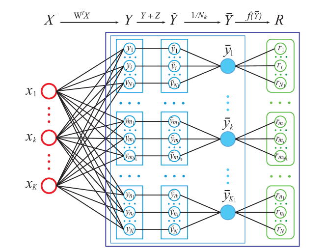
Figure 1: A neural network interpretaton for random variables $X$, $Y$, $\breve{Y}$,$\bar{Y}$, $R$.

A major advantage of incorporating membrane noise is that it facilitates finding the optimal solution by using the infomax principle. Moreover, the optimal solution obtained this way is more robust; that is, it discourages overfitting and has a strong ability to resist distortion. With vanishing noise $\sigma^{2}\rightarrow 0$, we have $\bar{Y}_{k}\rightarrow Y_{k}$, $\tilde{f}(\bar{y}_{k};{\boldsymbol{\tilde{\theta}}}_{k})\simeq\tilde{f}(y_{k};{\boldsymbol{\tilde{\theta}}}_{k})=f(\mathbf{x};{\boldsymbol{\theta}}_{k})$, so that Eqs. (13) and (14) hold as in the case of large $N_{k}$.

To optimize MI $I(Y;R)$, the probability distribution of random variable $Y$, $p(\mathbf{y})$, needs to be determined, i.e. maximizing $I(Y;R)$ about $p(\mathbf{y})$ under some constraints should yield an optimal distribution: $p^{\ast}(\mathbf{y})=\arg\max_{p(\mathbf{y})}I(Y;R)$. Let $\mathcal{C}=\max_{p(\mathbf{y})}I\left(Y;R\right)$ be the channel capacity of neural population coding, and we always have $I(X;R)\leq\mathcal{C}$ (Huang & Zhang,, 2016). To find a suitable linear transformation from $X$ to $Y$ that is compatible with this distribution $p^{\ast}(\mathbf{y})$, a reasonable choice is to maximize $I(X;\breve{Y})$ $\left(\leq I(X;Y)\right)$, where $\breve{Y}$ is a noise-corrupted version of $Y$. This implies minimum information loss in the first transformation step. However, there may exist many transformations from $X$ to $\breve{Y}$ that maximize $I(X;\breve{Y})$ (see Appendix A.3.1). Ideally, if we can find a transformation that maximizes both $I(X;\breve{Y})$ and $I(Y;R)$ simultaneously, then $I(X;R)$ reaches its maximum value: $I(X;R)=\max_{p(\mathbf{y})}I\left(Y;R\right)=\mathcal{C}$.

From the discussion above we see that maximizing $I(X;R)$ can be divided into two steps, namely, maximizing $I(X;\breve{Y})$ and maximizing $I(Y;R)$. The optimal solutions of $\max I(X;\breve{Y})$ and $\max I(Y;R)$ will provide a good initial approximation that tend to be very close to the optimal solution of $\max I(X;R)$.

Similarly, we can extend this method to multilayer neural population networks. For example, a two-layer network with outputs $R^{(1)}$ and $R^{(2)}$ form a Markov chain, $X\rightarrow\tilde{R}^{(1)}\rightarrow R^{(1)}\rightarrow\bar{R}^{(1)}\rightarrow R^{(2)}$, where random variable $\tilde{R}^{(1)}$ is similar to $Y$, random variable $R^{(1)}$ is similar to $\breve{Y}$, and $\bar{R}^{(1)}$ is similar to $\bar{Y}$ in the above. Then we can show that the optimal solution of $\max I(X;R^{(2)})$ can be approximated by the solutions of $\max I(X;R^{(1)})$ and $\max I(\tilde{R}^{(1)};R^{(2)})$, with $I(\tilde{R}^{(1)};R^{(2)})\simeq I(\bar{R}^{(1)};R^{(2)})$.

More generally, consider a highly nonlinear feedforward neural network that maps the input $\mathbf{x}$ to output $\mathbf{z}$, with $\mathbf{z}=F(\mathbf{x;}{\boldsymbol{\theta}})=h_{L}\circ\cdots\circ h_{1}\left(\mathbf{x}\right)$, where $h_{l}$ ($l=1,\cdots,L$) is a linear or nonlinear function (Montufar et al.,, 2014). We aim to find the optimal parameter ${\boldsymbol{\theta}}$ by maximizing $I\left(X;Z\right)$. It is usually difficult to solve the optimization problem when there are many local extrema for $F(\mathbf{x;}{\boldsymbol{\theta}})$. However, if each function $h_{l}$ is easy to optimize, then we can use the hierarchical infomax method described above to get a good initial approximation to its global optimization solution, and go from there to find the final optimal solution. This information-theoretic consideration from the neural population coding point of view may help explain why deep structure networks with unsupervised pre-training have a powerful ability for learning representations.

2.3 The Objective Function

The optimization processes for maximizing $I(X;\breve{Y})$ and maximizing $I(Y;R)$ are discussed in detail in Appendix A.3. First, by maximizing $I(X;\breve{Y})$ (see Appendix A.3.1 for details), we can get the optimal weight parameter $\mathbf{w}_{k}$ ($k=1,\cdots,K_{1}$, see Eq. 7) and its population density $\alpha_{k}$ (see Eq. 6) which satisfy

$$\mathbf{W}={\left[\mathbf{w}_{1},\cdots,\mathbf{w}_{K_{1}}\right]}={a}\mathbf{U}_{0}{\boldsymbol{\Sigma}_{0}^{-1/2}\mathbf{C}}\text{,}$$ (15)

$$\alpha_{1}=\cdots=\alpha_{K_{1}}=K_{1}^{-1}\text{,}$$ (16)

where $a=\sqrt{{K_{1}}K_{0}^{-1}}$, ${\mathbf{C}}=[\mathbf{c}_{1},\cdots,\mathbf{c}_{K_{1}}]\in\mathbb{R}^{K_{0}\times K_{1}}$, ${\mathbf{CC}}^{T}=\mathbf{I}_{K_{0}}$, $\mathbf{I}_{K_{0}}$ is a $K_{0}\times K_{0}$ identity matrix with integer $K_{0}\in\left[1,K\right]$, the diagonal matrix $\mathbf{\Sigma}_{0}\in\mathbb{R}^{K_{0}\times K_{0}}$ and matrix $\mathbf{U}_{0}\in\mathbb{R}^{K\times K_{0}}$ are given in (A.44) and (A.45), with $K_{0}$ given by Eq. (A.52). Matrices $\mathbf{\Sigma}_{0}$ and $\mathbf{U}_{0}$ can be obtained by $\mathbf{\Sigma}$ and $\mathbf{U}$ with $\mathbf{U}_{0}^{T}\mathbf{U}_{0}=\mathbf{I}_{K_{0}}$ and $\mathbf{U}_{0}\mathbf{\mathbf{\Sigma}}_{0}\mathbf{U}_{0}^{T}\approx\mathbf{U\mathbf{\Sigma}U}^{T}\approx\left\langle\mathbf{xx}^{T}\right\rangle_{\mathbf{x}}$ (see Eq. A.23). The optimal weight parameter $\mathbf{w}_{k}$ (15) means that the input variable $\mathbf{x}$ must first undergo a whitening-like transformation $\mathbf{\hat{x}}=\mathbf{\Sigma}_{0}^{-1/2}\mathbf{U}_{0}^{T}\mathbf{x}$, and then goes through the transformation $\mathbf{y}=a{\mathbf{C}}^{T}\mathbf{\hat{x}}$, with matrix ${\mathbf{C}}$ to be optimized below. Note that weight matrix $\mathbf{W}$ satisfies $\mathrm{rank}(\mathbf{W})=\min(K_{0},K_{1})$, which is a low rank matrix, and its low dimensionality helps reduce overfitting during training (see Appendix A.3.1).

By maximizing $I\left(Y;R\right)$ (see Appendix A.3.2), we further solve the the optimal parameters ${\boldsymbol{\tilde{\theta}}}_{k}$ for the nonlinear functions $\tilde{f}(y_{k};{\boldsymbol{\tilde{\theta}}}_{k})$, $k=1,\cdots,K_{1}$. Finally, the objective function for our optimization problem (Eqs. 5 and 6) turns into (see Appendix A.3.3 for details):

$$\mathsf{minimize}\;\;{Q\left[{\mathbf{C}}\right]=}-\frac{1}{2}\left\langle\ln\left(\det\left({\mathbf{C\boldsymbol{\hat{\Phi}}C}}^{T}\right)\right)\right\rangle_{\mathbf{\hat{x}}}\text{,}$$ (17)

$$\mathsf{subject\;to}\;{\mathbf{CC}}^{T}=\mathbf{I}_{K_{0}}\text{,}$$ (18)

where $\boldsymbol{\hat{\Phi}}={{\mathrm{diag}}}\left(\phi(\hat{y}_{1})^{2},\cdots,\phi(\hat{y}_{K_{1}})^{2}\right)$, $\phi(\hat{y}_{k})=a^{-1}\left|\partial g_{k}(\hat{y}_{k})/\partial\hat{y}_{k}\right|$ ($k=1,\cdots,K_{1}$), $g_{k}(\hat{y}_{k})=2\sqrt{\tilde{f}(\hat{y}_{k};{\boldsymbol{\tilde{\theta}}}_{k})}$, $\hat{y}_{k}=a^{-1}y_{k}=\mathbf{c}_{k}^{T}\mathbf{\hat{x}}$, and $\mathbf{\hat{x}}=\mathbf{\Sigma}_{0}^{-1/2}\mathbf{U}_{0}^{T}\mathbf{x}$. We apply the gradient descent method to optimize the objective function, with the gradient of $Q{\left[{\mathbf{C}}\right]}$ given by:

$$\frac{dQ{\left[{\mathbf{C}}\right]}}{d{\mathbf{C}}}=-\left\langle\left({\mathbf{C\boldsymbol{\hat{\Phi}}C}}^{T}\right)^{-1}\mathbf{C}\boldsymbol{\hat{\Phi}}+\mathbf{\hat{x}}\boldsymbol{\omega}^{T}\right\rangle_{\mathbf{\hat{x}}}\text{,}$$ (19)

where $\boldsymbol{\omega}=\left(\omega_{1}{,}\cdots,\omega{{}_{K_{1}}}\right)^{T}$, $\omega_{k}=\phi(\hat{y}_{k})\phi^{\prime}(\hat{y}_{k})\mathbf{c}_{k}^{T}\left({\mathbf{C\boldsymbol{\hat{\Phi}}C}}^{T}\right)^{-1}\mathbf{c}_{k}$, $k=1,\cdots,K_{1}$.

When ${K_{0}}=K_{1}$ (or ${K_{0}}>K_{1}$), the objective function $Q{\left[{\mathbf{C}}\right]}$ can be reduced to a simpler form, and its gradient is also easy to compute (see Appendix A.4.1). However, when ${K_{0}}<K_{1}$, it is computationally expensive to update $\mathbf{C}$ by applying the gradient of $Q{\left[{\mathbf{C}}\right]}$ directly, since it requires matrix inversion for every $\mathbf{\hat{x}}$. We use another objective function $\hat{Q}{\left[{\mathbf{C}}\right]}$ (see Eq. A.118) which is an approximation to $Q{\left[{\mathbf{C}}\right]}$, but its gradient is easier to compute (see Appendix A.4.2). The function $\hat{Q}{\left[{\mathbf{C}}\right]}$ is the approximation of $Q{\left[{\mathbf{C}}\right]}$, ideally they have the same optimal solution for the parameter $\mathbf{C}$.

Usually, for optimizing the objective in Eq. 17, the orthogonality constraint (Eq. 18) is unnecessary. However, this orthogonality constraint can accelerate the convergence rate if we employ it for the initial iteration to update $\mathbf{C}$ (see Appendix A.5).

3 Experimental Results

We have applied our methods to the natural images from Olshausen’s image dataset (Olshausen & Field,, 1996) and the images of handwritten digits from MNIST dataset (LeCun et al.,, 1998) using Matlab 2016a on a computer with 12 Intel CPU cores (2.4 GHz). The gray level of each raw image was normalized to the range of $0$ to $1$. $M\$image patches with size $w\times w=K$ for training were randomly sampled from the images. We used the Poisson neuron model with a modified sigmoidal tuning function $\tilde{f}(y;{\boldsymbol{\tilde{\theta}}})=\frac{1}{4\left(1+\exp\left(-\beta y-b\right)\right)^{2}}$, with $g(y)=2\sqrt{\tilde{f}(y;{\boldsymbol{\tilde{\theta}}})}=\frac{1}{1+\exp\left(-\beta y-b\right)}$, where ${\boldsymbol{\tilde{\theta}}}=\left(\beta,b\right)^{T}$. We obtained the initial values (see Appendix A.3.2): $b_{0}=0$ and $\beta_{0}\approx 1.81\sqrt{{K_{1}}K_{0}^{-1}}$. For our experiments, we set $\beta=0.5\beta_{0}$ for iteration epoch $t=1,\cdots,t_{0}$ and $\beta=\beta_{0}$ for $t=t_{0}+1,\cdots,t_{\max}$, where $t_{0}=50$.

Firstly, we tested the case of $K=K_{0}=K_{1}=144$ and randomly sampled $M=10^{5}$ image patches with size $12\times 12$ from the Olshausen’s natural images, assuming that $N=10^{6}$ neurons were divided into $K_{1}=144$ classes and $\epsilon=1$ (see Eq. A.52 in Appendix). The input patches were preprocessed by the ZCA whitening filters (see Eq. A.68). To test our algorithms, we chose the batch size to be equal to the number of training samples $M$, although we could also choose a smaller batch size. We updated the matrix $\mathbf{C}$ from a random start, and set parameters $t_{\max}=300$, ${v}_{1}=0.4$, and $\tau=0.8$ for all experiments.

In this case, the optimal solution $\mathbf{C}$ looked similar to the optimal solution of IICA (Bell & Sejnowski,, 1997). We also compared with the fast ICA algorithm (FICA) (Hyvärinen,, 1999), which is faster than IICA. We also tested the restricted Boltzmann machine (RBM) (Hinton et al.,, 2006) for a unsupervised learning of representations, and found that it could not easily learn Gabor-like filters from Olshausen’s image dataset as trained by contrastive divergence. However, an improved method by adding a sparsity constraint on the output units, e.g., sparse RBM (SRBM) (Lee et al.,, 2008) or sparse autoencoder (Hinton,, 2010), could attain Gabor-like filters from this dataset. Similar results with Gabor-like filters were also reproduced by the denoising autoencoders (Vincent et al.,, 2010), which method requires a careful choice of parameters, such as noise level, learning rate, and batch size.

In order to compare our methods, i.e. Algorithm 1 (Alg.1, see Appendix A.4.1) and Algorithm 2 (Alg.2, see Appendix A.4.2), with other methods, i.e. IICA, FICA and SRBM, we implemented these algorithms using the same initial weights and the same training data set (i.e. $10^{5}$ image patches preprocessed by the ZCA whitening filters). To get a good result by IICA, we must carefully select the parameters; we set the batch size as $50$, the initial learning rate as $0.01$, and final learning rate as $0.0001$, with an exponential decay with the epoch of iterations. IICA tends to have a faster convergence rate for a bigger batch size but it may become harder to escape local minima. For FICA, we chose the nonlinearity function $f(u)=\log\cosh(u)$ as contrast function, and for SRBM, we set the sparseness control constant $p$ as $0.01$ and $0.03$. The number of epoches for iterations was set to $300$ for all algorithms. Figure 2 shows the filters learned by our methods and other methods. Each filter in Figure 2 corresponds to a column vector of matrix ${\mathbf{\check{C}}}$ (see Eq. A.69), where each vector for display is normalized by $\mathbf{\check{c}}_{k}\leftarrow\mathbf{\check{c}}_{k}/\max(|\check{c}_{1,k}|,\cdots,|\check{c}_{K,k}|)$, $k=1,\cdots,K_{1}$. The results in Figures 2, 2 and 2 look very similar to one another, and slightly different from the results in Figure 2 and 2. There are no Gabor-like filters in Figure 2, which corresponds to SRBM with $p=0.03$.

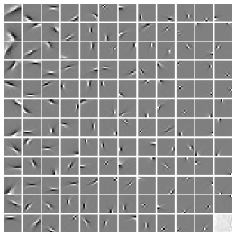
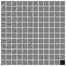
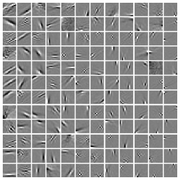
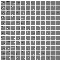
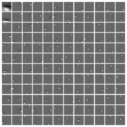
Figure 2: Comparison of filters obtained from ${10^{5}}$ natural image patches of size 12$\times$12 by our methods (Alg.1 and Alg.2) and other methods. The number of output filters was $K_{1}=144$. (a): Alg.1. (b): Alg.2. (c): IICA. (d): FICA. (e): SRBM ($p=0.01$). (f): SRBM ($p=0.03$).

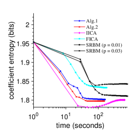
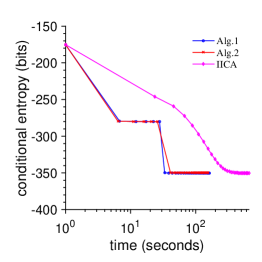
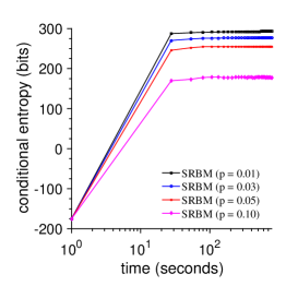
Figure 3: Comparison of quantization effects and convergence rate by coefficient entropy (see A.122) and conditional entropy (see A.125) corresponding to training results (filters) shown in Figure 2. The coefficient entropy (panel a) and conditional entropy (panel b and c) are shown as a function of training time on a logarithmic scale. All experiments run on the same machine using Matlab. Here we sampled once every $10$ epoches out of a total of $300$ epoches. We set epoch number $t_{0}=50$ for Alg.1 and Alg.2 and the start time to $1$ second.

Figure 3 shows how the coefficient entropy (CFE) (see Eq. A.122) and the conditional entropy (CDE) (see Eq. A.125) varied with training time. We calculated CFE and CDE by sampling once every $10$ epoches from a total of $300$ epoches. These results show that our algorithms had a fast convergence rate towards stable solutions while having CFE and CDE values similar to the algorithm of IICA, which converged much more slowly. Here the values of CFE and CDE should be as small as possible for a good representation learned from the same data set. Here we set epoch number $t_{0}=50$ in our algorithms (see Alg.1 and Alg.2), and the start time was set to $1$ second. This explains the step seen in Figure 3 (b) for Alg.1 and Alg.2 since the parameter $\beta$ was updated when epoch number $t=t_{0}$. FICA had a convergence rate close to our algorithms but had a big CFE, which is reflected by the quality of the filter results in Figure 2. The convergence rate and CFE for SRBM were close to IICA, but SRBM had a much bigger CDE than IICA, which implies that the information had a greater loss when passing through the system optimized by SRBM than by IICA or our methods.

From Figure 3 we see that the CDE (or MI $I(X;R)$, see Eq. A.124 and A.125) decreases (or increases) with the increase of the value of the sparseness control constant $p$. Note that a smaller $p$ means sparser outputs. Hence, in this sense, increasing sparsity may result in sacrificing some information. On the other hand, a weak sparsity constraint may lead to failure of learning Gabor-like filters (see Figure 2), and increasing sparsity has an advantage in reducing the impact of noise in many practical cases. Similar situation also occurs in sparse coding (Olshausen & Field,, 1997), which provides a class of algorithms for learning overcomplete dictionary representations of the input signals. However, its training is time consuming due to its expensive computational cost, although many new training algorithms have emerged (e.g. Aharon et al.,, 2006; Elad & Aharon,, 2006; Lee et al.,, 2006; Mairal et al.,, 2010). See Appendix A.5 for additional experimental results.

4 Conclusions

In this paper, we have presented a framework for unsupervised learning of representations via information maximization for neural populations. Information theory is a powerful tool for machine learning and it also provides a benchmark of optimization principle for neural information processing in nervous systems. Our framework is based on an asymptotic approximation to MI for a large-scale neural population. To optimize the infomax objective, we first use hierarchical infomax to obtain a good approximation to the global optimal solution. Analytical solutions of the hierarchical infomax are further improved by a fast convergence algorithm based on gradient descent. This method allows us to optimize highly nonlinear neural networks via hierarchical optimization using infomax principle.

From the viewpoint of information theory, the unsupervised pre-training for deep learning (Hinton & Salakhutdinov,, 2006; Bengio et al.,, 2007) may be reinterpreted as a process of hierarchical infomax, which might help explain why unsupervised pre-training helps deep learning (Erhan et al.,, 2010). In our framework, a pre-whitening step can emerge naturally by the hierarchical infomax, which might also explain why a pre-whitening step is useful for training in many learning algorithms (Coates et al.,, 2011; Bengio,, 2012).

Our model naturally incorporates a considerable degree of biological realism. It allows the optimization of a large-scale neural population with noisy spiking neurons while taking into account of multiple biological constraints, such as membrane noise, limited energy, and bounded connection weights. We employ a technique to attain a low-rank weight matrix for optimization, so as to reduce the influence of noise and discourage overfitting during training. In our model, many parameters are optimized, including the population density of parameters, filter weight vectors, and parameters for nonlinear tuning functions. Optimizing all these model parameters could not be easily done by many other methods.

Our experimental results suggest that our method for unsupervised learning of representations has obvious advantages in its training speed and robustness over the main existing methods. Our model has a nonlinear feedforward structure and is convenient for fast learning and inference. This simple and flexible framework for unsupervised learning of presentations should be readily extended to training deep structure networks. In future work, it would interesting to use our method to train deep structure networks with either unsupervised or supervised learning.

Appendix

A.1 Formulas for Approximation of Mutual Information

It follows from $I(X;R)=\left\langle\ln\frac{p(\mathbf{x}|\mathbf{r})}{p(\mathbf{x})}\right\rangle_{\mathbf{r},\mathbf{x}}$ and Eq. (1) that the conditional entropy should read:

$$H(X|R)=-\left\langle\ln p(\mathbf{x}|\mathbf{r})\right\rangle_{\mathbf{r},\mathbf{x}}\simeq-\frac{1}{2}\left\langle\ln\left(\det\left(\frac{\mathbf{G}(\mathbf{x})}{2\pi e}\right)\right)\right\rangle_{\mathbf{x}}\text{.}$$ (A.1)

The Fisher information matrix $\mathbf{J}(\mathbf{x})$ (see Eq. 3), which is symmetric and positive semidefinite, can be written also as

$$\mathbf{J}(\mathbf{x})=\left\langle\frac{\partial\ln p(\mathbf{r}|\mathbf{x})}{\partial\mathbf{x}}\frac{\partial\ln p(\mathbf{r}|\mathbf{x})}{\partial\mathbf{x}^{T}}\right\rangle_{\mathbf{r}|\mathbf{x}}\text{.}$$ (A.2)

If we suppose $p(\mathbf{r}|\mathbf{x})$ is conditional independent, namely, $p(\mathbf{r}|\mathbf{x})=\prod_{n=1}^{N}p(r_{n}|\mathbf{x};\boldsymbol{\theta}_{n})$, then we have (see Huang & Zhang,, 2016)

$$\mathbf{J}(\mathbf{x})=N\int_{{\Theta}}p({\boldsymbol{\theta}})\mathbf{S}(\mathbf{x};{\boldsymbol{\theta}})d{\boldsymbol{\theta}}\text{,}$$ (A.3)

$$\mathbf{S}(\mathbf{x};\boldsymbol{\theta})=\left\langle\frac{\partial\ln p(r|\mathbf{x};\boldsymbol{\theta})}{\partial\mathbf{x}}\frac{\partial\ln p(r|\mathbf{x};\boldsymbol{\theta})}{\partial\mathbf{x}^{T}}\right\rangle_{r|\mathbf{x}}\text{,}$$ (A.4)

where $p(\boldsymbol{\theta})$ is the population density function of parameter ${\boldsymbol{\theta}}$,

$$p(\boldsymbol{\theta})=\frac{1}{N}\sum_{n=1}^{N}\delta(\boldsymbol{\theta}-\boldsymbol{\theta}_{n})\text{,}$$ (A.5)

and $\delta(\cdot)$ denotes the Dirac delta function. It can be proved that the approximation function of MI $I_{G}[p({\boldsymbol{\theta}})]$ (Eq. 1) is concave about $p({\boldsymbol{\theta}})$ (Huang & Zhang,, 2016). In Eq. (A.3), we can approximate the continuous integral by a discrete summation for numerical computation,

$$\mathbf{J}(\mathbf{x})\approx N\sum_{k=1}^{K_{1}}\alpha_{k}\mathbf{S}(\mathbf{x};{\boldsymbol{\theta}}_{k})\text{,}$$ (A.6)

where $\sum_{k=1}^{K_{1}}\alpha_{k}=1$, $\alpha_{k}>0$, $k=1,\cdots,K_{1}$, $1\leq K_{1}\leq N$.

For Poisson neuron model, by Eq. (A.4) we have (see Huang & Zhang,, 2016)

$${p(r|\mathbf{x}};{{\boldsymbol{\theta}})} ={\dfrac{f(\mathbf{x};{\boldsymbol{\theta}})^{r}}{r!}\exp\left(-f(\mathbf{x};{\boldsymbol{\theta}})\right)}\text{,}$$ (A.7)

$${\mathbf{S}(\mathbf{x}};{{\boldsymbol{\theta}})} ={\dfrac{1}{f(\mathbf{x};{\boldsymbol{\theta}})}\dfrac{\partial f(\mathbf{x};{\boldsymbol{\theta}})}{\partial\mathbf{x}}\dfrac{\partial f(\mathbf{x};{\boldsymbol{\theta}})}{\partial\mathbf{x}^{T}}}$$

$$={\dfrac{\partial g(\mathbf{x};{\boldsymbol{\theta}})}{\partial\mathbf{x}}\dfrac{\partial g(\mathbf{x};{\boldsymbol{\theta}})}{\partial\mathbf{x}^{T}}}\text{,}$$ (A.8)

where $f(\mathbf{x};{\boldsymbol{\theta}})\geq 0$ is the activation function (mean response) of neuron and

$${g(\mathbf{x}};{{\boldsymbol{\theta}})}=2\sqrt{f(\mathbf{x};{\boldsymbol{\theta}})}\text{.}$$ (A.9)

Similarly, for Gaussian noise model, we have

$${p(r|\mathbf{x}};{{\boldsymbol{\theta}})}={\dfrac{1}{\sigma\sqrt{2\pi}}\exp\left(-\dfrac{\left(r-f(\mathbf{x};{\boldsymbol{\theta}})\right)^{2}}{2\sigma^{2}}\right)}\text{,}$$ (A.10)

$${\mathbf{S}(\mathbf{x}};{{\boldsymbol{\theta}})}={\dfrac{1}{\sigma^{2}}\dfrac{\partial f(\mathbf{x};{\boldsymbol{\theta}})}{\partial\mathbf{x}}\dfrac{\partial f(\mathbf{x};{\boldsymbol{\theta}})}{\partial\mathbf{x}^{T}}}\text{,}$$ (A.11)

where $\sigma>0$ denotes the standard deviation of noise.

Sometimes we do not know the specific form of $p(\mathbf{x})$ and only know $M$ samples, $\mathbf{x}_{1}$, $\cdots$, $\mathbf{x}_{M}$, which are independent and identically distributed (i.i.d.) samples drawn from the distribution $p(\mathbf{x})$. Then we can use the empirical average to approximate the integral in Eq. (1):

$$I_{G}\approx\frac{1}{2}\sum_{m=1}^{M}\ln\left(\det\left(\mathbf{G}(\mathbf{x}_{m})\right)\right)+H\left(X\right)\text{.}$$ (A.12)

A.2 Proof of Proposition 1

Proof. It follows from the data-processing inequality (Cover & Thomas,, 2006) that

$$I(X;R) \leq I(Y;R)\leq I(\breve{Y};R)\leq I(\bar{Y};R)\text{, }$$ (A.13)

$$I(X;R) \leq I(X;\bar{Y})\leq I(X;\breve{Y})\leq I(X;Y)\text{.}$$ (A.14)

Since

$${p(\bar{y}_{k}|\mathbf{x}{)}}=p({\breve{y}_{k_{1}},\cdots,\breve{y}_{k_{N_{k}}}}|\mathbf{x)}={\mathcal{N}(\mathbf{w}_{k}^{T}\mathbf{x},\,N_{k}^{-1}\sigma^{2})}\text{, }k=1,\cdots,K_{1}\text{,}$$ (A.15)

we have

$${p(\mathbf{\bar{y}}|\mathbf{x}{)}}=p(\mathbf{\breve{y}}|\mathbf{x)}\text{,}$$ (A.16)

$${p(\mathbf{\bar{y}}{)}}=p(\mathbf{\breve{y})}\text{,}$$ (A.17)

$$I(X;\bar{Y})=I(X;\breve{Y})\text{.}$$ (A.18)

Hence, by (A.14) and (A.18), expression (12) holds.

On the other hand, when $N_{k}$ is large, from Eq. (10) we know that the distribution of $\bar{Z}_{k}$, namely, ${\mathcal{N}\left(0\text{,\thinspace}N_{k}^{-1}\sigma^{2}\right)}$,  approaches a Dirac delta function $\delta(\bar{z}_{k})$. Then by (7) and (9) we have $p\left(\mathbf{r}|\mathbf{\bar{y}}\right)\simeq{p(\mathbf{r}|}$$\mathbf{y}$${{)}}=p\left(\mathbf{r}|\mathbf{x}\right)$ and

$$I(X;R) =I\left(Y;R\right)-\left\langle\ln\frac{p\left(\mathbf{r}|\mathbf{y}\right)}{p\left(\mathbf{r}|\mathbf{x}\right)}\right\rangle_{\mathbf{r},\mathbf{x}}=I\left(Y;R\right)\text{,}$$ (A.19)

$$I\left(Y;R\right) =I(\bar{Y};R)-\left\langle\ln\frac{p\left(\mathbf{r}|\mathbf{\bar{y}}\right)}{p\left(\mathbf{r}|\mathbf{y}\right)}\right\rangle_{\mathbf{r},\mathbf{y},\mathbf{\bar{y}}}\simeq I(\bar{Y};R)\text{,}$$ (A.20)

$$I\left(Y;R\right) =I(\breve{Y};R)-\left\langle\ln\frac{p\left(\mathbf{r}|\mathbf{\breve{y}}\right)}{p\left(\mathbf{r}|\mathbf{y}\right)}\right\rangle_{\mathbf{r},\mathbf{y},\mathbf{\breve{y}}}\simeq I(\breve{Y};R)\text{,}$$ (A.21)

$$I(X;Y) =I(X;\bar{Y})-\left\langle\ln\frac{p\left(\mathbf{x}|\mathbf{\bar{y}}\right)}{p\left(\mathbf{x}|\mathbf{y}\right)}\right\rangle_{\mathbf{x},\mathbf{y},\mathbf{\bar{y}}}\simeq I(X;\bar{Y})\text{.}$$ (A.22)

It follows from (A.13) and (A.19) that (11) holds. Combining (11), (12) and (A.20)–(A.22),  we immediately get (13) and (14). This completes the proof of Proposition 1. $\Box$

A.3 Hierarchical Optimization for Maximizing $I(X;R)$

In the following, we will discuss the optimization procedure for maximizing $I(X;R)$ in two stages: maximizing $I(X;\breve{Y})$ and maximizing $I(Y;R)$.

A.3.1 The 1st Stage

In the first stage, our goal is to maximize the MI $I(X;\breve{Y})$ and get the optimal parameters $\mathbf{w}_{k}$ ($k=1,\cdots,K_{1}$). Assume that the stimulus $\mathbf{x}$ has zero mean (if not, let $\mathbf{x}\leftarrow\mathbf{x}-\left\langle\mathbf{x}\right\rangle_{\mathbf{x}}$) and covariance matrix $\boldsymbol{\Sigma}_{\mathbf{x}}$. It follows from eigendecomposition that

$$\boldsymbol{\Sigma}_{\mathbf{x}}=\left\langle\mathbf{xx}^{T}\right\rangle_{\mathbf{x}}\approx\frac{1}{M-1}\mathbf{XX}^{T}=\mathbf{U}\boldsymbol{\Sigma}\mathbf{U}^{T}\text{,}$$ (A.23)

where $\mathbf{X}=[\mathbf{x}_{1}$, $\cdots$, $\mathbf{x}_{M}]$, $\mathbf{U}=[\mathbf{u}_{1},\cdots,\mathbf{u}_{K}]\in\mathbb{R}^{K\times K}$ is an unitary orthogonal matrix and $\boldsymbol{\Sigma}={\mathrm{diag}}\left(\sigma_{1}^{2},\cdots,\sigma_{K}^{2}\right)$ is a positive diagonal matrix with $\sigma_{1}\geq\cdots\geq\sigma_{K}>0$. Define

$$\mathbf{\tilde{x}}=\boldsymbol{\Sigma}^{-1/2}\mathbf{U}^{T}\mathbf{x}\text{,}$$ (A.24)

$$\mathbf{\tilde{w}}_{k}=\boldsymbol{\Sigma}{{}^{1/2}\mathbf{U}^{T}}\mathbf{w}_{k}\text{,}$$ (A.25)

$$y_{k}=\mathbf{\tilde{w}}_{k}^{T}\mathbf{\tilde{x}}\text{,}$$ (A.26)

where $k=1,\cdots,K_{1}$. The covariance matrix of $\mathbf{\tilde{x}}$ is given by

$$\boldsymbol{\Sigma}_{\mathbf{\tilde{x}}}=\left\langle\mathbf{\tilde{x}\tilde{x}}^{T}\right\rangle_{\mathbf{\tilde{x}}}\approx\mathbf{I}_{K}\text{,}$$ (A.27)

and $\mathbf{I}_{K}$ is a $K\times K$ identity matrix. From (1) and (A.11) we have $I(X;\breve{Y})=I(\tilde{X};\breve{Y})$ and

$$I(\tilde{X};\breve{Y})\simeq I_{G}^{\prime}=\frac{1}{2}\ln\left(\det\left(\frac{\mathbf{\tilde{G}}}{2\pi e}\right)\right)+H(\tilde{X})\text{,}$$ (A.28)

$$\mathbf{\tilde{G}}\approx{N\sigma^{-2}\sum_{k=1}^{K_{1}}\alpha_{k}}\mathbf{\tilde{w}}_{k}\mathbf{\tilde{w}}_{k}^{T}+\mathbf{I}_{K}\text{.}$$ (A.29)

The following approximations are useful (see Huang & Zhang,, 2016):

$$p(\mathbf{\tilde{x}}) \approx{\mathcal{N}\left(0,\mathbf{I}_{K}\right)}\text{, }$$ (A.30)

$$\mathbf{P}(\mathbf{\tilde{x}}) =-\frac{\partial^{2}\ln p\left(\mathbf{\tilde{x}}\right)}{\partial\mathbf{\tilde{x}}\partial\mathbf{\tilde{x}}^{T}}\approx\mathbf{I}_{K}\text{.}$$ (A.31)

By the central limit theorem, the distribution of random variable $\tilde{X}$ is closer to a normal distribution than the distribution of the original random variable $X$. On the other hand, the PCA models assume multivariate gaussian data whereas the ICA models assume multivariate non-gaussian data. Hence by a PCA-like whitening transformation (A.24) we can use the approximation (A.31) with the Laplace’s method of asymptotic expansion, which only requires that the peak be close to its mean while random variable $\tilde{X}$ needs not be exactly Gaussian.

Without any constraints on the Gaussian channel of neural populations, especially the peak firing rates, the capacity of this channel may grow indefinitely: $I(\tilde{X};\breve{Y})\rightarrow\infty$. The most common constraint on the neural populations is an energy or power constraint which can also be regarded as a signal-to-noise ratio (SNR) constraint. The SNR for the output $\breve{y}_{n}$ of the n-th neuron is given by

$$\mathrm{SNR}_{n}=\frac{1}{\sigma^{2}}\left\langle\left(\mathbf{w}_{n}^{T}\mathbf{x}\right)^{2}\right\rangle_{\mathbf{x}}\approx\frac{1}{\sigma^{2}}\mathbf{\tilde{w}}_{n}^{T}\mathbf{\tilde{w}}_{n}\text{, }n=1,\cdots,N\text{.}$$ (A.32)

We require that

$$\frac{1}{N}{\sum_{n=1}^{N}}\mathrm{SNR}_{n}\approx\frac{1}{\sigma^{2}}{\sum_{k=1}^{K_{1}}\alpha_{k}}\mathbf{\tilde{w}}_{k}^{T}\mathbf{\tilde{w}}_{k}\leq\rho\text{,}$$ (A.33)

where $\rho$ is a positive constant. Then by Eq. (A.28), (A.29) and (A.33), we have the following optimization problem:

$$\mathsf{minimize}\mathrm{\;}{Q_{G}^{\prime}[\mathbf{\hat{W}}]}=-\frac{1}{2}{\ln\left(\det\left(N\sigma^{-2}\mathbf{\hat{W}\hat{W}}^{T}+\mathbf{I}_{K}\right)\right)}\text{,}$$ (A.34)

$$\mathsf{subject\;to\;}{h}=\mathrm{Tr}\left(\mathbf{\hat{W}\hat{W}}^{T}\right)-E\leq 0\text{,}$$ (A.35)

where $\mathrm{Tr}\left(\cdot\right)$ denotes matrix trace and

$$\mathbf{\hat{W}}=\mathbf{\tilde{W}A}^{1/2}={\boldsymbol{\Sigma}^{1/2}\mathbf{U}^{T}}\mathbf{WA}^{1/2}={\left[\mathbf{\hat{w}}_{1},\cdots,\mathbf{\hat{w}}_{K_{1}}\right]}\text{,}$$ (A.36)

$${\mathbf{A}}={\mathrm{diag}\left(\alpha_{1},\cdots,\alpha_{K_{1}}\right)}\text{,}$$ (A.37)

$$\mathbf{W}={\left[\mathbf{w}_{1},\cdots,\mathbf{w}_{K_{1}}\right]}\text{,}$$ (A.38)

$$\mathbf{\tilde{W}}={\left[\mathbf{\tilde{w}}_{1},\cdots,\mathbf{\tilde{w}}_{K_{1}}\right]}\text{,}$$ (A.39)

$$E=\rho\sigma^{2}\text{.}$$ (A.40)

Here $E$ is a constant that does not affect the final optimal solution so we set $E=1$. Then we obtain an optimal solution as follows:

$$\mathbf{W} ={a}\mathbf{U}_{0}{\boldsymbol{\Sigma}_{0}^{-1/2}\mathbf{V}_{0}^{T}}\text{, }$$ (A.41)

$$\mathbf{A} =K_{1}^{-1}{\mathbf{I}}_{K_{1}}\text{, }$$ (A.42)

$$a =\sqrt{E{K_{1}}K_{0}^{-1}}=\sqrt{{K_{1}}K_{0}^{-1}}\text{,}$$ (A.43)

$$\boldsymbol{\Sigma}_{0} ={\mathrm{diag}}\left(\sigma_{1}^{2},\cdots,\sigma_{K_{0}}^{2}\right)\text{,}$$ (A.44)

$$\mathbf{U}_{0} =\mathbf{U}\left(\text{:},1\text{:}K_{0}\right)\in\mathbb{R}^{K\times K_{0}}\text{,}$$ (A.45)

$$\mathbf{V}_{0} =\mathbf{V}\left(\text{:},1\text{:}K_{0}\right)\in\mathbb{R}^{K_{1}\times K_{0}}\text{,}$$ (A.46)

where $\mathbf{V}=[\mathbf{v}_{1},\cdots,\mathbf{v}_{K_{1}}]$ is an $K_{1}\times K_{1}$ unitary orthogonal matrix, parameter $K_{0}$ represents the size of the reduced dimension ($1\leq K_{0}\leq K$), and its value will be determined below. Now the optimal parameters $\mathbf{w}_{n}$ ($n=1,\cdots,N$) are clustered into $K_{1}$ classes (see Eq. A.6) and obey an uniform discrete distribution (see also Eq. A.60 in Appendix A.3.2).

When ${K}=K_{0}={K}_{1}$, the optimal solution of $\mathbf{W}$ in Eq. (A.41) is a whitening-like filter. When ${\mathbf{V=I}}_{K}$, the optimal matrix $\mathbf{W}$ is the principal component analysis (PCA) whitening filters. In the symmetrical case with ${\mathbf{V=U}}$, the optimal matrix $\mathbf{W}$ becomes a zero component analysis (ZCA) whitening filter. If $K<{K}_{1}$, this case leads to an overcomplete solution, whereas when $K_{0}\leq{K}_{1}<K$, the undercomplete solution arises. Since $K_{0}\leq K_{1}$ and $K_{0}\leq K$,$\ {Q_{G}^{\prime}}$ achieves its minimum when $K_{0}=K$. However, in practice other factors may prevent it from reaching this minimum. For example, consider the average of squared weights,

$$\varsigma={\sum_{k=1}^{K_{1}}\alpha_{k}}\left\|\mathbf{w}_{k}\right\|^{2}=\mathrm{Tr}\left(\mathbf{WAW}^{T}\right)=\frac{E}{K_{0}}\sum_{k=1}^{K_{0}}{\sigma_{k}^{-2}}\text{,}$$ (A.47)

where $\left\|\mathbf{\cdot}\right\|$ denotes the Frobenius norm. The value of $\varsigma$ is extremely large when any ${\sigma_{k}\ }$becomes vanishingly small. For real neurons these weights of connection are not allowed to be too large. Hence we impose a limitation on the weights: $\varsigma\leq E_{1}$, where $E_{1}$ is a positive constant. This yields another constraint on the objective function,

$$\tilde{h}=\frac{E}{K_{0}}\sum_{k=1}^{K_{0}}{\sigma_{k}^{-2}-E_{1}\leq 0}\text{.}$$ (A.48)

From (A.35) and (A.48) we get the optimal $K_{0}=\arg\max_{\tilde{K}_{0}}\left(E\tilde{K}_{0}^{-1}\sum_{k=1}^{\tilde{K}_{0}}{\sigma_{k}^{-2}}\right)$. By this constraint, small values of ${\sigma_{k}^{2}}$ will often result in $K_{0}<K$ and a low-rank matrix $\mathbf{W}$ (Eq. A.41).

On the other hand, the low-rank matrix $\mathbf{W}$ can filter out the noise of stimulus $\mathbf{x}$. Consider the transformation $\mathbf{Y}=\mathbf{W}^{T}\mathbf{X}$ with $\mathbf{X}=[\mathbf{x}_{1}$, $\cdots$, $\mathbf{x}_{M}]$ and $\mathbf{Y}=[\mathbf{y}_{1}$,  $\cdots$, $\mathbf{y}_{M}]$ for $M$ samples. It follows from the singular value decomposition (SVD) of $\mathbf{X}$ that

$$\mathbf{X}=\mathbf{US\tilde{V}}^{T}\text{,}$$ (A.49)

where $\mathbf{U}$ is given in (A.23), $\mathbf{\tilde{V}}$ is a $M\times M$ unitary orthogonal matrix, $\mathbf{S}\$is a $K\times M$ diagonal matrix with non-negative real numbers on the diagonal, $S_{k,k}=\sqrt{M-1}\sigma_{k}$ ($k=1,\cdots,K$, $K\leq M$), and $\mathbf{SS}^{T}=(M-1){\boldsymbol{\Sigma}}$. Let

$$\mathbf{\breve{X}}=\sqrt{M-1}\mathbf{U}_{0}{\boldsymbol{\Sigma}}_{0}^{1/2}\mathbf{\tilde{V}}_{0}^{T}\approx\mathbf{X}\text{,}$$ (A.50)

where $\mathbf{\tilde{V}}_{0}=\mathbf{\tilde{V}}\left(\text{:},1\text{:}K_{0}\right)\in\mathbb{R}^{M\times K_{0}}$, ${\boldsymbol{\Sigma}}_{0}$ and $\mathbf{U}_{0}$ are given in (A.44) and (A.45), respectively. Then

$$\mathbf{Y}=\mathbf{W}^{T}\mathbf{X}={a\mathbf{V}_{0}\boldsymbol{\Sigma}_{0}^{-1/2}}\mathbf{U}_{0}^{T}\mathbf{US\tilde{V}}^{T}=\mathbf{W}^{T}\mathbf{\breve{X}}=a\sqrt{M-1}{\mathbf{V}_{0}}\mathbf{\tilde{V}}_{0}^{T}\text{,}$$ (A.51)

where $\mathbf{\breve{X}}$ can be regarded as a denoised version of $\mathbf{X}$. The determination of the effective rank $K_{0}\leq K$ of the matrix $\mathbf{\breve{X}}$ by using singular values is based on various criteria (Konstantinides & Yao,, 1988). Here we choose $K_{0}$ as follows:

$$K_{0}=\arg\min_{K_{0}^{\prime}}\left(\sqrt{\frac{\sum_{k=1}^{K_{0}^{\prime}}{\sigma_{k}^{2}}}{\sum_{k=1}^{K}{\sigma_{k}^{2}}}}\geq\epsilon\right)\text{,}$$ (A.52)

where $\epsilon\$is a positive constant ($0<\epsilon\leq 1$).

Another advantage of a low-rank matrix $\mathbf{W}$ is that it can significantly reduce overfitting for learning neural population parameters. In practice, the constraint (A.47) is equivalent to a weight-decay regularization term used in many other optimization problems (Cortes & Vapnik,, 1995; Hinton,, 2010), which can reduce overfitting to the training data. To prevent the neural networks from overfitting, Srivastava et al., (2014) presented a technique to randomly drop units from the neural network during training, which may in fact be regarded as an attempt to reduce the rank of the weight matrix because the dropout can result in a sparser weights (lower rank matrix). This means that the update is only concerned with keeping the more important components, which is similar to first performing a denoising process by the SVD low rank approximation.

In this stage, we have obtained the optimal parameter $\mathbf{W}$ (see A.41). The optimal value of matrix ${\mathbf{V}_{0}}$ can also be determined, as shown in Appendix A.3.3.

A.3.2 The 2nd Stage

For this stage, our goal is to maximize the MI $I(Y;R)$ and get the optimal parameters ${\boldsymbol{\tilde{\theta}}}_{k}$, $k=1,\cdots,K_{1}$. Here the input is $\mathbf{y}=(y_{1},\cdots,y_{K_{1}})^{T}$ and the output $\mathbf{r}=(r_{1},\cdots,r_{N})^{T}$ is also clustered into $K_{1}$ classes. The responses of $N_{k}$ neurons in the $k$-th subpopulation obey a Poisson distribution with mean $\tilde{f}(\mathbf{e}_{k}^{T}\mathbf{y};{\boldsymbol{\tilde{\theta}}}_{k})$, where $\mathbf{e}_{k}$ is a unit vector with $1$ in the $k$-th element and $y_{k}=\mathbf{e}_{k}^{T}\mathbf{y}$. By (A.24) and (A.26), we have

$$\left\langle y_{k}\right\rangle_{y_{k}}=0\text{, }$$ (A.53)

$$\sigma_{y_{k}}^{2}=\left\langle y_{k}^{2}\right\rangle_{y_{k}}=\left\|\mathbf{\tilde{w}}_{k}\right\|^{2}\text{.}$$ (A.54)

Then for large $N$, by (1)–(4) and (A.30) we can use the following approximation,

$$I(Y;R)\simeq\breve{I}_{F}=\frac{1}{2}\left\langle\ln\left(\det\left(\frac{\mathbf{\breve{J}}(\mathbf{y})}{2\pi e}\right)\right)\right\rangle_{\mathbf{y}}+H(Y)\text{,}$$ (A.55)

where

$$\mathbf{\breve{J}}(\mathbf{y})={{\mathrm{diag}}}\left(N\alpha_{1}\left|g_{1}^{\prime}(y_{1})\right|^{2},\cdots,N\alpha_{K_{1}}\left|g_{K_{1}}^{\prime}(y_{K_{1}})\right|^{2}\right)\text{,}$$ (A.56)

$$g_{k}^{\prime}(y_{k})=\frac{\partial g_{k}(y_{k})}{\partial y_{k}}\text{, }k=1,\cdots,K_{1}\text{,}$$ (A.57)

$$g_{k}(y_{k})=2\sqrt{\tilde{f}(y_{k};{\boldsymbol{\tilde{\theta}}}_{k})}\text{, }k=1,\cdots,K_{1}\text{.}$$ (A.58)

It is easy to get that

$$\breve{I}_{F} =\frac{1}{2}\sum_{k=1}^{K_{1}}\left\langle\ln\left(\frac{N\alpha_{k}\left|g_{k}^{\prime}(y_{k})\right|^{2}}{2\pi e}\right)\right\rangle_{\mathbf{y}}+H(Y)$$

$$\leq\frac{1}{2}\sum_{k=1}^{K_{1}}\left\langle\ln\left(\frac{\left|g_{k}^{\prime}(y_{k})\right|^{2}}{2\pi e}\right)\right\rangle_{\mathbf{y}}-\frac{K_{1}}{2}\ln\left(\frac{K_{1}}{N}\right)+H(Y)\text{,}$$ (A.59)

where the equality holds if and only if

$$\alpha_{k}=\frac{1}{K_{1}},k=1,\cdots,K_{1}\text{,}$$ (A.60)

which is consistent with Eq. (A.42).

On the other hand, it follows from the Jensen’s inequality that

$$\breve{I}_{F} =\left\langle\ln\left(p\left(\mathbf{y}\right)^{-1}\det\left(\frac{\mathbf{\breve{J}}(\mathbf{y})}{2\pi e}\right)^{1/2}\right)\right\rangle_{\mathbf{y}}$$

$$\leq\ln\int\det\left(\dfrac{\mathbf{\breve{J}}(\mathbf{y})}{2\pi e}\right)^{1/2}d\mathbf{y}\text{,}$$ (A.61)

where the equality holds if and only if $p\left(\mathbf{y}\right)^{-1}\det\left(\mathbf{\breve{J}}(\mathbf{y})\right)^{1/2}$ is a constant, which implies that

$$p\left(\mathbf{y}\right)=\frac{\det\left(\mathbf{\breve{J}}(\mathbf{y})\right)^{1/2}}{\int\det\left(\mathbf{\breve{J}}(\mathbf{y})\right)^{1/2}d\mathbf{y}}=\frac{{\textstyle\prod_{k=1}^{K_{1}}}\left|g_{k}^{\prime}(y_{k})\right|}{\int{\textstyle\prod_{k=1}^{K_{1}}}\left|g_{k}^{\prime}(y_{k})\right|d\mathbf{y}}\text{.}$$ (A.62)

From (A.61) and (A.62), maximizing $\tilde{I}_{F}$ yields

$$p\left(y_{k}\right)=\frac{\left|g_{k}^{\prime}(y_{k})\right|}{\int\left|g_{k}^{\prime}(y_{k})\right|dy_{k}}\text{, }k=1,\cdots,K_{1}\text{.}$$ (A.63)

We assume that (A.63) holds, at least approximately. Hence we can let the peak of $g_{k}^{\prime}(y_{k})$ be at $y_{k}=\left\langle y_{k}\right\rangle_{y_{k}}=0$ and $\left\langle y_{k}^{2}\right\rangle_{y_{k}}=\sigma_{y_{k}}^{2}=\left\|\mathbf{\tilde{w}}_{k}\right\|^{2}$. Then combining (A.57), (A.61) and (A.63) we find the optimal parameters ${\boldsymbol{\tilde{\theta}}}_{k}$ for the nonlinear functions $\tilde{f}(y_{k};{\boldsymbol{\tilde{\theta}}}_{k})$, $k=1,\cdots,K_{1}$.

A.3.3 The Final Objective Function

In the preceding sections we have obtained the initial optimal solutions by maximizing $I\left(X;\breve{Y}\right)$ and $I(Y;R)$. In this section, we will discuss how to find the final optimal $\mathbf{V}_{0}$ and other parameters by maximizing $I(X;R)$ from the initial optimal solutions.

First, we have

$$\mathbf{y}=\mathbf{\tilde{W}}^{T}\mathbf{\tilde{x}}=a\mathbf{\hat{y}}\text{,}$$ (A.64)

where $a$ is given in (A.43) and

$$\mathbf{\hat{y}}=(\hat{y}_{1},\cdots,\hat{y}_{K_{1}})^{T}={\mathbf{C}}^{T}\mathbf{\hat{x}}={\mathbf{\check{C}}}^{T}\mathbf{\check{x}}\text{,}$$ (A.65)

$$\mathbf{\hat{x}}=\mathbf{\Sigma}_{0}^{-1/2}\mathbf{U}_{0}^{T}\mathbf{x}\text{,}$$ (A.66)

$${\mathbf{C}}={\mathbf{V}_{0}^{T}}\in\mathbb{R}^{K_{0}\times K_{1}}\text{,}$$ (A.67)

$$\mathbf{\check{x}}=\mathbf{U}_{0}\mathbf{\Sigma}_{0}^{-1/2}\mathbf{U}_{0}^{T}\mathbf{x=\mathbf{U}_{0}\hat{x}}\text{, }$$ (A.68)

$${\mathbf{\check{C}}}=\mathbf{U}_{0}{\mathbf{C}}=[\mathbf{\check{c}}_{1},\cdots,\mathbf{\check{c}}_{K_{1}}]\text{.}$$ (A.69)

It follows that

$$I(X;R)=I\left(\tilde{X};R\right)\simeq\tilde{I}_{G}=\frac{1}{2}\left\langle\ln\left(\det\left(\frac{\mathbf{G}(\mathbf{\hat{x}})}{2\pi e}\right)\right)\right\rangle_{\mathbf{\hat{x}}}+H(\tilde{X})\text{,}$$ (A.70)

$$\mathbf{G}(\mathbf{\hat{x}})=N\mathbf{\hat{W}\boldsymbol{\hat{\Phi}}\hat{W}}^{T}+\mathbf{I}_{K}\text{,}$$ (A.71)

$$\mathbf{\hat{W}}={\boldsymbol{\Sigma}^{1/2}\mathbf{U}^{T}}\mathbf{WA}^{1/2}=a\sqrt{K_{1}^{-1}}\mathbf{I}_{K_{0}}^{K}{\mathbf{C}}=\sqrt{K_{0}^{-1}}\mathbf{I}_{K_{0}}^{K}{\mathbf{C}}\text{,}$$ (A.72)

where $\mathbf{I}_{K_{0}}^{K}$ is a $K\times K_{0}$ diagonal matrix with value $1$ on the diagonal and

$$\boldsymbol{\hat{\Phi}}=\boldsymbol{\Phi}^{2}\text{,}$$ (A.73)

$$\boldsymbol{\Phi}={{\mathrm{diag}}}\left(\phi(\hat{y}_{1}),\cdots,\phi(\hat{y}_{K_{1}})\right)\text{,}$$ (A.74)

$$\phi(\hat{y}_{k})=a^{-1}\left|\frac{\partial g_{k}(\hat{y}_{k})}{\partial\hat{y}_{k}}\right|\text{,}$$ (A.75)

$$g_{k}(\hat{y}_{k})=2\sqrt{\tilde{f}(\hat{y}_{k};{\boldsymbol{\tilde{\theta}}}_{k})}\text{,}$$ (A.76)

$$\hat{y}_{k}=a^{-1}y_{k}=\mathbf{c}_{k}^{T}\mathbf{\hat{x}}\text{, }k=1,\cdots,K_{1}\text{.}$$ (A.77)

Then we have

$$\det\left(\mathbf{G}(\mathbf{\hat{x}})\right)=\det\left(NK_{0}^{-1}\mathbf{C\boldsymbol{\hat{\Phi}}C}^{T}+\mathbf{I}_{K_{0}}\right)\text{.}$$ (A.78)

For large $N$ and $K_{0}/N\rightarrow 0$, we have

$$\det\left(\mathbf{G}(\mathbf{\hat{x}})\right)\approx\det\left(\mathbf{J}(\mathbf{\hat{x}})\right)=\det\left(NK_{0}^{-1}\mathbf{C\boldsymbol{\hat{\Phi}}C}^{T}\right)\text{,}$$ (A.79)

$$\tilde{I}_{G}\approx\tilde{I}_{F}=-Q-\frac{K}{2}\ln\left(2\pi e\right)-\frac{K_{0}}{2}\ln\left(\varepsilon\right)+H(\tilde{X})\text{,}$$ (A.80)

$$Q=-\frac{1}{2}\left\langle\ln\left(\det\left({\mathbf{C\boldsymbol{\hat{\Phi}}C}}^{T}\right)\right)\right\rangle_{\mathbf{\hat{x}}}\text{,}$$ (A.81)

$$\varepsilon=\frac{K_{0}}{N}\text{.}$$ (A.82)

Hence we can state the optimization problem as:

$$\mathsf{minimize}\;\;{Q\left[{\mathbf{C}}\right]=}-\frac{1}{2}\left\langle\ln\left(\det\left({\mathbf{C\boldsymbol{\hat{\Phi}}C}}^{T}\right)\right)\right\rangle_{\mathbf{\hat{x}}}\text{,}$$ (A.83)

$$\mathsf{subject\;to}\;{\mathbf{CC}}^{T}=\mathbf{I}_{K_{0}}\text{.}$$ (A.84)

The gradient from (A.83) is given by:

$$\frac{dQ{\left[{\mathbf{C}}\right]}}{d{\mathbf{C}}}=-\left\langle\left({\mathbf{C\boldsymbol{\hat{\Phi}}C}}^{T}\right)^{-1}\mathbf{C}\boldsymbol{\hat{\Phi}}+\mathbf{\hat{x}}\boldsymbol{\omega}^{T}\right\rangle_{\mathbf{\hat{x}}}\text{,}$$ (A.85)

where ${\mathbf{C}}=[\mathbf{c}_{1},\cdots,\mathbf{c}_{K_{1}}]$, $\boldsymbol{\omega}=\left(\omega_{1}{,}\cdots,\omega{{}_{K_{1}}}\right)^{T}$, and

$$\omega_{k}=\phi(\hat{y}_{k})\phi^{\prime}(\hat{y}_{k})\mathbf{c}_{k}^{T}\left({\mathbf{C\boldsymbol{\hat{\Phi}}C}}^{T}\right)^{-1}\mathbf{c}_{k}\text{, }k=1,\cdots,K_{1}\text{.}$$ (A.86)

In the following we will discuss how to get the optimal solution of $\mathbf{C}$ for two specific cases.

A.4 Algorithms for Optimization Objective Function

A.4.1 Algorithm 1: ${K_{0}}=K_{1}$

Now ${\mathbf{CC}}^{T}={\mathbf{C}}^{T}{\mathbf{C}}=\mathbf{I}_{K_{1}}$, then by Eq. (A.83) we have

$$Q_{1}{\left[{\mathbf{C}}\right]}=-\left\langle\sum_{k=1}^{K_{1}}\ln\left(\phi(\hat{y}_{k})\right)\right\rangle_{\mathbf{\hat{x}}}\text{, }$$ (A.87)

$$\frac{dQ_{1}{\left[{\mathbf{C}}\right]}}{d{\mathbf{C}}}=-\left\langle\mathbf{\hat{x}}\boldsymbol{\omega}^{T}\right\rangle_{\mathbf{\hat{x}}}\text{,}$$ (A.88)

$$\omega_{k}=\frac{\phi^{\prime}(\hat{y}_{k})}{\phi(\hat{y}_{k})}\text{, }k=1,\cdots,K_{1}\text{.}$$ (A.89)

Under the orthogonality constraints (Eq. A.84), we can use the following update rule for learning $\mathbf{C}$ (Edelman et al.,, 1998; Amari,, 1999):

$$\mathbf{C}^{t+1} =\mathbf{C}^{t}+\mu_{t}\frac{d\mathbf{C}^{t}}{dt}\text{,}$$ (A.90)

$$\frac{d\mathbf{C}^{t}}{dt} =-\frac{dQ_{1}{\left[{\mathbf{C}}^{t}\right]}}{d{\mathbf{C}}^{t}}+{\mathbf{C}}^{t}\left(\frac{dQ_{1}{\left[{\mathbf{C}}^{t}\right]}}{d{\mathbf{C}}^{t}}\right)^{T}{\mathbf{C}}^{t}\text{,}$$ (A.91)

where the learning rate parameter $\mu_{t}$ changes with the iteration count $t$, $t=1,\cdots,t_{\max}$. Here we can use the empirical average to approximate the integral in (A.88) (see Eq. A.12). We can also apply stochastic gradient descent (SGD) method for online updating of $\mathbf{C}^{t+1}$ in (A.90).

The orthogonality constraint (Eq. A.84) can accelerate the convergence rate. In practice, the orthogonal constraint (A.84) for objective function (A.83) is not strictly necessary in this case. We can completely discard this constraint condition and consider

$$\mathsf{minimize}\;{Q_{2}\left[{\mathbf{C}}\right]=}-\left\langle\sum_{k=1}^{K_{1}}\ln\left(\phi\left(\hat{y}_{k}\right)\right)\right\rangle_{\mathbf{\hat{x}}}-\frac{1}{2}\ln\left(\det\left({\mathbf{C}}^{T}\mathbf{C}\right)\right)\text{,}$$ (A.92)

where we assume $\mathrm{rank}\left({\mathbf{C}}\right)=K_{1}={K_{0}}$. If we let

$$\frac{d\mathbf{C}}{dt}=-\mathbf{CC}^{T}\frac{d{Q_{2}\left[{\mathbf{C}}\right]}}{d{\mathbf{C}}}\text{,}$$ (A.93)

then

$$\mathrm{Tr}\left(\frac{d{Q_{2}\left[{\mathbf{C}}\right]}}{d{\mathbf{C}}}\frac{d\mathbf{C}^{T}}{dt}\right)=-\mathrm{Tr}\left(\mathbf{C}^{T}\frac{d{Q_{2}\left[{\mathbf{C}}\right]}}{d{\mathbf{C}}}\frac{d{Q_{2}\left[{\mathbf{C}}\right]}}{d{\mathbf{C}}^{T}}\mathbf{C}\right)\leq 0\text{.}$$ (A.94)

Therefore we can use an update rule similar to Eq. A.90 for learning $\mathbf{C}$. In fact, the method can also be extended to the case ${K_{0}}>K_{1}$ by using the same objective function (A.92).

The learning rate parameter $\mu_{t}$ (see A.90) is updated adaptively, as follows. First, calculate

$$\mu_{t} =\frac{{v}_{t}}{\kappa_{t}}\text{, }t=1,\cdots,t_{\max}\text{,}$$ (A.95)

$$\kappa_{t} =\frac{1}{K_{1}}\sum_{k=1}^{K_{1}}\frac{\left\|\nabla\mathbf{C}^{t}(:,k)\right\|}{\left\|\mathbf{C}^{t}(:,k)\right\|}\text{,}$$ (A.96)

and $\mathbf{C}^{t+1}$ by (A.90) and (A.91), then calculate the value $Q_{1}{\left[{\mathbf{C}}^{t+1}\right]}$. If $Q_{1}{\left[{\mathbf{C}}^{t+1}\right]}<Q_{1}{\left[{\mathbf{C}}^{t}\right]}$, then let ${v}_{t+1}\leftarrow{v}_{t}$, continue for the next iteration; otherwise, let ${v}_{t}\leftarrow\tau v_{t}$, $\mu_{t}\leftarrow{v}_{t}/\kappa_{t}$ and recalculate $\mathbf{C}^{t+1}$ and $Q_{1}{\left[{\mathbf{C}}^{t+1}\right]}$. Here $0<{v}_{1}<1$ and $0<\tau<1$ are set as constants. After getting $\mathbf{C}^{t+1}$ for each update, we employ a Gram–Schmidt orthonormalization process for matrix $\mathbf{C}^{t+1}$, where the orthonormalization process can accelerate the convergence. However, we can discard the Gram–Schmidt orthonormalization process after iterative $t_{0}$ ($>1$) epochs for more accurate optimization solution $\mathbf{C}$. In this case, the objective function is given by the Eq. (A.92). We can also further optimize parameter $b$ by gradient descent.

When $K_{0}=K_{1}$, the objective function ${Q_{2}\left[{\mathbf{C}}\right]}$ in Eq. (A.92) without constraint is the same as the objective function of infomax ICA (IICA) (Bell & Sejnowski,, 1995; 1997), and as a consequence we should get the same optimal solution ${\mathbf{C}}$. Hence, in this sense, the IICA may be regarded as a special case of our method. Our method has a wider range of applications and can handle more generic situations. Our model is derived by neural populations with a huge number of neurons and it is not restricted to additive noise model. Moreover, our method has a faster convergence rate during training than IICA (see Section 3).

A.4.2 Algorithm 2: ${K_{0}}\leq K_{1}$

In this case, it is computationally expensive to update $\mathbf{C}$ by using the gradient of $Q$ (see Eq. A.85), since it needs to compute the inverse matrix for every $\mathbf{\hat{x}}$. Here we provide an alternative method for learning the optimal $\mathbf{C}$. First, we consider the following inequalities.

Proposition 2.

The following inequations hold,

$$\frac{1}{2}\left\langle\ln\left(\det\left({\mathbf{C\boldsymbol{\hat{\Phi}}}}\mathbf{\mathbf{C}}^{T}\right)\right)\right\rangle_{\mathbf{\hat{x}}} \leq\frac{1}{2}\ln\left(\det\left({\mathbf{C}}\left\langle{\mathbf{\boldsymbol{\hat{\Phi}}}}\right\rangle_{\mathbf{\hat{x}}}\mathbf{\mathbf{C}}^{T}\right)\right)\text{,}$$ (A.97)

$$\left\langle\ln\left(\det\left({\mathbf{C}}\boldsymbol{\Phi}\mathbf{\mathbf{C}}^{T}\right)\right)\right\rangle_{\mathbf{\hat{x}}} \leq\ln\left(\det\left(\mathbf{C}\left\langle\boldsymbol{\Phi}\right\rangle_{\mathbf{\hat{x}}}\mathbf{\mathbf{C}}^{T}\right)\right)$$ (A.98)

$$\leq\frac{1}{2}\ln\left(\det\left({\mathbf{C}}\left\langle\boldsymbol{\Phi}\right\rangle_{\mathbf{\hat{x}}}^{2}\mathbf{\mathbf{C}}^{T}\right)\right)$$ (A.99)

$$\leq\frac{1}{2}\ln\left(\det\left({\mathbf{C}}\left\langle{\mathbf{\boldsymbol{\hat{\Phi}}}}\right\rangle_{\mathbf{\hat{x}}}\mathbf{\mathbf{C}}^{T}\right)\right)\text{,}$$ (A.100)

$$\ln\left(\det\left({\mathbf{C}}\boldsymbol{\Phi}\mathbf{\mathbf{C}}^{T}\right)\right) \leq\frac{1}{2}\ln\left(\det\left({\mathbf{C\boldsymbol{\hat{\Phi}}}}\mathbf{\mathbf{C}}^{T}\right)\right)\text{,}$$ (A.101)

where $\mathbf{C}\in\mathbb{R}^{K_{0}\times K_{1}}$, $K_{0}\leq K_{1}$, and ${\mathbf{CC}}^{T}=\mathbf{I}_{K_{0}}$.

Proof. Functions $\ln\left(\det\left({\mathbf{C}}\left\langle{\mathbf{\boldsymbol{\hat{\Phi}}}}\right\rangle_{\mathbf{\hat{x}}}\mathbf{\mathbf{C}}^{T}\right)\right)$ and $\ln\left(\det\left(\mathbf{C}\left\langle\boldsymbol{\Phi}\right\rangle_{\mathbf{\hat{x}}}\mathbf{\mathbf{C}}^{T}\right)\right)$ are concave functions about $p\left(\mathbf{\hat{x}}\right)$ (see the proof of Proposition 5.2. in Huang & Zhang,, 2016), which fact establishes inequalities (A.97) and (A.98).

Next we will prove the inequality (A.101). By SVD, we have

$${\mathbf{C}}\boldsymbol{\Phi}=\mathbf{\ddot{U}\ddot{D}\ddot{V}}^{T}\text{,}$$ (A.102)

where $\mathbf{\ddot{U}}$ is a $K_{0}\times K_{0}$ unitary orthogonal matrix, $\mathbf{\ddot{V}}=[\mathbf{\ddot{v}}_{1},\mathbf{\ddot{v}}_{2},\cdots,\mathbf{\ddot{v}}_{K_{1}}]\$is an $K_{1}\times K_{1}$ unitary orthogonal matrix, and $\mathbf{\ddot{D}}$ is an $K_{0}\times K_{1}$ rectangular diagonal matrix with $K_{0}$ positive real numbers on the diagonal. By the matrix Hadamard’s inequality and Cauchy–Schwarz inequality we have

$$\det\left({\mathbf{C}}\boldsymbol{\Phi}\mathbf{\mathbf{C}}^{T}{\mathbf{C}}\boldsymbol{\Phi}\mathbf{\mathbf{C}}^{T}\right)\det\left({\mathbf{C\boldsymbol{\hat{\Phi}}C}}^{T}\right)^{-1}$$

$$=\det\left(\mathbf{\ddot{D}\ddot{V}}^{T}\mathbf{\mathbf{C}}^{T}{\mathbf{C}}\mathbf{\ddot{V}\ddot{D}}^{T}\left(\mathbf{\ddot{D}\ddot{D}}^{T}\right)^{-1}\right)$$

$$=\det\left(\mathbf{\ddot{V}}_{1}^{T}\mathbf{\mathbf{C}}^{T}{\mathbf{C}}\mathbf{\ddot{V}}_{1}\right)$$

$$=\det\left({\mathbf{C}}\mathbf{\ddot{V}}_{1}\right)^{2}$$

$$\leq\prod_{k=1}^{K_{0}}\left({\mathbf{C}}\mathbf{\ddot{V}}_{1}\right)_{k,k}^{2}$$

$$\leq\prod_{k=1}^{K_{0}}\left({\mathbf{CC}}^{T}\right)_{k,k}^{2}\left(\mathbf{\ddot{V}}_{1}^{T}\mathbf{\ddot{V}}_{1}\right)_{k,k}^{2}$$

$$=1\text{,}$$ (A.103)

where $\mathbf{\ddot{V}}_{1}=[\mathbf{\ddot{v}}_{1},\mathbf{\ddot{v}}_{2},\cdots,\mathbf{\ddot{v}}_{K_{0}}]\in\mathbb{R}^{K_{1}\times K_{0}}$. The last equality holds because of ${\mathbf{CC}}^{T}=\mathbf{I}_{K_{0}}$ and $\mathbf{\ddot{V}}_{1}^{T}\mathbf{\ddot{V}}_{1}=\mathbf{I}_{K_{0}}$. This establishes inequality (A.101) and the equality holds if and only if $K_{0}=K_{1}$ or$\ {\mathbf{C}}\mathbf{\ddot{V}}_{1}=\mathbf{I}_{K_{0}}$.

Similarly, we get inequality (A.99):

$$\ln\left(\det\left(\mathbf{C}\left\langle\boldsymbol{\Phi}\right\rangle_{\mathbf{\hat{x}}}\mathbf{\mathbf{C}}^{T}\right)\right)\leq\frac{1}{2}\ln\left(\det\left({\mathbf{C}}\left\langle\boldsymbol{\Phi}\right\rangle_{\mathbf{\hat{x}}}^{2}\mathbf{\mathbf{C}}^{T}\right)\right)\text{.}$$ (A.104)

By Jensen’s inequality, we have

$$\left\langle\phi\left(\hat{y}_{k}\right)\right\rangle_{\mathbf{\hat{x}}}^{2}\leq\left\langle\phi\left(\hat{y}_{k}\right)^{2}\right\rangle_{\mathbf{\hat{x}}}\text{, }\forall k=1,\cdots,K_{1}\text{.}$$ (A.105)

Then it follows from (A.105) that inequality (A.100) holds:

$$\frac{1}{2}\ln\left(\det\left({\mathbf{C}}\left\langle\boldsymbol{\Phi}\right\rangle_{\mathbf{\hat{x}}}^{2}\mathbf{\mathbf{C}}^{T}\right)\right)\leq\frac{1}{2}\ln\left(\det\left({\mathbf{C}}\left\langle{\mathbf{\boldsymbol{\hat{\Phi}}}}\right\rangle_{\mathbf{\hat{x}}}\mathbf{\mathbf{C}}^{T}\right)\right)\text{.}$$ (A.106)

This completes the proof of Proposition 2. $\Box$

By Proposition 2, if $K_{0}=K_{1}$ then we get

$$\frac{1}{2}\left\langle\ln\left(\det\left({\mathbf{\boldsymbol{\hat{\Phi}}}}\right)\right)\right\rangle_{\mathbf{\hat{x}}} \leq\frac{1}{2}\ln\left(\det\left(\left\langle{\mathbf{\boldsymbol{\hat{\Phi}}}}\right\rangle_{\mathbf{\hat{x}}}\right)\right)\text{,}$$ (A.107)

$$\left\langle\ln\left(\det\left(\boldsymbol{\Phi}\right)\right)\right\rangle_{\mathbf{\hat{x}}} \leq\ln\left(\det\left(\left\langle\boldsymbol{\Phi}\right\rangle_{\mathbf{\hat{x}}}\right)\right)$$ (A.108)

$$=\frac{1}{2}\ln\left(\det\left(\left\langle\boldsymbol{\Phi}\right\rangle_{\mathbf{\hat{x}}}^{2}\right)\right)$$ (A.109)

$$\leq\frac{1}{2}\ln\left(\det\left(\left\langle{\mathbf{\boldsymbol{\hat{\Phi}}}}\right\rangle_{\mathbf{\hat{x}}}\right)\right)\text{,}$$ (A.110)

$$\ln\left(\det\left(\boldsymbol{\Phi}\right)\right) =\frac{1}{2}\ln\left(\det\left({\mathbf{\boldsymbol{\hat{\Phi}}}}\right)\right)\text{.}$$ (A.111)

On the other hand, it follows from (A.81) and Proposition 2 that

$$\left\langle\ln\left(\det\left({\mathbf{C}}\boldsymbol{\Phi}\mathbf{\mathbf{C}}^{T}\right)\right)\right\rangle_{\mathbf{\hat{x}}} \leq-Q\leq\frac{1}{2}\ln\left(\det\left({\mathbf{C}}\left\langle{\mathbf{\boldsymbol{\hat{\Phi}}}}\right\rangle_{\mathbf{\hat{x}}}\mathbf{\mathbf{C}}^{T}\right)\right)\text{,}$$ (A.112)

$$\left\langle\ln\left(\det\left({\mathbf{C}}\boldsymbol{\Phi}\mathbf{\mathbf{C}}^{T}\right)\right)\right\rangle_{\mathbf{\hat{x}}} \leq-\hat{Q}\leq\frac{1}{2}\ln\left(\det\left({\mathbf{C}}\left\langle{\mathbf{\boldsymbol{\hat{\Phi}}}}\right\rangle_{\mathbf{\hat{x}}}\mathbf{\mathbf{C}}^{T}\right)\right)\text{.}$$ (A.113)

Hence we can see that $\hat{Q}$ is close to $Q\$(see A.81). Moreover, it follows from the Cauchy–Schwarz inequality that

$$\left\langle\left(\boldsymbol{\Phi}\right)_{k,k}\right\rangle_{{\mathbf{\hat{x}}}}=\left\langle\phi\left(\hat{y}_{k}\right)\right\rangle_{\hat{y}_{k}}\leq\left(\int\phi\left(\hat{y}_{k}\right)^{2}d\hat{y}_{k}\int p\left(\hat{y}_{k}\right)^{2}d\hat{y}_{k}\right)^{1/2}\text{,}$$ (A.114)

where $k=1,\cdots,K_{1}$, the equality holds if and only if the following holds:

$$p\left(\hat{y}_{k}\right)=\frac{\phi\left(\hat{y}_{k}\right)}{\int\phi\left(\hat{y}_{k}\right)d\hat{y}_{k}}\text{, }k=1,\cdots,K_{1}\text{,}$$ (A.115)

which is the similar to Eq. (A.63).

Since $I(X;R)=I(Y;R)$ (see Proposition 1), by maximizing $I(X;R)$ we hope the equality in inequality (A.61) and equality (A.63) hold, at least approximatively. On the other hand, let

$${\mathbf{C}}^{opt} =\arg\min_{\mathbf{C}}Q{\left[{\mathbf{C}}\right]}=\arg\max_{\mathbf{C}}\left(\left\langle\ln\left(\det(\mathbf{C}\boldsymbol{\hat{\Phi}}{\mathbf{C}}^{T})\right)\right\rangle_{\mathbf{\hat{x}}}\right)\text{,}$$ (A.116)

$${\mathbf{\hat{C}}}^{opt} =\arg\min_{\mathbf{C}}\hat{Q}{\left[{\mathbf{C}}\right]}=\arg\max_{\mathbf{C}}\left(\ln\left(\det\left({\mathbf{C}}\left\langle\boldsymbol{\Phi}\right\rangle_{\mathbf{\hat{x}}}^{2}{\mathbf{C}}^{T}\right)\right)\right)\text{,}$$ (A.117)

${\mathbf{C}}^{opt}$ and ${\mathbf{\hat{C}}}^{opt}$ make (A.63) and (A.115) to hold true, which implies that they are the same optimal solution: ${\mathbf{C}}^{opt}={\mathbf{\hat{C}}}^{opt}$.

Therefore, we can use the following objective function $\hat{Q}{\left[{\mathbf{C}}\right]}$ as a substitute for $Q{\left[{\mathbf{C}}\right]}$ and write the optimization problem as:

$$\mathsf{minimize}\;\;\hat{Q}{\left[{\mathbf{C}}\right]=}-\frac{1}{2}\ln\left(\det\left({\mathbf{C}}\left\langle\boldsymbol{\Phi}\right\rangle_{\mathbf{\hat{x}}}^{2}{\mathbf{C}}^{T}\right)\right)\text{,}$$ (A.118)

$$\mathsf{subject\;to}\;{\mathbf{CC}}^{T}=\mathbf{I}_{K_{0}}\text{.}$$ (A.119)

The update rule (A.90) may also apply here and a modified algorithm similar to Algorithm 1 may be used for parameter learning.

A.5 Supplementary Experiments

A.5.1 Quantitative Methods for Comparison

To quantify the efficiency of learning representations by the above algorithms, we calculate the coefficient entropy (CFE) for estimating coding cost as follows (Lewicki & Olshausen,, 1999; Lewicki & Sejnowski,, 2000):

$$\check{y}_{k} =\zeta\mathbf{\check{w}}_{k}^{T}\mathbf{\check{x}}\text{, }k=1,\cdots,K_{1}\text{,}$$ (A.120)

$$\zeta =\frac{K_{1}}{\sum_{k=1}^{K_{1}}\left\|\mathbf{\check{w}}_{k}\right\|}\text{,}$$ (A.121)

where $\mathbf{\check{x}}$ is defined by Eq. (A.68), and $\mathbf{\check{w}}_{k}$ is the corresponding optimal filter. To estimate the probability density of coefficients $q_{k}(\check{y}_{k})$ ($k=1,\cdots,K_{1}$) from the $M$ training samples, we apply the kernel density estimation for $q_{k}(\check{y}_{k})$ and use a normal kernel with an adaptive optimal window width. Then we define the CFE $h$ as

$$h=\frac{1}{K_{1}}\sum_{k=1}^{K_{1}}H_{k}(\check{Y}_{k})\text{,}$$ (A.122)

$$H_{k}(\check{Y}_{k})=-\Delta{\textstyle\sum_{n}}q_{k}(n\Delta)\log_{2}q_{k}(n\Delta)\text{,}$$ (A.123)

where $q_{k}(\check{y}_{k})$ is quantized as discrete $q_{k}(n\Delta)$ and $\Delta$ is the step size.

Methods such as IICA and SRBM as well as our methods have feedforward structures in which information is transferred directly through a nonlinear function, e.g., the sigmoid function. We can use the amount of transmitted information to measure the results learned by these methods. Consider a neural population with $N$ neurons, which is a stochastic system with nonlinear transfer functions. We chose a sigmoidal transfer function and Gaussian noise with standard deviation set to $1$ as the system noise. In this case, from (1), (A.8) and (A.11), we see that the approximate MI $I_{G}$ is equivalent to the case of the Poisson neuron model. It follows from (A.70)–(A.82) that

$$I(X;R)=I\left(\tilde{X};R\right)=H(\tilde{X})-H\left(\tilde{X}|R\right)\simeq\tilde{I}_{G}=H(\tilde{X})-h_{1}\text{,}$$ (A.124)

$$H\left(\tilde{X}|R\right)\simeq h_{1}=-\frac{1}{2}\left\langle\ln\left(\det\left(\frac{1}{2\pi e}\left(NK_{0}^{-1}\mathbf{C\boldsymbol{\hat{\Phi}}C}^{T}+\mathbf{I}_{K_{0}}\right)\right)\right)\right\rangle_{\mathbf{\hat{x}}}\text{,}$$ (A.125)

where we set $N=10^{6}$. A good representation should make the MI $I(X;R)$ as big as possible. Equivalently, for the same inputs, a good representation should make the conditional entropy (CDE) $H\left(\tilde{X}|R\right)$ (or $h_{1}$) as small as possible.

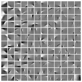
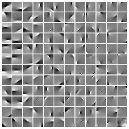
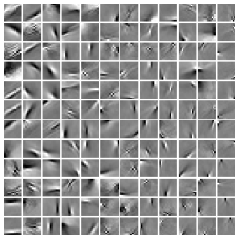
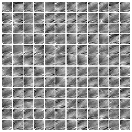
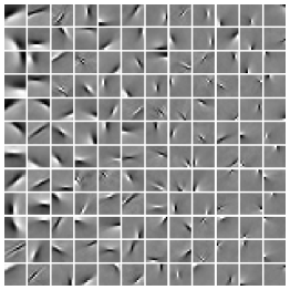
Figure 4: Comparison of basis vectors obtained by our method and other methods. Panel (a)–(e) correspond to panel (a)–(e) in Figure 2, where the basis vectors are given by (A.130). The basis vectors in panel (f) are learned by MBDL and given by (A.127).

A.5.2 Comparison of Basis Vectors

We compared our algorithm with an up-to-date sparse coding algorithm, the mini-batch dictionary learning (MBDL) as given in (Mairal et al.,, 2009; 2010) and integrated in Python library, i.e. scikit-learn. The input data was the same as the above, i.e. $10^{5}$ nature image patches preprocessed by the ZCA whitening filters.

We denotes the optimal dictionary learned by MBDL as $\mathbf{\check{B}}\in\mathbb{R}^{K\times K_{1}}$ for which each column represents a basis vector. Now we have

$$\mathbf{x} \approx\mathbf{{\mathbf{U}\boldsymbol{\Sigma}}}^{1/2}\mathbf{{\mathbf{U}}}^{T}\mathbf{\check{B}y}=\mathbf{\tilde{B}y}\text{,}$$ (A.126)

$$\mathbf{\tilde{B}} =\mathbf{{\mathbf{U}\boldsymbol{\Sigma}}}^{1/2}\mathbf{{\mathbf{U}}}^{T}\mathbf{\check{B}}\text{,}$$ (A.127)

where $\mathbf{y}=\left(y_{1},\cdots,y_{K_{1}}\right)^{T}$ is the coefficient vector.

Similarly, we can obtain a dictionary from the filter matrix $\mathbf{C}$. Suppose $\mathrm{rank}\left({\mathbf{C}}\right)={K_{0}}\leq K_{1}$, then it follows from (A.64) that

$$\mathbf{\hat{x}}=\left(a{\mathbf{CC}}^{T}\right)^{-1}{\mathbf{C}}\mathbf{y}\text{.}$$ (A.128)

By (A.66) and (A.128), we get

$$\mathbf{x} \approx\mathbf{By}=a\mathbf{B}{\mathbf{C}}^{T}\mathbf{{\boldsymbol{\Sigma}}}_{0}^{-1/2}\mathbf{{\mathbf{U}}}_{0}^{T}\mathbf{x}\text{,}$$ (A.129)

$$\mathbf{B} =a^{-1}\mathbf{{\mathbf{U}}}_{0}\mathbf{{\boldsymbol{\Sigma}}}_{0}^{1/2}\left({\mathbf{CC}}^{T}\right)^{-1}{\mathbf{C}}=\left[\mathbf{b}_{1},\cdots,\mathbf{b}_{K_{1}}\right]\text{,}$$ (A.130)

where $\mathbf{y}=\mathbf{W}^{T}\mathbf{x}=a{\mathbf{C}}^{T}\mathbf{{\boldsymbol{\Sigma}}}_{0}^{-1/2}\mathbf{{\mathbf{U}}}_{0}^{T}\mathbf{x}$, the vectors $\mathbf{b}_{1},\cdots,\mathbf{b}_{K_{1}}$ can be regarded as the basis vectors and the strict equality holds when $K_{0}=K_{1}=K$. Recall that $\mathbf{X}=[\mathbf{x}_{1}$, $\cdots$, $\mathbf{x}_{M}]=\mathbf{US\tilde{V}}^{T}$ (see Eq. A.49) and $\mathbf{Y}=[\mathbf{y}_{1}$,  $\cdots$, $\mathbf{y}_{M}]=\mathbf{W}^{T}\mathbf{X}=a\sqrt{M-1}{\mathbf{C}}^{T}\mathbf{\tilde{V}}_{0}^{T}$, then we get $\mathbf{\breve{X}}=\mathbf{BY}=\sqrt{M-1}\mathbf{{\mathbf{U}}}_{0}\mathbf{{\boldsymbol{\Sigma}}}_{0}^{1/2}\mathbf{\tilde{V}}_{0}^{T}\approx\mathbf{X}$. Hence, Eq. (A.129) holds.

The basis vectors shown in Figure 4–4 correspond to filters in Figure 2–2. And Figure 4 illustrates the optimal dictionary $\mathbf{\tilde{B}}$ learned by MBDL, where we set the regularization parameter as $\lambda=1.2/\sqrt{K}$, the batch size as $50$ and the total number of iterations to perform as $20000$, which took about $3$ hours for training. From Figure 4 we see that these basis vectors obtained by the above algorithms have local Gabor-like shapes except for those by SRBM. If $\mathrm{rank}(\mathbf{\check{B})}=K=K_{1}$, then the matrix $\mathbf{\check{B}}^{-T}$ can be regarded as a filter matrix like matrix ${\mathbf{\check{C}}}$ (see Eq. A.69). However, from the column vector of matrix $\mathbf{\check{B}}^{-T}$ we cannot find any local Gabor-like filter that resembles the filters shown in Figure 2. Our algorithm has less computational cost and a much faster convergence rate than the sparse coding algorithm. Moreover, the sparse coding method involves a dynamic generative model that requires relaxation and is therefore unsuitable for fast inference, whereas the feedforward framework of our model is easy for inference because it only requires evaluating the nonlinear tuning functions.

A.5.3 Learning Overcomplete Bases

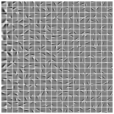
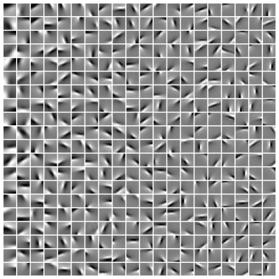
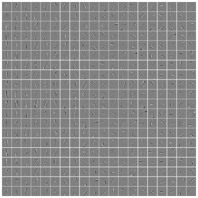
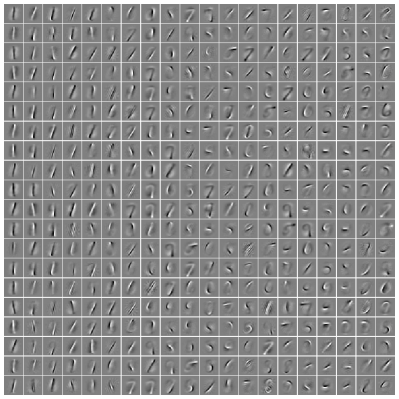
Figure 5: Filters and bases obtained from Olshausen’s image dataset and MNIST dataset by Algorithm 2. (a) and (b): $400$ typical filters and the corresponding bases obtained from Olshausen’s image dataset, where $K_{0}=82$ and $K_{1}=1024$. (c) and (d): $400$ typical filters and the corresponding bases obtained from the MNIST dataset, where $K_{0}=183$ and $K_{1}=1024$.

We have trained our model on the Olshausen’s nature image patches with a highly overcomplete setup by optimizing the objective (A.118) by Alg.2 and got Gabor-like filters. The results of $400$ typical filters chosen from $1024$ output filters are displayed in Figure 5 and corresponding base (see Eq. A.130) are shown in Figure 5. Here the parameters are $K_{1}=1024$, $t_{\max}=100$, ${v}_{1}=0.4$, $\tau=0.8$, and $\epsilon=0.98$ (see A.52), from which we got $\mathrm{rank}\left(\mathbf{B}\right)=K_{0}=82$. Compared to the ICA-like results in Figure 2–2, the average size of Gabor-like filters in Figure 5 is bigger, indicating that the small noise-like local structures in the images have been filtered out.

We have also trained our model on 60,000 images of handwritten digits from MNIST dataset (LeCun et al.,, 1998) and the resultant $400$ typical optimal filters and bases are shown in Figure 5 and Figure 5, respectively. All parameters were the same as Figure 5 and Figure 5: $K_{1}=1024$, $t_{\max}=100$, $v_{1}=0.4$, $\tau=0.8$ and $\epsilon=0.98$, from which we got $\mathrm{rank}\left(\mathbf{B}\right)=K_{0}=183$. From these figures we can see that the salient features of the input images are reflected in these filters and bases. We could also get the similar overcomplete filters and bases by SRBM and MBDL. However, the results depended sensitively on the choice of parameters and the training took a long time.

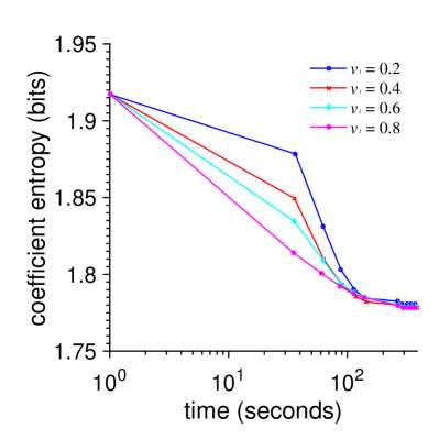
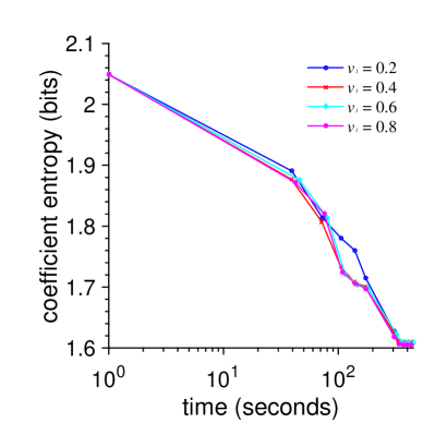
Figure 6: CFE as a function of training time for Alg.2, with ${v}_{1}=0.2$, $0.4$, $0.6$ or $0.8$. In all experiments parameters were set to $t_{\max}=100$, $t_{0}=50$ and $\tau=0.8$. (a): corresponding to Figure 5 or Figure 5. (b): corresponding to Figure 5 or Figure 5.

Figure 6 shows that CFE as a function of training time for Alg.2, where Figure 6 corresponds to Figure 5-5 for learning nature image patches and Figure 6 corresponds to Figure 5-5 for learning MNIST dataset. We set parameters $t_{\max}=100$ and $\tau=0.8$ for all experiments and varied parameter ${v}_{1}$ for each experiment, with ${v}_{1}=0.2$, $0.4$, $0.6$ or $0.8$. These results indicate a fast convergence rate for training on different datasets. Generally, the convergence is insensitive to the change of parameter ${v}_{1}$.

We have also performed additional tests on other image datasets and got similar results, confirming the speed and robustness of our learning method. Compared with other methods, e.g., IICA, FICA, MBDL, SRBM or sparse autoencoders etc., our method appeared to be more efficient and robust for unsupervised learning of representations. We also found that complete and overovercomplete filters and bases learned by our methods had local Gabor-like shapes while the results by SRBM or MBDL did not have this property.

A.5.4 Image Denoising

Similar to the sparse coding method applied to image denoising (Elad & Aharon,, 2006), our method (see Eq. A.130) can also be applied to image denoising, as shown by an example in Figure 7. The filters or bases were learned by using $7\times 7$ image patches sampled from the left half of the image, and subsequently used to reconstruct the right half of the image which was distorted by Gaussian noise. A common practice for evaluating the results of image denoising is by looking at the difference between the reconstruction and the original image. If the reconstruction is perfect the difference should look like Gaussian noise. In Figure 7 and 7 a dictionary ($100$ bases) was learned by MBDL and orthogonal matching pursuit was used to estimate the sparse solution. For our method (shown in Figure 7), we first get the optimal filters parameter $\mathbf{W}$, a low rank matrix ($K_{0}<K$), then from the distorted image patches $\mathbf{x}_{m}$ ($m=1,\cdots,M$) we get filter outputs $\mathbf{y}_{m}=\mathbf{W}^{T}\mathbf{x}_{m}$ and the reconstruction $\mathbf{\breve{x}}_{m}=\mathbf{By}_{m}$ (parameters: $\epsilon=0.975$ and $K_{0}=K_{1}=14$). As can be seen from Figure 7, our method worked better than dictionary learning, although we only used $14$ bases compared with $100$ bases used by dictionary learning. Our method is also more efficient. We can get better optimal bases $\mathbf{B}$ by a generative model using our infomax approach (details not shown).

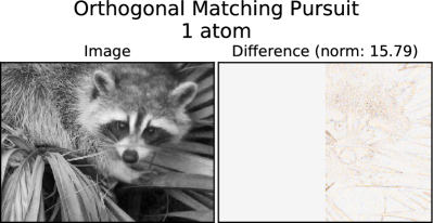
Figure 7: Image denoising. (a): the right half of the original image is distorted by Gaussian noise and the norm of the difference between the distorted image and the original image is $23.48$. (b): image denoising by our method (Algorithm 1), with $14$ bases used. (c) and (d): image denoising using dictionary learning, with $100$ bases used.

References

- Aharon et al., (2006) Aharon, M., Elad, M., & Bruckstein, A. (2006). K-SVD: An algorithm for designing overcomplete dictionaries for sparse representation. Signal Processing, IEEE Transactions on, 54(11), 4311–4322.
- Amari, (1999) Amari, S. (1999). Natural gradient learning for over- and under-complete bases in ica. Neural Comput., 11(8), 1875–1883.
- Atick, (1992) Atick, J. J. (1992). Could information theory provide an ecological theory of sensory processing? Network: Comp. Neural., 3(2), 213–251.
- Barlow, (1961) Barlow, H. B. (1961). Possible principles underlying the transformation of sensory messages. Sensory Communication, (pp. 217–234).
- Bell & Sejnowski, (1995) Bell, A. J. & Sejnowski, T. J. (1995). An information-maximization approach to blind separation and blind deconvolution. Neural Comput., 7(6), 1129–1159.
- Bell & Sejnowski, (1997) Bell, A. J. & Sejnowski, T. J. (1997). The ”independent components” of natural scenes are edge filters. Vision Res., 37(23), 3327–3338.
- Bengio, (2012) Bengio, Y. (2012). Deep learning of representations for unsupervised and transfer learning. Unsupervised and Transfer Learning Challenges in Machine Learning, 7, 19.
- Bengio et al., (2013) Bengio, Y., Courville, A., & Vincent, P. (2013). Representation learning: A review and new perspectives. Pattern Analysis and Machine Intelligence, IEEE Transactions on, 35(8), 1798–1828.
- Bengio et al., (2007) Bengio, Y., Lamblin, P., Popovici, D., Larochelle, H., et al. (2007). Greedy layer-wise training of deep networks. Advances in neural information processing systems, 19, 153.
- Borst & Theunissen, (1999) Borst, A. & Theunissen, F. E. (1999). Information theory and neural coding. Nature neuroscience, 2(11), 947–957.
- Carlo & Stevens, (2013) Carlo, C. N. & Stevens, C. F. (2013). Structural uniformity of neocortex, revisited. Proceedings of the National Academy of Sciences, 110(4), 1488–1493.
- Coates et al., (2011) Coates, A., Ng, A. Y., & Lee, H. (2011). An analysis of single-layer networks in unsupervised feature learning. In International conference on artificial intelligence and statistics (pp. 215–223).
- Cortes & Vapnik, (1995) Cortes, C. & Vapnik, V. (1995). Support-vector networks. Machine learning, 20(3), 273–297.
- Cover & Thomas, (2006) Cover, T. M. & Thomas, J. A. (2006). Elements of Information, 2nd Edition. New York: Wiley-Interscience.
- Edelman et al., (1998) Edelman, A., Arias, T. A., & Smith, S. T. (1998). The geometry of algorithms with orthogonality constraints. SIAM J. Matrix Anal. Appl., 20(2), 303–353.
- Elad & Aharon, (2006) Elad, M. & Aharon, M. (2006). Image denoising via sparse and redundant representations over learned dictionaries. Image Processing, IEEE Transactions on, 15(12), 3736–3745.
- Erhan et al., (2010) Erhan, D., Bengio, Y., Courville, A., Manzagol, P.-A., Vincent, P., & Bengio, S. (2010). Why does unsupervised pre-training help deep learning? The Journal of Machine Learning Research, 11, 625–660.
- Goodfellow et al., (2014) Goodfellow, I., Pouget-Abadie, J., Mirza, M., Xu, B., Warde-Farley, D., Ozair, S., Courville, A., & Bengio, Y. (2014). Generative adversarial nets. In Advances in Neural Information Processing Systems (pp. 2672–2680).
- Hinton, (2010) Hinton, G. (2010). A practical guide to training restricted boltzmann machines. Momentum, 9(1), 926.
- Hinton et al., (2006) Hinton, G., Osindero, S., & Teh, Y.-W. (2006). A fast learning algorithm for deep belief nets. Neural computation, 18(7), 1527–1554.
- Hinton & Salakhutdinov, (2006) Hinton, G. E. & Salakhutdinov, R. R. (2006). Reducing the dimensionality of data with neural networks. Science, 313(5786), 504–507.
- Huang & Zhang, (2016) Huang, W. & Zhang, K. (2016). Information-theoretic bounds and approximations in neural population coding. Neural Comput, submitted, URL https://arxiv.org/abs/1611.01414.
- Hubel & Wiesel, (1962) Hubel, D. H. & Wiesel, T. N. (1962). Receptive fields, binocular interaction and functional architecture in the cat’s visual cortex. The Journal of physiology, 160(1), 106–154.
- Hyvärinen, (1999) Hyvärinen, A. (1999). Fast and robust fixed-point algorithms for independent component analysis. Neural Networks, IEEE Transactions on, 10(3), 626–634.
- Karklin & Simoncelli, (2011) Karklin, Y. & Simoncelli, E. P. (2011). Efficient coding of natural images with a population of noisy linear-nonlinear neurons. In Advances in neural information processing systems, volume 24 (pp. 999–1007).
- Konstantinides & Yao, (1988) Konstantinides, K. & Yao, K. (1988). Statistical analysis of effective singular values in matrix rank determination. Acoustics, Speech and Signal Processing, IEEE Transactions on, 36(5), 757–763.
- Kreutz-Delgado et al., (2003) Kreutz-Delgado, K., Murray, J. F., Rao, B. D., Engan, K., Lee, T. S., & Sejnowski, T. J. (2003). Dictionary learning algorithms for sparse representation. Neural computation, 15(2), 349–396.
- LeCun et al., (1998) LeCun, Y., Bottou, L., Bengio, Y., & Haffner, P. (1998). Gradient-based learning applied to document recognition. Proceedings of the IEEE, 86(11), 2278–2324.
- Lee et al., (2006) Lee, H., Battle, A., Raina, R., & Ng, A. Y. (2006). Efficient sparse coding algorithms. In Advances in neural information processing systems (pp. 801–808).
- Lee et al., (2008) Lee, H., Ekanadham, C., & Ng, A. Y. (2008). Sparse deep belief net model for visual area v2. In Advances in neural information processing systems (pp. 873–880).
- Lewicki & Olshausen, (1999) Lewicki, M. S. & Olshausen, B. A. (1999). Probabilistic framework for the adaptation and comparison of image codes. JOSA A, 16(7), 1587–1601.
- Lewicki & Sejnowski, (2000) Lewicki, M. S. & Sejnowski, T. J. (2000). Learning overcomplete representations. Neural computation, 12(2), 337–365.
- Linsker, (1988) Linsker, R. (1988). Self-Organization in a perceptual network. Computer, 21(3), 105–117.
- Mairal et al., (2009) Mairal, J., Bach, F., Ponce, J., & Sapiro, G. (2009). Online dictionary learning for sparse coding. In Proceedings of the 26th annual international conference on machine learning (pp. 689–696).: ACM.
- Mairal et al., (2010) Mairal, J., Bach, F., Ponce, J., & Sapiro, G. (2010). Online learning for matrix factorization and sparse coding. The Journal of Machine Learning Research, 11, 19–60.
- Montufar et al., (2014) Montufar, G. F., Pascanu, R., Cho, K., & Bengio, Y. (2014). On the number of linear regions of deep neural networks. In Advances in Neural Information Processing Systems (pp. 2924–2932).
- Nair & Hinton, (2010) Nair, V. & Hinton, G. E. (2010). Rectified linear units improve restricted boltzmann machines. In Proceedings of the 27th International Conference on Machine Learning (ICML-10) (pp. 807–814).
- Olshausen & Field, (1996) Olshausen, B. A. & Field, D. J. (1996). Emergence of simple-cell receptive field properties by learning a sparse code for natural images. Nature, 381(6583), 607–609.
- Olshausen & Field, (1997) Olshausen, B. A. & Field, D. J. (1997). Sparse coding with an overcomplete basis set: A strategy employed by v1? Vision Res., 37(23), 3311–3325.
- Rao, (1945) Rao, C. R. (1945). Information and accuracy attainable in the estimation of statistical parameters. Bulletin of the Calcutta Mathematical Society, 37(3), 81–91.
- Shannon, (1948) Shannon, C. (1948). A mathematical theory of communications. Bell System Technical Journal, 27, 379–423 and 623–656.
- Srivastava et al., (2014) Srivastava, N., Hinton, G., Krizhevsky, A., Sutskever, I., & Salakhutdinov, R. (2014). Dropout: A simple way to prevent neural networks from overfitting. The Journal of Machine Learning Research, 15(1), 1929–1958.
- Vincent et al., (2010) Vincent, P., Larochelle, H., Lajoie, I., Bengio, Y., & Manzagol, P.-A. (2010). Stacked denoising autoencoders: Learning useful representations in a deep network with a local denoising criterion. The Journal of Machine Learning Research, 11, 3371–3408.
- Yarrow et al., (2012) Yarrow, S., Challis, E., & Series, P. (2012). Fisher and shannon information in finite neural populations. Neural computation, 24(7), 1740–1780.