Photoelectron angular distribution in two-pathway ionization of neon with femtosecond XUV pulses

Abstract

We analyze the photoelectron angular distribution in two-pathway interference between nonresonant one-photon and resonant two-photon ionization of neon. We consider a bichromatic femtosecond XUV pulse whose fundamental frequency is tuned near the $2p^{5}3s$ atomic states of neon. The time-dependent Schrödinger equation is solved and the results are employed to compute the angular distribution and the associated anisotropy parameters at the main photoelectron line. We also employ a time-dependent perturbative approach, which allows obtaining information on the process for a large range of pulse parameters, including the steady-state case of continuous radiation, i.e., an infinitely long pulse. The results from the two methods are in relatively good agreement over the domain of applicability of perturbation theory.

I Introduction

Recent improvements in advanced light sources have opened up a variety of new promising possibilities regarding the coherent control of atomic systems in the extreme ultraviolet (XUV) energy range. One way to achieve coherent control of the photoelectron angular distribution (PAD), which has been experimentally realized with atoms 25 years ago by optical lasers, is to interfere one-photon and two-photon ionization pathways Baranova92 ; Yin92 . The two-photon and one-photon pathways are, respectively, produced by the fundamental and the second harmonic of the optical laser. We will refer to this particular case as an $\omega+2\,\omega$ process below. This field originated in theory and was further developed experimentally Baranova91 ; Schafer92 ; Wang01 ; Yamazaki07 . Coherent control via two-pathway interference was reviewed, for instance, in Ehlotzky01 ; Astapenko06 .

In certain cases, resonant ionization via an intermediate state can be used to enhance the two-photon pathway Yin95 ; Grum15 ; Prince16 ; Douguet16 . The coherent XUV pulses from the Free-Electron Laser (FEL) at FERMI (Trieste, Italy) recently allowed for the experimental manipulation of the PAD by controlling the relative time-delay between the fundamental and the second harmonic of a linearly polarized XUV femtosecond (fs) pulse to an unprecedented time resolution of 3.1 attoseconds (as) Prince16 . The experimental study employed neon as the atomic target, with one of the $(2p^{5}4s)$ states with total electronic angular momentum $J=1$ as an intermediate stepping stone, by utilizing a two-color pulse of central wavelengths 63.0 and 31.5 nm, respectively.

In light of the experimental success and further expected investigations regarding coherent control of the PAD in neon, it is highly desirable that such complex and expensive experiments are supported by theoretical efforts. Therefore, one of the principal goals of the present work is to reveal some of the main characteristics of the $\omega+2\,\omega$ process in neon, this time choosing $(2p^{5}3s)\,J=1$ as the intermediate states. We picked the latter states for the present study, since they can be reasonably well described in a nonrelativistic $LS$-coupling scheme, while the two $(2p^{5}4s)\,J=1$ states require an intermediate coupling description due to the lack of a well-defined total spin.

In the theoretical work described below, we employed three different methods to describe the $\omega+2\,\omega$ process. In the first one, we solved the time-dependent Schrödinger equation (TDSE) numerically on a grid Grum06 , using a single-active electron (SAE) potential to accurately represent the energies and one-electron orbitals of neon. In the second method, we employed a time-dependent lowest (nonvanishing) order perturbation theory (PT) approach with the target structure obtained from a multi-configuration Hartree-Fock (MCHF) calculation and only a few intermediate states accounted for in the second-order PT ionization amplitude. Finally, we considered pulses with an infinite number of cycles (PT-$\infty$) using a variationally stable method Gao88 ; Orel88 ; Gao90 ; Staroselskaya15 , which effectively accounts for all intermediate states in the second-order PT ionization amplitude.

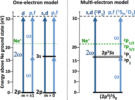
Figure 1: $\omega+2\,\omega$ ionization scheme by linearly polarized light in neon with $(2p^{5}3s)\rm^{1}P$ as the intermediate state in the single-active-electron model (left) and both $(2p^{5}3s)\;J=1$ states in the multi-electron model (right). See text for details.

There exist two states, $2p^{5}{\rm(^{2}P_{3/2})}3s$ and $2p^{5}{\rm(^{2}P_{1/2})}3s$, with total angular momentum $J=1$, which can be reached via optically allowed transitions from the $(2p^{6})\rm^{1}S_{0}$ initial state. As previously mentioned, these states are relatively well described in the $LS$-coupling scheme, since they have predominant (93$\%$ Machado ; NIST ) $\rm{}^{3}P$ and $\rm{}^{1}P$ character, respectively. Therefore, we employ the $LS$-coupling scheme notations to label these states in the following development.

The $\omega+2\,\omega$ process using $(2p^{5}3s)\,J=1$ as intermediate states is presented in Fig. 1. The scheme in the one-electron model is shown on the left panel, where we denote the electronic states by listing only the active electron. Therefore, the intermediate state (only the $\rm{}^{1}P$ state is possible) is simply labelled $3s$, and this notation will be further used throughout the manuscript. One-photon absorption of the second harmonic produces $s$- and $d$-wave photoelectrons, while two-photon absorption of the fundamental produces $p$- and $f$-wave photoelectrons. In the multi-electron model (right panel of Fig. 1), these waves couple to the residual ionic state to make the symmetries indicated at the top. The intermediate $\rm{}^{3}P_{1}$ and $\rm{}^{1}P_{1}$ states, corresponding to the $2p\to 3s$ one-electron excitation, have, respectively, 16.67 eV and 16.85 eV excitation energies NIST . Since only $\rm{}^{1}P_{1}$ can be efficiently excited, and it is well separated from other optically allowed states, it enables us to treat the effect of an “almost” isolated resonance. Consequently, it represents an excellent situation, with a minimum of additional complications, to compare results obtained by different models in a multi-electron system.

This manuscript is organized as follows. In the next section, we introduce our theoretical models, while Sect. III is devoted to the presentation and analysis of our results. Finally, Sect. IV contains our conclusions and perspectives for the future. Unless indicated otherwise, atomic units are used throughout this manuscript.

II Theoretical approach

We consider a linearly polarized electric field of the form

$$E(t)=F(t)\left[\cos\omega t+\eta\cos(2\,\omega t+\phi)\right]\,,$$ (1)

where $\eta$ represents the amplitude ratio between the harmonics, $\phi$ is the carrier envelope phase (CEP) of the second harmonic, and $F(t)$ is the envelope function. We employ the commonly used sine-squared envelope $F(t)=F_{0}\sin^{2}(\Omega t)$, where $\Omega=\omega/2N$, with $N\gg 1$ denoting the number of optical cycles.

The details of our TDSE approach can be found in Grum15 ; Grum06 ; Abeln2010 . The present TDSE calculations differ from our previous ones for electrons initially in an $s$-orbital in that we now independently propagate the electronic wave packets initially in the $2p\;(m=0,\pm 1)$ orbitals and then average the results over the magnetic quantum numbers $m$ to simulate an isotropic initial $2p^{6}\,\rm(^{1}S)$ state. Here we only show briefly the main steps in the PT approach and describe the physical models.

In second-order PT, the PAD for an initially unpolarized atom is given by

$$\frac{dW}{d\Omega}=\frac{C}{2J_{0}+1}\sum_{M_{0}\mu\atop{J_{f}M_{f}}}\left|\eta\,U^{(1)}_{J_{0}M_{0};J_{f}M_{f},\vec{k}\mu}+U^{(2)}_{J_{0}M_{0};J_{f}M_{f},\vec{k}\mu}\right|^{2},$$ (2)

where $\vec{k}$ is the linear momentum and $\mu$ the spin component of the photoelectron, respectively; $J_{0}$ is the initial total electronic angular momentum with projection $M_{0}$; $M_{f}$ is the projection of the residual ionic angular momentum $J_{f}$; $C$ is a normalization coefficient that is independent of the transition matrix elements and not relevant for our further derivations. In Eq. (2) we summed over $J_{f}$, assuming incoherently excited fine-structure levels of the residual ion.

We choose the quantization $z$-axis along the electric field of the laser beams. In the dipole approximation, the ionization amplitudes are given by

$$U^{(1)}_{J_{0}M_{0};J_{f}M_{f},\vec{k}\mu} = -i\mbox{$\langle J_{f}M_{f},\vec{k}\mu^{(-)}\,|\,D_{z}\,|\,J_{0}M_{0}\rangle$}\,T^{(1)},$$ (3)

$$U^{(2)}_{J_{0}M_{0};J_{f}M_{f},\vec{k}\mu} = -\int\hskip-15.649pt\sum_{~{}~{}n}\mbox{$\langle J_{f}M_{f},\vec{k}\mu^{(-)}\,|\,D_{z}\,|\,\zeta_{n}J_{n}M_{n}\rangle$}$$ (4)

$$~{}~{}\times\mbox{$\langle\zeta_{n}J_{n}M_{n}\,|\,D_{z}\,|\,J_{0}M_{0}\rangle$}\,T^{(2)}_{E_{n}}\,.$$

Here $D_{z}=\sum_{i}d_{z,i}=\sum_{i}z_{i}$ is the $z$-component of the dipole operator, where the summation is taken over all atomic electrons, and the sum (integral) in (4) is taken over all atomic states with bound (continuum) energy $E_{n}$, labeled with their angular momentum $J_{n}$, projection $M_{n}$, and the set of additional quantum numbers $\zeta_{n}$. The values of the time integrals $T^{(1)}$ and $T^{(2)}_{E_{n}}$ were given in Eqs. (9) and (10) of Ref. Grum15 (with the replacement $E_{1s}\to E_{2p}$). The superscript $(-)$ indicates the necessary asymptotic form of the continuum wave function, which is a distorted Coulomb wave calculated in the Hartree potential of the residual ion.

Upon expanding the ejected electron wave function $\mbox{$|\,\vec{k}\mu\,\rangle$}^{(-)}$ in Eqs. (3) and (4) in (nonrelativistic) partial waves and using standard angular momentum algebra, the PAD (2) may be written in the well-known form with Legendre polynomials $P_{k}(x)$ as

$$W(\theta)=\frac{W_{0}}{4\pi}\left(1+\sum_{k}\beta_{k}P_{k}(\cos\theta)\right)\,,$$ (5)

with $W_{0}$ the angle-integrated cross section. The anisotropy parameters $\beta_{k}$ are generally given by cumbersome expressions, including three types of terms, originating from the first-order amplitude (3), the second-order amplitude (4), and their interference.

In this paper, we are also interested in the differential asymmetry defined by Grum15

$$A(0)=\frac{W(0)-W(\pi)}{W(0)+W(\pi)}=\frac{\sum_{k=1,3,...}\beta_{k}}{1+\sum_{k=2,4,...}\beta_{k}}\,.$$ (6)

As seen from the last part of the equation, a nonzero asymmetry requires at least one nonvanishing odd-rank anisotropy parameter.

In the nonstationary PT version, we included seven intermediate excited states of Ne in the sum over $n$ in Eq. (4), all with total angular momentum $J_{n}=1$: two states with configuration $2p^{5}3s$, two states with $2p^{5}4s$, and three states with $2p^{5}3d$. The final ionic states Ne${}^{+}(2p^{5})^{2}{\rm P}_{1/2,3/2}$ were treated in the single-configuration Hartree-Fock approximation in the $LSJ$-coupling scheme. The wave functions of the photoelectron $\varepsilon\ell$ with energy $\varepsilon$ and orbital angular momentum $\ell$ were calculated in the Hartree-Fock frozen-core approximation Froese97 . For the states $|\,\zeta_{n}J_{n}=1\,\rangle$, we used the intermediate-coupling scheme and mixed the $2p^{5}3s$, $2p^{5}4s$, and $2p^{5}3d$ configurations on the basis of the term-averaged atomic electron orbitals. For the PADs in a narrow range of photon energies around the excitation energy of the $2p^{5}3s\,^{1}{\rm P}_{1}$ state, the effects of other $|\,\zeta_{n}J_{n}=1\,\rangle$ states, although being included, are not expected to be very important, due to negligible admixtures of other configurations and the weak violation of the $LS$-coupling.

More compact expressions can be obtained for the $\beta_{k}$ parameters in the single-configuration approximation and a pure $LS$-coupling scheme. After transforming from multi-electron matrix elements to single-electron matrix elements Sobelman72 ; Varshalovich88 , we obtain for ionization from the closed $2p^{6}$ shell of neon:

$$\beta_{k}=\beta^{(1)}_{k}+\beta^{(2)}_{k}+\beta^{(12)}_{k}\,,\qquad k=1,\,2,\,3,\,4.$$ (7)

The first term originates from the absolute square of the first-order amplitude and contributes only for $k=2$:

$$\beta^{(1)}_{k} = \frac{1}{N}\left|T^{(1)}\right|^{2}\sum_{\ell\ell^{\prime}m}\mbox{$(-1)^{m}$}\hat{\ell}\hat{\ell}^{\prime}\mbox{$\left(\ell 0,\ell^{\prime}0\,|\,k0\right)$}$$ (8)

$$\times\mbox{$\left(\ell m,\ell^{\prime}-m\,|\,k0\right)$}\mbox{$\left(1m,\ell-m\,|\,10\right)$}\mbox{$\left(1m,\ell^{\prime}-m\,|\,10\right)$}$$

$$\times e^{i(\Delta_{\ell}^{(1)}-\Delta_{\ell^{\prime}}^{(1)})}d_{\varepsilon\ell,2p}\,d_{\varepsilon\ell^{\prime},2p}^{\ast}\,.$$

In accordance with the selection rules for angular momentum and parity, the summation in (8) runs over $\ell=0,\,2$ and $\ell^{\prime}=0,\,2$ (at least one of $\ell$ or $\ell^{\prime}$ should be nonzero). The second term in (7) originates from the absolute square of the second-order amplitude and contributes for $k=2,\,4$:

$$\beta^{(2)}_{k} = \frac{\eta^{2}}{3N}\sum_{\ell\ell^{\prime}m}\mbox{$(-1)^{m}$}\hat{\ell}\hat{\ell}^{\prime}\mbox{$\left(\ell 0,\ell^{\prime}0\,|\,k0\right)$}\mbox{$\left(\ell m,\ell^{\prime}-m\,|\,k0\right)$}$$ (9)

$$\times e^{i(\Delta_{\ell}^{(2)}-\Delta_{\ell^{\prime}}^{(2)})}$$

$$\times\;\int\hskip-21.33955pt\sum_{~{}~{}~{}n,\ell_{n}}\mbox{$\left(\ell_{n}m,\ell-m\,|\,10\right)$}\mbox{$\left(1m,\ell_{n}-m\,|\,10\right)$}$$

$$~{}~{}~{}~{}~{}~{}~{}~{}~{}~{}~{}~{}~{}~{}~{}~{}~{}~{}~{}~{}\times T_{E_{n}}^{(2)}\,d_{\varepsilon\ell,nl_{n}}\,d_{n\ell_{n},2p}$$

$$\times\;\int\hskip-21.33955pt\sum_{~{}~{}~{}n^{\prime}\!,\ell^{\prime}_{n}}\mbox{$\left(\ell^{\prime}_{n}m,\ell^{\prime}-m\,|\,10\right)$}\mbox{$\left(1m,\ell^{\prime}_{n}-m\,|\,10\right)$}$$

$$~{}~{}~{}~{}~{}~{}~{}~{}~{}~{}~{}~{}~{}~{}~{}~{}~{}~{}~{}~{}\times T_{E_{n^{\prime}}}^{(2)\ast}\,d_{\varepsilon\ell^{\prime},n^{\prime}\ell^{\prime}_{n}}^{\ast}\,d_{n^{\prime}\ell_{n^{\prime}},2p}^{\ast}\,.$$

Here $\ell_{n}\!=\!0,\,2$; $\ell\!=\!1,\,3$; $\ell^{\prime}\!=\!1,\,3$. The third term in (7) represents the interference between the two amplitudes and contributes for $k\!=\!1,\,3$:

$$\beta^{(12)}_{k} = -\frac{2\eta}{\sqrt{3}N}{\rm Re}\Big{[}\sum_{\ell\ell^{\prime}m}\hat{\ell}\hat{\ell}^{\prime}\mbox{$\left(\ell 0,\ell^{\prime}0\,|\,k0\right)$}\mbox{$\left(\ell m,\ell^{\prime}-m\,|\,k0\right)$}$$ (10)

$$\times e^{i(\Delta_{\ell}^{(1)}-\Delta_{\ell^{\prime}}^{(2)})}\mbox{$\left(1m,\ell-m\,|\,10\right)$}T^{(1)}d_{\varepsilon\ell,2p}$$

$$\times\;\int\hskip-21.33955pt\sum_{~{}~{}~{}n,\ell_{n}}\mbox{$(-1)^{\ell_{n}}$}\mbox{$\left(\ell_{n}m,\ell^{\prime}-m\,|\,10\right)$}\mbox{$\left(1m,\ell_{n}-m\,|\,10\right)$}$$

$$~{}~{}~{}~{}~{}~{}~{}~{}~{}~{}~{}~{}~{}~{}~{}~{}~{}~{}~{}~{}\times T_{E_{n}}^{(2)\ast}\,d_{\varepsilon\ell^{\prime},n\ell_{n}}^{\ast}\,d_{n\ell_{n},2p}\Big{]}\,,$$

with $\ell_{n}\!=\!0,\,2$; $\ell^{\prime}_{n}\!=\!0,\,2$; $\ell\!=\!1,\,3$; $\ell^{\prime}=1,\,3$. Recall that nonvanishing odd-rank anisotropy parameters such as $\beta_{1}$ and $\beta_{3}$ are responsible for a nonzero left-right asymmetry (6). Thus, nonvanishing values of the asymmetry are due to interference between one-photon and two-photon ionization amplitudes.

In Eqs. (8)-(10)

$$N = \left|T^{(1)}\right|^{2}\sum_{\ell}\left|d_{\varepsilon\ell,2p}\right|^{2}$$ (11)

$$+\,\eta^{2}\sum_{\ell m}\Big{|}\,\,\int\hskip-18.49428pt\sum_{~{}~{}n,\ell_{n}}\mbox{$(-1)^{\ell_{n}}$}\hat{\ell}^{-1}_{n}\mbox{$\left(\ell_{n}m,\ell-m\,|\,10\right)$}$$

$$~{}~{}~{}~{}\times\mbox{$\left(1m,10\,|\,\ell_{n}m\right)$}\,T_{E_{n}}^{(2)}\,d_{\varepsilon\ell,nl_{n}}\,d_{n\ell_{n},2p}\Big{|}^{2}\,.$$

Furthermore, ${\rm Re}[X]$ in Eq. (10) denotes the real part of the complex quantity $X$, $\left(j_{1}m_{1},j_{2}m_{2}\,|\,j_{3}m_{3}\right)$ is a Clebsch-Gordan coefficient, and $\hat{a}\equiv\sqrt{2a+1}$. For convenience we separated the factor $i^{\ell}e^{i\delta_{\ell}}$ in the continuum wave function ($\delta_{\ell}$ is the scattering phase) from the single-electron reduced dipole matrix elements $d_{\varepsilon\ell,2p}=\mbox{$\langle\varepsilon\ell\,||\,d\,||\,2p\rangle$}$, $d_{\varepsilon\ell,nl_{n}}=\mbox{$\langle\varepsilon\ell\,||\,d\,||\,nl_{n}\rangle$}$, $d_{n\ell_{n},2p}=\mbox{$\langle n\ell_{n}\,||\,d\,||\,2p\rangle$}$, and we introduced the abbreviations $e^{i\Delta_{\ell}^{(1)}}\equiv i^{-\ell-1}e^{i\delta_{\ell}}$ and $e^{i\Delta_{\ell}^{(2)}}\equiv-i^{-\ell}e^{i\delta_{\ell}}$. For clarity, we left the summations over the projections $m$ in Eqs. (8)-(11) rather than working them out further and expressing the final results in terms of $nj$-symbols.

Equations (7)-(11) represent the SAE model within the PT for the finite pulse duration. To turn to the limit of the infinite pulse duration ($N\to\infty$, PT-$\infty$ model), the time factors $T^{(1)}$ and $T^{(2)}_{E_{n}}$ transform as Grum15

$$T^{(1)} \to \phantom{-}\frac{\sqrt{3}F_{0}}{4\sqrt{2}}\,e^{-i\phi}\,,$$ (12)

$$T^{(2)}_{E_{n}} \to -\frac{3F^{2}_{0}}{32}\,\frac{i}{E_{n}-E_{2p}-\omega+i0}.$$ (13)

These equations differ from Eqs. (18) and (19) of Grum15 by an additional phase factor incorporated into the definition of $\Delta$ and a factor $\sqrt{3/8}$ that accounts for changing the total intensity from a finite $\sin^{2}$ pulse to a constant one of infinite length.

In the variationally stable method, which is applicable to an infinite pulse duration, a variational procedure to find the extremum of a functional is used instead of summing (integrating) over the infinite set of intermediate states $n$ in Eqs. (9)-(11) after substituting (13). The method is described in detail in Staroselskaya15 ; Gao89 . Varying the functional we expanded, following Gao88 ; Gao90 ; Staroselskaya15 and others, the trial radial functions $\lambda(r)$ and $\mu(r)$ over the basis of Slater orbitals $\Phi_{q}(r)=N_{q}r^{\ell_{n}+q}e^{-\chi r}$ as

$$\lambda(r)=\sum_{q=1}^{Q}a_{q}\Phi_{q}(r)\,,\quad\mu(r)=\sum_{q=1}^{Q}b_{q}\Phi_{q}(r)\,.$$ (14)

Here $Q$ is the number of Slater s orbitals, $N_{q}$ are normalization factors, the coefficients $a_{q}$ and $b_{q}$ are the parameters to be varied, and $\chi$ is a constant whose value is taken to improve convergence. In our case $Q=50$ and $\chi=2.5$. We used the electron wave functions of the initial and final states found in the Hartree-Fock-Slater Herman63 local potential. The latter is also taken as the radial part of the atomic Hamiltonian when calculating the functional.

Qualitatively, the behavior of the asymmetry parameters $\beta_{k}$ in the region of the $3s$ state can be understood within a simplified PT approach, which includes only a single intermediate $3s$ state. Using Eqs. (7)-(13), the anisotropy parameters $\beta_{k}$ may be reduced, for an infinite pulse, to simple parametric forms. Similar formulas were derived in Grum15 for $\omega+2\,\omega$ ionization of an $s$-electron in the vicinity of an isolated intermediate state, where the active electron occupies a $p$-orbital. Specifically:

$$\beta_{1} = \frac{\epsilon}{\epsilon^{2}+1}B_{1}\cos(\phi+\phi_{1})\,,$$ (15)

$$\beta_{2} = B_{2}\frac{\epsilon^{2}}{\epsilon^{2}+1}+\frac{2}{\epsilon^{2}+1}\,,$$ (16)

$$\beta_{3} = \frac{\epsilon}{\epsilon^{2}+1}B_{3}\cos(\phi+\phi_{3})\,,$$ (17)

$$\epsilon = \frac{\Delta\omega}{\frac{1}{2}\Gamma_{\beta}}\,,\quad\Delta\omega=\omega-(E_{3s}-E_{2p})\,,$$ (18)

$$\Gamma_{\beta} = \frac{F_{0}|d_{\epsilon p,3s}d_{3s,2p}|}{2\eta\sqrt{2(|d_{\epsilon s,2p}|^{2}+|d_{\epsilon d,2p}|^{2})}}\,,$$ (19)

$$B_{1} = \frac{\sqrt{3}|(2e^{i\Delta_{s}^{(1)}}d_{\epsilon s,2p}-\frac{4\sqrt{2}}{5}e^{i\Delta_{d}^{(1)}}d_{\epsilon d,2p})|}{\sqrt{|d_{\epsilon s,2p}|^{2}+|d_{\epsilon d,2p}|^{2}}}\,,$$ (20)

$$B_{2} = \frac{|d_{\epsilon d,2p}|^{2}-2\sqrt{2}\Re[e^{i(\Delta_{s}^{(1)}-\Delta_{d}^{(1)})}d_{\epsilon s,2p}d_{\epsilon d,2p}]}{|d_{\epsilon s,2p}|^{2}+|d_{\epsilon d,2p}|^{2}}\,,$$ (21)

$$B_{3} = \frac{6\sqrt{6}|d_{\epsilon d,2p}|}{5\sqrt{|d_{\epsilon s,2p}|^{2}+|d_{\epsilon d,2p}|^{2}}}\,,$$ (22)

$$\phi_{1} = \arg\Bigg{[}\left(2e^{i\Delta_{s}^{(1)}}d_{\epsilon s,2p}-\frac{4\sqrt{2}}{5}e^{i\Delta_{d}^{(1)}}d_{\epsilon d,2p}\right)$$ (23)

$$~{}~{}~{}~{}~{}~{}~{}~{}~{}\times e^{-i\Delta_{p}^{(2)}}d_{\epsilon p,3s}d_{3s,2p}\Bigg{]}\,,$$

$$\phi_{3} = \arg\left[-e^{i(\Delta_{d}^{(1)}-\Delta_{p}^{(2)})}d_{\epsilon d,2p}d_{\epsilon p,3s}d_{3s,2p}\right]\,.$$ (24)

In the above simplified PT approach, $\beta_{4}$, as well as all higher-rank anisotropy parameters, vanish. It is somewhat surprising that the parameters $B_{1},\,B_{2},\,B_{3}$ depend neither on the two-photon amplitude nor on $\eta$ in this simplified case. For infinite pulse duration within perturbation theory, therefore, the maximum asymmetry and phase do not depend on the strength of the second harmonic. However, the strength of the second harmonic affects the width of the asymmetry structure. The above features will be clearly seen below in the results of particular PT-$\infty$ calculations.

III Results and discussion

The numerical calculations were performed for two sets of pulse parameters. In the first set, we used a pulse $\Pi_{1}$, with $N=250$ cycles and the second-harmonic intensity set to $1\%$ of the fundamental intensity, i.e., $\eta=0.1$. In the second set, we used a longer pulse $\Pi_{2}$, with $N=500$ cycles and a higher intensity ratio of the second harmonic equal to 10$\%$ of the fundamental, i.e., $\eta=\sqrt{0.1}$ In both cases, the peak intensity of the fundamental was kept constant at 10¹²W/cm².

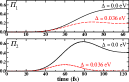
Figure 2: TDSE predictions for the population of the $3s$ state as a function of time. Results are shown for two different sets of pulse parameters. The fundamental frequency $\omega$ is either in resonance with the $3s$ intermediate state ($\Delta=0.0$ eV), or slightly detuned ($\Delta=0.036$ eV).

It is instructive to first analyze the efficiency of the femtosecond pulses in pumping the neon ground state to the excited $3s$ state. Figure 2 shows the evolution of the $3s$ state population as a function of time, for both $\Pi_{1}$ and $\Pi_{2}$, and for two different detunings $\Delta$ of the fundamental frequency.

The results behave in a predictable way. Focusing first on the resonant case ($\Delta=0.0$ eV), it is seen that the system does not even carry out half a Rabi oscillation for $\Pi_{1}$, whereas, for the longer pulse $\Pi_{2}$, the system is close to have undergone one complete such oscillation. In both cases the $3s$ population can reach large values, representing at their maximum, respectively, $51\%$ and $66\%$ of the total probability for $\Pi_{1}$ and $\Pi_{2}$. Note, however, that a significant occupation of the $3s$ state occurs on rather different time scales for both pulses. For example, the population of the $3s$ state is larger than $0.2$ for only $30$ fs during the pulse $\Pi_{1}$, but for more than $70$ fs during $\Pi_{2}$. In the detuned case ($\Delta=0.036$ eV), the $3s$ population decreases by slightly more than half for $\Pi_{1}$ in comparison with the resonant case, whereas the population is drastically diminished for $\Pi_{2}$. This characteristic is readily understood: Since the spectral spread of $\Pi_{2}$ is about half that of $\Pi_{1}$, the potential to drive an efficient population transfer decreases faster with increased detuning for $\Pi_{2}$ than for $\Pi_{1}$.

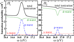
Figure 3: TDSE results for ionization to partial $s$-, $p$-, and $d$-waves, as well as total ionization at the main photoelectron line, for the $\Pi_{1}$ and $\Pi_{2}$ pulses.

Turning now to the analysis of the ionization process, we present in Fig. 3 the partial-wave contributions for $s$-, $p$-, and $d$-waves, and the total ionization probability, at the main photoelectron line, for both pulses. Out of resonance, both pulses exhibit similar characteristics, although ionization is of course much more likely for the $\Pi_{2}$ since (i) it is a longer pulse and (ii) the strength of the second harmonic is ten times larger than for $\Pi_{1}$. In addition, the ionization out of resonance is strongly dominated by the $d$-wave, representing more than $90\%$ of the total ionization probability in both cases.

On the other hand, one clearly observes two drastically different situations near resonance for each pulse. In the first case ($\Pi_{1}$), while the second harmonic is weak at the resonance, the resonant $p$-wave ionization represents a large part of the (small) total ionization probability. Note that the $p$-wave and $d$-wave contributions are nearly equal at resonance. Consequently, a strong peak appears in the ionization spectrum when the fundamental frequency spans the resonance. In the second case ($\Pi_{2}$), the second harmonic is so strong that the background $d$-wave ionization strongly dominates the resonant $p$-wave ionization. Since both $d$-wave and $s$-wave partial-wave ionization probabilities also decrease significantly at the resonance, the total ionization probability barely reveals a fingerprint of the resonance, apart from a small quenching. The dip in the partial $s$-wave and $d$-wave ionization probabilities for $\Pi_{2}$ at resonance is readily explained by the fact that the $2p$ orbital is strongly depleted over time by efficient pumping from $2p$ to $3s$ via the fundamental frequency.

The calculated TDSE and PT values of the anisotropy parameters, introduced in Eq. (5), are presented in Fig. 4 for ionization via $\Pi_{1}$. We only show $\beta_{k}$ for $k\leq 4$, since for the comparatively weak fields considered here, i.e., in the multi-photon regime, they represent the only significant nonvanishing elements. We observe an overall satisfactory agreement between the TDSE and PT results. The odd-rank anisotropy parameters, presented for both cases of $\phi=0$ and $\phi=\pi/2$, exhibit an asymmetric Fano-like profile near resonance. Even far from resonance, $\beta_{1}$ and $\beta_{3}$ assume nonnegligible values due to the spectral spread of $\Pi_{1}$. The anisotropy parameter $\beta_{2}$ peaks at resonance according to the increase in $p$-wave ionization (see Eq. (16)), while $\beta_{4}$ becomes negligible everywhere. Note that the finite pulse duration leads not only to the broadening of the profile of the $\beta_{1}$ and $\beta_{3}$ parameters, but also to an energy shift of their zero crossing (see Eqs. (15) and (17)) from the resonance position.

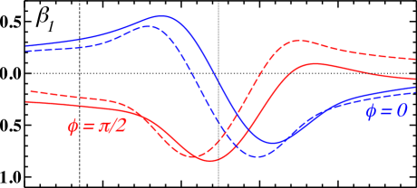
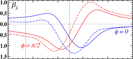
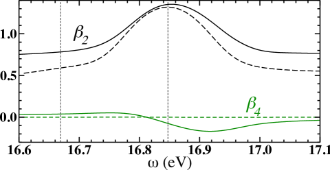
Figure 4: Anisotropy parameters $\beta_{1}$, $\beta_{2}$, $\beta_{3}$, and $\beta_{4}$, as a function of the fundamental frequency, for the pulse $\Pi_{1}$. Results are presented from both the TDSE (solid lines) and PT (dashed lines) approaches, and for CEPs $\phi=0$ and $\phi=\pi/2$ for $\beta_{1}$ and $\beta_{3}$. The left and right vertical lines indicate the energy positions of the two $2p^{5}3s$ states with $J=1$ and predominant triplet and singlet character, respectively.

There are two principal reasons for the small discrepancies between the TDSE and PT results. To begin with, they can be attributed to the different electronic structure models in each approach. Recall that the PT model uses a multi-electron MCHF description, while the solutions of the TDSE are obtained from a SAE potential. On the other hand, it was shown that the population of the $3s$ state can reach nonnegligible values, thus questioning the applicability of the PT approach. Despite these differences, the overall satisfactory agreement obtained between the results from these two treatments suggests that the principal physics of the $\omega+2\,\omega$ process is properly accounted for in both approaches.

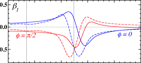
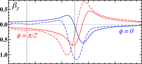
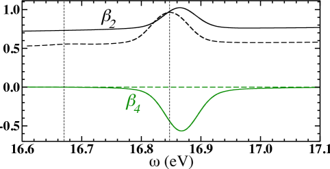
Figure 5: Same as Fig. 4 for the pulse $\Pi_{2}$.

The calculated anisotropy parameters associated with ionization by the pulse $\Pi_{2}$ are presented in Fig. 5. Since the pulse is longer, the width of the resonance profile is significantly narrower. As a result, the anisotropy parameters vary less and assume small values as the fundamental frequency is detuned from resonance. The small effect of the other $3s$ state at $16.67$ eV can actually be noticed in the PT results. Recall that this state is not included in the TDSE calculations. The values of $\beta_{1}$ and $\beta_{3}$ from TDSE and PT agree well for detunings $\Delta\geq 0.1$ eV. On the other hand, far from resonance, the $\beta_{2}$’s calculated in each approach exhibit a small discrepancy from each other, presumably due to the different structure models employed. Here one can directly compare with experimental data to assess the validity of the results. At $\omega=16.6$ eV, i.e., at $11.6$ eV photoelectron energy, the values of $\beta_{2}$, which are barely affected by resonance effects, are $0.72$, $0.53$, and $0.60$, respectively, for TDSE, PT, and PT-$\infty$. At the same photoelectron energy a few groups Codling76 ; Derenbach84 ; Schmidt86 measured values of $\beta_{2}$ in the interval approximately from 0.50 to 0.63, essentially consistent with the predictions from all three models used in our study. The latter also agree with Hartree-Fock Kennedy72 and RPAE Amusia72 calculations (see also the compilations in Becker96 ; Schmidt97 ).

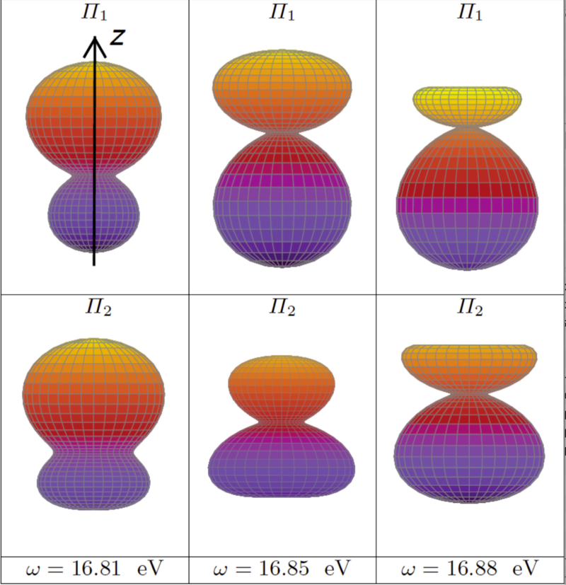
Figure 6: Calculated PADs in the TDSE approach for the pulse $\Pi_{1}$ (top panels) and $\Pi_{2}$ (bottom panels), at three different fundamental frequencies $\omega$ for $\phi=0$. The $z$-axis points upwards through the centers of the panels, as indicated in the top left panel. The distance from the center to a point on the surface is proportional to the probability density for the electron to be ejected along this direction.

Analyzing the results near resonance in Fig. 5, we observe that the TDSE and PT results do not agree as well as for the shorter pulse $\Pi_{1}$, even though the general trend looks similar. There is, however, an explanation for this discrepancy. It can be understood by focusing first on the behavior of $\beta_{4}$. There are two reasons for nonvanishing values of $\beta_{4}$. The first one is direct two-photon ionization into the $f$-wave channel. However, $f$-wave ionization is almost negligible in all calculations presented in this work, and hence interference of the $p$- and $f$- amplitudes only produces small nonzero $\beta_{4}$ values, which are visible in Fig. 4 in the TDSE calculation and also below in Fig. 7. A second, indirect reason for nonzero $\beta_{4}$ values in the present situation is the following: While the second harmonic ionizes neon, the fundamental frequency depletes the $2p$ state over time, especially in the long $\Pi_{2}$ pulse. However, only the $m=0$ magnetic component of the $2p$ state can be pumped to the $3s$ state by the fundamental. As a consequence of the depletion of this sublevel, the second harmonic ionizes an “aligned” $2p$ state, thus leading to significant nonvanishing values of $\beta_{4}$. In our implementation of nonstationary PT, $\beta_{4}\approx 0$ as a result of cancellation of terms associated with different $d$-wave components of a photoelectron emitted from an initially unpolarized target. The second effect, therefore, cannot be accounted for in PT. This explains most of the observed differences between the results from the two approaches.

It is also interesting to visualize the three-dimensional PAD for the two pulses considered. Figure 6 shows the PAD at the resonant frequency ($\omega=16.85$ eV) and for small positive ($\omega=16.88$ eV) and negative ($\omega=16.81$ eV) detunings. For both pulses, the direction of maximum emission along the electric field switches while passing through the resonance. The asymmetry of the PAD is relatively large at the three considered frequencies for $\Pi_{1}$. On the other hand, this asymmetry is less pronounced for $\Pi_{2}$ due to the important contribution from $\beta_{4}$, and the smaller contributions from $\beta_{1}$ and $\beta_{3}$. The maximum electron emission forms an angle of about $145^{\circ}$ with the electric field at the resonance.

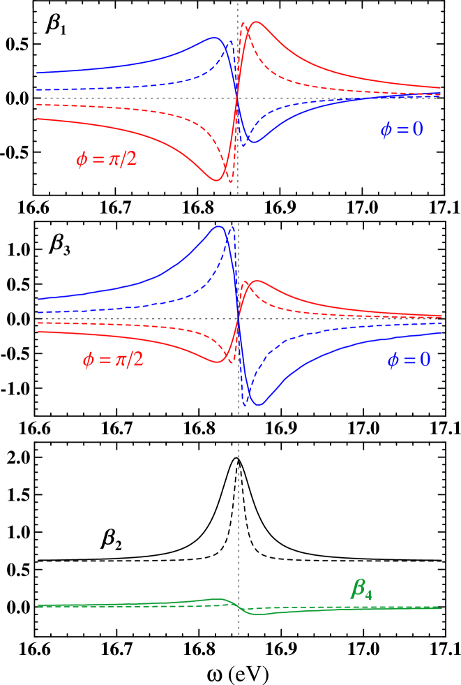
Figure 7: Same as Fig. 4 for the PT-$\infty$ approach with infinite pulse duration and $\eta=0.1$ (solid) and $\eta=\sqrt{0.1}$ (dashed).

The results of the stationary PT-$\infty$ model are presented in Fig. 7 for both amplitude ratios $\eta=0.1$ and $\eta=\sqrt{0.1}$. The different anisotropy parameters vary according to the parametric forms given in Sect. II. Accounting effectively for all intermediate states allows incorporating $f$-wave ionization more accurately in the PT-$\infty$ model than in non-stationary PT. As a result, nonzero, but still small $\beta_{4}$ values appear.

As predicted, the resonance profile is rather sharp for $N=\infty$ and the corresponding resonance would be broader for smaller $\eta$, as seen in Eq. (19). Other features predicted by Eqs. (15)–(22) are very well seen: the odd-rank asymmetry parameters go to zero at the resonance while $\beta_{2}\approx 2$ due to resonant excitation of the intermediate $3s$ state; the amplitude of variations of $\beta_{k}$ ($k=1,\,2,\,3$) are independent of $\eta$. Some of the strong variations of the anisotropy parameters are most likely exaggerated, since in this specific case the population of the $3s$ state assumes significant values, thereby preventing an accurate description based on PT. Nevertheless, it is clear that such a method has a predictive potential, particularly for weak fundamental intensities, as it allows studying the currently realistic experimental situation of rather long FEL pulses. Due to the computational resources required, such long pulses are particularly hard to simulate in the TDSE approach.

An advantage of the PT approach is its ability to study the $\omega+2\,\omega$ process over a large range of pulse parameters with restricted computational resources. Figure 8 shows how the profile of the asymmetry (6) is modified as a function of (a) the number of cycles $N$ and (b) the relative strength of the second harmonic $\eta$. With increasing pulse duration the structures become sharper and more symmetric with respect to the $xy$-plane (maxima and minima are symmetric with respect to the resonance position and tend to be equal), and for pulse durations larger than $N=500$, the weak $2p^{5}(^{2}{\rm P}_{3/2})3s$ resonance becomes visible. This resonance (mainly of $\rm{}^{3}P$ character) is excited very weakly, since it only contains a small ($\approx 7\%$) $\rm{}^{1}P$ component. Nevertheless, when a long pulse is in resonance with $3s$, the interference with the second harmonic is noticeable.

Figure 8b shows how the resonance profile changes with $\eta$. First, for increasing $\eta$ the structure becomes narrower before the amplitude decreases. This is in contradiction with expectations from Eq. (19) and Fig. 7, which predict a constant maximal amplitude. However, for a finite pulse duration ($N=250$) and when $\Gamma_{\beta}$ is smaller than the pulse spectral width, this simple behavior breaks down. For such a short pulse, there is only a small possibility to observe interference with the weak $3s$ resonance: for small $\eta$ the structure is very broad and one cannot distinguish the $(2p^{5}3s)\rm^{1}P_{1}$ resonance from the tale of $(2p^{5}3s)\rm^{3}P_{1}$. If $\eta$ is too large, however, one-photon ionization dominates over the two-photon process, and there is practically no interference.

Finally, we note that within PT decreasing $\eta$ produces the same effect as increasing the total intensity. This is due to the fact that the two-photon ionization amplitudes depend linearly on the intensity while the single-photon amplitude dependence is proportional to $\eta\,\sqrt{I}$. Although the PT simulation cannot be directly extrapolated to higher intensities, Fig. 8 indicates that with increasing intensity the profile of the asymmetry is broadening while its amplitude is decreasing.

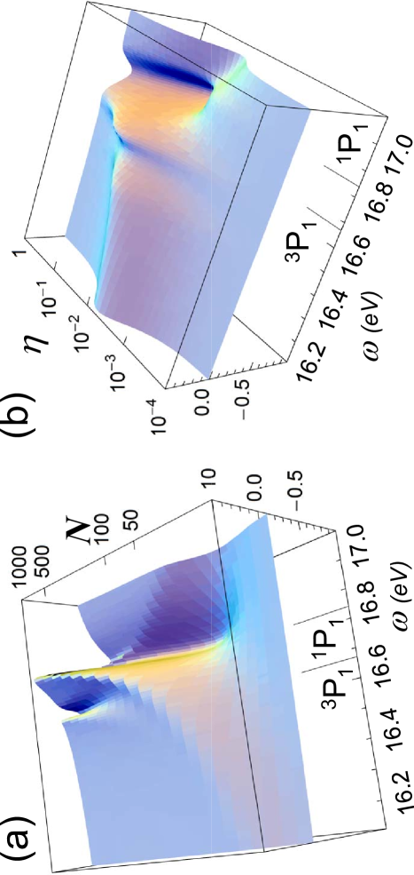
Figure 8: Asymmetry $A(0)$ defined in Eq. (6) for $\phi=0$ as function of energy and number of cycles for $\eta=0.1$ and as function of energy and $\eta$ for $N=250$ (b). The positions of the two $2p^{5}3s$ states with $J=1$ and predominant triplet and singlet character (see text) are indicated.

IV Conclusions and Future Perspectives

We analyzed in detail the ionization by a linearly polarized bichromatic XUV pulse containing the fundamental and the second harmonic ($\omega+2\,\omega$ process) in neon using the $(2p^{5}3s)\;J=1$ states as intermediate states. Two particular situations were considered, corresponding to different pulse lengths and intensities of the second harmonic representing either $1\%$ or $10\%$ of the fundamental. Solving the time-dependent Schrödinger equation as well as employing a perturbative approach, we studied the variations of the photoelectron angular distribution, in particular the anisotropy parameters, as a function of the fundamental frequency.

The results demonstrate that for an intermediate state of a multi-electron system, well separated from other electronic states and well represented in $LS$-coupling, theoretical models based on different approaches can achieve quantitative agreement in describing the characteristics of the $\omega+2\,\omega$ process. We also show that a significant asymmetry can be produced on a wide range of values of the amplitude ratio of the second harmonic over the fundamental. This is an interesting characteristic since the second harmonic admixture can sometimes be difficult to control, or even be estimated, experimentally.

Although results for both approaches agree well for the shorter pulse, noticeable effects beyond the (lowest-order) perturbative approach can appear for longer pulse. In our case, an unexpected resonant behavior of the $\beta_{4}$ parameter in the PAD was revealed through the time-dependent calculations. Nevertheless, the perturbative treatment can reproduce the main trends of the process and allows us to predict its outcomes for a variety of pulse parameters in the relatively weak-field regime, especially for presently realistic experimental conditions, where relatively long pulses are employed.

Since the $\omega+2\,\omega$ process using $(2p^{5}4s)\,J=1$ as intermediate states was investigated experimentally, a thorough theoretical study of this case in the future seems highly desirable. However, this situation presents additional challenges since the intermediate states are not well described in the $LS$-coupling scheme. Furthermore, high-lying discrete Rydberg as well as continuum states might play a significant role.

References

- (1) N. B. Baranova, I. M. Beterov, B. Ya. Zel’dovich, I. I. Ryabtsev, A. N. Chudinov, and A. A. Shul’ginov, Pis’ma Zh. Eksp. Teor. Fiz. 55, 431 (1992) [JETP Lett. 55 439 (1992)]
- (2) Y.-Y. Yin, C. Chen, D. S. Elliott, and A. V. Smith, Phys. Rev. Lett. 69, 2353 (1992).
- (3) N. B. Baranova and B. Ya. Zel dovich, J. Opt. Soc. Am. 8, 27 (1991).
- (4) K. J. Schafer and K. C. Kulander, Phys. Rev. A 45, 8026 (1992).
- (5) Z.-M. Wang and D. S. Elliott, Phys. Rev. Lett. 87, 173001 (2001).
- (6) R. Yamazaki and D. S. Elliott, Phys. Rev. Lett. 98, 053001 (2007); Phys. Rev. A 76, 053401 (2007).
- (7) E. Ehlotzky, Phys. Rep. 345, 175 (2001).
- (8) V. A. Astapenko, Quantum Electron. 36, 1131 (2006).
- (9) Y.-Y. Yin, D. S. Elliott, R. Shehadeh, and E. R. Grant, Chem. Phys. Lett. 241, 591 (1995).
- (10) A. N. Grum-Grzhimailo, E. V. Gryzlova, E. I. Staroselskaya, J. Venzke, and K. Bartschat, Phys. Rev. A 91, 063418 (2015); Erratum: Phys. Rev. A 93, 019901 (2016).
- (11) K. C. Prince et al., Nat. Phot. 10, 176 (2016).
- (12) N. Douguet, A. N. Grum-Grzhimailo, E. V. Gryzlova, E. I. Staroselskaya, J. Venzke, and K. Bartschat, Phys. Rev. A 93, 033402 (2016).
- (13) A. N. Grum-Grzhimailo, A. D. Kondorskiy, and K. Bartschat, J. Phys. B: At. Mol. Opt. Phys. 39, 4659 (2006).
- (14) B. Gao and A. F. Starace, Phys. Rev. Lett. 61, 404 (1988).
- (15) A. E. Orel and T. N. Rescigno, Chem. Phys. Lett. 146, 434 (1988).
- (16) B. Gao, C. Pan, C. R. Liu, and A. F. Starace, J. Opt. Soc. Am. B 7, 622 (1990).
- (17) E. I. Staroselskaya and A. N. Grum-Grzhimailo, Vest. Mosk. Univ. Fiz. N5, 45 (2015) [Moscow Univ. Phys. Bull. 70, 374 (2015)].
- (18) L. E. Machado, P. L. Emerson, and G. Csanak, J. Phys. B: At. Mol. Opt. Phys. 15, 1773 (1982).
- (19) A. Kramida, Yu. Ralchenko, J. Reader, and NIST ASD Team (20l6). NIST Atomic Spectra Database (version 5.4), [Online].
- (20) A. N. Grum-Grzhimailo, B. Abeln, K. Bartschat, D. Weflen, and T. Urness, Phys. Rev. A 81, 043408 (2010).
- (21) C. Froese Fischer, T. Brage, and P. Jönsson 1997 Computational Atomic Structure. An MCHF Approach (IOP Publishing, Bristol, 1997).
- (22) I. I. Sobelman, Introduction to the Theory of Atomic Spectra (Pergamon Press, Oxford, 1972).
- (23) D. A. Varshalovich, A. N. Moskalev, and V. K. Khersonskii, Quantum Theory of Angular Momentum (World Scientific, Singapore, 1988).
- (24) B. Gao and A. F. Starace, Phys. Rev. A 39, 4550 (1989).
- (25) F. Herman and S. Skillman, Atomic Structure Calculations (Prentice-Hall, Englewood Cliffs, N.J., 1963).
- (26) K. Codling, R. G. Houlgate, J. B. West, and P. R. Woodruff, J. Phys. B: At. Mol. Phys. 9, L83 (1976).
- (27) H. Derenbach, R. Malutzki and V. Schmidt, Nucl. Instr. and Meth. 208, 845 (1983).
- (28) V. Schmidt, Z. Phys. D 2, 275 (1986).
- (29) D. J. Kennedy and S. T. Manson, Phys. Rev. A 5, 227 (1972).
- (30) M. Ya. Amusia, N. A. Cherepkov, and L. V. Chernysheva, Phys. Lett. A 40, 15 (1972).
- (31) U. Becker and D. A. Shirley, Partial Cross Sections and Angular Distributions, in VUV and Soft X-Ray Photoionization (Eds. U. Becker, D. A. Shirley; Springer, 1996).
- (32) V. Schmidt, Electron Spectrometry using Synchrotron Radiation (Cambridge University Press, Cambridge, UK, 1997).