Please Lower Small Cell Antenna Heights in 5G

Abstract

In this paper, we present a new and significant theoretical discovery. If the absolute height difference between base station (BS) antenna and user equipment (UE) antenna is larger than zero, then the network capacity performance in terms of the area spectral efficiency (ASE) will continuously decrease as the BS density increases for ultra-dense (UD) small cell networks (SCNs). This performance behavior has a tremendous impact on the deployment of UD SCNs in the 5th-generation (5G) era. Network operators may invest large amounts of money in deploying more network infrastructure to only obtain an even worse network performance. Our study results reveal that it is a must to lower the SCN BS antenna height to the UE antenna height to fully achieve the capacity gains of UD SCNs in 5G. However, this requires a revolutionized approach of BS architecture and deployment, which is explored in this paper too.

I Introduction

From 1950 to 2000, the wireless network capacity has increased around 1 million fold, in which an astounding 2700× gain was achieved through network densification using smaller cells [1]. After 2008, network densification continues to fuel the 3rd Generation Partnership Project (3GPP) 4th-generation (4G) Long Term Evolution (LTE) networks, and is expected to remain as one of the main forces to drive the 5th-generation (5G) networks onward [2]. Indeed, the orthogonal deployment of ultra-dense (UD) small cell networks (SCNs) within the existing macrocell network, i.e., small cells and macrocells operating on different frequency spectrum (3GPP Small Cell Scenario #2a [3]), is envisaged as the workhorse for capacity enhancement in 5G due to its large spectrum reuse and its easy management; the latter one arising from its low interaction with the macrocell tier, e.g., no inter-tier interference [2]. In this paper, the focus is on the analysis of these UD SCNs with an orthogonal deployment with the macrocells.

Before 2015, the common understanding on SCNs was that the density of base stations (BSs) would not affect the per-BS coverage probability performance in interference-limited fully-loaded wireless networks, and thus the area spectral efficiency (ASE) performance in $\textrm{bps/Hz/km}^{2}$ would scale linearly with network densification [4]. The implication of such conclusion is huge: The BS density does NOT matter, since the increase in the interference power caused by a denser network would be exactly compensated by the increase in the signal power due to the reduced distance between transmitters and receivers. Fig. 1 shows the theoretical ASE performance predicted in [4]. However, it is important to note that this conclusion was obtained with considerable simplifications on the propagation environment, which should be placed under scrutiny when evaluating dense and UD SCNs, since they are fundamentally different from sparse ones in various aspects [2].

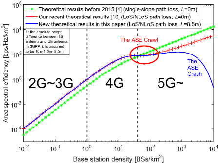
Fig. 1: Theoretical comparison of the ASE performance in $\textrm{bps/Hz/km}^{2}$. Note that all the results are obtained using practical 3GPP channel models [5, 6], which will be explained in details later. Due to the practicality of the used channel models, the results shown here accurately characterize realistic telecommunication systems both qualitatively and quantitatively. For example, considering a typical bandwidth of 10 MHz~100 MHz for the state-of-the-art LTE network, the achievable area throughput is in the order of several $\textrm{Gbps/km}^{2}$, because the ASE for 4G is shown to be around 100 $\textrm{bps/Hz/km}^{2}$.

In the last year, a few noteworthy studies have been carried out to revisit the network performance analysis for UD SCNs under more practical propagation assumptions. In [7], the authors considered a multi-slope piece-wise path loss function, while in [8], the authors investigated line-of-sight (LoS) and non-line-of-sight (NLoS) transmission as a probabilistic event for a millimeter wave communication scenario. The most important finding in these two works was that the per-BS coverage probability performance starts to decrease when the BS density is sufficiently large. Fortunately, such decrease of coverage probability did not change the monotonic increase of the ASE as the BS density increases.

In our very recent work [9, 10], we took a step further and generalized the works in [7] and [8] by considering both piece-wise path loss functions and probabilistic NLoS and LoS transmissions. Our new finding was not only quantitatively but also qualitatively different from previous results in [4, 7, 8]: The ASE will suffer from a slow growth or even a small decrease on the journey from 4G to 5G when the BS density is larger than a threshold. Fig. 1 shows these new theoretical results on the ASE performance, where such threshold is around 20 $\textrm{BSs/km}^{2}$ and the slow/negative ASE growth is highlighted by a circled area. This circled area is referred to as the ASE Crawl hereafter. The intuition of the ASE Crawl is that the interference power increases faster than the signal power due to the transition of a large number of interference paths from NLoS to LoS with the network densification. The implication is profound: The BS density DOES matter, since it affects the signal to interference relationship. Thus, operators should be careful when deploying dense SCNs in order to avoid investing huge amounts of money and end up obtaining an even worse network performance due to the ASE Crawl. Fortunately, our results in [9, 10] also pointed out that the ASE will again grow almost linearly as the network further evolves to an UD one, i.e., $>10^{3}\thinspace\textrm{BSs/km}^{2}$ in Fig. 1. According to our results and considering a 300 MHz bandwidth, if the BS density can go as high as $10^{4}\thinspace\textrm{BSs/km}^{2}$, the problem of the ASE Crawl caused by the NLoS to LoS transition can be overcome, and an area throughput of $10^{3}\thinspace\textrm{Gbps/km}^{2}$ can be achieved, thus opening up an efficient way forward to 5G.

Unfortunately, the NLoS to LoS transition is not the only obstacle to efficient UD SCNs in 5G, and there are more challenges to overcome to get there. In this paper, we present for the first time the serious problem posed by the absolute antenna height difference between SCN base stations (BSs) and user equipments (UEs), and evaluate its impact on UD SCNs by means of a three-dimensional (3D) stochastic geometry analysis (SGA). We made a new and significant theoretical discovery: If the absolute antenna height difference between BSs and UEs, denoted by $L$, is larger than zero, then the ASE performance will continuously decrease as the SCN goes ultra-dense. Fig. 1 illustrates the significance of such theoretical finding with $L=8.5$ m [11]: After the ASE Crawl, the ASE performance only increases marginally (~1.4x) from 109.1 $\textrm{bps/Hz/km}^{2}$ to 149.6 $\textrm{bps/Hz/km}^{2}$ as the BS density goes from $200\thinspace\textrm{BSs/km}^{2}$ to $10^{3}\thinspace\textrm{BSs/km}^{2}$, which is then followed by a continuous and quick fall starting from around $10^{3}\thinspace\textrm{BSs/km}^{2}$. The implication of this result is even more profound than that of the ASE Crawl, since following a traditional deployment with UD SCN BSs deployed at lamp posts or similar heights may dramatically reduce the network performance in 5G. Such decline of ASE in UD SCNs will be referred to as the ASE Crash hereafter, and its fundamental reasons will be explained in details later in this paper.

In order to address this serious problem of the ASE Crash, we further propose to change the traditional BS deployment, and lower the 5G UD SCN BS antenna height to the UE antenna height, so that the ASE behavior of UD SCNs can roll back to our previous results in [10], thus avoiding the ASE Crash. This requires a revolutionized BS deployment approach, which will also be explored in this paper.

The rest of this paper is structured as follows. Section II describes the system model for the 3D SGA. Section III presents our theoretical results on the coverage probability and the ASE performance, while the numerical results are discussed in Section IV, with remarks shedding new light on the revolutionized BS deployment with UE-height antennas. Finally, the conclusions are drawn in Section V.

II System Model

We consider a downlink (DL) cellular network with BSs deployed on a plane according to a homogeneous Poisson point process (HPPP) $\Phi$ of intensity $\lambda$ $\textrm{BSs/km}^{2}$. UEs are Poisson distributed in the considered network with an intensity of $\rho$ $\textrm{UEs/km}^{2}$. Note that $\rho$ is assumed to be sufficiently larger than $\lambda$ so that each BS has at least one associated UE in its coverage [7, 8, 9, 10]. The two-dimensional (2D) distance between a BS and an a UE is denoted by $r$. Moreover, the absolute antenna height difference between a BS and a UE is denoted by $L$. Hence, the 3D distance between a BS and a UE can be expressed as

$$w=\sqrt{r^{2}+L^{2}}.$$ (1)

Following [9, 10], we adopt a very general and practical path loss model, in which the path loss $\zeta\left(w\right)$ associated with distance $w$ is segmented into $N$ pieces written as

$$\zeta\left(w\right)=\begin{cases}\zeta_{1}\left(w\right),&\textrm{when }0\leq w\leq d_{1}\\ \zeta_{2}\left(w\right),&\textrm{when }d_{1}<w\leq d_{2}\\ \vdots&\vdots\\ \zeta_{N}\left(w\right),&\textrm{when }w>d_{N-1}\end{cases},$$ (2)

where each piece $\zeta_{n}\left(w\right),n\in\left\{1,2,\ldots,N\right\}$ is modeled as

$$\zeta_{n}\left(w\right)=\begin{cases}\begin{array}[]{l}\zeta_{n}^{\textrm{L}}\left(w\right)=A_{n}^{{\rm{L}}}w^{-\alpha_{n}^{{\rm{L}}}},\\ \zeta_{n}^{\textrm{NL}}\left(w\right)=A_{n}^{{\rm{NL}}}w^{-\alpha_{n}^{{\rm{NL}}}},\end{array}&\begin{array}[]{l}\textrm{LoS:}\leavevmode\nobreak\ \textrm{Pr}_{n}^{\textrm{L}}\left(w\right)\\ \textrm{NLoS:}\leavevmode\nobreak\ 1-\textrm{Pr}_{n}^{\textrm{L}}\left(w\right)\end{array},\end{cases}$$ (3)

where $\zeta_{n}^{\textrm{L}}\left(w\right)$ and $\zeta_{n}^{\textrm{NL}}\left(w\right),n\in\left\{1,2,\ldots,N\right\}$ are the $n$-th piece path loss functions for the LoS transmission and the NLoS transmission, respectively, $A_{n}^{{\rm{L}}}$ and $A_{n}^{{\rm{NL}}}$ are the path losses at a reference distance $w=1$ for the LoS and the NLoS cases, respectively, and $\alpha_{n}^{{\rm{L}}}$ and $\alpha_{n}^{{\rm{NL}}}$ are the path loss exponents for the LoS and the NLoS cases, respectively. In practice, $A_{n}^{{\rm{L}}}$, $A_{n}^{{\rm{NL}}}$, $\alpha_{n}^{{\rm{L}}}$ and $\alpha_{n}^{{\rm{NL}}}$ are constants obtainable from field tests [5, 6]. Moreover, $\textrm{Pr}_{n}^{\textrm{L}}\left(w\right)$ is the $n$-th piece LoS probability function that a transmitter and a receiver separated by a distance $w$ has a LoS path, which is assumed to be a monotonically decreasing function with regard to $w$.

For convenience, $\left\{\zeta_{n}^{\textrm{L}}\left(w\right)\right\}$ and $\left\{\zeta_{n}^{\textrm{NL}}\left(w\right)\right\}$ are further stacked into piece-wise functions written as

$$\zeta^{Path}\left(w\right)=\begin{cases}\zeta_{1}^{Path}\left(w\right),&\textrm{when }0\leq w\leq d_{1}\\ \zeta_{2}^{Path}\left(w\right),&\textrm{when }d_{1}<w\leq d_{2}\\ \vdots&\vdots\\ \zeta_{N}^{Path}\left(w\right),&\textrm{when }w>d_{N-1}\end{cases},$$ (4)

where the string variable $Path$ takes the value of “L” and “NL” for the LoS and the NLoS cases, respectively.

Besides, $\left\{\textrm{Pr}_{n}^{\textrm{L}}\left(w\right)\right\}$ is stacked into a piece-wise function as

$$\textrm{Pr}^{\textrm{L}}\left(w\right)=\begin{cases}\textrm{Pr}_{1}^{\textrm{L}}\left(w\right),&\textrm{when }0\leq w\leq d_{1}\\ \textrm{Pr}_{2}^{\textrm{L}}\left(w\right),&\textrm{when }d_{1}<w\leq d_{2}\\ \vdots&\vdots\\ \textrm{Pr}_{N}^{\textrm{L}}\left(w\right),&\textrm{when }w>d_{N-1}\end{cases}.$$ (5)

In this paper, we assume a practical user association strategy (UAS), in which each UE should be associated with the BS providing the smallest path loss (i.e., with the largest $\zeta\left(w\right)$) [8, 10]. In addition, we assume that each BS/UE is equipped with an isotropic antenna, and that the multi-path fading between a BS and a UE is modeled as independently identical distributed (i.i.d.) Rayleigh fading [7, 8, 9, 10]. Note that a more practical Rician fading will also be considered in the simulation section to show its impact on our conclusions.

III Main Results

Using a 3D SGA based on the HPPP theory, we study the performance of the SCN by considering the performance of a typical UE located at the origin $o$.

We first investigate the coverage probability that this UE’s signal-to-interference-plus-noise ratio (SINR) is above a per-designated threshold $\gamma$:

$$p^{\textrm{cov}}\left(\lambda,\gamma\right)=\textrm{Pr}\left[\mathrm{SINR}>\gamma\right],$$ (6)

where the SINR is calculated as

$$\mathrm{SINR}=\frac{P\zeta\left(w\right)h}{I_{\textrm{agg}}+N_{0}},$$ (7)

where $h$ is the channel gain and is modeled as an exponential random variable (RV) with the mean of one due to Rayleigh fading, $P$ and $N_{0}$ are the transmission power of each BS and the additive white Gaussian noise (AWGN) power at each UE, respectively, and $I_{\textrm{agg}}$ is the cumulative interference given by

$$I_{\textrm{agg}}=\sum_{i:\,b_{i}\in\Phi\setminus b_{o}}P\beta_{i}g_{i},$$ (8)

where $b_{o}$ is the BS serving the typical UE located at distance $w$ from the typical UE, and $b_{i}$, $\beta_{i}$ and $g_{i}$ are the $i$-th interfering BS, the path loss associated with $b_{i}$ and the multi-path fading channel gain associated with $b_{i}$, respectively.

Based on the path loss model in (2) with 3D distances and the considered UAS, we present our main result on $p^{\textrm{cov}}\left(\lambda,\gamma\right)$ in Theorem 1 shown on the top of the next page.

Theorem 1.

Considering the path loss model in (2) and the presented UAS, the probability of coverage $p^{{\rm{cov}}}\left(\lambda,\gamma\right)$ can be derived as

$$p^{{\rm{cov}}}\left(\lambda,\gamma\right)=\sum_{n=1}^{N}\left(T_{n}^{{\rm{L}}}+T_{n}^{{\rm{NL}}}\right),$$ (9)

where $T_{n}^{{\rm{L}}}=\int_{\sqrt{d_{n-1}^{2}-L^{2}}}^{\sqrt{d_{n}^{2}-L^{2}}}{\rm{Pr}}\left[\frac{P\zeta_{n}^{{\rm{L}}}\left(\sqrt{r^{2}+L^{2}}\right)h}{I_{{\rm{agg}}}+N_{0}}>\gamma\right]f_{R,n}^{{\rm{L}}}\left(r\right)dr$, $T_{n}^{{\rm{NL}}}=\int_{\sqrt{d_{n-1}^{2}-L^{2}}}^{\sqrt{d_{n}^{2}-L^{2}}}{\rm{Pr}}\left[\frac{P\zeta_{n}^{{\rm{NL}}}\left(\sqrt{r^{2}+L^{2}}\right)h}{I_{{\rm{agg}}}+N_{0}}>\gamma\right]f_{R,n}^{{\rm{NL}}}\left(r\right)dr$, and $d_{0}$ and $d_{N}$ are defined as $L$ and $+\infty$, respectively. Moreover, $f_{R,n}^{{\rm{L}}}\left(r\right)$ and $f_{R,n}^{{\rm{NL}}}\left(r\right)$ $\left(\sqrt{d_{n-1}^{2}-L^{2}}<r\leq\sqrt{d_{n}^{2}-L^{2}}\right)$, are represented by

$$f_{R,n}^{{\rm{L}}}\left(r\right)=\exp\left(-\int_{0}^{r_{1}}\left(1-{\rm{Pr}}^{{\rm{L}}}\left(\sqrt{u^{2}+L^{2}}\right)\right)2\pi u\lambda du\right)\exp\left(-\int_{0}^{r}{\rm{Pr}}^{{\rm{L}}}\left(\sqrt{u^{2}+L^{2}}\right)2\pi u\lambda du\right){\rm{Pr}}_{n}^{{\rm{L}}}\left(\sqrt{r^{2}+L^{2}}\right)2\pi r\lambda,$$ (10)

and

$$f_{R,n}^{{\rm{NL}}}\left(r\right)=\exp\left(-\int_{0}^{r_{2}}{\rm{Pr}}^{{\rm{L}}}\left(\sqrt{u^{2}+L^{2}}\right)2\pi u\lambda du\right)\exp\left(-\int_{0}^{r}\left(1-{\rm{Pr}}^{{\rm{L}}}\left(\sqrt{u^{2}+L^{2}}\right)\right)2\pi u\lambda du\right)\left(1-{\rm{Pr}}_{n}^{{\rm{L}}}\left(\sqrt{r^{2}+L^{2}}\right)\right)2\pi r\lambda,$$ (11)

where $r_{1}$ and $r_{2}$ are given implicitly by the following equations as

$$r_{1}=\underset{r_{1}}{\arg}\left\{\zeta^{{\rm{NL}}}\left(\sqrt{r_{1}^{2}+L^{2}}\right)=\zeta_{n}^{{\rm{L}}}\left(\sqrt{r^{2}+L^{2}}\right)\right\},$$ (12)

and

$$r_{2}=\underset{r_{2}}{\arg}\left\{\zeta^{{\rm{L}}}\left(\sqrt{r_{2}^{2}+L^{2}}\right)=\zeta_{n}^{{\rm{NL}}}\left(\sqrt{r^{2}+L^{2}}\right)\right\}.$$ (13)

In addition, ${\rm{Pr}}\left[\frac{P\zeta_{n}^{{\rm{L}}}\left(\sqrt{r^{2}+L^{2}}\right)h}{I_{{\rm{agg}}}+N_{0}}>\gamma\right]$ and ${\rm{Pr}}\left[\frac{P\zeta_{n}^{{\rm{NL}}}\left(\sqrt{r^{2}+L^{2}}\right)h}{I_{{\rm{agg}}}+N_{0}}>\gamma\right]$ are respectively computed by

$${\rm{Pr}}\left[\frac{P\zeta_{n}^{{\rm{L}}}\left(\sqrt{r^{2}+L^{2}}\right)h}{I_{{\rm{agg}}}+N_{0}}>\gamma\right]=\exp\left(-\frac{\gamma N_{0}}{P\zeta_{n}^{{\rm{L}}}\left(\sqrt{r^{2}+L^{2}}\right)}\right)\mathscr{L}_{I_{{\rm{agg}}}}^{{\rm{L}}}\left(\frac{\gamma}{P\zeta_{n}^{{\rm{L}}}\left(\sqrt{r^{2}+L^{2}}\right)}\right),$$ (14)

where $\mathscr{L}_{I_{{\rm{agg}}}}^{{\rm{L}}}\left(s\right)$ is the Laplace transform of $I_{{\rm{agg}}}$ for LoS signal transmission evaluated at $s$, which can be further written as

$$\mathscr{L}_{I_{{\rm{agg}}}}^{{\rm{L}}}\left(s\right)=\exp\left(-2\pi\lambda\int_{r}^{+\infty}\frac{{\rm{Pr}}^{{\rm{L}}}\left(\sqrt{u^{2}+L^{2}}\right)u}{1+\left(sP\zeta^{{\rm{L}}}\left(\sqrt{u^{2}+L^{2}}\right)\right)^{-1}}du\right)\exp\left(-2\pi\lambda\int_{r_{1}}^{+\infty}\frac{\left[1-{\rm{Pr}}^{{\rm{L}}}\left(\sqrt{u^{2}+L^{2}}\right)\right]u}{1+\left(sP\zeta^{{\rm{NL}}}\left(\sqrt{u^{2}+L^{2}}\right)\right)^{-1}}du\right),$$ (15)

and

$${\rm{Pr}}\left[\frac{P\zeta_{n}^{{\rm{NL}}}\left(\sqrt{r^{2}+L^{2}}\right)h}{I_{{\rm{agg}}}+N_{0}}>\gamma\right]=\exp\left(-\frac{\gamma N_{0}}{P\zeta_{n}^{{\rm{NL}}}\left(\sqrt{r^{2}+L^{2}}\right)}\right)\mathscr{L}_{I_{{\rm{agg}}}}^{{\rm{NL}}}\left(\frac{\gamma}{P\zeta_{n}^{{\rm{NL}}}\left(\sqrt{r^{2}+L^{2}}\right)}\right),$$ (16)

where $\mathscr{L}_{I_{{\rm{agg}}}}^{{\rm{NL}}}\left(s\right)$ is the Laplace transform of $I_{{\rm{agg}}}$ for NLoS signal transmission evaluated at $s$, which can be further written as

$$\mathscr{L}_{I_{{\rm{agg}}}}^{{\rm{NL}}}\left(s\right)=\exp\left(-2\pi\lambda\int_{r_{2}}^{+\infty}\frac{{\rm{Pr}}^{{\rm{L}}}\left(\sqrt{u^{2}+L^{2}}\right)u}{1+\left(sP\zeta^{{\rm{L}}}\left(\sqrt{u^{2}+L^{2}}\right)\right)^{-1}}du\right)\exp\left(-2\pi\lambda\int_{r}^{+\infty}\frac{\left[1-{\rm{Pr}}^{{\rm{L}}}\left(\sqrt{u^{2}+L^{2}}\right)\right]u}{1+\left(sP\zeta^{{\rm{NL}}}\left(\sqrt{u^{2}+L^{2}}\right)\right)^{-1}}du\right).$$ (17)

Proof:

We omit the proof here due to the page limitation. We will provide the full proof in the journal version of this paper. ∎

According to [9, 10], we also investigate the ASE in $\textrm{bps/Hz/km}^{2}$ for a given $\lambda$, which can be computed as

$$A^{\textrm{ASE}}\left(\lambda,\gamma_{0}\right)=\lambda\int_{\gamma_{0}}^{+\infty}\log_{2}\left(1+\gamma\right)f_{\mathit{\Gamma}}\left(\lambda,\gamma\right)d\gamma,$$ (18)

where $\gamma_{0}$ is the minimum working SINR for the considered SCN, and $f_{\mathit{\Gamma}}\left(\lambda,\gamma\right)$ is the probability density function (PDF) of the SINR observed at the typical UE at a particular value of $\lambda$. Based on the definition of $p^{\textrm{cov}}\left(\lambda,\gamma\right)$ in (6), which is the complementary cumulative distribution function (CCDF) of SINR, $f_{\mathit{\Gamma}}\left(\lambda,\gamma\right)$ can be expressed by

$$f_{\mathit{\Gamma}}\left(\lambda,\gamma\right)=\frac{\partial\left(1-p^{\textrm{cov}}\left(\lambda,\gamma\right)\right)}{\partial\gamma},$$ (19)

where $p^{\textrm{cov}}\left(\lambda,\gamma\right)$ is obtained from Theorem 1.

Considering the results of $p^{\textrm{cov}}\left(\lambda,\gamma\right)$ and $A^{\textrm{ASE}}\left(\lambda,\gamma_{0}\right)$ respectively shown in (9) and (18), we propose Theorem 2 to theoretically explain the fundamental reasons of the ASE Crash discussed in Section I.

Theorem 2.

If $L>0$ and $\gamma,\gamma_{0}<+\infty$, then $\underset{\lambda\rightarrow+\infty}{\lim}p^{{\rm{cov}}}\left(\lambda,\gamma\right)=0$ and $\underset{\lambda\rightarrow+\infty}{\lim}A^{{\rm{ASE}}}\left(\lambda,\gamma_{0}\right)=0$.

Proof:

We omit the proof here due to the page limitation. Instead, in the following, we describe the essence of theorem and provide a toy example to clarify it. We will provide the full proof in the journal version of this paper. ∎

In essence, Theorem 2 states that when $\lambda$ is extremely large, e.g., in UD SCNs, both $p^{\textrm{cov}}\left(\lambda,\gamma\right)$ and $A^{\textrm{ASE}}\left(\lambda,\gamma_{0}\right)$ will decrease towards zero with the network densification, and UEs will experience service outage, thus creating the ASE Crash. The fundamental reason for this phenomenon is revealed by the key point of the proof, i.e., the signal power will lose its superiority over the interference power when $\lambda\rightarrow+\infty$, even if the interference created by the BSs that are relatively far away is ignored. This is because the absolute antenna height difference $L$ introduces a cap on the signal-link distance and thus on the signal power. Theorem 2 is in stark contrast with the conclusion in [4, 7, 8, 9, 10], which indicates that the increase in the interference power will be exactly counter-balanced by the increase in the signal power when $\lambda\rightarrow+\infty$.

Since the proof of Theorem 2 is mathematically intense and difficult to digest, in the following we provide a toy example to shed some valuable insights on the rationale behind Theorem 2. We consider a simple 2-BS SCN as illustrated in Fig. 2, where the 2D distance between the serving BS and the UE and that between an arbitrary interfering BS and the UE are denoted by $r$ and $\tau r,\left(1<\tau<+\infty\right)$, respectively. In this example, when $\lambda\rightarrow+\infty$, then $r\rightarrow 0$, which can be intuitively explained by the fact that the per-BS coverage area is roughly in the order of $\frac{1}{\lambda}$, and thus the typical 2D distance from the serving BS to the UE approaches zero when $\lambda\rightarrow+\infty$.

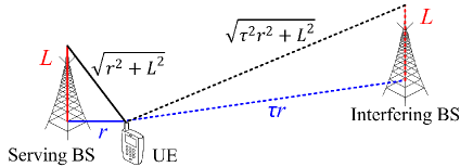
Fig. 2: Illustration of a toy example with a 2-BS SCN.

Considering that $r\rightarrow 0$ and $L$ is smaller than $d_{1}$ in practical SCNs [6, 5], we can assume that both the signal link and the interference link should be dominantly characterized by the first-piece LoS path loss function in (3), i.e., $\zeta_{1}^{\textrm{L}}\left(w\right)=A_{1}^{{\rm{L}}}\left(\sqrt{r^{2}+L^{2}}\right)^{-\alpha_{1}^{{\rm{L}}}}$. Thus, based on the 3D distances, we can obtain the signal-to-interference ratio (SIR) as

$$\bar{\gamma}=\frac{A_{1}^{{\rm{L}}}\left(\sqrt{r^{2}+L^{2}}\right)^{-\alpha_{1}^{{\rm{L}}}}}{A_{1}^{{\rm{L}}}\left(\sqrt{\tau^{2}r^{2}+L^{2}}\right)^{-\alpha_{1}^{{\rm{L}}}}}=\left(\sqrt{\frac{1}{1+\frac{\tau^{2}-1}{1+\frac{L^{2}}{r^{2}}}}}\right)^{-\alpha_{1}^{{\rm{L}}}}.$$ (20)

Note that $\bar{\gamma}$ is a monotonically decreasing function as $r$ decreases when $L>0$. Moreover, it is easy to show that

$$\underset{\lambda\rightarrow+\infty}{\lim}\bar{\gamma}=\underset{r\rightarrow 0}{\lim}\bar{\gamma}=\begin{cases}\begin{array}[]{l}1,\\ \tau^{\alpha_{1}^{{\rm{L}}}},\end{array}&\begin{array}[]{l}\left(L>0\right)\\ \left(L=0\right)\end{array}.\end{cases}$$ (21)

Assuming that $\tau=10$ and $\alpha_{1}^{{\rm{L}}}=2$ in (21), the limit of $\bar{\gamma}$ in UD SCNs will plunge from 20 dB when $L=0$ to 0 dB when $L>0$, which means that even a rather weak interferer, e.g., with a power 20 dB below the signal power, will become a real threat to the signal link when the absolute antenna height difference $L$ is non-zero in UD SCNs. The drastic crash of $\bar{\gamma}$ when $L>0$ is due to the cap imposed on the signal power as the signal-link distance $\sqrt{r^{2}+L^{2}}$ in the numerator of (20) cannot go below $L$. Such cap on the signal-link distance and the signal power leads to the ASE Crash, since other signal-power-comparable interferers also approach the UE from all directions as $\lambda$ increases, which will eventually cause service outage to the UE.

To sum up, in an UD SCN with conventional deployment (i.e., $L>0$), both $p^{\textrm{cov}}\left(\lambda,\gamma\right)$ and $A^{\textrm{ASE}}\left(\lambda,\gamma_{0}\right)$ will plunge toward zero as $\lambda$ increases, causing the ASE Crash. Its fundamental reason is the cap on the signal power because of the minimum signal-link distance tied to $L$, which cannot be overcome with the densification. The only way to avoid the ASE Crash is to remove the signal power cap by setting $L$ to zero, which means lowering the BS antenna height, not just by a few meters, but straight to the UE antenna height. Other applicable solutions may be the usage of very directive antennas and/or the usage of sophisticated idle modes at the SCN BSs, which will be investigated in our future work.

IV Simulation and Discussion

In this section, we investigate the network performance and use numerical results to establish the accuracy of our analysis.

As a special case of Theorem 1, following [10], we consider a two-piece path loss and a linear LoS probability functions defined by the 3GPP [5, 6]. Specifically, in the path loss model presented in (2), we use $N=2$, $\zeta_{1}^{\textrm{L}}\left(w\right)=\zeta_{2}^{\textrm{L}}\left(w\right)=A^{{\rm{L}}}w^{-\alpha^{{\rm{L}}}}$, $\zeta_{1}^{\textrm{NL}}\left(w\right)=\zeta_{2}^{\textrm{NL}}\left(w\right)=A^{{\rm{NL}}}w^{-\alpha^{{\rm{NL}}}}$ [5]. And in the LoS probability model shown in (5), we use $\textrm{Pr}_{1}^{\textrm{L}}\left(w\right)=1-\frac{w}{d_{1}}$ and $\textrm{Pr}_{2}^{\textrm{L}}\left(w\right)=0$, where $d_{1}$ is a constant [6]. For clarity, this 3GPP special case is referred to as 3GPP Case 1. As justified in [10], we use 3GPP Case 1 for the case study because it provides tractable results for (10)-(17) in Theorem 1. The details are relegated to the journal version of this paper.

Following [10], we adopt the following parameters for 3GPP Case 1: $d_{1}=300$ m, $\alpha^{{\rm{L}}}=2.09$, $\alpha^{{\rm{NL}}}=3.75$, $A^{{\rm{L}}}=10^{-10.38}$, $A^{{\rm{NL}}}=10^{-14.54}$, $P=24$ dBm, $N_{0}=-95$ dBm. The BS antenna and the UE antenna heights are set to 10 m and 1.5 m, respectively [11], thus $L=\left|10-1.5\right|=8.5$ m.

To check the impact of different path loss models on our conclusions, we have also investigated the results for a single-slope path loss model that does not differentiate LoS and NLoS transmissions [4], where only one path loss exponent $\alpha$ is defined, the value of which is assumed to be $\alpha=\alpha^{{\rm{NL}}}=3.75$.

IV-A Validation of Theorem 1 on the Coverage Probability

Fig. 3: $p^{\textrm{cov}}\left(\lambda,\gamma\right)$ vs. $\lambda$ with $\gamma=0\,\textrm{dB}$.

In Fig. 3, we show the results of $p^{\textrm{cov}}\left(\lambda,\gamma\right)$ with $\gamma=0\,\textrm{dB}$. As can be observed from Fig. 3, our analytical results given by Theorem 1 match the simulation results very well, which validates the accuracy of our theoretical analysis. From Fig. 3, we can draw the following observations which are inline with our discussion in Section I:

• For the single-slope path loss model with $L=0$ m, the BS density does NOT matter, since the coverage probability approaches a constant for UD SCNs [4].

• For the 3GPP Case 1 path loss model with $L=0$ m, the BS density DOES matter, since that coverage probability will decrease as $\lambda$ increases when the network is dense enough, e.g., $\lambda>20\,\textrm{BSs/km}^{2}$, due to the transition of a large number of interference paths from NLoS to LoS [10]. When $\lambda$ is tremendously large, e.g., $\lambda\geq 10^{3}\,\textrm{BSs/km}^{2}$, the coverage probability decreases at a slower pace because both the interference and the signal powers are LoS dominated, and thus the coverage probability approaches a constant related to $\alpha^{{\rm{L}}}$ [4, 10].

• For both path loss models, when $L=8.5$ m, the coverage probability shows a determined trajectory toward zero in UD SCNs due to the cap on the signal power introduced by the non-zero $L$ as explained in Theorem 2. In more detail, for the 3GPP Case 1 path loss model with $\lambda=10^{4}\thinspace\textrm{BSs/km}^{2}$, the coverage probability decreases from 0.15 when $L=0$ m to around $10^{-5}$ when $L=8.5$ m.

IV-B The Theoretical Results of the ASE

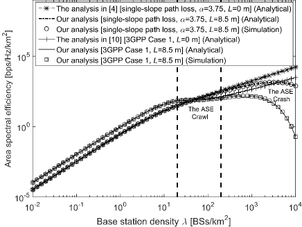
Fig. 4: $A^{\textrm{ASE}}\left(\lambda,\gamma_{0}\right)$ vs. $\lambda$ with $\gamma_{0}=0\,\textrm{dB}$.

In Fig. 4, we show the results of $A^{\textrm{ASE}}\left(\lambda,\gamma_{0}\right)$ with $\gamma_{0}=0\,\textrm{dB}$. Fig. 4 is essentially the same as Fig. 1 with the same marker styles, except that the results for the single-slope path loss model with $L=8.5$ m are also plotted. From Fig. 4, we can confirm the key observations presented in Section I:

• For the single-slope path loss model with $L=0$ m, the ASE performance scales linearly with $\lambda$ [4]. The result is promising, but it might not be the case in reality.

• For the 3GPP Case 1 path loss model with $L=0$ m, the ASE suffers from a slow growth or even a small decrease when $\lambda\in\left[20,200\right]\,\textrm{BSs/km}^{2}$, i.e., the ASE Crawl [10]. After the ASE Crawl, the ASE grows almost linearly again as the network further evolves to an UD one, e.g., $\lambda>10^{3}\thinspace\textrm{BSs/km}^{2}$ [10].

• For both path loss models with $L=8.5$ m, the ASE suffers from severe performance loss in UD SCNs due to the ASE Crash, as explained in Theorem 2. In more detail, for the 3GPP Case 1 path loss model with $\lambda=10^{4}\thinspace\textrm{BSs/km}^{2}$, the ASE dramatically decreases from $3141\thinspace\textrm{bps/Hz/km}^{2}$ when $L=0$ m to $0.2\thinspace\textrm{bps/Hz/km}^{2}$ when $L=8.5$ m.

IV-C Factors that May Impact the ASE Crash

There are several factors that may have large impacts on the existence/severity of the ASE Crash, e.g., various values of $L$ and $\alpha^{{\rm{L}}}$, Rician fading, etc. In Fig. 5, we investigate the performance of $A^{\textrm{ASE}}\left(\lambda,\gamma_{0}\right)$ for 3GPP Case 1 under the assumptions of $L=3.5$ m [3] or $\alpha^{{\rm{L}}}=1.09$ [10] or Rician fading [6]. Due to the significant accuracy of our analysis, we only show analytical results of $A^{\textrm{ASE}}\left(\lambda,\gamma_{0}\right)$ in Fig. 5.

Our key conclusions are summarized as follows:

• Decreasing $L$ from 8.5 m to 3.5 m (BS antenna height being 5 m) helps to alleviate, but cannot remove the ASE Crash unless $L=0$, as explained in Theorem 2. From Fig. 5, the ASE with $L=3.5$ m peaks at around $\lambda=3000\thinspace\textrm{BSs/km}^{2}$, but it still suffers from a 60 % loss compared with the ASE with $L=0$ m at that BS density.

• Decreasing $\alpha^{{\rm{L}}}$ helps to alleviate the ASE Crash because it softens the SIR crash in (21). However, it aggravates the ASE Crawl by showing an obvious ASE decrease when $\lambda\in\left[20,80\right]\,\textrm{BSs/km}^{2}$ due to the drastic interference transition from NLoS to stronger LoS with $\alpha^{{\rm{L}}}=1.09$ [10].

• From the simulation results, we can see that Rician fading makes the ASE Crash worse, which takes effect early from around $\lambda=400\thinspace\textrm{BSs/km}^{2}$. The intuition is that the randomness in channel fluctuation associated with Rician fading is much weaker than that associated with Rayleigh fading due to the large $K$ factor in UD SCNs [6]. With Rayleigh fading, some UE in outage might be opportunistically saved by favorable channel fluctuation of the signal power, while with Rician fading, such outage case becomes more deterministic due to lack of channel variation, thus leading to a severer ASE Crash.

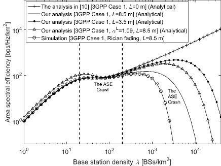
Fig. 5: $A^{\textrm{ASE}}\left(\lambda,\gamma_{0}\right)$ vs. $\lambda$ with $\gamma_{0}=0\,\textrm{dB}$ and various assumptions.

IV-D A Novel BS Deployment with UE-Height Antennas

Based on our thought-provoking discovery, we make the following recommendation to vendors and operators around the world: The SCN BS antenna height must be lowered to the UE antenna height in 5G UD SCNs, so that the ASE behavior of such networks would roll back to our previous results in [9, 10], thus avoiding the ASE Crash. Such proposed new BS deployment will allow to realize the potential gains of UD SCNs, but needs a revolution on BS architectures and network deployment in 5G. The new R&D challenges in this area are:

1. New BS architectures that are anti-vandalism/anti-theft/anti-hacking at low-height positions.

2. Measurement campaigns for the UE-height channels. Note that at such height there is an unusual concentration of objects, such as cars, foliage, etc.

3. Implications of fast time-variant shadow fading due to random movement of UE-height objects, e.g., cars.

4. Terrain-dependent network performance analysis.

5. New inter-BS communications based on ground waves.

6. For macrocell BSs with a large $L$, whose BS antenna height cannot be lowered to the UE antenna height, the existing network performance analysis for heterogeneous networks may need to be revisited, since the interference from the macrocell tier to the SCN tier may have been greatly over-estimated due to the common assumption of $L=0$.

V Conclusion

We presented a new and significant theoretical discovery, i.e., the serious problem of the ASE Crash. If the absolute height difference between BS antenna and UE antenna is larger than zero, then the ASE performance will continuously decrease with network densification for UD SCNs. The only way to fully overcome the ASE Crash is to lower the SCN BS antenna height to the UE antenna height, which will revolutionize the approach of BS architecture and deployment in 5G. In our future work, we will also study how the usage of very directive antennas and/or the usage of sophisticated idle modes at the small cell BSs can help to mitigate the ASE Crash.

References

- [1] ArrayComm & William Webb, Ofcom, London, U.K., 2007.
- [2] D. L pez-P rez, M. Ding, H. Claussen, and A. Jafari, “Towards 1 Gbps/UE in cellular systems: Understanding ultra-dense small cell deployments,” IEEE Communications Surveys Tutorials, vol. 17, no. 4, pp. 2078–2101, Jun. 2015.
- [3] 3GPP, “TR 36.872: Small cell enhancements for E-UTRA and E-UTRAN - Physical layer aspects,” Dec. 2013.
- [4] J. Andrews, F. Baccelli, and R. Ganti, “A tractable approach to coverage and rate in cellular networks,” IEEE Transactions on Communications, vol. 59, no. 11, pp. 3122–3134, Nov. 2011.
- [5] 3GPP, “TR 36.828: Further enhancements to LTE Time Division Duplex (TDD) for Downlink-Uplink (DL-UL) interference management and traffic adaptation,” Jun. 2012.
- [6] Spatial Channel Model AHG, “Subsection 3.5.3, Spatial Channel Model Text Description V6.0,” Apr. 2003.
- [7] X. Zhang and J. Andrews, “Downlink cellular network analysis with multi-slope path loss models,” IEEE Transactions on Communications, vol. 63, no. 5, pp. 1881–1894, May 2015.
- [8] T. Bai and R. Heath, “Coverage and rate analysis for millimeter-wave cellular networks,” IEEE Transactions on Wireless Communications, vol. 14, no. 2, pp. 1100–1114, Feb. 2015.
- [9] M. Ding, D. L pez-P rez, G. Mao, P. Wang, and Z. Lin, “Will the area spectral efficiency monotonically grow as small cells go dense?” IEEE GLOBECOM 2015, pp. 1–7, Dec. 2015.
- [10] M. Ding, P. Wang, D. L pez-P rez, G. Mao, and Z. Lin, “Performance impact of LoS and NLoS transmissions in dense cellular networks,” IEEE Transactions on Wireless Communications, vol. 15, no. 3, pp. 2365–2380, Mar. 2016.
- [11] 3GPP, “TR 36.814: Further advancements for E-UTRA physical layer aspects (Release 9),” Mar. 2010.