Topological properties of spaces admitting a coaxial homeomorphism

Abstract.

Wright [Wri92] showed that, if a 1-ended simply connected locally compact ANR $Y$ with pro-monomorphic fundamental group at infinity (i.e. representable by an inverse sequence of monomorphisms) admits a $\mathbb{Z}$-action by covering transformations, then that fundamental group at infinity can be represented by an inverse sequence of finitely generated free groups. Geoghegan and Guilbault [GG12] strengthened that result, proving that $Y$ also satisfies the crucial semistability condition (i.e. representable by an inverse sequence of epimorphisms).

Here we get a stronger theorem with weaker hypotheses. We drop the “pro-monomorphic hypothesis” and simply assume that the $\mathbb{Z}$-action is generated by what we call a “coaxial” homeomorphism. In the pro-monomorphic case every $\mathbb{Z}$-action by covering transformations is generated by a coaxial homeomorphism, but coaxials occur in far greater generality (often embedded in a cocompact action). When the generator is coaxial, we obtain the sharp conclusion: $Y$ is proper 2-equivalent to the product of a locally finite tree with $\mathbb{R}$. Even in the pro-monomorphic case this is new: it says that, from the viewpoint of fundamental group at infinity, the “end” of $Y$ looks like the suspension of a totally disconnected compact set.

Let $Y$ be a simply connected, locally compact, absolute neighborhood retract (ANR). (Recall that the class of ANR’s includes such familiar and important spaces as topological manifolds and locally finite $CW$ complexes.) Let $\{C_{n}\}$ be an expanding sequence of compact subsets which exhausts $Y$ in the sense that the union of the sets $C_{n}$ is the whole space. The algebraic topology of $Y$ at infinity is studied by means of the inverse sequence of spaces $\{Y-C_{n}\}$ where the bonds are inclusion maps. So, for example, information about the $m^{\text{th}}$ homology of $Y$ at infinity would be obtained from the inverse sequence of abelian groups $\{H_{m}(Y-C_{n})\}$. As a second example, the components at infinity are the ends of $Y$, by which is meant (roughly) the members of the inverse sequence of sets $\{{\pi}_{0}(Y-C_{n})\}$. All this is well-known.

We always assume that $Y$ is simply connected. To keep things simple we assume in this introduction only that $Y$ has one end.

The equivariant case: Suppose, in particular, that a group $G$ acts cocompactly as covering transformations on $Y$ (this implies that $G$ is finitely presented). Then, with suitable extra assumptions, the topological invariants of $Y$ at infinity are invariants of the group $G$. The earliest example is the number of ends of $Y$ which is a feature of $G$, independent of the choice of $Y$; it is a classical theorem of Hopf that this number is $0,1,2$ or $\infty$.

In this paper we add to the current understanding of the fundamental group at infinity of $Y$, motivated particularly by the equivariant case. Pick a proper ray $\omega:[0,\infty)\rightarrow Y$ in $Y$ as base ray, and, reparametrizing if necessary, arrange that $\omega([n,n+1])$ lies in $Y-C_{n}$. Then we have an inverse sequence of fundamental groups $\{{\pi}_{1}(Y-C_{n}),\omega(n)\}$, where the bonding homomorphisms are defined using appropriate segments of $\omega$. This is the fundamental pro-group of $Y$ at infinity based at $\omega$. We are interested in finding the broadest possible hypotheses which ensure that this is pro-isomorphic to a sequence of finitely generated free groups with epimorphic bonding maps. The technical words describing these two properties are “semistable” (pro-isomorphic to a sequence of epimorphisms) and “pro-free” (pro-isomorphic to a sequence of free groups).

There are many spaces $Y$ satisfying our hypotheses which lack the semistability property. However, none is known in the equivariant case. In other words it is not known if a finitely presented group exists which is not semistable at infinity.

By contrast, having a pro-free fundamental pro-group at infinity is a real restriction in the equivariant case. While many groups have this property, many do not. For example, the fundamental groups of Davis manifolds do not have pro-free fundamental pro-groups at infinity.

Our aim is to isolate a feature of $Y$ which guarantees that the fundamental pro-group at infinity is both semistable and pro-free. We do this by considering an action of an infinite cyclic group $J$ on $Y$ by covering transformations. If there is no such action then we have nothing to say, but often there are many such actions. We denote a generator of $J$ by $j$, a homeomorphism of $Y$. We say that such a $j$ is coaxial if given any compact subset $C$ of $Y$ there is a larger compact set $D$ of $Y$ such that any loop in $Y-J\cdot D$ bounds in $Y-C$. By $J\cdot D$ we mean $\bigcup_{m\in{\mathbb{Z}}}(j^{m}(D))$. Our main theorem is:

Theorem 0.1.

If there exists an infinite cyclic group $J$ acting as covering transformations on $Y$ and generated by a coaxial homeomorphism then there is a locally finite tree $\mathbb{T}$ and a proper $2$-equivalence $\widetilde{f}:Y\rightarrow\mathbb{T}\times\mathbb{R}$.

The point becomes clear when one notes that (1) at infinity, the product $\mathbb{T}\times\mathbb{R}$ looks like the suspension of the (totally disconnected) set of ends of $\mathbb{T}$, and (2) the pro-isomorphism type of the fundamental pro-group at infinity is invariant under proper $2$-equivalences. Thus Theorem 0.1 implies:

Corollary 0.2.

The existence of such a coaxial $j$ ensures that $Y$ has semistable and pro-free fundamental pro-group at infinity.

Theorem 0.1 has a context in the literature. One says that the inverse sequence $\{G_{n}\}$ of groups is pro-mono if it is pro-isomorphic to a sequence of groups whose bonds are monomorphisms. (So pro-mono is dual to semistable.) Building on earlier work of Wright [Wri92] two of us in [GG12] proved the following theorem:

Theorem 0.3.

If the fundamental pro-group at infinity of $Y$ is pro-mono and there is an infinite cyclic group $J$ acting as covering transformations on $Y$ then $Y$ has semistable and pro-free fundamental pro-group at infinity.

Theorem 0.3 is a corollary of our new Theorem 0.1 because, by a lemma from [Wri92], when $Y$ satisfies the pro-mono hypothesis then, given an infinite cyclic group $J$ acting as covering transformations on $Y$, the generator $j$ of $J$ is coaxial. This indicates that the pro-mono hypothesis is unnecessarily strong. We will see examples where some infinite cyclic groups $J$ acting on $Y$ as covering transformations are generated by coaxials, while others are not.

It should be noted that there is a large literature on semistability at infinity of finitely presented groups (what we call here the equivariant case). See, for example, [Mih83], [Mih87], [MT92b], [MT92a], [Mih96b], [Mih96a], and [CM14]. The nature of that literature is mostly about proving that a group $G$ formed by some group theoretic constructions from simpler groups has the semistability property. These theorems are by no means easy, and the widespread success tempts one to ask if every finitely presented group is semistable at each end. We prefer to be skeptical, and we see this paper, and our paper [GGM], as attempts to get to the essential topological nature of what semistability really entails. We are of course motivated by the case where $Y$ is the universal cover of a finite complex.

The layout of this paper is as follows. §1 contains the necessary background, including the algebra of inverse sequences and its use in defining end invariants of topological spaces, such as fundamental group at infinity. It also reviews the notions of $n$-equivalence and proper $n$-equivalence. §2 discusses the new definitions that play a central role in this work: coaxial and strongly coaxial homeomorphisms. §3 describes and analyzes a collection of “model spaces”, like the space $\Upsilon\times\mathbb{R}$ featured in Theorem 0.1. In §4 we briefly describe some connections between our model spaces and Bass-Serre theory. Our main theorems are proved by associating spaces of interest with model spaces, whose end behavior is particularly nice. In §5, where most of the serious work is done, those associations are made. In §6, we assemble our main conclusions in their most general forms.

1. Definitions and Background

This section contains terminology, notation, and background information to be used throughout; it is divided into four subsections. The first reviews the category of spaces to which this work applies; the second contains some basic algebraic theory of inverse sequences; the third employs that theory to describe “end invariants” of noncompact spaces; the fourth reviews the notion of proper homotopy equivalence and a useful relaxation to “proper $n$-equivalence”. Experts on these topics can safely skip ahead to the next section; those desiring more detail should see [Geo08] or [Gui16].

1.1. Spaces

All spaces are assumed to be separable and metrizable. A space $Y$ is an ANR (absolute neighborhood retract) if, whenever it is embedded as a closed subset of a metric space $Z$, some neighborhood $U$ of $Y$ retracts onto $Y$. All spaces under consideration here will be locally compact ANRs. Manifolds, locally finite CW complexes, and proper CAT(0) spaces are special cases of locally compact ANRs.

A CW complex $Y$ is strongly locally finite if $\left\{C\left(e\right)\mid e\text{ is a cell of }Y\right\}$ is a locally finite cover of $Y$. Here $C\left(e\right)$, the carrier of $e$ is the smallest subcomplex containing $e$. This is a technical condition satisfied by all finite-dimensional locally finite CW complexes and all locally finite polyhedra. All results presented here can be obtained within these subclasses, but for full generality, we make use of the more general condition. A complete discussion can be found in [Geo08].

1.2. Algebra of inverse sequences

In this subsection arrows denote homomorphisms, with $\twoheadrightarrow$ a surjection and $\rightarrowtail$ an injection. The symbol $\cong$ indicates an isomorphism.

Let

$$G_{0}\overset{\lambda_{1}}{\longleftarrow}G_{1}\overset{\lambda_{2}}{\longleftarrow}G_{2}\overset{\lambda_{3}}{\longleftarrow}\cdots$$

be an inverse sequence of groups. A subsequence of $\left\{G_{i},\lambda_{i}\right\}$ is an inverse sequence of the form

$$\begin{diagram}$$

In the future we denote a composition $\lambda_{i}\circ\cdots\circ\lambda_{j}$ ($i\leq j$) by $\lambda_{i,j}$.

Sequences $\left\{G_{i},\lambda_{i}\right\}$ and $\left\{H_{i},\mu_{i}\right\}$ are pro-isomorphic if, after passing to subsequences, there exists a commuting “ladder diagram”:

(1.1) $$\begin{diagram}$$

Clearly an inverse sequence is pro-isomorphic to any of its subsequences. To avoid tedious notation, we sometimes do not distinguish $\left\{G_{i},\lambda_{i}\right\}$ from its subsequences. Instead we assume that $\left\{G_{i},\lambda_{i}\right\}$ has the properties of a preferred subsequence—prefaced by the words “after passing to a subsequence and relabeling”.

The inverse limit of $\left\{G_{i},\lambda_{i}\right\}$ is the subgroup of $\prod G_{i}$ defined by

$$\underleftarrow{\lim}\left\{G_{i},\lambda_{i}\right\}=\left\{\left.\left(g_{0},g_{1},g_{2},\cdots\right)\in\prod_{i=0}^{\infty}G_{i}\right|\lambda_{i}\left(g_{i}\right)=g_{i-1}\right\}.$$

Note that, for each $i$, there is a projection homomorphism $p_{i}:\underleftarrow{\lim}\left\{G_{i},\lambda_{i}\right\}\rightarrow G_{i}$. It is a standard fact that pro-isomorphic inverse sequences have isomorphic inverse limits, but that passing to an inverse limit can result in a loss of information. For that reason, we prefer to work with (pro-isomorphism classes of) inverse sequences, rather than their limits.

An inverse sequence $\left\{G_{i},\lambda_{i}\right\}$ is stable if it is pro-isomorphic to a constant inverse sequence $\left\{H,\operatorname{id}_{H}\right\}$, or equivalently, a sequence $\left\{H_{i},\mu_{i}\right\}$ where each $\mu_{i}$ is an isomorphism. In these cases, the projection homomorphisms take $\underleftarrow{\lim}\left\{G_{i},\lambda_{i}\right\}$ isomorphically onto $H$ and each of the$\ H_{i}$.

If $\left\{G_{i},\lambda_{i}\right\}$ is pro-isomorphic to $\left\{H_{i},\mu_{i}\right\}$, where each $\mu_{i}$ is an epimorphism, we call $\left\{G_{i},\lambda_{i}\right\}$ semistable (or Mittag-Leffler, or pro-epimorphic). Similarly, if $\left\{H_{i},\mu_{i}\right\}$ can be chosen so that each $\mu_{i}$ is a monomorphism, $\left\{G_{i},\lambda_{i}\right\}$ is called pro-monomorphic. It is easy to show that an inverse sequence that is both semistable and pro-monomorphic is stable.

1.3. Ends of spaces and their algebraic invariants

Proper maps and proper homotopies will be reviewed in the next subsection. In the meantime, we will go ahead and use special cases of those concepts applied to rays, i.e., maps $r:[0,\infty)\rightarrow X$. Those unfamiliar with the terms can look ahead for the definitions.

A subset $N$ of a space $X$ is a neighborhood of infinity if $\overline{X-N}$ is compact. By a standard argument, when $X$ is an ANR and $C\subseteq X$ is compact, $X-C$ contains at most finitely many unbounded components, i.e., components with noncompact closures. If $X-C$ has both bounded and unbounded components, the situation can be simplified by letting $C^{\prime}$ consist of $C$ together with all bounded components. Then $C^{\prime}$ is compact, and $X-C^{\prime}$ has only unbounded components. A neighborhood of infinity is called efficient if all of its components are unbounded.

Let $X=N_{0}\supseteq N_{1}\supseteq N_{2}\supseteq\cdots$ be a nested cofinal (i.e., $\bigcap_{i=0}^{\infty}N_{i}=\varnothing$) sequence of efficient neighborhoods of infinity in $X$. For each $i$, let $\left\{N_{i,j}\right\}_{j=1}^{k_{i}}$ be the set of components of $N_{i}$. Then each sequence $\varepsilon=\left(N_{0,j_{0}},N_{1,j_{1}},N_{2,j_{2}},\cdots\right)$ with the property that $N_{0,j_{0}}\supseteq N_{1,j_{1}}\supseteq N_{2,j_{2}}\supseteq\cdots$ determines a distinct end of $X$. By a slight abuse of notation, we denote the set of all such sequences by $\mathcal{E}\emph{nds}\left(X\right)$. Clearly, $X$ is 1-ended, i.e., $\left|\mathcal{E}\emph{nds}\left(X\right)\right|=1$, if and only if each $N_{i}$ is connected. Similarly, $X$ is $k$-ended ($k<\infty$) if and only if the number of components of $N_{i}$ stabilizes at $k$ for large $i$.

An end $\varepsilon=\left(N_{0,j_{0}},N_{1,j_{1}},N_{2,j_{2}},\cdots\right)$ of $X$ will be called $\pi_{1}$-null (in $X$) if, for sufficiently large $t$, inclusion induces the trivial homomorphism $\pi_{1}\left(N_{2,j_{t}}\right)\rightarrow\pi_{1}\left(X\right)$, i.e., loops in $N_{2,j_{t}}$ contract in $X$.

Another method for defining ends uses proper rays. Declare proper $r,r^{\prime}:[0,\infty)\rightarrow X$ to be “weakly equivalent” if $\left.r\right|_{\mathbb{N}}$ is properly homotopic to $\left.r^{\prime}\right|_{\mathbb{N}}$, where $\mathbb{N}$ denotes the natural numbers; and let $\mathcal{E}\left(X\right)$ denote the set of weak equivalence classes. There is a natural bijection between $\mathcal{E}\left(X\right)$ and $\mathcal{E}\emph{nds}\left(X\right)$ that associates, to an equivalence class of proper rays, the nested sequence $\varepsilon=\left(N_{0,j_{0}},N_{1,j_{1}},N_{2,j_{2}},\cdots\right)$ with the property that, for each $i$, the image of a representative ray $r$ eventually stays in $N_{i,j_{i}}$; in that case, we say $r$ converges to $\varepsilon$.

Declare proper rays $r,r^{\prime}:[0,\infty)\rightarrow X$ to be “strongly equivalent” if they are properly homotopic. The set of strong equivalence classes, $\mathcal{SE}\left(X\right)$, is called the set of strong ends of $X$. This set differs from $\mathcal{E}\left(X\right)$ in that rays representing the same end of $X$ can determine distinct strong ends.

Given a proper ray $r:[0,\infty)\rightarrow X$, choose a sequence $0=x_{0}<x_{1}<x_{2}<\cdots$, such that $r\left([x_{i},\infty)\right)\subseteq N_{i}$ for all $i$ and let $p_{i}=r\left(x_{i}\right)$. From there, we may construct an inverse sequence

(1.2) $$\pi_{1}\left(N_{0},p_{0}\right)\overset{\lambda_{1}}{\longleftarrow}\pi_{1}\left(N_{1},p_{1}\right)\overset{\lambda_{2}}{\longleftarrow}\pi_{1}\left(N_{2},p_{2}\right)\overset{\lambda_{3}}{\longleftarrow}\cdots.\vskip 6.0pt plus 2.0pt minus 2.0pt$$

where each $\lambda_{i+1}:\pi_{1}\left(N_{i+1},p_{i+1}\right)\rightarrow\pi_{1}\left(N_{i},p_{i}\right)$ is induced by inclusion followed by the change of base point isomorphism determined by the path $\left.r\right|_{\left[x_{i},x_{i+1}\right]}$. The pro-isomorphism class of (1.2) is independent of the sequence $\left\{N_{i}\right\}$ and the sequence $\left\{x_{i}\right\}$, so we use the notation $\operatorname{pro}$-$\pi_{1}\left(X,r\right)$. For multi-ended $X$, the data in (1.2) concerns only the components $N_{i,j_{i}}$ of the $N_{i}$ containing $p_{i}$, so (1.2) is the same as

(1.3) $$\pi_{1}\left(N_{0,j_{0}},p_{0}\right)\overset{\lambda_{1}}{\longleftarrow}\pi_{1}\left(N_{1,j_{1}},p_{1}\right)\overset{\lambda_{2}}{\longleftarrow}\pi_{1}\left(N_{2,j_{2}},p_{2}\right)\overset{\lambda_{3}}{\longleftarrow}\cdots.\vskip 6.0pt plus 2.0pt minus 2.0pt$$

We view sequence (1.2) as a representative of the fundamental pro-group of the end $\varepsilon$ with base ray $r$; sometimes, for emphasis, denoting it by $\operatorname{pro}$-$\pi_{1}\left(\varepsilon,r\right)$. Clearly a base ray converging to a different end leads to entirely different information about $X$.

Even if $r$ and $r^{\prime}$ converge to the same end $\varepsilon$, $\operatorname{pro}$-$\pi_{1}\left(\varepsilon,r\right)$ and $\operatorname{pro}$-$\pi_{1}\left(\varepsilon,r^{\prime}\right)$ can fail to be pro-isomorphic. It is, however, a standard fact that, if $r$ and $r^{\prime}$ are properly homotopic, $\operatorname{pro}$-$\pi_{1}\left(X,r\right)$ and $\operatorname{pro}$-$\pi_{1}\left(X,r^{\prime}\right)$ are pro-isomorphic. More about that situation in a moment.

Given the above setup, let $\varepsilon=\left(N_{0,j_{0}},N_{1,j_{1}},N_{2,j_{2}},\cdots\right)$. We say that

1. $X$ is simply connected at $\varepsilon$ if $\operatorname{pro}$-$\pi_{1}\left(X,r\right)$ is pro-trivial for some proper ray $r$ converging to $\varepsilon$,

2. $X$ is semistable (or pro-epimorphic) at $\varepsilon$ if $\operatorname{pro}$-$\pi_{1}\left(X,r\right)$ is pro-epimorphic for some proper ray $r$ converging to $\varepsilon$, and

3. $X$ is pro-monomorphic at $\varepsilon$ if $\operatorname{pro}$-$\pi_{1}\left(X,r\right)$ is pro-monomorphic for some proper ray $r$ converging to $\varepsilon$.

We say that $X$ is simply connected at infinity if $X$ is 1-ended and simply connected at that end; $X$ is semistable at infinity if $X$ is 1-ended and semistable at that end; and $X$ is pro-monomorphic at infinity if $X$ is 1-ended and pro-monomorphic at that end.

Although $\operatorname{pro}$-$\pi_{1}\left(\varepsilon,r\right)$ can depend upon $r$, the question of whether an end $\varepsilon$ [1-ended space $X$] is simply connected, semistable, or pro-monomorphic at $\varepsilon$ [infinity] is independent of the base ray converging to $\varepsilon$. For simple connectivity and semistability, that is a consequence of the following important fact, whose proof can be found in Chapter 16 of [Geo08]. Likewise, but for different reasons (also found in [Geo08]), the pro-monomorphic property is independent of base ray.

Proposition 1.1.

Let $\varepsilon=\left(N_{0,j_{0}},N_{1,j_{1}},N_{2,j_{2}},\cdots\right)$ determine an end of a space $X$ and $r:[0,\infty)\rightarrow X$ be a proper ray converging to $\varepsilon$. Then the following are equivalent:

1. $\operatorname{pro}$-$\pi_{1}\left(X,r\right)$ is semistable.

2. All proper rays in $X$ that converge to $\varepsilon$ are properly homotopic (hence, $\operatorname{pro}$-$\pi_{1}\left(\varepsilon,r\right)$ is independent of $r$).

A parallel theory of $\operatorname*{pro}$-$H_{1}\left(X;\mathbb{Z}\right)$ can be constructed in a manner similar to the above. Since base points and connectivity are no longer issues; $\operatorname*{pro}$-$H_{1}\left(X;\mathbb{Z}\right)$ is represented by

(1.4) $$H_{1}\left(N_{0};\mathbb{Z}\right)\overset{i_{1\ast}}{\longleftarrow}H_{1}\left(N_{1};\mathbb{Z}\right)\overset{i_{2\ast}}{\longleftarrow}H_{1}\left(N_{2};\mathbb{Z}\right)\overset{i_{3\ast}}{\longleftarrow}\cdots.\vskip 6.0pt plus 2.0pt minus 2.0pt$$

where all maps are induced by inclusion. In the 1-ended case, (1.4) is just the abelianization of (1.2), but in general, $\operatorname*{pro}$-$H_{1}\left(X;\mathbb{Z}\right)$ contains information about all ends of $X$. To focus on a single end $\varepsilon=\left(N_{0,j_{0}},N_{1,j_{1}},N_{2,j_{2}},\cdots\right)$, we can define $\operatorname*{pro}$-$H_{1}\left(\varepsilon;\mathbb{Z}\right)$ and represent it by the sequence

(1.5) $$H_{1}\left(N_{0,j_{0}};\mathbb{Z}\right)\overset{i_{1\ast}}{\longleftarrow}H_{1}\left(N_{1,j_{1}};\mathbb{Z}\right)\overset{i_{2\ast}}{\longleftarrow}H_{1}\left(N_{2,j_{2}};\mathbb{Z}\right)\overset{i_{3\ast}}{\longleftarrow}\cdots.\vskip 6.0pt plus 2.0pt minus 2.0pt$$

In analogy with items (1)-(3) above, 1-acyclic at $\varepsilon$, $H_{1}$-semistable at $\varepsilon$, and $H_{1}$-pro-monomorphic at $\varepsilon$ can be formulated in the obvious ways.

Remark 1.

Although we have focused on the $k=1$ case, the same approach leads to definitions of $\operatorname*{pro}$-$\pi_{k}\left(X,r\right)$ and $\operatorname*{pro}$-$H_{k}\left(X;\mathbb{Z}\right)$ for all $k\geq 0$. The $k=0$ cases provide more ways to “count” the ends of $X$.

1.4. Proper homotopy equivalences and proper $n$-equivalences

A map $f:X\rightarrow Y$ is proper if $f^{-1}\left(C\right)$ is compact for all compact $C\subseteq Y$. Maps $f_{0},f_{1}:X\rightarrow Y$ are properly homotopic is there is a proper map $H:X\times\left[0,1\right]\rightarrow Y$, with $H_{0}=f_{0}$ and $H_{1}=f_{1}$; in that case, we call $H$ a proper homotopy between $f_{0}$ and $f_{1}$ and write $f_{0}\overset{p}{\simeq}$ $f_{1}$. Call $f:X\rightarrow Y$ is a proper homotopy equivalence if there exists a proper map $g:Y\rightarrow X$ such that $gf\overset{p}{\simeq}\operatorname*{id}_{X}$ and $fg\overset{p}{\simeq}Y$. In that case we say $X$ and $Y$ are proper homotopy equivalent and write $X\overset{p}{\simeq}Y$.

For our purposes, the key observation is that proper homotopy equivalences preserve end invariants. In particular, a proper homotopy equivalence $f:X\rightarrow Y$ induces a bijection between $\mathcal{E}\emph{nds}\left(X\right)$ and $\mathcal{E}\emph{nds}\left(Y\right)$; and if $f$ is a proper homotopy equivalence and $r$ is a proper ray in $X$, then $\operatorname*{pro}$-$\pi_{k}\left(Y,f\circ r\right)$ and $\operatorname*{pro}$-$H_{k}\left(Y;\mathbb{Z}\right)$ are pro-isomorphic to $\operatorname*{pro}$-$\pi_{k}\left(X,r\right)$ and $\operatorname*{pro}$-$H_{k}\left(X;\mathbb{Z}\right)$, respectively, for all $k$.

The notion of proper homotopy equivalence often allows us to swap a generic locally compact ANR for a locally finite polyhedron. The key tool is the following theorem of West.

Theorem 1.2 ([Wes77]).

Every compact ANR $X$ is homotopy equivalent to a finite polyhedron; every locally compact ANR is proper homotopy equivalent to a locally finite polyhedron.

If one is primarily interested in low-dimensional invariants, requiring a [proper] homotopy equivalence is excessive. For $n>0$, a map between CW complexes $f:X\rightarrow Y$ is an $n$-equivalence if there is a map $g:Y^{\left(n\right)}\rightarrow X$ such that $\left.gf\right|_{X^{\left(n-1\right)}}$ is homotopic to $X^{\left(n-1\right)}\hookrightarrow X$ and $fg$ is homotopic to $Y^{\left(n-1\right)}\hookrightarrow Y$. If $X$ and $Y$ are locally finite (or, more generally, locally finite type) and each map and each homotopy is proper, we call $f$ a proper $n$-equivalence. Given these conditions, $g$ is called a [proper] $n$-inverse for $f$.

Example 1.

Every inclusion $X^{\left(n\right)}\hookrightarrow X$ is a proper $n$-equivalence.

Of key importance to this paper is the following fact which is well known to experts.

Proposition 1.3.

A map $f:(X,x)\rightarrow(Y,y)$ between pointed CW complexes is an $n$-equivalence if and only if $f_{\#}:\pi_{k}\left(X,x\right)\rightarrow\pi_{k}\left(Y,y\right)$ is an isomorphism for all $k\leq n-1$. If $X$ and $Y$ are strongly locally finite and $f$ is proper, then $f$ is a proper $n$-equivalence if and only if $f$ is an $n$-equivalence which induces a pro-isomorphism between $\operatorname{pro}$-$\pi_{k}\left(X,r\right)$ and $\operatorname{pro}$-$\pi_{k}\left(Y,f\circ r\right)$ for each proper ray $r$ and all $k\leq n-1$.

Proof.

For the absolute (non-proper) assertion, the forward implication is straight-forward, while the reverse implication follows from a small variation on the standard proof of the Whitehead theorem. The proper assertion follows from the natural adaptation of those proofs to the proper category. See [Geo08, Chap.16] for the forward implication and [Geo08, Props. 4.1.4 and 17.1.1] for the converse. Finite-dimensionality is not an issue here since our maps need only be defined on $n$-skeleta. ∎

Remark 2.

The converse of the proper version of Proposition 1.3 can be strengthened as follows: $f$ is a proper $n$-equivalence if $f$ is an $n$-equivalence and there exists a representative $r$ from each element of $E\left(X\right)$ for which $f$ induces pro-isomorphisms between $\operatorname{pro}$-$\pi_{k}\left(X,r\right)$ and $\operatorname{pro}$-$\pi_{k}\left(Y,f\circ r\right)$ for all $k\leq n-1.$

In a similar vein we have:

Proposition 1.4.

If $f:X\rightarrow Y$ is an $n$-equivalence between CW complexes then $f_{\ast}:H_{k}\left(X;\mathbb{Z}\right)\rightarrow H_{k}\left(Y;\mathbb{Z}\right)$ is an isomorphism for all $k\leq n-1$. If $f$ is a proper $n$-equivalence then, in addition, $f$ induces pro-isomorphisms between $\operatorname{pro}$-$H_{k}\left(X;\mathbb{Z}\right)$ and $\operatorname{pro}$-$H_{k}\left(Y;\mathbb{Z}\right)$ for all $k\leq n-1$.

By combining Proposition 1.3 with Theorem 1.2 we can extend the notion of [proper] $n$-equivalence to locally compact ANRs: A map $f:(X,x)\rightarrow(Y,y)$ between pointed locally compact ANRs is an $n$-equivalence if $f_{\#}:\pi_{k}\left(X,x\right)\rightarrow\pi_{k}\left(Y,y\right)$ is an isomorphism for all $k\leq n-1$. If $f$ is proper, then $f$ is a proper $n$-equivalence if $f$ is an $n$-equivalence which induces pro-isomorphisms between $\operatorname{pro}$-$\pi_{k}\left(X,r\right)$ and $\operatorname{pro}$-$\pi_{k}\left(Y,f\circ r\right)$ for each proper ray $r$ and all $k\leq n-1$.

Another well known theorem (see, for example, [Geo08, §10.1]) plays a useful role in this paper. Combined with Theorem 1.2 it allows us to trade ANRs for locally finite polyhedra in most of our proofs.

Proposition 1.5.

Let $f:(X,x)\rightarrow(Y,y)$ be a map between locally compact ANRs inducing an isomorphism on fundamental groups and $\widetilde{f}:\widetilde{X}\rightarrow\widetilde{Y}$ a lift to their universal covers. If $f$ is a [proper] homotopy equivalence then so is $\widetilde{f}$; similarly, if $f$ is a [proper] $n$-equivalence then so is $\widetilde{f}$.

Corollary 1.6.

Suppose $J$ acts as covering transformations on a locally compact ANR $X$. Then there is a $J$-equivariant proper homotopy equivalence $g:X\rightarrow Y$ where $Y$ is a locally finite polyhedron on which $J$ acts by simplicial covering transformations.

A fundamental application of Propositions 1.3 and 1.5 is the following.

Example 2.

Let $X$ and $Y$ be finite 2-complexes with $\pi_{1}\left(X\right)\cong G\cong\pi_{1}\left(Y\right)$. Then there exists a $2$-equivalence $f:\left(X,x\right)\rightarrow\left(Y,y\right)$. Since $f$ is (trivially) proper, $\widetilde{f}:\widetilde{X}\rightarrow\widetilde{Y}$ is a proper $2$-equivalence; so the $0$- and $1$-dimensional end invariants, such as the number of ends and $\operatorname{pro}$-$H_{1}$ can be attributed directly to $G$. Modulo issues related to base rays, the same is true for $\operatorname*{pro}$-$\pi_{1}$.

2. Coaxial and strongly coaxial homeomorphisms

We now take a closer look at the fundamental objects of study in this paper—coaxial and strongly coaxial homeomorphisms.

Definition 2.1.

Let $j:Y\rightarrow Y$ be a homeomorphism of a simply connected, locally compact ANR that generates a $\mathbb{Z}$-action by covering transformations, and let $J=\left\langle j\right\rangle\cong\mathbb{Z}$. Then

1. $j$ is coaxial if, for every compact set $C\subseteq Y$, there is a larger compact $D\subseteq Y$ so that loops in $Y-J\cdot D$ contract in $Y-C$, and

2. $j$ is strongly coaxial if, for every compact set $C\subseteq Y$, there is a larger compact $D\subseteq Y$ so that loops in $Y-J\cdot D$ contract in $Y-J\cdot C$.

Under these circumstances, call $\left(Y,j\right)$ a [strongly] coaxial pair.

Example 3.

If $Y$ (as described above) is simply connected at infinity, then every such $j$ is coaxial.

Example 4.

Let $\mathbb{T}$ be a locally finite tree, $Y=\mathbb{T}\times\mathbb{R}$, and $j:Y\rightarrow Y$ be translation by $1$ in the $\mathbb{R}$-direction. Then $j$ is strongly coaxial. Indeed, for any compact $C$, we may choose $D\supseteq C$ to be of the form $K\times\left[-n,n\right]$, where $K$ is a finite subtree. Then $J\cdot D=K\times\mathbb{R}$ and each component of $Y-(K\times\mathbb{R})$ is of the form $N\times\mathbb{R}$, where $N$ is contractible. Every loop in $Y-(K\times\mathbb{R})$ lies in one of these components, where it contracts missing $J\cdot C$.

Example 5.

Let $Y=\mathbb{R}^{3}$ and $j:Y\rightarrow Y$ be translation by $1$ along the $z$-axis. Then $j$ is coaxial but not strongly coaxial.

Example 6.

The previous two examples are easily generalized. If $W$ is a simply connected, locally compact ANR, $Y=W\times\mathbb{R}$, and $j:Y\rightarrow Y$ is translation by $1$ in the $\mathbb{R}$-direction, then $j$ is coaxial; $j$ is strongly coaxial if and only if $W$ is simply connected at each of its ends.

Example 7.

Let the free group $\mathbb{F}_{2}=\left\langle a,b\mid\right\rangle$ act in the usual way on its Cayley graph $\mathbb{T}_{4}$ (the tree of constant valence 4) and let $G=\mathbb{F}_{2}\times\mathbb{Z}$ act on $\mathbb{T}_{4}\times\mathbb{R}$ via the diagonal action. By Example 4, the generator of $\mathbb{Z}$ is coaxial. But, as a homeomorphism of $\mathbb{T}_{4}\times\mathbb{R}$, $a$ is not. To see this, let $C=e\times\left\{0\right\}$ where $e\subseteq\mathbb{T}_{4}$ is the edge connecting $1$ to $a$. Then

$$\left\langle a\right\rangle\cdot C=(a\text{-}\operatorname*{axis})\times\{0\}\subseteq\mathbb{T}_{4}\times\mathbb{R}$$

and no matter how large we make the compact set $D$, there will be loops near infinity in the plane $(b$-$\operatorname*{axis})\times\mathbb{R}$ lying outside $\left\langle a\right\rangle\cdot D$ which do not contract missing $C$, since $C$ contains the origin of that plane.

Example 8.

Let $BS(m,n)$ be the Baumslag-Solitar group $\left\langle a,t\mid ta^{m}t^{-1}=a^{n}\right\rangle$. If $K$ is the corresponding presentation 2-complex, then $\widetilde{K}\approx\mathbb{T}_{m+n}\times\mathbb{R}$. Viewing $BS\left(m,n\right)$ as the set of covering transformations of $\widetilde{K}$ and employing arguments like those used in Examples 4 and 7 one sees that $a$ is strongly coaxial, while $t$ fails to be coaxial. (A detailed discussion of these spaces, groups, and actions can be found in [GMT].)

Proposition 2.2.

Let $j:Y\rightarrow Y$ be a non-periodic homeomorphism and $k$ a nonzero integer, then $j$ is [strongly] coaxial if and only if $j^{k}$ is [strongly] coaxial.

Proof.

If $J=\left\langle j\right\rangle$ and $J^{\prime}=\left\langle j^{k}\right\rangle$, notice that for any $C\subseteq Y$, $J\cdot C=J^{\prime}\cdot C^{\prime}$, where $C^{\prime}=\cup_{i=0}^{\left|k\right|-1}j^{i}\left(C\right)$. From there it is easy to see that $j$ generates a $\mathbb{Z}$-action by covering transformations if and only if $j^{k}$ does and that $J$ satisfies Condition 1 of Definition 2.1 (resp. Condition 2 of Definition 2.1) if and only if $J^{\prime}$ does. ∎

A lemma of Wright motivated our definition of coaxial and provides a vast collection of examples and applications.

Proposition 2.3 ([Wri92]).

Let $Y$ be a locally compact simply connected ANR and $j:Y\rightarrow Y$ generate a $\mathbb{Z}$-action by covering transformations on $Y$. If $Y$ is pro-monomorphic at infinity, then $j$ is coaxial.

Remark 3.

When $Y$ is a strongly locally finite CW complex, it is clear that a cellular homeomorphsim $j:Y\rightarrow Y$ is [strongly] coaxial if and only if its restriction to the 2-skeleton is [strongly] coaxial.

Lemma 2.4.

Suppose locally compact ANRs $X$ and $Y$ admit $\mathbb{Z}$-actions generated by homeomorphisms $j$ and $j^{\prime}$, respectively and $f:X\rightarrow Y$ is an equivariant ($fj=j^{\prime}f$) proper homotopy equivalence. If $\left(X,j\right)$ is a [strongly] coaxial pair, then so is $\left(Y,j^{\prime}\right)$. In fact, the same conclusions hold if we assume only that $f$ is a proper 2-equivalence.

Proof.

First we will prove the initial assertion for coaxial homeomorphisms; the analog for strongly coaxial $f$ is similar. Afterwards we generalize to proper $2$-equivalences.

Let $H:Y\times\left[0,1\right]\rightarrow Y$ be an equivariant proper homotopy with $H_{0}=\operatorname*{id}_{Y}$ and $H_{1}=fg$, where $g:Y\rightarrow X$ is an equivariant proper homotopy inverse for $f$. For an arbitrary compact $C\subseteq Y$, choose compact $C^{\prime}\supseteq C$ such that $H\left((Y-C^{\prime})\times\left[0,1\right]\right)\subseteq Y-C$. By hypothesis, there exists a compact $Z\supseteq f^{-1}\left(C^{\prime}\right)$ such that loops in $X-J\cdot Z$ contract missing $f^{-1}\left(C^{\prime}\right)$. Let $D=g^{-1}\left(Z\right)$ and note that $J^{\prime}\cdot D=g^{-1}(J\cdot Z)$. If $\alpha$ is a loop in $Y-J^{\prime}\cdot D$ then $g(\alpha)$ is a loop in $X-J\cdot Z$, so there is a singular disk $\delta\subseteq X-f^{-1}\left(C^{\prime}\right)$ bounding $g(\alpha)$; hence, $f\left(\delta\right)$ is a singular disk in $Y-C^{\prime}$ bounding $fg(\alpha)$. By the choice of $C^{\prime}$, there is a singular annulus in $Y-C$ cobounded by $\alpha$ and $fg(\alpha)$. The union of that annulus with $f(\delta)$ contracts $\alpha$ in $Y-C$.

When $f$ is only assumed to be proper 2-equivalence, use the initial assertion together with Corollary 1.6 to switch to the case where $X$ and $Y$ are locally finite polyhedra. In that setting the line of reasoning used above can be applied within the 2-skeleta of $X$ and $Y$ to obtain the desired conclusions. ∎

The next proposition tells us that, in the appropriate context, being [strongly] coaxial is a group-theoretic property.

Proposition 2.5.

If a group $G$ acts cocompactly as covering transformations on simply connected ANRs $X$ and $Y$, and there exists $g\in G$ such that $\left(X,g\right)$ is a [strongly] coaxial pair, then $\left(Y,g\right)$ is a [strongly] coaxial pair.

Proof.

Since $G\backslash X$ is a compact ANR, by 1.2, there exists a homotopy equivalence $\lambda:G\backslash X\rightarrow K$, where $K$ is a finite CW complex; moreover, $\lambda$ lifts to a $G$-equivariant proper homotopy equivalence $\widetilde{\lambda}:X\rightarrow\widetilde{K}$. Similarly, there exists a homotopy equivalence $\mu:G\backslash Y\rightarrow L$, where $L$ is a finite CW complex; and a corresponding $G$-equivariant proper homotopy equivalence $\widetilde{\mu}:Y\rightarrow\widetilde{L}$.

If $\left(X,g\right)$ is a [strongly] coaxial pair, then by Lemma 2.4, so is $\left(\widetilde{K},g\right)$ and, hence, $\left(\widetilde{K}^{(2)},g\right)$. Choose a map $f:K^{(2)}\rightarrow L^{(2)}$ inducing the identity isomorphism on fundamental groups. Then $f$ is a 2-equivalence, which lifts to a proper $G$-equivariant $2$-equivalence $\widetilde{f}:\widetilde{K}^{(2)}\rightarrow\widetilde{L}^{(2)}$. Apply Lemma 2.4 again to complete the proof. ∎

In light of Proposition 2.5, define an element $g$ of a finitely presentable group $G$ to be [strongly] coaxial if for some (hence, for all) cocompact $G$-action by covering transformations on a simply connected ANR $Y$, $g$ is a [strongly] coaxial homeomorphism.

Proposition 2.6.

For finitely presentable $G$, every non-torsion element of the center $Z\left(G\right)\trianglelefteq G$ is coaxial.

Proof.

Let $K$ be a finite presentation $2$-complex and $G$ act on its universal cover $X$ in the usual way. View elements of $G$ as covering transformations and note that the action is proper and cocompact. Let $j\in Z\left(G\right)$, $J=\left\langle j\right\rangle\vartriangleleft G$, and $C\subseteq X$ a finite subcomplex with $G\cdot C=X$.

For each $g\in G$ and $F\subseteq X$, let $\overline{g}$ denote the coset $gJ=Jg$ and note that:

1. $\overline{g}\cdot F=g(J\cdot F)=J\cdot(gF)$,

2. ${\textstyle\bigcup\nolimits_{{}_{\overline{g}\in G/J}}}\overline{g}C=X$, and

3. $J\cdot C\cap\overline{g}\cdot F\neq\varnothing$ if and only if $\exists$ $h\in\overline{g}$ such that $C\cap hF\neq\varnothing$.

By a small variation on the argument presented in [Gui14, Cor.1.5], the inclusion $X^{\left(1\right)}\hookrightarrow X$ is $G$-equivariantly homotopic to $\left.j\right|_{X^{\left(1\right)}}:X^{\left(1\right)}\rightarrow X$. Let $\Gamma$ be such a homotopy. Since $C$ is a finite subcomplex, there a finite subcomplex $E\subseteq X$ for which $\Gamma\left(C^{\left(1\right)}\times\left[0,1\right]\right)\subseteq E$, ie, $E$ contains every track of the homotopy that begins in $C^{\left(1\right)}$. By $G$-equivariance,

1. $J\cdot E$ contains $\Gamma\left(J\cdot C^{\left(1\right)}\times\left[0,1\right]\right)$.

By properness of the action, there is a finite set $A\subseteq G$ so that $C\cap\alpha E\neq\varnothing$ if and only if $\alpha\in A$. So by observation (iii), the only cosets $\overline{g}$ for which $J\cdot C\cap\overline{g}\cdot E\neq\varnothing$ are those with a representative in $A$. Let $D=\cup_{\alpha\in A}\alpha C$ and note that $J\cdot D=\cup_{\alpha\in A}\overline{\alpha}C$. Then, by item (iii) and the definitions of $D$ and $E$,

1. If $\overline{g}C$ contains a point of $X-J\cdot D$, then $\overline{g}E\subseteq X-J\cdot C$.

Claim. $D$ satisfies the definition of coaxial for the compactum $C$.

Let $\alpha$ be a loop in $X-J\cdot D$. By a small push, we may assume $\alpha\subseteq X^{\left(1\right)}$. (In fact, we should choose $\alpha$ outside a slightly larger $J\cdot D^{\prime}$ so that, after this push, $\alpha$ misses the current $J\cdot D$.) Since $X$ is simply connected, $\alpha$ bounds a singular disk $\Delta$ in $X$; and by properness, there exists $k>0$ so that $j^{k}\Delta$ misses $C$. Hence $j^{k}\alpha$ contracts missing $C$. We will complete the proof by homotoping $\alpha$ to $j^{k}\alpha$ in $X-J\cdot C$. That homotopy, followed by the contraction of $j^{k}\alpha$ along $j^{k}\Delta$ then gives the desired contraction of $\alpha$ in $X-C$.

By item (ii), each point $x$ on the curve $\alpha$ lies in some $\overline{g_{x}}C$ and since $x\in X-J\cdot D$, item (v) assures that $\overline{g_{x}}E\subseteq X-J\cdot C$. By item (iv) and $G$-equivariance of $\Gamma$, the entire track of $x$ under $\Gamma$ lies in $\overline{g_{x}}E$ and hence misses $J\cdot C$. So applying $\Gamma$ to $\alpha$ produces a homotopy of $\alpha$ to $j\alpha$ in $X-J\cdot C$. By equivariance, the loop $j\alpha$ again lies in $X-J\cdot D$, so we may repeat this procedure. Continuing inductively and concatenating, we obtain a homotopy in $X-J\cdot C$ from $\alpha$ to $j^{k}\alpha$. ∎

Corollary 2.7.

If $G$ is finitely presentable and $C\trianglelefteq G$ is infinite cyclic, then each nontrivial element of $C$ is coaxial.

Proof.

Let $S$ be the subgroup of $G$ generated by the set of all squares. Since the conjugate of a square is a square, $S$ is normal. Furthermore, since every element of $G/S$ has order 2, if $\overline{g}$ and $\overline{h}$ are cosets of $S$, then

$$\overline{g}\overline{h}\overline{g}^{-1}\overline{h}^{-1}=\overline{g}\overline{h}\overline{g}\overline{h}=\overline{gh}\overline{gh}=1.$$

It follows that $G/S$ is a finite abelian group; so $S$ has finite index in $G$.

Let $C=\left\langle t\right\rangle\trianglelefteq G$ as in the hypothesis. Then each element of $G$ conjugates $t$ to $t$ or $t^{-1}$; so each element of $S$ conjugates $t$ to itself. It follows that $t^{2}\in Z\left(S\right)$, and since $S$ acts cocompactly as covering transformations on the same space as $G$, Proposition 2.6 implies that $t^{2}$ is coaxial. By Proposition 2.2, all elements of $C$ are coaxial.∎

We close this section by returning to the standard situation where $J=\left\langle j\right\rangle$ is infinite cyclic and $p:Y\rightarrow J\backslash Y$ is the corresponding covering projection. For $A\subseteq J\backslash Y$, let $\widetilde{A}=p^{-1}\left(A\right)$. The following easy observations will be useful as we proceed.

Lemma 2.8.

Given the setup of Definition 2.1,

1. if $C\subseteq Y$ and $A=p\left(C\right)$, then $\widetilde{A}=J\cdot C$, and

2. if $A\subseteq J\backslash Y$ is compact, then there is a compact $C\subseteq Y$ such that $\widetilde{A}=J\cdot C$.

3. $j$ is strongly coaxial if and only if, for every compact $A\subseteq J\backslash Y$, there is a larger compact $B\subseteq J\backslash Y$ such that loops in $(J\backslash Y)-B$ that lift to loops in $Y$ contract in $(J\backslash Y)-A$.

3. Model spaces

The main theorems of this paper will be proved by comparing spaces of interest—simply connected, locally compact ANRs admitting $\mathbb{Z}$-actions by covering transformations —to custom-made representatives of a class of easily understood “model spaces”. In this section, we construct and analyze the model spaces.

Each model evolves in three stages. First there is a “model tree”, which is rooted and locally finite with no leaves, and comes equipped with a labeling of the edges by nonnegative integers (subject to certain rules). Each model tree contains instructions for the second stage, a “model base space” which has infinite cyclic fundamental group. The third stage, the “model $\mathbb{Z}$-space”, is the universal cover of the second stage. We now provide details.

3.1. Model Trees

A model tree is a pair $\left(\Gamma,\mathcal{K}\right)$ where $\Gamma$ is locally finite leafless tree with root vertex $v_{0,1}$ and $\mathcal{K}:\operatorname*{Edges}\left(\Gamma\right)\rightarrow\left\{0,1,2,\cdots\right\}$ is a labeling function satisfying:

• If a reduced edge path in $\Gamma$, beginning at $v_{0,1}$, contains an edge with label $0$, then each subsequent edge also has label $0$.

Edges labeled $0$ are called null edges. Condition (i) ensures that the subgraph $\Gamma^{+}$ consisting of $v_{0,1}$ and all non-null edges and their vertices is a rooted subtree $\Gamma^{+}\leq\Gamma$; call it the positive subtree. In our diagrams, edges of $\Gamma^{+}$ are indicated with solid lines and null edges with dashed lines. See Figure 1.

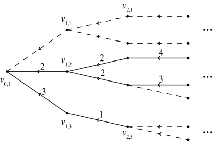
Figure 1. Example of a model tree $\Gamma$.

Orient the edges of $\Gamma$ toward $v_{0,1}$ and give $\Gamma$ the path length metric, with all edges assigned length $1$. We adopt the following convention for denoting vertices, edges, and labels.

• A symbol $v_{i,j}$ indicates a vertex at a distance $i$ from the root; vertices with initial index $i$ will be called the tier $i$ vertices.

• For each $v_{i,j}$, with $i>0$, $e_{i,j}$ denotes the unique oriented edge emanating from $v_{i,j}$ and $k_{i,j}=\mathcal{K}\left(e_{i,j}\right)$.

The null edges of $\Gamma$, together with their vertices, constitute a (possibly empty) subgraph $\Omega$ of $\Gamma$ where each component contains a unique vertex $v_{i,j}$ closest to $v_{0,1}$ in $\Gamma$. In this way, $\Omega$ may be viewed as a rooted forest (a disjoint union of rooted subtrees) $\left\{\Omega_{i,j}\right\}$, where an index $i,j$ indicates that $v_{i,j}$ is its root. Of course, not every vertex of $\Gamma$ is the root of a null subtree.

Two families of finite subtrees of $\Gamma$ also play a useful role: for each integer $i\geq 0$, let $\Gamma_{i}$ denote the $i$-neighborhood of $v_{0,1}$ in $\Gamma$ and $\Gamma_{i}^{+}=\Gamma_{i}\cap\Gamma^{+}$.

Remark 4.

The above definitions allow for the possibility $\Gamma=\left\{v_{0,1}\right\}$; but, except for that trivial case, $\Gamma$ must be infinite. In fact, every edge of $\Gamma$ is contained in some infinite edge path ray.

3.2. Model Base Spaces

Next we describe the model base space $X_{\Gamma}$ corresponding to a model graph $\Gamma$; it will contain $\Gamma$ as a subcomplex.

• Attach an oriented edge $e_{0,1}^{\prime}$ to $\Gamma$ by identifying each end to $v_{0,1}$; in a similar manner, attach an oriented edge $e_{i,j}^{\prime}$ at each $v_{i,j}$ for which $k_{i,j}\neq 0$. This completes the 1-skeleton of $X_{\Gamma}$. For later use, let $S_{i,j}^{1}$ denote the oriented circle in $X_{\Gamma}^{\left(1\right)}$ that is the image of $e_{i,j}^{\prime}$; it has natural base point $v_{i,j}$.

• For each $e_{i,j}$ with $k_{i,j}\neq 0$, attach a 2-cell $d_{i,j}$ to $X_{\Gamma}^{\left(1\right)}$ as follows: beginning with $\left[0,1\right]\times\left[0,1\right]$, identify the top and bottom faces with $e_{i,j}$, send the right face once around $e_{i,j}^{\prime}$, and the left face $k_{i,j}$ times around $e_{i-1,j^{\prime}}^{\prime}$, where $v_{i-1,j^{\prime}}$ is the terminal end of $e_{i,j}$. Notice that $d_{i,j}$ is the mapping cylinder of a canonical degree $k_{i,j}$ map of $S_{i,j}^{1}$ onto $S_{i-1,j^{\prime}}^{1}$. This completes the construction of $X_{\Gamma}$. See Figure 2.

  

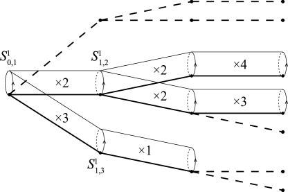
  Figure 2. Model base space $X_{\Gamma}$ corresponding to Figure 1.

  Denote by $X_{\Gamma^{+}}$ the subcomplex made up of $\Gamma^{+}$ together with all $e_{i,j}^{\prime}$ and all $d_{i,j}$; call $X_{\Gamma^{+}}$ the positive subcomplex of $X_{\Gamma}$. For each $i\geq 0$, let $X_{\Gamma_{i}}$ be the subcomplex of $X_{\Gamma}$ made up of $\Gamma_{i}$ and all $e_{i,j}^{\prime}$ and $d_{i,j}$ attached to $\Gamma_{i}$. Define $X_{\Gamma_{i}^{+}}$ similarly.

If we view the null edges of $\Gamma$ as mapping cylinders with singleton domains, then $X_{\Gamma}$ is made up entirely of mapping cylinders. In fact, if $W_{i}$ is the union of all $S_{i,j}^{1}$ and $v_{i,j}$ in the $i^{\text{th}}$ tier, and $\omega_{i}:W_{i}\rightarrow W_{i-1}$ be the union of maps taking the $S_{i,j}^{1}$ onto corresponding $S_{i-1,j^{\prime}}^{1}$ and $v_{i,j}$ to corresponding $v_{i-1,j^{\prime}}$, then $X_{\Gamma}$ is the inverse mapping telescope of the sequence

$$S_{0,1}^{1}=W_{0}\overset{\omega_{1}}{\longleftarrow}W_{1}\overset{\omega_{2}}{\longleftarrow}W_{2}\overset{\omega_{3}}{\longleftarrow}\cdots$$

The natural deformation retraction of $X_{\Gamma}$ onto $S_{0,1}^{1}$, which slides points along mapping telescope rays toward $S_{0,1}^{1}$, ends in a retraction $\rho:X_{\Gamma}\rightarrow S_{0,1}^{1}$. See [Gui16] for a discussion of inverse mapping telescopes.

For the next stage of our construction, it will be useful to have a thorough understanding of the point preimage $\rho^{-1}\left(v_{0,1}\right)$, which consists of all mapping telescope rays, both infinite and finite, emanating from $v_{0,1}$. (Finite mapping cylinder “rays” occur when an edge $e_{i,j}$ has label $k_{i,j}>1$ but all edges of $\Gamma$ with terminus $v_{i,j}$ are null.) By subdividing these rays in the obvious manner, with edges corresponding to the intersections with individual mapping cylinders and vertices corresponding to intersections with the $W_{i}$, $\rho^{-1}\left(v_{0,1}\right)$ becomes a tree $\Lambda$ with root vertex $v_{0,1}$. This tree contains $\Gamma$, but potentially much more. That is because each $d_{i,j}$, viewed as a mapping cylinder, contains $k_{i,j}$ distinct cylinder lines ending at base vertex $v_{i-1,j^{\prime}}$. Only one of those lines is an edge from $\Gamma$, but all are edges in $\Lambda$.

We now describe $\Lambda$ as the union of inductively defined subtrees $\Lambda_{1}\subseteq\Lambda_{2}\subseteq\cdots$.

Step 1. Beginning with $\Gamma_{1}$ as a building block, expand it to $\Lambda_{1}$ as follows. Replace each $e_{1,j}$ with label $k_{1,j}\neq 0$ with a wedge of $k_{1,j}$ inwardly oriented edges having common terminus $v_{0,1}$; color one edge from each such wedge black and the others gray. View the black edge as the “original” $e_{1,j}$ and its initial vertex as the original $v_{1,j}$; view the gray edges and their initial vertices as Step 1 “clones”. In addition, all null edges of $\Gamma_{1}$ are kept as edges of $\Lambda_{1}$. As before, they are indicated by a black dashed segment; the null edges do not get cloned. Call this finite tree, made up of all black, gray, and dashed edges and their vertices, $\Lambda_{1}$. The black and dashed edges form a copy of $\Gamma_{1}$ in $\Lambda_{1}$. The subtree $\Lambda_{1}^{+}$, made up of black and gray edges and their vertices, intersects $\Gamma_{1}$ in $\Gamma_{1}^{+}$. See Figure 3.

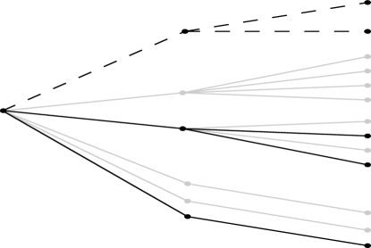
Figure 3. $\rho^{-1}\left(v_{0,1}\right)$ for the model base space in Figure 2.

Step 2. To construct $\Lambda_{2}$, attach additional edges and vertices to $\Lambda_{1}$ as follows. At the initial vertex $v_{1,j}$ of each edge of $\Gamma_{1}^{+}\leq\Lambda$ (the black edges), attach a wedge of $k_{2,j^{\prime}}$ edges for each non-null $e_{2,j^{\prime}}$ in $\Gamma_{2}$ terminating at $v_{1,j}$; color one edge from each wedge black and the others gray. View the black edge as the original $e_{2,j^{\prime}}$ and its initial vertex as $v_{2,j^{\prime}}$; the gray edges are Step 2 clones. In addition, at each clone of each $v_{1,j}$ (the gray edges of $\Lambda_{1}$), place a “wedge of wedges” identical to the one just attached at $v_{1,j}$, except that all of these edges are colored gray—they are also Step 2 clones. Finally, at the initial vertex $v_{1,j}$ of only the black and dashed edges of $\Lambda_{1}$ add an incoming dashed edge $e_{2,j^{\prime}}$ for each null $e_{2,j^{\prime}}$ in $\Gamma_{2}$ terminating at $v_{1,j}$. (As in Step 1, dashed edges do not get cloned.) Call the resulting finite graph $\Lambda_{2}$. The black and dashed edges, and their vertices form a copy of $\Gamma_{2}$ in $\Lambda_{2}$; meanwhile the black and gray edges form a subtree $\Lambda_{2}^{+}$ which intersects $\Gamma_{2}$ in $\Gamma_{2}^{+}$. Again see Figure 3.

Inductive steps. Continue the above process inductively outward to construct finite (colored trees) $\Lambda_{1}\subseteq\Lambda_{2}\subseteq\Lambda_{3}\subseteq\cdots$ whose union is the tree $\Lambda=\rho^{-1}\left(v_{0,1}\right)$, rooted at $v_{0,1}$ and containing $\Gamma$ as a rooted subtree (the black and dashed edges). The subtree consisting of all black and gray edges is denoted $\Lambda^{+}$; it intersects $\Gamma$ in $\Gamma^{+}$.

Remark 5.

Experts will notice a similarity between the above construction and a fundamental construction in Bass-Serre theory. At the conclusion of this section, we will make a concrete connection between the two.

3.3. Model $\mathbb{Z}$-spaces

We now look to understand model $\mathbb{Z}$-spaces $\widetilde{X}_{\Gamma}$, which are the universal covers of the $X_{\Gamma}$.

Let $q:\widetilde{X}_{\Gamma}\rightarrow X_{\Gamma}$ and $r:\mathbb{R}\rightarrow S_{0,1}^{1}$ be universal covering projections, where $S_{0,1}^{1}$ is viewed as the quotient of $\mathbb{Z}$ acting on $\mathbb{R}$ by unit translations. The lift $\widetilde{\rho}:\widetilde{X}_{\Gamma}\rightarrow\mathbb{R}$ of $\rho:X\rightarrow S_{0,1}^{1}$ will play a useful role as a “height function”. For example, in the case where $X_{\Gamma^{+}}\leq X_{\Gamma}$ is just $S_{0,1}^{1}$, $\widetilde{X}_{\Gamma}$ consists of a real line $\widetilde{S}_{0,1}^{1}$ taken homeomorphically onto $\mathbb{R}$ by $\widetilde{\rho}$, together with a copy of $\Lambda$ (in this case the same as $\Gamma$) attached at each integer height. The general case is similar, in that $\widetilde{X}_{\Gamma}$ is made up of $\widetilde{X}_{\Gamma^{+}}$ along with trees attached at integer heights; but now both $\widetilde{X}_{\Gamma^{+}}$ and the attachment pattern for the trees are more complicated. Since $X_{\Gamma^{+}}$ is built entirely from cylinders of nontrivial maps between circles, we can begin to understand $\widetilde{X}_{\Gamma^{+}}$ by looking at the universal cover of a single mapping cylinder.

The universal cover of the mapping cylinder $\mathcal{M}_{k}$ of a degree $k$ map $S^{1}\overset{\times k}{\longleftarrow}S^{1}$ can be realized as $\widetilde{\mathcal{M}}_{k}=\Lambda\left(k\right)\times\mathbb{R}$, where $\Lambda\left(k\right)$ is a wedge of arcs with common end point $a_{0}$ and distinct initial points $a_{1},\cdots,a_{k}$. Under the covering projection, the preimage of the range circle is the line $\{a_{0}\}\times\mathbb{R}$ and the preimage of the domain circle is $\left\{a_{1},\cdots,a_{k}\right\}\times\mathbb{R}$, one copy of $\mathbb{R}$ for each coset of $k\mathbb{Z}$ in $\mathbb{Z}$. The group of covering transformations is generated by the map $\sigma_{k}\times t$, where $\sigma_{k}:\Lambda\left(k\right)\rightarrow\Lambda\left(k\right)$ fixes $a_{0}$ and permutes the edges cyclically, and $t\left(r\right)=r+1$.

Working inductively outward from $S_{0,1}^{1}$, and replicating the above construction again and again, one sees that the subcomplex $\widetilde{X}_{\Gamma^{+}}$ may be identified with the product $\Lambda^{+}\times\mathbb{R}$, with the group of covering transformations being generated by a product map $\sigma_{\infty}\times t$, where $\sigma_{\infty}:\Lambda^{+}\rightarrow\Lambda^{+}$ is a homeomorphism that fixes $v_{0,1}$ and is determined by how it permutes the ends of $\Lambda^{+}$, and $t\left(r\right)=r+1$.

Remark 6.

The homeomorphism $\sigma_{\infty}:\Lambda^{+}\rightarrow\Lambda^{+}$ can be built inductively from the various $\sigma_{k}$ described above. A more algebraic description can be obtained from Bass-Serre theory, where $\Lambda^{+}$ is viewed as the Bass-Serre tree corresponding to a graph of groups interpretation of $\Gamma^{+}$ and $\sigma_{\infty}$ is the generator of the corresponding action. See §4.

In situations where $X_{\Gamma}=X_{\Gamma^{+}}$ (an important special case), the above provides a complete description of $\widetilde{X}_{\Gamma}$ as $\Lambda^{+}\times\mathbb{R}$ with covering transformations generated by $\sigma_{\infty}\times t$. In general, we must account for the portions of $\widetilde{X}_{\Gamma}$ lying over $X_{\Gamma}-X_{\Gamma^{+}}$. With respect to the height function, those portions lie entirely at integer levels, where $\widetilde{\rho}^{-1}\left(n\right)$ is a copy of $\Lambda$ intersecting $\Lambda^{+}\times\mathbb{R}$ in $\Lambda^{+}\times\{n\}$. At $n=0$, a copy of $\Lambda$ is glued to $\Lambda^{+}\times\mathbb{R}$ by identifying the subgraph $\Lambda^{+}$ with $\Lambda^{+}\times\{0\}$. For general height $n$, a copy of $\Lambda$ is attached along $\Lambda^{+}\times\{n\}$ by identifying $x\in\Lambda^{+}$ with $\,(\sigma_{\infty}^{n}\left(x\right),n)$.

To obtain a generator of the group of covering transformations on $\widetilde{X}_{\Gamma}$, we must extend $\sigma_{\infty}\times t$ over the copies of $\Lambda$ at the integral levels. Abusing notation slightly, $\widetilde{X}_{\Gamma}$ is the quotient of the disjoint union $(\Lambda^{+}\times\mathbb{R})\sqcup(\Lambda\times\mathbb{Z})$, where $\left(x,n\right)$ in the second summand is identified not with $\left(x,n\right)$ in the first, but rather, with $(\sigma_{\infty}^{n}\left(x\right),n)$ in the first summand. The generator of the covering transformations is obtained by gluing the maps $\sigma_{\infty}\times t:\Lambda^{+}\times\mathbb{R}\rightarrow\Lambda^{+}\times\mathbb{R}$ and $\operatorname*{id}\times t:\Lambda\times\mathbb{Z}\rightarrow\Lambda\times\mathbb{Z}$.

For easy reference, we assemble the key properties of $\widetilde{X}_{\Gamma}$ in a single proposition.

Proposition 3.1.

Let $\Gamma$ be a model tree, $X_{\Gamma}$ its model space, and $q:\widetilde{X}_{\Gamma}\rightarrow X_{\Gamma}$ the universal covering projection. Then $\widetilde{X}_{\Gamma}$ is a contractible 2-complex with $1,2$ or infinitely many ends. More specifically, the pair $\Gamma^{+}\leq\Gamma$ (together with their labelings) determine a pair of trees $\Lambda^{+}\leq\Lambda$, also rooted at $v_{0,1}$, with $\Gamma^{+}\leq\Lambda^{+}$ and $\Gamma\leq\Lambda$ such that:

1. $\widetilde{X}_{\Gamma}$ is $2$-ended if and only if $\Gamma=\Gamma^{+}=\left\{v_{0,1}\right\}$ (a single vertex). In that case $\Lambda=\Lambda^{+}=\left\{v_{0,1}\right\}$ and $\widetilde{X}_{\Gamma}\approx\mathbb{R}$, with the group of covering transformations generated by $t\left(r\right)=r+1$;

2. $\widetilde{X}_{\Gamma}$ is $1$-ended if and only if $\Gamma=\Gamma^{+}$ and the two are nontrivial (hence infinite). In that case $\Lambda=\Lambda^{+}$ and $\widetilde{X}_{\Gamma}\approx\Lambda^{+}\times\mathbb{R}$, with the corresponding group of covering transformations generated by a product of homeomorphisms $\sigma_{\infty}\times t:\Lambda^{+}\times\mathbb{R}\rightarrow\Lambda^{+}\times\mathbb{R}$, where $\sigma_{\infty}$ fixes the root of $\Lambda^{+}$ and $t\left(r\right)=r+1$;

3. $\widetilde{X}_{\Gamma}$ is infinite-ended if and only if $\Gamma^{+}\lneq\Gamma$. In that case $\Omega=\overline{\Gamma-\Gamma^{+}}$ is a nonempty forest $\left\{\Omega_{i,j}\right\}$ of infinite rooted trees, and $\widetilde{X}_{\Gamma}$ is homeomorphic to $\Lambda^{+}\times\mathbb{R}$ together with a $\mathbb{Z}$-equivariant family $\left\{n\Omega_{i,j}\right\}_{n\in\mathbb{Z}}$ of copies of each $\Omega_{i,j}$ attached to $\Lambda^{+}\times\mathbb{R}$ at their roots. More specifically, a generator of the covering transformations on $\widetilde{X}_{\Gamma}$ restricts to $\Lambda^{+}\times\mathbb{R}$ as a product of homeomorphisms $\sigma_{\infty}\times t:\Lambda^{+}\times\mathbb{R}\rightarrow\Lambda^{+}\times\mathbb{R}$, as described above, and $n\Omega_{i,j}$ is attached to $\Lambda^{+}\times\mathbb{R}$ by identifying its root to $\left(\sigma_{\infty}^{n}\left(v_{i,j}\right),n\right)$. The map $\sigma_{\infty}\times t$ extends to $\widetilde{X}_{\Gamma}$ in the obvious way.

Remark 7.

Case 3) of Proposition 3.1 can be split into subcases resembling the 2- and 1-ended situations, respectively.

Subcase a). When $\Gamma^{+}$ is finite, so is $\Lambda^{+}$, so a collapse of $\Lambda^{+}$ onto its root vertex induces an equivariant proper homotopy equivalence $f:\Gamma^{+}\times\mathbb{R}\rightarrow\mathbb{R}.$ If, at each integer $n$, we attach to $\mathbb{R}$ copies of the trees $n\Omega_{i,j}\subseteq\widetilde{X}_{\Gamma}$; then $f$ extends to an equivariant proper homotopy equivalence between $\widetilde{X}_{\Gamma}$ and the resulting locally finite graph comprised of $\mathbb{R}$ with trees attached at the integers.

Subcase b).When $\Gamma^{+}$ is infinite, there is no obvious simplification of $\widetilde{X}_{\Gamma}$, but an analogy with the 1-ended case remains. In particular $\widetilde{X}_{\Gamma}$ contains a large equivariant subcomplex identical to the 1-ended case, with the remainder of $\widetilde{X}_{\Gamma}$ consisting of a discrete collection of trees.

Under either of the two subcases, $\widetilde{X}_{\Gamma}$ has countably many ends, unless $\left\{\Omega_{i,j}\right\}$ contains a tree with uncountably many ends.

The usefulness of model spaces $X_{\Gamma}$ and $\widetilde{X}_{\Gamma}$ lies in the simplicity of their topology at infinity. Of particular interest here is their homotopy and homology data in dimensions 0 and 1.

Proposition 3.2.

Let $\Gamma$ be a model tree and $X_{\Gamma}$ the corresponding model space. Then the inclusion map $\Gamma\hookrightarrow X_{\Gamma}$ is a proper 1-equivalence, thereby inducing a bijection between ends. If $r$ is an edge path ray in $\Gamma$ beginning at $v_{0,1}$, then $\operatorname*{pro}$-$\pi_{1}\left(X_{\Gamma},r\right)$ can be represented by the inverse sequence

$$\mathbb{Z}\overset{\times k_{1,j_{1}}}{\longleftarrow}\mathbb{Z}\overset{\times k_{2,j_{2}}}{\longleftarrow}\mathbb{Z}\overset{\times k_{2,j_{3}}}{\longleftarrow}\cdots$$

where the $k_{i,j_{i}}$ are the labels on the edges that comprise $r$.

Of greater interest is the end behavior of the model $\mathbb{Z}$-spaces.

Proposition 3.3.

Let $\Gamma$ be a model tree, $X_{\Gamma}$ and $\widetilde{X}_{\Gamma}$ the corresponding model $\mathbb{Z}$-space. As noted in Proposition 3.1, $\widetilde{X}_{\Gamma}$ is 1-, 2-, or infinite-ended. Moreover,

1. If $\widetilde{X}_{\Gamma}$ is 2-ended, both ends are simply connected and the $\mathbb{Z}$-action fixes those ends;

2. If $\widetilde{X}_{\Gamma}$ is 1-ended, that end is semistable and $\operatorname*{pro}$-$\pi_{1}\left(\widetilde{X}_{\Gamma},r\right)$ can be represented by an inverse sequence of surjections between finitely generated free groups

   $$F_{1}\twoheadleftarrow F_{2}\twoheadleftarrow F_{3}\twoheadleftarrow\cdots$$

   and $\operatorname*{pro}$-$H_{1}\left(\widetilde{X}_{\Gamma};\mathbb{Z}\right)$ can be represented by an inverse sequence of surjections between finitely generated free abelian groups

   $$\mathbb{Z}^{n_{1}}\twoheadleftarrow\mathbb{Z}^{n_{2}}\twoheadleftarrow\mathbb{Z}^{n_{3}}\twoheadleftarrow\cdots.$$

3. If $\widetilde{X}_{\Gamma}$ is infinite-ended, the $\mathbb{Z}$-action fixes precisely one or two ends with the others having trivial stabilizers. All non-fixed ends are simply-connected. If two ends are fixed, those ends are simply connected as well. If just one end is fixed, that end is semistable with $\operatorname*{pro}$-$\pi_{1}\left(\widetilde{X}_{\Gamma},r\right)$ representable by an inverse sequence like the one described in Assertion (2). Similarly, $\operatorname*{pro}$-$H_{1}\left(\widetilde{X}_{\Gamma};\mathbb{Z}\right)$ is representable by a sequence like the one found in Assertion (2), with all nontrivial contributions coming from the fixed end.

Proof.

The only assertions not immediate from Proposition 3.1 are the representations of $\operatorname*{pro}$-$\pi_{1}\left(\widetilde{X}_{\Gamma},r\right)$ and $\operatorname*{pro}$-$H_{1}\left(\widetilde{X}_{\Gamma};\mathbb{Z}\right)$. Let us first address the 1-ended case where, by Proposition 3.1, $\widetilde{X}_{\Gamma}$ may be identified with $\Lambda^{+}\times\mathbb{R}$, with $\Lambda^{+}$ an infinite leafless tree rooted at $v_{0,1}$. Let $r=$ $v_{0,1}\times[0,\infty)$ be the base ray, and $N_{1}\supseteq N_{2}\supseteq\cdots$ the cofinal sequence of neighborhoods of infinity, where $N_{i}=\Lambda^{+}\times\mathbb{R}-[\mathring{\Lambda}_{i}^{+}\times\left(-i,i\right)]$. Here $\mathring{\Lambda}_{i}^{+}$ is the open $i$-ball in $\Lambda_{i}$ centered at $v_{0,1}$. It is easy to see that $N_{i}$ deformation retracts onto its frontier in $\Lambda^{+}\times\mathbb{R}$,

$$\operatorname*{Fr}\nolimits_{\Lambda^{+}\times\mathbb{R}}N_{i}=\Lambda_{i}^{+}\times\left\{-i,i\right\}\cup(\operatorname*{Fr}\nolimits_{\Lambda^{+}}\Lambda_{i}^{+}\times\left[-i,i\right])$$

where $\operatorname*{Fr}_{\Lambda^{+}}\Lambda_{i}^{+}$ is the set of vertices in $\Lambda^{+}$ at a distance $i$ from $v_{0,1}$. By squeezing $\Lambda_{i}^{+}\times\left\{-i\right\}$ and $\Lambda_{i}^{+}\times\left\{i\right\}$ to points, $\operatorname*{Fr}\nolimits_{\Lambda^{+}\times\mathbb{R}}N_{i}$ is seen to be homotopy equivalent to the suspension of $\operatorname*{Fr}_{\Lambda^{+}}\Lambda_{i}^{+}$, a space whose fundamental group is free of rank $\left|\operatorname*{Fr}_{\Lambda^{+}}\Lambda_{i}^{+}\right|-1$; call that group $F_{i}$. To complete Assertion (2), it remains to show that bonding maps $F_{i}\longleftarrow F_{i+1}$ are surjective. Since $\Lambda^{+}$ has no leaves, the collapse of $\Lambda_{i+1}^{+}$ onto $\Lambda_{i}^{+}$ restricts to a surjection of $\operatorname*{Fr}\nolimits_{\Lambda^{+}}\Lambda_{i+1}^{+}$ onto $\operatorname*{Fr}\nolimits_{\Lambda^{+}}\Lambda_{i}^{+}$, which can be suspended to get a map making the following diagram commute up to homotopy.

$$N_{i}$$

          

Surjectivity of the induced maps on fundamental groups is now clear.

To obtain an equivalent representation of $\operatorname*{pro}$-$\pi_{1}\left(\widetilde{X}_{\Gamma},r\right)$ in the infinite-ended case with a single fixed end, note that the fixed end can be represented by a sequence $M_{1}\supseteq M_{2}\supseteq\cdots$ of components of neighborhoods of infinity where each $M_{i}$ is homeomorphic to an $N_{i}$ from the previous case, with a countable collection of locally finite trees attached at a discrete collection of points. Since $M_{i}$ deformation retracts onto $N_{i}$, the above calculations are still valid.

The proposed representations of $\operatorname*{pro}$-$H_{1}\left(\widetilde{X}_{\Gamma};\mathbb{Z}\right)$ follow easily. ∎

Remark 8.

If desired, more detail on the representations of $\operatorname*{pro}$-$\pi_{1}\left(\widetilde{X}_{\Gamma},r\right)$ and $\operatorname*{pro}$-$H_{1}\left(\widetilde{X}_{\Gamma};\mathbb{Z}\right)$ can be obtained; for example, formulas for the bonding maps, and a description of the induced $\mathbb{Z}$-action on the inverse sequences can be deduced from the above analysis.

3.4. Reductions of model spaces

We close this section by describing a “reduction” procedure that can be applied to a model tree and passed along to its resulting model spaces. Beginning with a model tree $\Gamma$ and a pair of integers $0\leq i<j$, the elementary $[i,j]$-reduction is accomplished by removing all edges in $\overline{\Gamma_{j}-\Gamma_{i}}$, then putting in a single edge from each tier $j$ vertex $v_{j,r}$ to the unique tier $i$ vertex $v_{i,s}$ on the reduced edge path connecting $v_{j,r}$ to the root vertex $v_{0,1}$. The label on that new edge is the product of the labels on the edge path in $\Gamma$ connecting $v_{j,r}$ to $v_{i,s}$. If the new tree is denoted $\Gamma^{\prime}$ then, topologically, $\Gamma^{\prime}$ is obtained from $\Gamma$ by crushing each component of $\overline{\Gamma_{j-1}-\Gamma_{i}}$ to a point.

The difference between $X_{\Gamma}$ and $X_{\Gamma^{\prime}}$ is easy to discern. Remove from $X_{\Gamma}$ the interior of $\overline{X_{\Gamma_{j}}-X_{\Gamma_{i}}}$; then, for each tier $j$ circle $S_{j,r}^{1}$ replace the “path of mapping cylinders” in $X_{\Gamma}$ from $S_{j,r}^{1}$ to $S_{i,s}^{1}$ with a single mapping cylinder whose map is the composition of the maps along that path. For a “naked” tier $j$ vertex, simply insert a naked edge connecting it to the corresponding tier $i$ vertex. A standard fact about mapping cylinders is that, for a composition $A\overset{f}{\longrightarrow}B\overset{g}{\longrightarrow}C$, the mapping cylinder $\operatorname*{Map}\left(gf\right)$ of the composition is homotopy equivalent rel $A\cup C$ to the union $\operatorname*{Map}\left(f\right)\cup_{B}\operatorname*{Map}\left(g\right)$ of mapping cylinders. Applying this fact repeatedly, one obtain a proper homotopy equivalence, fixed outside the interior of $\overline{X_{\Gamma_{j}}-X_{\Gamma_{i}}}$, between $X_{\Gamma}$ and $X_{\Gamma^{\prime}}$.

A reduction of $\Gamma$ is obtained by performing the above procedure over a, possibly infinite, sequence of closed intervals $\left\{\left[i_{k},j_{k}\right]\right\}$ with $j_{k}\leq i_{k+1}$ for all $k$. By applying the above procedure repeatedly, and then lifting to universal covers, we obtain the following useful fact.

Proposition 3.4.

Let $\Gamma^{\prime}$ be a model tree obtained by reduction of a model tree $\Gamma$. Then the model base spaces $X_{\Gamma^{\prime}}$ and $X_{\Gamma}$ are proper homotopy equivalent and the model $\mathbb{Z}$-spaces $\widetilde{X}_{\Gamma^{\prime}}$ and $\widetilde{X}_{\Gamma}$ are equivariantly proper homotopy equivalent.

Example 9.

The proper homotopy equivalence discussed in subcase a) of Remark 7 can now be viewed as the result of a reduction. Choose $j$ so large that $\Gamma^{+}\subseteq\Gamma_{j}$ and perform the elementary $[i,j]$-reduction.

4. Connections to Bass-Serre theory

This section is a brief diversion. Bass-Serre theory is not needed for the purposes of this paper, but for those with a previous understanding of that topic, the connection can make some of our constructions easier to follow.

Beginning with a model tree $\Gamma$, create a graph of groups as follows: place a copy of $\mathbb{Z}$ on each vertex and each edge of $\Gamma^{+}$ and a trivial group $0$ on the vertices and edges in $\Gamma-\Gamma^{+}$; then interpret the labels $k_{i,j}$ as multiplication homomorphisms. The result is an elaborate graph of groups decomposition of $\mathbb{Z}$, where the copy of $\mathbb{Z}$ at the root vertex includes isomorphically into the fundamental group of the graph of groups. (All homomorphisms on reversed edges are identities.) The model space $X_{\Gamma}$ is the corresponding total space for $\Gamma$, as described in [SW79] and [Geo08, Ch.6]. The subgraph $\Gamma^{+}$ determines a simpler graph of groups decomposition of $\mathbb{Z}$ that is consistent with $\Gamma$ and has total space $X_{\Gamma}^{+}\subseteq X_{\Gamma}$. The tree $\Lambda^{+}$ constructed above is the Bass-Serre tree corresponding to $\Gamma^{+}$ and $\sigma_{\infty}$ is a generator of the corresponding action. See [Ser80, Ch.I, §4.5].

The Bass-Serre tree $\Lambda^{\ast}$ for the full graph of groups $\Gamma$ does not play a direct role here, but it is lurking in the background. One may expand $\Lambda$ to $\Lambda^{\ast}$ as follows: Viewing $\Gamma$ as a subset of $\Lambda$, replace each subtree $\Omega_{i,j}\leq\Gamma$ with a countably infinite wedge of copies of $\Omega_{i,j}$, all joined at the root vertex $v_{i,j}$ of $\Omega_{i,j}$. Designate one copy as the original $\Omega_{i,j}$ and the rest as clones. Then, at each clone of $v_{i,j}$ in $\Lambda$, attach another infinite wedge of copies of $\Omega_{i,j}$, all viewed as clones. The need for countably infinite collections is because the group at $v_{i,j}$ is $\mathbb{Z}$ while all incoming edge groups are trivial, and thus have countably infinite index in the vertex group at $v_{i,j}$.

5. Associating models to $\mathbb{Z}$-actions

We return to the primary objects of interest—simply connected, locally compact ANRs admitting $\mathbb{Z}$-actions by covering transformations. Observations from Sections 1.4 and 2 allow us to focus on strongly locally finite CW complexes (or even locally finite polyhedra) admitting such $\mathbb{Z}$-actions. In this section, we prove the primary technical results of this paper. At the conclusion, we will have obtained the following:

Theorem 5.1.

For $Y$ a simply connected, locally compact ANR, and $j:Y\rightarrow Y$ a homeomorphism generating an action by covering transformations with $J\equiv\left\langle j\right\rangle\cong\mathbb{Z}$, there is a corresponding model tree $\Gamma$ so that

1. $\widetilde{X}_{\Gamma}$ is $\mathbb{Z}$–equivariantly properly $1$-equivalent to $Y$,

2. If $j$ is strongly coaxial, $J\backslash Y$ is properly 2-equivalent to $X_{\Gamma}$; hence $Y$ is $\mathbb{Z}$-equivariantly properly 2-equivalent to $\widetilde{X}_{\Gamma}$.

3. If $j$ is coaxial, $Y$ is properly 2-equivalent to $\widetilde{X}_{\Gamma}$ via proper 2-equivalences that are $\mathbb{Z}$-equivariant on 1-skeleta.

By our work in Sections 1.4 and 2, it is enough to consider the case where $Y$ is a simply connected, strongly locally finite CW complex, and $j:Y\rightarrow Y$ is a cellular homeomorphism generating an action by covering transformations with $J\equiv\left\langle j\right\rangle\cong\mathbb{Z}$. Our first goal is to associate a model tree $\Gamma$ to this action. Begin by choosing a nested cofinal sequence $J\backslash Y=N_{0}\supseteq N_{1}\supseteq N_{2}\supseteq\cdots$ of subcomplex neighborhoods of infinity in $J\backslash Y$. By discarding compact components, we may assume that each of the (finitely many) components $\left\{N_{i,j}\right\}_{j=1}^{r_{i}}$ of each $N_{i}$ is unbounded.

Choose an oriented edge path loop $\alpha_{0,1}$ in $N_{0}=J\backslash Y$ that generates $H_{1}\left(J\backslash Y\right)\cong\mathbb{Z}$. For each component $N_{i,j}$ of each $N_{i}$ consider the inclusion induced map $H_{1}(J\backslash Y)\overset{i_{\ast}}{\longleftarrow}H_{1}\left(N_{i,j}\right)$. (All homology is with $\mathbb{Z}$-coefficients.) If the map is nontrivial, let $n_{i,j}$ be the index of $i_{\ast}\left(H_{1}\left(N_{i,j}\right)\right)$ in $H_{1}(J\backslash Y)$, and choose an oriented edge path loop $\alpha_{i,j}$ in $N_{i,j}$ taken to $n_{i,j}\alpha_{0,1}$ by $i_{\ast}$; if it is trivial, let $n_{i,j}=0$ and let $\alpha_{i,j}$ be a constant edge path loop in $N_{i,j}$.

Remark 9.

Use of homology rather than fundamental group, in defining $n_{i,j}$ and $\alpha_{i,j}$, allows us to avoid base point technicalities without loss of any essential information.

Let $K_{0}$ be a finite connected subcomplex of $J\backslash Y$ that contains $\alpha_{0,1}$, and for each $i>0$, let $K_{i}$ be a finite connected subcomplex of $J\backslash Y$ chosen sufficiently large so that

1. $\overline{J\backslash Y-N_{i}}\subseteq K_{i}$,

2. for every pair of vertices in the frontier of a component $N_{i,j}$ of $N_{i}$, $K_{i}$ contains an edge path in $N_{i,j}$ connecting them, and

3. $K_{i}$ contains each loop in the collection $\left\{\alpha_{i,j}\right\}_{j=1}^{r_{i}}$.

By passing to a subsequence and relabeling, we may assume that $N_{i+1}\subseteq J\backslash Y-K_{i}$ for all $i$. Let $L_{i}=N_{i}\cap K_{i}$ and $M_{i}=N_{i}\cap K_{i+1}$; then $M_{i}$ is a finite complex containing disjoint subcomplexes $L_{i}$ and $L_{i+1}$, and $M_{i}\cap M_{i+1}=L_{i+1}$. For each component $N_{i,j}$ of $N_{i}$, let $L_{i,j}=N_{i,j}\cap L_{i}$ and $M_{i,j}=N_{i,j}\cap M_{i}$. By connectedness of $K_{i}$ and $N_{i,j}$, along with property 2, each $L_{i,j}$ and $M_{i,j}$ is connected; moreover, $M_{i,j}$ contains a component $L_{i+1,k}$ of $L_{i+1}$ if and only if $N_{i,j}$ contains $N_{i+1,k}$. See Figure 4.

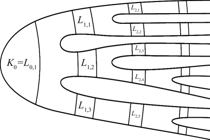
Figure 4. Decomposition of $J\backslash Y$ into subcomplexes.

Let $\Gamma$ be the rooted tree with a vertex $v_{i,j}$ for each $L_{i,j}$ and an edge between $v_{i,p}$ and $v_{i+1,q}$ whenever $L_{i+1,q}\subseteq M_{i,p}$ (equivalently $N_{i+1,q}\subseteq N_{i,p}$). The root vertex $v_{0,1}$ corresponds to the single component $L_{0,1}$ of $L_{0}=K_{0}$ lying in $N_{0,1}=N_{0}=J\backslash Y$. Since the $N_{i}$ have no compact components, $\Gamma$ has no valence $1$ vertices.

Orient the edges of $\Gamma$ in the direction of $v_{0,1}$ and for each $v_{i,j}$ with $i>0$, let $e_{i,j}$ denote the unique oriented edge emanating from $v_{i,j}$. Label each $e_{i,j}$ with an integer $k_{i,j}$ as follows. For the edges $e_{1,j}$ terminating at the root, let $k_{1,j}=n_{1,j}$. For $i>1$, $k_{i,j}=0$ if $n_{i,j}=0$; otherwise let $k_{i,j}=\frac{n_{i,j}}{n_{i-1,j^{\prime}}}$, where $N_{i-1,j^{\prime}}$ is the unique component of $N_{i-1}$ containing $N_{i,j}$. Since the map $H_{1}(J\backslash Y)\overset{i_{\ast}}{\longleftarrow}H_{1}\left(N_{i,j}\right)$ used to define $n_{i,j}$ factors through $H_{1}\left(N_{i-1,j^{\prime}}\right)$, $k_{i,j}$ is an integer; moreover, for any $v_{i,j}$ the integer $n_{i,j}$ can be recovered by multiplying the labels on the edge path connecting $v_{i,j}$ to $v_{0,1}$. Note that $\Gamma$ satisfies all conditions laid out in §3 for a model tree; therefore, all definitions, notation, and subsequent constructions from that section can be carried forward.

The tree $\Gamma$ is a good model for $\mathcal{E}\emph{nds}\left(J\backslash Y\right)$. Indeed, repeated application of the Tietze extension theorem produces a proper 1-equivalence from $J\backslash Y$ to $\Gamma$. Unfortunately, that map is of limited use: first, it has no chance of providing information about higher-dimensional end invariants; and second, it tells us nothing about the space $Y$, which is our primary interest. To address those problems we construct a more delicate, map $f:J\backslash Y\rightarrow X_{\Gamma}$ which incorporates some higher-dimensional information and lifts to a map $\widetilde{f}:Y\rightarrow\widetilde{X}_{\Gamma}$.

Let $r:X_{\Gamma}\rightarrow\Gamma$ be the retraction sending each circle $S_{i,j}^{1}$ onto $v_{i,j}$, and more generally, squashes each mapping cylinder $d_{i,j}$ onto $e_{i,j}$ in a level-preserving manner, with point preimages being circles. Notice that $r^{-1}\left(\Gamma^{+}\right)=X_{\Gamma^{+}}$. For each $i$, let $X_{\Gamma_{i}}=r^{-1}\left(\Gamma_{i}\right)$ and $Q_{i}=\overline{X_{\Gamma}-X_{\Gamma_{i}}}$. Then $X_{\Gamma_{0}}\subseteq X_{\Gamma_{1}}\subseteq X_{\Gamma_{2}}\subseteq\cdots$ is a filtration of $X_{\Gamma}$ by finite subcomplexes, and $X_{\Gamma}=Q_{0}\supseteq Q_{1}\supseteq Q_{2}\supseteq\cdots$ is a cofinal sequence of subcomplex neighborhoods of infinity. For each $i$, let $P_{i}=Q_{i}\cap X_{\Gamma_{i+1}}=r^{-1}\left(\overline{\Gamma_{i+1}-\Gamma_{i}}\right)$, a finite subcomplex consisting of $\overline{\Gamma_{i+1}-\Gamma_{i}}$ with mapping cylinders attached along the non-null edges.

By construction, there is a one-to-one correspondence between the sequences of neighborhoods of infinity $\left\{N_{i}\right\}$ and $\left\{Q_{i}\right\}$ so that the components $\left\{N_{i,j}\right\}$ of $N_{i}$ are in one-to-one correspondence with the components $\left\{Q_{i,j}\right\}$ of $Q_{i}$. Moreover, for each component $M_{i,j}$ of $M_{i}$, which contains a connected subcomplex $L_{i,j}$ on its “left-hand side” and a disjoint collection of similar subcomplexes $\{L_{i+1,j^{\prime}}\}$ on its “right-hand side”, the corresponding component $P_{i,j}$ of $P_{i}$ has a left-hand side consisting of a circle $S_{i,j}^{1}$ or vertex $v_{i,j}$ and a right-hand side made up of circles and vertices, labeled $S_{i+1,j^{\prime}}^{1}$ or $v_{i+1,j^{\prime}}$ (one for each subcomplex $L_{i+1,j^{\prime}}$ in $M_{i,j}$). If some of right-hand components of $P_{i,j}$ are circles, the left-hand side must be a circle, and $P_{i,j}$ is made up of a union of mapping cylinders of degree $k_{i+1,j^{\prime}}$ maps $S_{i,j}^{1}\leftarrow S_{i+1,j^{\prime}\text{ }}^{1}$ (one for each right-hand circle) intersecting in a common range circle and “naked edges” connecting the isolated vertices of the right-hand side to $v_{i,j}$ on the left-hand side. The map $f:J\backslash Y\rightarrow X$ will be most easily understood from its restrictions $f_{i,j}:M_{i,j}\rightarrow P_{i,j}$. See Figure 5.

Figure 5. A building block of $f:J\backslash Y\rightarrow X_{\Gamma}$.

Choose a maximal tree $T_{i,j}$ in each $L_{i,j}$ then choose a maximal tree $T_{i,j}^{{}^{\prime}}$ in each $M_{i,j}$ containing both $T_{i,j}$ and all $T_{i+1,j^{\prime}}$ contained in $M_{i,j}$. Let $T=\cup T_{i,j}^{{}^{\prime}}$. The tree-like structure of the collection $\left\{M_{i,j}\right\}$ ensures that $T$ a maximal tree in $J\backslash Y$. Select a base vertex $p_{i,j}$ from each $L_{i,j}$, making sure that $p_{i,j}$ lies on the edge loop $\alpha_{i,j}\subseteq L_{i,j}$ chosen previously. For each $L_{i+1,j^{\prime}}$ on the right-hand side of an $M_{i,j}$, let $\lambda_{i+1,j^{\prime}}$ be the unique edge path in $T_{i,j}^{\prime}$ from $p_{i,j}$ to $p_{i+1,j^{\prime}}$.

Define $f:T\rightarrow X_{\Gamma}$ by sending each $T_{i,j}$ to $v_{i,j}$ and every vertex of a $T_{i,j}^{\prime}$ not lying in one of those subtrees to $v_{i,j}$. For each remaining edge $e$ of $T$, choose the $T_{i,j}^{\prime}$ containing it. If both ends of $e$ have been sent to $v_{i,j}$, send $e$ to $v_{i,j}$; if one end has been sent to $v_{i,j}$ and the other to a $v_{i+1,j^{\prime}}$, map $e$ homeomorphically onto $e_{i+1,j^{\prime}}$; if one end lies in a $T_{i+1,j^{\prime}}$ and the other in a different $T_{i+1,j^{\prime\prime}}$, send the midpoint of $e$ to $v_{i,j}$ and the two halves of $e$ onto $e_{i+1,j^{\prime}}$ and $e_{i,j^{\prime\prime}}$, respectively.

Next we extend $f$ over the $L_{i,j}$. Each $L_{i,j}$ will be mapped into the circle $S_{i,j}^{1}$, when that circle exists, otherwise to the vertex $v_{i,j}$. Begin with $L_{0,1}=K_{0}$, which contains an oriented edge path loop $\alpha_{0,1}$ that generates $H_{1}\left(J\backslash Y\right)$. Let $\phi_{0,1}:H_{1}\left(J\backslash Y\right)\rightarrow\pi_{1}\left(S_{0,1}^{1},v_{0,1}\right)$ be the isomorphism taking $\alpha_{0,1}$ to the positively oriented generator of $\pi_{1}\left(S_{0,1},v_{0,1}\right)$, and consider the composition

$$\pi_{1}\left(L_{0,1},p_{0,1}\right)\twoheadrightarrow H_{1}\left(L_{0,1}\right)\twoheadrightarrow H_{1}\left(J\backslash Y\right)\overset{\phi_{0,1}}{\longrightarrow}\pi_{1}\left(S_{0,1}^{1},v_{0,1}\right)\text{.}$$

Recalling that $f$ has already been defined to send $T_{0,1}$ to $v_{0,1}$, we extend over the remaining edges of $L_{0,1}$. If $e$ is one such edge then, by giving it an orientation, it may be viewed as an element of $\pi_{1}\left(L_{0,1},p_{0,1}\right)$ and mapped into $S_{0,1}^{1}$ in accordance with its image under the above homomorphism. Having mapped the 1-skeleton of $L_{0,1}$ into $S_{0,1}^{1}$ in accordance with a $\pi_{1}$-homomorphism, we may extend to the 2-skeleton of $L_{0,1}$; then, by the asphericity of $S_{0,1}^{1}$, we may extend to all of $L_{0,1}$. See, for example, [Geo08, §7.1].

For general $L_{i,j}$, if $n_{i,j}=0$, send all of $L_{i,j}$ to $v_{i,j}$; otherwise, the argument used above is repeated to map $L_{i,j}$ into $S_{i,j}^{1}$, except that the map is based on the homomorphism

(5.1) $$\pi_{1}\left(L_{i,j},p_{i,j}\right)\twoheadrightarrow H_{1}\left(L_{i,j}\right)\twoheadrightarrow n_{i,j}\left\langle\alpha_{0,1}\right\rangle\overset{\phi_{i,j}}{\longrightarrow}\pi_{1}\left(S_{i,j}^{1},v_{i,j}\right)$$

where $n_{i,j}\left\langle\alpha_{0,1}\right\rangle\leq H_{1}\left(J\backslash Y\right)$ and $\phi_{i,j}$ is the (purely algebraic) isomorphism taking the generator $n_{i,j}\alpha_{0,1}$ to the oriented generator of $\pi_{1}\left(S_{i,j}^{1},v_{i,j}\right)$.

In the final step, we extend $f$ to all of $J\backslash Y$ by building maps $f_{i,j}:M_{i,j}\rightarrow P_{i,j}$ that agree on their overlaps. In the trivial cases, where $P_{i,j}$ is a wedge of of arcs, the existing map extends to $M_{i,j}$ by the Tietze extension theorem. In the nontrivial cases, $P_{i,j}$ strong deformation retracts onto $S_{i,j}^{1}$, and under that retraction each $S_{i+1,j^{\prime}}^{1}$ is wrapped $k_{i+1,j^{\prime}}$ times around $S_{i,j}^{1}$. Since $P_{i,j}$ is aspherical, we can use nearly the same strategy as above, based on an analogous homomorphism

$$\pi_{1}\left(M_{i,j},p_{i,j}\right)\twoheadrightarrow H_{1}\left(M_{i,j}\right)\twoheadrightarrow n_{i,j}\left\langle\alpha_{0,1}\right\rangle\overset{\psi_{i,j}}{\longrightarrow}\pi_{1}\left(P_{i,j},v_{i,j}\right)$$

On the subcomplex $T_{i,j}^{\prime}\cup L_{i,j}\cup\left(\cup L_{i+1,j^{\prime}}\right)$ of $M_{i,j}$, where $f$ has already been defined, the induced map into $\pi_{1}\left(P_{i,j},v_{i,j}\right)$ agrees with the target homomorphism, so we may extend to the remaining edges, as dictated by the homomorphism, and then to the remaining 2-cells, whose boundaries have been sent to trivial loops in $P_{i,j}$. Finally, asphericity of $P_{i,j}$ allows us to inductively extend over the remaining cells of $M_{i,j}$.

Proposition 5.2.

The map $f:J\backslash Y\rightarrow X_{\Gamma}$ is a proper 1-equivalence.

Proof.

Since $\left\{X_{\Gamma_{i}}\right\}$ is a finite filtration of $X_{\Gamma}$ and $f^{-1}\left(X_{\Gamma_{i}}\right)=K_{i}$ for each $i$, $f$ is proper. To complete the proof, we construct a proper map $g^{\left(1\right)}:X_{\Gamma}^{\left(1\right)}\rightarrow J\backslash Y$ such that $\left.gf\right|_{J\backslash Y^{\left(0\right)}}$ is properly homotopic to $J\backslash Y^{\left(0\right)}\hookrightarrow J\backslash Y$ and $\left.fg\right|_{X^{\left(0\right)}}$ is properly homotopic to $X_{\Gamma}^{\left(0\right)}\hookrightarrow X_{\Gamma}$.

For each $v_{i,j}\in X_{\Gamma}^{\left(0\right)}$, let $g\left(v_{i,j}\right)=p_{i,j}$. Map each $e_{i,j}$ originating at $v_{i,j}$ and ending at $v_{i-1,j^{\prime}}$ homeomorphically onto the (reversed) edge path $\lambda_{i,j}$ between $p_{i,j}$ and $p_{i-1,j^{\prime}}$ in $T_{i-1,l^{j\prime}}^{\prime}$; and map each oriented $e_{i,j}^{\prime}$ once around the oriented edge path loop $\alpha_{i,j}$ beginning and ending at $p_{i,j}$.

Since $g^{\left(1\right)}\left(P_{i,j}^{\left(1\right)}\right)\subseteq M_{i,j}$, then $g^{\left(1\right)}\left(Q_{i}^{\left(1\right)}\right)\subseteq N_{i}$ for all $i$; so $g^{\left(1\right)}$ is proper. Notice that $\left.fg^{\left(1\right)}\right|_{X^{\left(0\right)}}=\operatorname*{id}_{X^{\left(0\right)}}$ and, for each vertex $p\in J\backslash Y$, if $p\in M_{i,j}$, then $f\left(p\right)\in P_{i,j}$; so $g^{\left(1\right)}\left(f\left(p\right)\right)\in M_{i,j}$. A choice of edge path $\mu_{p}$ in $M_{i,j}$ from $p$ to $g^{\left(1\right)}\left(f\left(p\right)\right)$ for each $p\in M_{i,j}$ determines a proper homotopy between the inclusion and $\left.g^{\left(1\right)}f\right|_{J\backslash Y^{\left(0\right)}}$. ∎

Remark 10.

The above construction accomplishes more than required for a 1-equivalence; specifically, $fg^{\left(1\right)}$ is properly homotopic to $X_{\Gamma}^{\left(1\right)}\hookrightarrow X_{\Gamma}$. To see this, note that each oriented edge $e_{i,j}$ from $v_{i,j}$ to $v_{i-1,j^{\prime}}$ is mapped by $g^{\left(1\right)}$ to the edge path $\lambda_{i,j}$ from $p_{i,j}$ to $p_{i-1,j^{\prime}}$ and $f$ sends $\lambda_{i,j}$ entirely into $e_{i,j}$ with $f\left(p_{i,j}\right)=v_{i,j}$ and $f\left(p_{i-1,j^{\prime}}\right)=v_{i-1,j^{\prime}}$. A discrete collection of straightening homotopies, each supported in an edge $e_{i,j}$ and fixing all vertices, combine to properly homotope $fg^{\left(1\right)}$ to the identity over the tree $\Gamma$. For the “loop edges” $e_{i,j}^{\prime}$, the story is similar. The map $g^{\left(1\right)}$ takes $e_{i,j}^{\prime}$ once around $\alpha_{i,j}\subseteq L_{i,j}$ and $f$ returns $\alpha_{i,j}$ (in fact, all of $L_{i,j}$) to $S_{i,j}^{1}=e_{i,j}^{\prime}\cup v_{i,j}$, with vertices going to $v_{i,j}$, some edges sent entirely to $v_{i,j}$ and others around $S_{i,j}^{1}$ (possibly multiple times, in the forward or reverse directions). Since homomorphism 5.1, used to define $f$ on $L_{i,j}$, takes $\alpha_{i,j}$ to the positively oriented generator of $\pi_{1}\left(S_{i,j}^{1},v_{i,j}\right)$, $\left.fg^{\left(1\right)}\right|_{e_{i,j}^{\prime}}$ is homotopic to the identity by a base point preserving homotopy supported in $e_{i,j}$. A discrete collection of such homotopies completes the straightening process.

The proper 1-inverse $g^{\left(1\right)}:X_{\Gamma}^{\left(1\right)}\rightarrow J\backslash Y$ of $f:J\backslash Y\rightarrow X_{\Gamma}$ becomes more useful when extended to all of $X_{\Gamma}$, even if that extension is not proper. With the aid of a “strongly coaxial” hypothesis, a proper extension becomes possible.

Proposition 5.3.

The map $g^{\left(1\right)}:X_{\Gamma}^{\left(1\right)}\rightarrow J\backslash Y$ constructed in the proof of Proposition 5.2 can always be extended to a map $g:X_{\Gamma}\rightarrow J\backslash Y$ that induces a $\pi_{1}$-isomorphism. If $j$ is strongly coaxial, $g$ can be chosen to be a proper 2-inverse for $f$.

Proof.

To obtain $g:X_{\Gamma}\rightarrow J\backslash Y$, we need only extend $g^{\left(1\right)}$ over the 2-cells $d_{i,j}$ of $X_{\Gamma}$. Each $d_{i,j}$ is glued to $X_{\Gamma}^{\left(1\right)}$ along a loop of the form $(e_{i,j}^{\prime})^{k_{i,j}}\cdot e_{i,j}\cdot(e_{i-1,j^{\prime}}^{\prime})^{-1}\cdot(e_{i,j})^{-1}$, and that loop is mapped to $(\alpha_{i,j})^{k_{i,j}}\cdot\lambda_{i,j}\cdot(\alpha_{i-1,j^{\prime}})^{-1}\cdot(\lambda_{i,j})^{-1}$ which is homologically, and hence homotopically, trivial in $J\backslash Y$. So the map can be extended.

If $j$ is strongly coaxial, then by Lemma 2.8, we may (by passing to a subsequence of $\left\{K_{i}\right\}$) assume that, for each $n\geq 1$, loops in $J\backslash Y-K_{n}$ that are null-homotopic in $J\backslash Y$ contract in $J\backslash Y-K_{n-1}$. Since the attaching loop for each $d_{i,j}$, lies in $P_{i}\subseteq X_{\Gamma}-X_{\Gamma_{i-1}}$, its image $(\alpha_{i,j})^{k_{i,j}}\cdot\lambda_{i,j}\cdot(\alpha_{i-1,j^{\prime}})^{-1}\cdot(\lambda_{i,j})^{-1}$ lies in $N_{i}\subseteq J\backslash Y-K_{i-1}$ and is homotopically trivial in $J\backslash Y$. Therefore it contracts in $J\backslash Y-K_{i-2}$. Use these contractions to extend $g^{\left(1\right)}$ over the 2-cells of $X_{\Gamma}$ to obtain a proper map $g:X_{\Gamma}\rightarrow J\backslash Y$. In light of Remark 10, it remains only to show that $\left.gf\right|_{J\backslash Y^{\left(1\right)}}$ is properly homotopic to $J\backslash Y^{\left(1\right)}\hookrightarrow J\backslash Y$. First we obtain the desired homotopy on the maximal tree $T\subseteq J\backslash Y^{\left(1\right)}$ used in defining $f$. In the proof of Proposition 5.2 we obtained a proper homotopy between $J\backslash Y^{\left(0\right)}\hookrightarrow J\backslash Y$ and $\left.gf\right|_{J\backslash Y^{\left(0\right)}}$ by choosing a proper family of edge paths $\mu_{p}$ between $p$ and $gf\left(p\right)$ for $p\in Y^{\left(0\right)}$. Moving inductively outward from the base vertex $p_{0}$, we can rechoose the $\mu_{p}$, if necessary, so the loops $e\cdot\mu_{q}\cdot(gf(e))^{-1}\cdot\mu_{p}^{-1}$, where $e$ is an edge in $T$ from $p$ to $q$, bound a proper collection of singular disks in $Y$; in particular, if $e$ lies in $T_{i,j}^{\prime}$, arrange for the disk to lie in $M_{i,j}$. Together these disks determine a proper homotopy on $T$. To complete the homotopy, let $e$ be an edge in $J\backslash Y^{\left(1\right)}-T$. Choose the $M_{i,j}$ containing $e$ and let $\lambda_{p}$ and $\lambda_{q}$ be reduced edge paths in $T_{i,j}^{\prime}$ connecting $p_{i,j}$ to the initial and terminal points $p$ and $q$ of $e$, respectively. By construction of $f$ and $g^{\left(1\right)}$,$\lambda_{p}\cdot e\cdot\lambda_{q}^{-1}$ and $g^{\left(1\right)}f\left(\lambda_{p}\cdot e\cdot\lambda_{q}^{-1}\right)$ are homotopic in $J\backslash Y$, by choice of the $K_{i}$, they are homotopic in $J\backslash Y-K_{i-2}$. Since a homotopy has already been constructed between these loops away from $e$, with tracks $\mu_{p}$ and $\mu_{q}$ at $p$ and $q$, respectively, it must be that $e\cdot\mu_{q}\cdot(gf(e))^{-1}\cdot\mu_{p}^{-1}$ is null homotopic in $J\backslash Y-K_{i-2}$. Filling each such loop with a singular disk completes the proper homotopy between $J\backslash Y^{\left(1\right)}\hookrightarrow J\backslash Y$ and $\left.gf\right|_{J\backslash Y^{\left(1\right)}}$. ∎

Corollary 5.4.

Let $Y$ be a simply connected, strongly locally finite CW complex, and $j:Y\rightarrow Y$ a cellular homeomorphism generating an action by covering transformations with $J\equiv\left\langle j\right\rangle\cong\mathbb{Z}$, and let $\Gamma$ be the corresponding model tree. Then $Y$ is $\mathbb{Z}$-equivariantly proper 1-equivalent to the model $\mathbb{Z}$-space $\widetilde{X}_{\Gamma}$. If $j$ is strongly coaxial, then $Y$ is $\mathbb{Z}$-equivariantly proper 2-equivalent to $\widetilde{X}_{\Gamma}$.

Proof.

In the general case, the proper 1-equivalence $f:$ $J\backslash Y\rightarrow X_{\Gamma}$ lifts to a $\mathbb{Z}$-equivariant proper 1-equivalence $\widetilde{f}:$ $Y\rightarrow\widetilde{X}_{\Gamma}$ whose proper equivariant 1-inverse is obtained by lifting the (not necessarily proper) $g:X_{\Gamma}\rightarrow J\backslash Y$ to $\widetilde{g}:\widetilde{X}_{\Gamma}\rightarrow Y$, then noting that its restriction $\widetilde{g}^{\left(1\right)}$to $\widetilde{X}_{\Gamma}^{\left(1\right)}$ (the 1-skeleton of $\widetilde{X}_{\Gamma}$, not the universal cover of $X_{\Gamma}^{\left(1\right)}$), being a lift of $g^{\left(1\right)}:X_{\Gamma}^{\left(1\right)}\rightarrow J\backslash Y$, is proper.

When $j$ is strongly coaxial, the proper 2-equivalences $f:$ $J\backslash Y\rightarrow X_{\Gamma}$ and $g:X_{\Gamma}\rightarrow J\backslash Y$ lift to $\mathbb{Z}$-equivariant proper 2-equivalences $\widetilde{f}:$ $Y\rightarrow\widetilde{X}_{\Gamma}$ and $\widetilde{g}:\widetilde{X}_{\Gamma}\rightarrow Y$. ∎

We now address the situation where $j$ is only assumed to be coaxial. With significant additional effort, we will recover nearly the full strength of Corollary 5.4.

Proposition 5.5.

Let $Y$ be a strongly locally finite CW complex and $j:Y\rightarrow Y$ a cellular homeomorphism generating a proper rigid action with $J\equiv\left\langle j\right\rangle\cong\mathbb{Z}$, and let $\Gamma$ be a corresponding model tree. If $j$ is coaxial, then $Y$ is proper 2-equivalent to $\widetilde{X}_{\Gamma}$ via maps that are $\mathbb{Z}$-equivariant on the 1-skeleta of $Y$ and $\widetilde{X}_{\Gamma}$.

Our starting point for the proof of Proposition 5.5 is the already existing diagram

(5.2)

$$\ Y$$

                

Discard the lift $\widetilde{g}:\widetilde{X}_{\Gamma}\rightarrow Y$, since it may not be proper under the new hypothesis; but retain its restriction $\widetilde{g}^{\left(1\right)}:\widetilde{X}_{\Gamma}^{\left(1\right)}\rightarrow Y$, which is a proper 1-inverse for $\widetilde{f}$. We will construct an alternative extension $\overline{g}:\widetilde{X}_{\Gamma}\rightarrow Y$ of $\widetilde{g}^{\left(1\right)}$ which is a proper 2-inverse for $\widetilde{f}$. By lifting the homotopy noted in Remark 10, we already have an equivariant proper homotopy between $\widetilde{X}_{\Gamma}^{\left(1\right)}\hookrightarrow\widetilde{X}_{\Gamma}$ and $\widetilde{f}\widetilde{g}^{\left(1\right)}$; so it is enough to obtain a proper extension $\overline{g}:\widetilde{X}_{\Gamma}\rightarrow Y$ and to show that $\left.\overline{g}\widetilde{f}\right|_{Y^{\left(1\right)}}=\left.\widetilde{g}^{\left(1\right)}\widetilde{f}\right|_{Y^{\left(1\right)}}$ is properly homotopic to $Y^{\left(1\right)}\hookrightarrow Y$. Both tasks depend upon the coaxial hypothesis.

Before launching into the proof, we introduce some notation and prove a few easy lemmas.

• For $\left[r,s\right]\subseteq\mathbb{R}$, let $\widetilde{X}_{\Gamma}^{\left[r,s\right]}=\widetilde{\rho}^{-1}\left(\left[r,s\right]\right)$ and

  $$Y^{\left[r,s\right]}=\widetilde{f}^{-1}\left(\widetilde{X}_{\Gamma}^{\left[r,s\right]}\right)=\left(\widetilde{\rho}\widetilde{f}\right)^{-1}\left(\left[r,s\right]\right).$$

  More generally, if $P\subseteq Y$, then $P^{\left[r,s\right]}=P\cap Y^{\left[r,s\right]}$, and if $Q\subseteq$ $\widetilde{X}_{\Gamma}$, then $Q^{\left[r,s\right]}=Q\cap\widetilde{X}_{\Gamma}^{\left[r,s\right]}$. We will use similar notation for arbitrary $S\subseteq\mathbb{R}$, such as $Y^{S}$ or $P^{S}$.

• A level set in $Y$ is a set of the form $Y^{\left\{r\right\}}$ or $P^{\left\{r\right\}}$, for $r\in\mathbb{R}$; level sets in $\widetilde{X}_{\Gamma}$ are defined similarly.

• The height of $P\subseteq Y$ is the diameter of $\widetilde{\rho}\widetilde{f}\left(P\right)$ in $\mathbb{R}$; the height of $Q\subseteq$ $\widetilde{X}_{\Gamma}$ is the diameter of $\widetilde{\rho}\left(Q\right)$.

Let $\left\{K_{i}\right\}$ be a nested exhaustion of $J\backslash Y$ by finite connected complexes satisfying all of the basic conditions used in constructing the model spaces, and recall the associated sequence of neighborhoods of infinity $\left\{N_{i}\right\}$ and the finite subcomplexes $L_{i}=N_{i}\cap K_{i}$ and $M_{i}=N_{i}\cap K_{i+1}$. Notice that $\left\{\widetilde{K}_{i}^{\left[-i,i\right]}\right\}_{i=1}^{\infty}$ is a nested exhaustion of $Y$ by finite subcomplexes. By applying the coaxial hypothesis inductively, we may (by passing to a subsequence, then relabeling) assume that, for all $i$, loops in $Y-\widetilde{K}_{i+1}$ contract in $Y-\widetilde{K}_{i}^{\left[-i,i\right]}$. For convenience, let $\Gamma$, $X_{\Gamma}$, and $\widetilde{X}_{\Gamma}$ be the models based on that exhaustion of $J\backslash Y$, and let $f:J\backslash Y\rightarrow X_{\Gamma}$ be a corresponding map. (By Proposition 3.4, this does not affect the proper homotopy type of $X_{\Gamma}$ or the equivariant proper homotopy type of $\widetilde{X}_{\Gamma}$.) Then, for the canonical finite exhaustion, $\left\{X_{\Gamma_{i}}\right\}_{i=0}^{\infty}$ of $X_{\Gamma}$, the corresponding neighborhoods of infinity $X_{\Gamma}=Q_{0}\supseteq Q_{1}\supseteq Q_{2}\supseteq\cdots$, where $Q_{i}=\overline{X_{\Gamma}-X_{\Gamma_{i}}}$, and the subcomplexes $P_{i}=Q_{i}\cap X_{\Gamma_{i+1}}$, the following is immediate from the construction of $f$.

Lemma 5.6.

Given the above setup, $\left\{\widetilde{K}_{i}^{\left[-i,i\right]}\right\}$ is a finite exhaustion of $Y$; $\left\{\widetilde{X}_{\Gamma_{i}}^{\left[-i,i\right]}\right\}$ is a finite exhaustion of $\widetilde{X}_{\Gamma}$; and $\widetilde{f}:Y\rightarrow\widetilde{X}_{\Gamma}$ is level-preserving and satisfies the following properties for all $i$.

1. $\widetilde{f}\left(\widetilde{K}_{i}\right)=\widetilde{X}_{\Gamma_{i}}$,

2. $\widetilde{f}\left(Y-\widetilde{K}_{i}\right)=\widetilde{X}_{\Gamma}-\widetilde{X}_{\Gamma_{i}}$,

3. $\widetilde{f}\left(\widetilde{M}_{i}\right)=\widetilde{P}_{i}$, and

4. $\widetilde{f}\left(\widetilde{K}_{i}^{S}\right)=\widetilde{X}_{\Gamma_{i}}^{S}$ for all $S\subseteq\mathbb{R}$.

The construction of $g^{\left(1\right)}:X_{\Gamma}^{\left(1\right)}\rightarrow Y$ leads to similar properties for its lift.

Lemma 5.7.

The function $\widetilde{g}^{\left(1\right)}:\widetilde{X}_{\Gamma}^{(1)}\rightarrow Y$ is level-preserving and satisfies the following properties for all $i$.

1. $\widetilde{g}^{\left(1\right)}\left(\widetilde{X}_{\Gamma_{i}}^{\left(1\right)}\right)\subseteq\widetilde{K}_{i}^{\left(1\right)}$,

2. $\widetilde{g}^{\left(1\right)}\left(\widetilde{Q}_{i}^{\left(1\right)}\right)\subseteq\widetilde{N}_{i}^{\left(1\right)}$,

3. $\widetilde{g}^{\left(1\right)}\left(\widetilde{P}_{i}^{\left(1\right)}\right)\subseteq\widetilde{M}_{i}^{\left(1\right)}$, and

4. $\widetilde{g}^{\left(1\right)}\left(\left(\widetilde{X}_{\Gamma_{i}}^{\left(1\right)}\right)^{S}\right)\subseteq\left(\widetilde{K}_{i}^{\left(1\right)}\right)^{S}$ for all $S\subseteq\mathbb{R}$.

The following refinement of items 2) in Lemmas 5.6 and 5.7 says that $\widetilde{f}$ and $\widetilde{g}^{\left(1\right)}$ also respect the components of $\left\{\widetilde{N}_{i}\right\}$ and $\left\{\widetilde{Q}_{i}\right\}$.

Lemma 5.8.

Let $i$ be fixed and $\left\{E_{k}\right\}_{k=1}^{i_{0}}$ the finite collection of path components of $\widetilde{Q}_{i}$. Then $\widetilde{N}_{i}$ has an equal number of components and $\widetilde{f}$ induces a bijection between those collections. If we label the components of $\widetilde{N}_{i}$ by $\left\{F_{k}\right\}_{k=1}^{i_{0}}$ so that $\widetilde{f}\left(F_{k}\right)=E_{k}$ for each $k$, then $\widetilde{g}^{\left(1\right)}$ takes $E_{k}^{\left(1\right)}$ into $F_{k}^{\left(1\right)}$.

Remark 11.

A similar correspondence between components of $\widetilde{M}_{i}$ and $\widetilde{\overline{X_{\Gamma_{i}}-X_{\Gamma_{i-1}}}}$ can be deduced.

Lemma 5.9.

For each $i$, there is an integer $p_{i}$ such that any two points in a level set $\widetilde{K}_{i}^{\left\{r\right\}}$ can be connected by a path in $\widetilde{K}_{i}$ of height $\leq p_{i}$.

Proof.

$\widetilde{K_{i}}$ is a connected complex and $\widetilde{K}_{i}^{\left[0,1\right]}$ is compact, so there exists an interval $\left[-k,k\right]$ so that points in $\widetilde{K}_{i}^{\left[0,1\right]}$ can be connected in $\widetilde{K}_{i}^{\left[-k,k\right]}$. Since $\widetilde{K}_{i}^{\left\{r\right\}}$ is $J$-equivalent to a level set lying in $\widetilde{K}_{i}^{\left[0,1\right]}$ we can let $p_{i}=2k$. ∎

By essentially the same argument we have:

Lemma 5.10.

For each $i$, there is an integer $q_{i}$ such that any two points in a level set $\widetilde{M}_{i}^{\left\{r\right\}}$ that lie in the same component of $\widetilde{M}_{i}$ can be connected by a path, in that component, of height $\leq q_{i}$.

Lemma 5.11.

For each triple $(i,h,r)\in\mathbb{N}^{3}$, there exists $s(i,h,r)\in\mathbb{N}$ such that loops in $\widetilde{K}_{i}^{(-\infty,-s]\cup[s,\infty)}$ of height $\leq h$ contract in $Y^{(-\infty,-r]\cup[r,\infty)}.$

Proof.

Since $\widetilde{K}_{i}^{\left[0,2h\right]}$ is compact and $Y$ is simply connected, there exists an integer $t>0$ so that all loops in $\widetilde{K}_{i}^{\left[0,2h\right]}$ contract in $Y^{\left[-t,2h+t\right]}$. So by $J$-translation, for every integer $k$, loops lying in $\widetilde{K}_{i}^{\left[k,k+2h\right]}$ contract in $Y^{[k-t,\infty)}$. Let $s=r+t+1$ and note that every loop in $\widetilde{K}_{i}^{[s,\infty)}$ of height $\leq h$ lies in $\widetilde{K}_{i}^{\left[k,k+2h\right]}$ for some integer $k\geq r+t$.

A similar calculation handles loops of height $\leq h$ lying in $\widetilde{K}_{i}^{(-\infty,-s]}$. ∎

Lemma 5.12.

For each $i\in\mathbb{N}$, there exists $h_{i}\in\mathbb{N}$ such that the 2-cells of $\widetilde{X}_{\Gamma_{i}}$ have height $\leq h_{i}$.

Proof.

The $2$-cells of $\widetilde{X}_{\Gamma_{1}}$ that lie over a 2-cell $d_{1,j}$ of $X_{\Gamma_{1}}$ have height $k_{1,j}$. Moving outward, $2$-cells of $\widetilde{X}_{\Gamma_{2}}$ that lie over a $d_{2,j}$ have height $k_{2,j}\cdot k_{1,j^{\prime}}$, where $v_{1,j^{\prime}}$ is the terminal vertex of $e_{2,j}$. In general, the height of a 2-cell of $\widetilde{X}_{\Gamma}$ lying over a 2-cell $d_{i,j}$ in $X_{\Gamma}$ is equal to the product of the labels on the edge path connecting $v_{i,j}$ to $v_{0,1}$. So heights of the 2-cells in $\widetilde{X}_{\Gamma_{i}}$ are bounded by the largest such product.

∎

Remark 12.

In contrast to the increasing heights of the 2-cells of $\widetilde{X}_{\Gamma}$ as their distances from the central axis $v_{0,1}\times\mathbb{R}$ increases, the widths of the 2-cells are constantly 1, when viewed as subsets of $\Gamma^{+}\times\mathbb{R}\subseteq\widetilde{X}_{\Gamma}$ and measured in the $\Gamma^{+}$-direction. In the argument that follows, we refer to this property as the “narrowness of the 2-cells of $\widetilde{X}_{\Gamma}$”.

Completion of the proof of Prop. 5.5.

We will construct a proper 2-inverse $\overline{g}:\widetilde{X}_{\Gamma}\rightarrow Y$ for $\widetilde{f}:Y\rightarrow\widetilde{X}_{\Gamma}$, by extending $\widetilde{g}^{\left(1\right)}:\widetilde{X}_{\Gamma}^{(1)}\rightarrow Y$ over the 2-cells of $\widetilde{X}_{\Gamma}$. The fact that $\overline{g}$ is $J$-equivariant and level-preserving on $\widetilde{X}_{\Gamma}^{\left(1\right)}$ is immediate. To assure properness of $\overline{g}$, we will arrange that, for each $i$, only finitely many 2-cells have images intersecting $\widetilde{K}_{i}^{\left[-i,i\right]}$. A similar strategy will give the required proper homotopies. Both constructions rely on the coaxial hypothesis.

Claim. For each $i\in\mathbb{N}$, there exists $s_{i}\in\mathbb{N}$ such that, if $\sigma$ is a $2$-cell of $\widetilde{X}_{\Gamma}$ lying outside $\widetilde{X}_{\Gamma_{i+1}}^{\left[-s_{i},s_{i}\right]}$, then $\left.\widetilde{g}^{\left(1\right)}\right|_{\partial\sigma}$ extends to a map of $\sigma$ into $Y-\widetilde{K}_{i}^{\left[-i,i\right]}\emph{.\vskip 3.0pt plus 1.0pt minus 1.0pt}$

Let $h_{i+2}$ be the integer supplied by Lemma 5.12; then let $s_{i}=s(i+2,h_{i+2},i+1)$, as promised in Lemma 5.11.

Case 1. $\sigma\subseteq\widetilde{X}_{\Gamma}-\widetilde{X}_{\Gamma_{i+1}}$.

By Lemma 5.7, $\widetilde{g}^{\left(1\right)}$ takes $\partial\sigma$ into $Y-\widetilde{K}_{i+1}$, so by hypothesis and choice of $\left\{K_{i}\right\}$, $\left.\widetilde{g}^{\left(1\right)}\right|_{\partial\sigma}$ extends to a map taking $\sigma$ into $Y-\widetilde{K}_{i}^{\left[-i,i\right]}$.

Case 2. $\sigma$ is not contained in $\widetilde{X}_{\Gamma}-\widetilde{X}_{\Gamma_{i+1}}$.

By narrowness of 2-cells in $\widetilde{X}_{\Gamma}$, $\sigma$ lies in $\widetilde{X}_{\Gamma_{i+2}}$; and since $\sigma$ lies outside $\widetilde{X}_{\Gamma_{i+1}}^{\left[-s_{i},s_{i}\right]}$, it lies in $\widetilde{X}_{\Gamma_{i+2}}^{(-\infty,-s_{i}]\cup[s_{i},\infty)}$. By Lemma 5.12, $\sigma$ has height $\leq h_{i+2}$, so by Lemma 5.7, $\widetilde{g}^{\left(1\right)}$ takes $\partial\sigma$ to a loop in $\widetilde{K}_{i+2}^{(-\infty,-s_{i}]\cup[s_{i},\infty)}$ of height $\leq h_{i+2}$. By choice of $s_{i}$, $\left.\widetilde{g}^{\left(1\right)}\right|_{\partial\sigma}$ extends to a map of $\sigma$ into $Y^{(-\infty,-(i+1)]\cup[i+1,\infty)}\subseteq Y-\widetilde{K}_{i}^{\left[-i,i\right]}$.

With the claim proved, we define $\overline{g}$ inductively, as follows. Let $\left(s_{i}\right)_{i\in\mathbb{N}}$ be a strictly increasing sequence of integers satisfying the claim. To get started, use simple-connectivity of $Y$ to extend $\widetilde{g}^{\left(1\right)}$ over all of the (finitely many) 2-cells of $\widetilde{X}_{\Gamma}$ that intersect $\widetilde{X}_{\Gamma_{2}}^{\left[-s_{1},s_{1}\right]}$. Then extend over the 2-cells that miss $\widetilde{X}_{\Gamma_{2}}^{\left[-s_{1},s_{1}\right]}$ but intersect $\widetilde{X}_{\Gamma_{3}}^{\left[-s_{2},s_{2}\right]}$, using the choice of $s_{1}$ to ensure their images miss $\widetilde{K}_{1}^{\left[-1,1\right]}$. Next, extend over the 2-cells that miss $\widetilde{X}_{\Gamma_{3}}^{\left[-s_{2},s_{2}\right]}$ but intersect $\widetilde{X}_{\Gamma_{4}}^{\left[-s_{3},s_{3}\right]}$, making sure that their images miss $\widetilde{K}_{2}^{\left[-2,2\right]}$. Continue inductively to obtain a proper map $\overline{g}:\widetilde{X}_{\Gamma}\rightarrow Y$.

To conclude that $\overline{g}$ is a proper 2-inverse for $\widetilde{f}$, we must show that the restrictions of $\overline{g}\widetilde{f}$ and $\widetilde{f}\overline{g}$ to the 1-skeleta of their respective domains are properly homotopic to inclusion maps. The second of these requires no work; just lift the proper homotopy described in Remark 10. It remains to construct a proper homotopy between $Y^{\left(1\right)}\hookrightarrow Y$ and $\left.\overline{g}\widetilde{f}\right|_{Y^{\left(1\right)}}$.

We first construct the homotopy over the $0$-skeleton of $Y$. Let $v$ be a vertex of $Y$ and $v^{\prime}=$ $\overline{g}\widetilde{f}\left(v\right)$. Choose an integer $i$ so that $v\in\widetilde{M}_{i}$. By Lemma 5.8 and Remark 11, $v$ and $v^{\prime}$ lie in the same component of $\widetilde{M}_{i}$ and, since $\left.\overline{g}\widetilde{f}\right|_{Y^{\left(0\right)}}$ is level-preserving, Lemma 5.10 guarantees a path $\alpha_{v}$ from $v$ to $v^{\prime}$ in that component with height $\leq q_{i}$. By parameterizing each $\alpha_{v}$ over $\left[0,1\right]$, we obtain a proper homotopy $H_{t}^{\left(0\right)}$ between $Y^{\left(0\right)}\hookrightarrow Y$ and $\left.\overline{g}\widetilde{f}\right|_{Y^{\left(0\right)}}$.

To extend $H_{t}^{\left(0\right)}$ over the edges of $Y^{\left(1\right)}$, let $e$ be a fixed (oriented) edge between vertices $v_{1}$ and $v_{2}$ in $Y$. Since $e$ is a lift of an edge from $J\backslash Y$, $e$ lies in a component of some $\widetilde{M}_{i}$. By Lemma 5.8 and Remark 11, the oriented path $e^{\prime}=$ $\widetilde{g}\widetilde{f}\left(e\right)$ lies in the same component. Let $\beta_{e}$ be the loop $e\ast\alpha_{v_{2}}\ast(e^{\prime})^{-1}\ast\alpha_{v_{1}}^{-1}$. Since $\left.\overline{g}\widetilde{f}\right|_{Y^{\left(1\right)}}$ is level preserving, $e$ and $e^{\prime}$ project to the same interval in $\mathbb{R}$, so we have two key facts:

(5.3) $$\operatorname*{height}\left(\beta_{e}\right)\leq\operatorname*{height}\left(e\right)+2q_{i}$$

and

(5.4) $$\beta_{e}\subseteq\widetilde{M}_{i}.$$

We will extend $H_{t}^{\left(0\right)}$ over all of $Y^{\left(1\right)}$ by filling in each of the $\beta_{e}$ with disks. To make $H_{t}$ proper, we arrange that finitely many such disks intersect any given $\widetilde{K}_{i}^{\left[-i,i\right]}$. The argument is essentially the same as the one used to construct $\overline{g}$.

If $e$ lies outside $\widetilde{K}_{i+1}$, then $\beta_{e}$ also lies in $Y-\widetilde{K}_{i+1}$; so it can be filled in missing $\widetilde{K}_{i}^{\left[-i,i\right]}$.

For the edges $\left\{e_{\rho}\right\}$ lying in $\widetilde{K}_{i+1}$, fact (5.4) ensures that the loops $\left\{\beta_{e_{\rho}}\right\}$ also lie in $\widetilde{K}_{i+1}$. Note that there is a uniform bound on the heights of the $\left\{e_{\rho}\right\}$; this is by $J$-equivariance, since each is a lift of one of the finitely many edges in $K_{i}$. So fact (5.3) ensures that there is an upper bound on the heights of the $\left\{\beta_{e_{\rho}}\right\}$. By applying Lemma 5.11, we can fill in all but finitely many with disks missing $\widetilde{K}_{i}^{\left[-i,i\right]}$.∎

6. General Conclusions

We conclude by assembling our main theorems in their most general forms. In contrast to Theorem 0.1 from the introduction, there are no restrictions on the number of ends of $Y$. In all cases, $Y$ is a simply connected, locally compact ANR admitting a $\mathbb{Z}$-action by covering transformations generated by a homeomorphism $j:Y\rightarrow Y$. Conclusions involve the topology at infinity of $Y$, in particular, proper homotopy invariants in dimensions $<2$. The conclusions vary, depending on assumptions placed on $j$. All serious work has been completed. Here we need only combine the proper 1- and 2-equivalences obtained in Propositions 5.2, 5.3, and 5.5 and Corollary 5.4 with the analyses of the model spaces in Propositions 3.1, 3.2, and 3.3 and Remark 7.

In the first theorem, no additional requirements are placed on $j$. The conclusions involve the number of ends of $Y$ and the action of $j$ on those ends. Most, if not all, were previously known; nevertheless, the theorem illustrates the effectiveness of our approach and places subsequent theorems in the context of some familiar and useful facts.

Theorem 6.1.

Let $Y$ be a simply connected, locally compact ANR admitting a $\mathbb{Z}$-action by covering transformations generated by a homeomorphism $j:Y\rightarrow Y$ and let $J=\left\langle j\right\rangle$. Then $Y$ is $J$-equivariantly properly 1-equivalent to its universal model space $\widetilde{X}_{\Gamma}$. As a result, $Y$ has 1,2, or infinitely many ends. Moreover,

1. if $Y$ is 2-ended, then $j$ fixes the ends of $Y$, the action is cocompact, and $Y$ is equivariantly proper $1$-equivalent to a line;

2. if $Y$ is infinite-ended, then precisely one or two ends are stabilized by $j$, with the rest occurring in $J$-transitive families, each member of which has a neighborhood in $Y$ that projects homeomorphically onto a neighborhood of an end of $J\backslash Y$;

3. $Y$ has uncountably many ends if and only if $J\backslash Y$ has uncountably many $\pi_{1}$-null ends (as defined in §1.3).

Corollary 6.2.

If an infinite-ended finitely presented group $G$ acts properly and cocompactly on a simply connected, locally compact ANR $Y$, and $g\in G$ has infinite order, then $\left\langle g\right\rangle\backslash Y$ has uncountably many ends.

Remark 13.

Although a simple connectivity hypothesis on $Y$ was built into our constructions, in anticipation of the most interesting theorems, it was not needed to obtain a proper 1-equivalence between $\left\langle j\right\rangle\backslash Y$ and $X_{\Gamma}$. Hence, the conclusions of Theorem 6.1 are valid provided $Y$ is connected.

For the next theorem and its corollary, we add the assumption that $j$ is coaxial.

Theorem 6.3.

Let $Y$ be a simply connected, locally compact ANR admitting a $\mathbb{Z}$-action by covering transformations generated by a coaxial homeomorphism $j:Y\rightarrow Y$ and let $J=\left\langle j\right\rangle$. Then $Y$ is properly 2-equivalent to its model $\mathbb{Z}$-space $\widetilde{X}_{\Gamma}$ via maps that are $J$-equivariant on 1-skeleta. As a result, $Y$ has 1,2,or infinitely many ends, and:

1. if $Y$ is 2-ended, the $J$-action is cocompact and $Y$ is properly $2$-equivalent to a line,

2. if $Y$ is $1$-ended, then $Y$ is properly $2$-equivalent to $\Lambda^{+}\times\mathbb{R}$, where $\Lambda^{+}$ is an infinite rooted tree, and the $\mathbb{Z}$-action on $\Lambda^{+}\times\mathbb{R}$ is generated by a homeomorphism $\sigma_{\infty}\times t$, where $\sigma_{\infty}$ fixes the root of $\Lambda^{+}$ and $t\left(r\right)=r+1$,

3. if $Y$ is infinite-ended, then $J$ stabilizes exactly one or two of those ends of $Y$; and

   1. if two ends are stabilized, $Y$ is properly 2-equivalent to $\mathbb{R}\cup\left(\sqcup_{i\in\mathbb{Z}}\Omega_{i}\right)$, where $\left\{\Omega_{i}\right\}_{i\in\mathbb{Z}}$ is a collection of isomorphic rooted trees with the root of $\Omega_{i}$ identified to $i\in\mathbb{R}$, and the $J$-action on $\mathbb{R}\cup\left(\sqcup_{i\in\mathbb{Z}}\Omega_{i}\right)$ is an extension of translation by $+1$ on $\mathbb{R}$,

   2. if only one end is stabilized, then $Y$ is properly $2$-equivalent to $\left(\Lambda^{+}\times\mathbb{R}\right)\cup\left(\cup\Omega_{m,n}\right)$, where $\left\{\Omega_{m,n}\right\}$ is a locally finite collection of rooted trees, with each $\Omega_{m,n}$ attached at its root to a vertex of $\Lambda^{+}\times\{n\}$, and for each fixed $m$, $\left\{\Omega_{m,n}\right\}_{n\in\mathbb{Z}}$ is a pairwise disjoint subcollection on which $J$ acts transitively, taking roots to roots,

4. $Y$ has uncountably many ends if and only if $J\backslash Y$ has uncountably many null ends.

Furthermore, if $j$ is strongly coaxial, the proper 2-equivalences can be chosen to be $\mathbb{Z}$-equivariant.

Corollary 6.4.

Let $Y$ be a simply connected strongly locally finite CW complex admitting a $\mathbb{Z}$-action by covering transformations generated by a coaxial homeomorphism $j:Y\rightarrow Y$. Then $Y$ is 1-, 2-, or infinite-ended. Moreover,

1. if $Y$ is 2-ended, both ends are simply connected and the $\mathbb{Z}$-action fixes those ends;

2. if $Y$ is 1-ended, that end is semistable and $\operatorname*{pro}$-$\pi_{1}\left(Y,r\right)$ can be represented by an inverse sequence of surjections between finitely generated free groups

   $$F_{1}\twoheadleftarrow F_{2}\twoheadleftarrow F_{3}\twoheadleftarrow\cdots$$

   and $\operatorname*{pro}$-$H_{1}\left(Y;\mathbb{Z}\right)$ can be represented by an inverse sequence of surjections between finitely generated free abelian groups

   $$\mathbb{Z}^{n_{1}}\twoheadleftarrow\mathbb{Z}^{n_{2}}\twoheadleftarrow\mathbb{Z}^{n_{3}}\twoheadleftarrow\cdots$$

3. if $Y$ is infinite-ended, the $\mathbb{Z}$-action fixes precisely one or two ends with the others having trivial stabilizers. All non-fixed ends are simply-connected. If two ends are fixed, those ends are simply connected as well. If just one end is fixed, that end is semistable with $\operatorname*{pro}$-$\pi_{1}\left(Y,r\right)$ representable by an inverse sequence like the one described in Assertion (2). Similarly, $\operatorname*{pro}$-$H_{1}\left(Y;\mathbb{Z}\right)$ is representable by a sequence like the one found in Assertion (2), with all nontrivial contributions coming from the fixed end.

Remark 14.

If desired, the $\mathbb{Z}$-equivariance of the proper 2-equivalences on 1-skeleta can be used to specify the action of $J$ on $\operatorname*{pro}$-$\pi_{1}\left(Y,r\right)$ and $\operatorname*{pro}$-$H_{1}\left(Y;\mathbb{Z}\right)$. In particular, they will look like the easily understood $\mathbb{Z}$-actions on $\operatorname*{pro}$-$\pi_{1}\left(\Lambda^{+}\times\mathbb{R}\right)$ and $\operatorname*{pro}$-$H_{1}\left(\Lambda^{+}\times\mathbb{R};\mathbb{Z}\right)$ generated by $\sigma_{\infty}\times t$, where $\sigma_{\infty}$ fixes the root of $\Lambda^{+}$ and $t\left(r\right)=r+1.$

References

- [CM14] Gregory R. Conner and Michael L. Mihalik, Commensurated subgroups, semistability and simple connectivity at infinity, Algebr. Geom. Topol. 14 (2014), no. 6, 3509–3532. MR 3302969
- [Geo08] Ross Geoghegan, Topological methods in group theory, Graduate Texts in Mathematics, vol. 243, Springer, New York, 2008. MR 2365352
- [GG12] Ross Geoghegan and Craig R. Guilbault, Topological properties of spaces admitting free group actions, J. Topol. 5 (2012), no. 2, 249–275. MR 2928076
- [GGM] Ross Geoghegan, Craig R. Guilbault, and Michael L. Mihalik, Non-cocompact group actions and -semistability at infinity, arXiv:1709.09129 [math.GR] 26 Sep 2017.
- [GMT] Craig R. Guilbault, Molly A. Moran, and Carrie J. Tirel, Boundaries of Baumslag-Solitar groups, arXiv:1808.07923 [math.GT].
- [Gui14] Craig R. Guilbault, Weak Z-structures for some classes of groups, Algebr. Geom. Topol. 14 (2014), no. 2, 1123–1152. MR 3180829
- [Gui16] by same author, Ends, shapes, and boundaries in manifold topology and geometric group theory, Topology and Geometric Group Theory, Springer Proc. Math. Stat., vol. 184, Springer International Publishing, 2016, pp. 45–125.
- [Mih83] Michael L. Mihalik, Semistability at the end of a group extension, Trans. Amer. Math. Soc. 277 (1983), no. 1, 307–321. MR 690054
- [Mih87] by same author, Semistability at , -ended groups and group cohomology, Trans. Amer. Math. Soc. 303 (1987), no. 2, 479–485. MR 902779
- [Mih96a] by same author, Semistability at infinity, simple connectivity at infinity and normal subgroups, Topology Appl. 72 (1996), no. 3, 273–281. MR 1406313
- [Mih96b] by same author, Semistability of Artin and Coxeter groups, J. Pure Appl. Algebra 111 (1996), no. 1-3, 205–211. MR 1394352
- [MT92a] Michael L. Mihalik and Steven T. Tschantz, One relator groups are semistable at infinity, Topology 31 (1992), no. 4, 801–804. MR 1191381
- [MT92b] by same author, Semistability of amalgamated products and HNN-extensions, Mem. Amer. Math. Soc. 98 (1992), no. 471, vi+86. MR 1110521
- [Ser80] Jean-Pierre Serre, Trees, Springer-Verlag, Berlin-New York, 1980, Translated from the French by John Stillwell. MR 607504
- [SW79] Peter Scott and Terry Wall, Topological methods in group theory, Homological group theory (Proc. Sympos., Durham, 1977), London Math. Soc. Lecture Note Ser., vol. 36, Cambridge Univ. Press, Cambridge-New York, 1979, pp. 137–203. MR 564422
- [Wes77] James E. West, Mapping Hilbert cube manifolds to ANR’s: a solution of a conjecture of Borsuk, Ann. of Math. (2) 106 (1977), no. 1, 1–18. MR 0451247
- [Wri92] David G. Wright, Contractible open manifolds which are not covering spaces, Topology 31 (1992), no. 2, 281–291. MR 1167170