Non equilibrium stationary states of a dissipative kicked linear chain of spins

Abstract

We consider a linear chain made of spins of one half in contact with a dissipative environment for which periodic delta-kicks are applied to the qubits of the linear chain in two different configurations: kicks applied to a single qubit and simultaneous kicks applied to two qubits of the linear chain. In both cases the system reaches a non-equilibrium stationary condition in the long time limit. We study the transient to the quasi stationary states and their properties as function of the kick parameters in the single kicked qubit case and report the emergence of stationary entanglement between the kicked qubits when simultaneous kicks are applied. For doing our study we have derived an approximation to a master equation which serves us to analyze the effects of a finite temperature and the zero temperature environment.

I Introduction

The understanding of the creation of the stationary states on open systems which are subject to driving forces placing them out of equilibrium is of great importance in the field of complex systems and comparable in importance to the fundamental ideas of the stationary states in physical statistics. One of the most important contributions in this field was given by Haken in its theoretical description of the laser dynamics Haken (1970). His results brought some first insights on emergent properties appearing in complex systems due to a cooperative behavior of driving and dissipative forces acting on them. These ideas became the fundamental principals of the theory of synergetics created by Haken himself Haken (2004). Open quantum chaotic systems are systems subject to these two type of mechanisms. Although quantum chaotic systems have been firstly studied in the context of environmental systems Lutz and Weidenmüller (1999); Gorin and Seligman (2002); Carrera et al. (2014), their interaction with other degrees of freedom acting as a finite temperature reservoir is inevitable. In this sense, Gorin et al. Moreno et al. (2015) have studied the dynamics of a qubit in contact to a near chaotic environment based on random matrix ensemble which in turn is coupled to a heat bath, considered as a far environment affecting the qubit through the chaotic environment. For this tripartite type of system, they have found a recovery in the purity of the qubit when the coupling of the chaotic environment to the heat bath was increased. This is a counterintuitive effect that may be related to the cooperative mechanisms of dissipation and driving forces giving rise to emergent properties in the near environment that decouples the interaction of the qubit with the near environment. Additionally, there has been some recent developments concerning the thermodynamical properties of non-equilibrium quantum systems Langemeyer and Holthaus (2014); Ketzmerick and Wustmann (2010) and in particularly for quantum kicked systems in contact with a thermal reservoir Prado Reynoso et al. (2017); Vázquez and García (2016) where the non-equilibrium dynamics are introduced with the help of time-dependent periodic delta-kicked potentials Gardiner et al. (1997); Billam and Gardiner (2009); Dana and Dorofeev (2005). In this context, the freedom to choose strong or weak interactions with the kicks and with the environment, have open up new interesting features on the the emergent thermodynamical properties of the non-equilibrium stationary states or ”quasi stationary” states reached by the system in the long time limit. This quasi stationary condition is reached when the system asymptotically gets rid of its dependence on the initial conditions and enters into a limit cycle dynamics in which the amount of energy received by a single kick equals the amount of energy dissipated into the environment between two consecutive kicks. At this regime, the observables are obtained by averaging the desired quantities over the fluctuations that appear in the system as a consequence of the kicks and the features related to the the quantum kicked systems like resonances and anti-resonances Gardiner et al. (1997); Billam and Gardiner (2009); Dana and Dorofeev (2005); Elyutin and Rubtsov (2008) or localization, consequence of the kicks Fishman et al. (1982); Anderson (1978); Ad Lagendijk and Wiersma (2009), they disappear and only the strength of the kicks and the period of the kicks become the relevant quantities in the formation of the quasi-steady states.
In this paper we want to report our studies of the formation of a quasi stationary states in a liner chain made of nuclear spins which has been a model of certain types of quantum computer devices based on a chain of nuclear paramagnetic atoms Berman et al. (2000); López et al. (2003). Contrary to the kicked harmonic oscillator or the kicked rotator Prado Reynoso et al. (2017); Vázquez and García (2016) where one can indefinitely populate states by the application of kicks since these systems possess an unbounded spectrum; the linear chain is a finite dimensional system whose dimension, (dim$\mathcal{H}=2^{N}$), depends on the number of qubits $N$, and one cannot indefinitely populate states by the application of repeated kicks. Therefore the formation of the quasi-steady states has to be in general a quite different situation.
It is worth to mention that this model has certain similitudes on what has been described in Viola and Lloyd (1998); Rego et al. (2009); Uhrig (2008); Morton et al. (2006); Liu et al. (2013) regarding the dynamical decoupling effects of a kicked qubit when the kics are done very fast compared to the characteristic times of evolution of the system. However this is not our case in the sense that we will be dealing with a finite number of qubits in a chain for which at most a pair of them will only be subject to the kicks. For having dynamical suppression in this model one would have to be able to kick very fast, each one of the qubits of the linear chain. The aim of this paper is to present the properties of the quasi stationary states reached by the system under different configurations of the kicks and to convince the reader that it is possible to produce exotic forms of steadiness such as entanglement between qubits of the linear chain.
This paper is organized as follows: In section II we describe the model of the linear chain subject to kicks and in contact to a thermal bath. We also present an approximation of a master equation for the model of the linear chain in contact with the thermal bath and establish certain parameters of the system we will be using along the paper. In section III we show the transient dynamics and some properties of the quasi stationary states when the kicks are applied to single qubits of the linear chain when the finite temperature and zero temperature limits are considered in the interaction with the bath. In section IV we study the situation where simultaneous kicks are applied to a couple of qubits of the linear chain and focus on the formation of stationary entanglement between the pair of kicked qubits. Finally in section V we give a summary of our results and at the appendix A we present our derivation of the master equation for this model.

II The model

The model consist on linear chain made of $N$ spins of one half or qubits, interacting with a non-homogeneous stationary magnetic field directed along the $z$-axis. The linear chain lies in an angle of $\cos\theta=1/\sqrt{3}$ with respect to the $z$-axis in order to eliminate the dipole-dipole interaction between the qubits and only Ising type of interaction in the $z$ component to second neighbors is assumed. The Hamiltonian of the ideal insulated linear chain is given by:

$$H_{\mathrm{s}}=-\sum_{l=1}^{N}\omega_{l}s_{l}^{z}-{J\over\hbar}\sum_{l=1}^{N-1}s_{l}^{z}s_{l+1}^{z}-{J^{\prime}\over\hbar}\sum_{l=1}^{N-2}s_{l}^{z}s_{l+2}^{z}.$$ (1)

with $\omega_{l}$ being the Larmor frequencies of each one of the $N$ qubits in the linear chain and $J$ and $J^{\prime}$ quantify the coupling strength to the first and second neighboring qubits respectively. This system is based on a quantum computer model of a linear chain of nuclear paramagnetic atoms interacting with a RF-field which is able to perform Rabi transitions between the states of the linear chain when the proper angular frequency of the RF-field is chosen  Berman et al. (2000); López et al. (2003); López and López (2011, 2012). In this paper we will assume that the RF part of the field is switched off and only the $z$-component of the magnetic field, which generates a precession movement of the magnetic moments of the nuclear atoms will be considered. The eigenbasis of the Hamiltonian $H_{\mathrm{s}}$ is named as $\{|\alpha_{N}\dots\alpha_{1}\rangle\}$ for $\alpha_{j}=0,1$ with $j$ labeling the $j$-th spin in the linear chain. The action of the $j$-th spin operators in this basis are defined as: $s_{j}^{z}|\alpha_{j}\rangle={\hbar\over 2}(-1)^{\alpha_{j}}|\alpha_{j}\rangle$, $s_{j}^{+}|\alpha_{k}\rangle=\hbar\delta_{\alpha_{j},0}|1\rangle$, and $s_{j}^{-}|\alpha_{j}\rangle=\hbar\delta_{\alpha_{j},1}|0\rangle$. The elements of this basis forms a register of $N$-qubits with a total number of $2^{N}$ registers, which is the dimensionality for the Hilbert space.
In our model, the interaction with the environment plays a crucial role. For that reason, we assume that the linear chain is immerse in a dissipative finite temperature thermal environment consisting on a quantized radiation field with an infinite number of radiation modes Breuer and Petruccione (2002); López and López (2012). The Hamiltonian of the bath can be described in general terms as a large set of harmonic oscillators with the vacuum energy shifted out. The interaction Hamiltonian is described through the dipole approximation:

$$H_{\mathrm{int}}=\sum_{i,l}^{\infty,N}g_{il}s_{l}^{+}a_{i}+g_{ij}^{*}s_{l}^{-}a^{{\dagger}}_{i}.$$ (2)

This type of interaction accounts for exitation-de exitation processes in the system through the coupling to the bath of oscillators having characteristic frequencies near the resonant frequencies of the linear chain. The $g_{ij}$ are the coupling strengths of the spins to the thermal bath and $a_{i}(a^{{\dagger}}_{i})$ are the rising (lowering) operators in the number of photons in the bath. For this model of interaction we have derived a master equation following the weak coupling approximation and the Born-Markov limit Breuer and Petruccione (2002). The details of this derivation are described in the appendix A for which the RF part of the magnetic field has also been included. An important remark about the model of dissipation is that the super operator in the master equation that describes the non unitary evolution of the system does not has a Lindblad form, nevertheless it describes properly rates of dissipation for the different non-equidistant energy levels of $H_{\mathrm{s}}$.
Finally, the system subject to periodic kicks that drives the system out of equilibrium. These kicks represents a series of rotations of the qubit or qubits around a certain axis. They can be understood as successive unitary transformations in the wave function happening at fixed intervals of time $t_{\mathrm{k}}$ produced by an additional external microwave field Uhrig (2008). Additionally, no coupling to the bath is assumed during their application since it is assumed that the kick produces instantaneous changes in the system, see eg. Pasini et al. (2008) for the application of pulses with a finite duration. We use a periodic delta-kicked potential to describe the action of the pulses done to the jth-qubit of the linear chain:

$$V_{j}(t)={\kappa}s^{\eta}_{j}\sum_{n=-\infty}^{\infty}\delta(t-nt_{\mathrm{k}})\;.$$ (3)

Here $\kappa$ represents the angle of rotation of the qubit about the $\eta$-axis ($\eta=x,y$ or $z$). The subindex $j$ labels the spin in the linear chain subject to the kicks and $t_{\mathrm{k}}$ is the period of the kicks which we kept fixed in our simulations.

II.1 Dimensionless model and implementation of the dynamics

The dynamics of the system are described in terms of two alternating autonomous quantum maps. One map describes the dissipative non-unitary dynamics under a master equation which we present hereafter, and the second map is the unitary transformation produced by the kicks. We will use a dimensionless description of the dynamics through the Pauli matrices representation of spins: $\vec{\sigma}=2\vec{s}/\hbar$ for each of the spins in the linear chain. Also we measure everything in terms of a dimensionless time scale by choosing the largest Larmor frequency of the qubits in the linear chain and measure everything in terms of the period of precession of this spin. We define our dimensionless time as: $\tau=\omega_{A}t$, for $\omega_{A}=\max_{j=1,...N}\omega_{j}$. With these redefinitions we write the master equation of the system as:

$$\mathrm{i}{\mathrm{d}\over\mathrm{d}\tau}\varrho_{\mathrm{s}}=[H_{\mathrm{s}},\varrho_{\mathrm{s}}]+\mathrm{i}\mathcal{D}[\varrho_{\mathrm{s}}]$$ (4)

where $H_{\mathrm{s}}$ takes the form:

$$H_{\mathrm{s}} = -{1\over 2}\sigma_{A}^{z}-{1\over 2}\sum_{j=1}^{N-1}\delta_{j}\sigma_{j}^{z}$$

$$-{\chi\over 4}\sum_{j=1}^{N-1}\sigma_{j}^{z}\sigma_{j+1}^{z}-{\chi^{\prime}\over 4}\sum_{j=1}^{N-2}\sigma_{j}^{z}\sigma_{j+2}^{z}$$

with $\delta_{j}=\omega_{j}/\omega_{A}<1$, $\chi=J/\omega_{A}$ and $\chi^{\prime}=J^{\prime}/\omega_{A}$, and the term that accounts for the dissipative behavior due to the interaction with the thermal bath has the form (see A):

$$\mathcal{D}[\varrho_{\mathrm{s}}] = -\sum_{l=1}^{N}\beta_{l}\left\{\left[\hat{\mathrm{O}}^{(1)}_{l}\,\sigma_{l}^{+},\sigma_{l}^{-}\varrho_{\mathrm{s}}\right]+\left[\varrho_{\mathrm{s}}\sigma_{l}^{+},\sigma_{l}^{-}\,\hat{\mathrm{O}}^{(1)}_{l}\right]\right.$$

$$+\left.\left[\hat{\mathrm{O}}^{(2)}_{l}\,\sigma_{l}^{-},\sigma_{l}^{+}\varrho_{\mathrm{s}}\right]+\left[\varrho_{\mathrm{s}}\sigma_{l}^{-},\sigma_{l}^{+}\,\hat{\mathrm{O}}^{(2)}_{l}\right]\right\}$$

where $\beta_{l}=\gamma_{l}/4\omega_{A}$ with $\gamma_{l}$ being a parameter that accounts for the strength of coupling to the environment and $\hat{\mathrm{O}}^{(1,2)}$ is an operator that depends on the dimensionless temperature of the bath $D=k_{B}T/\omega_{A}\hbar$, (see A). The zero temperature limit is assumed when the dimensionless temperature of the bath is sufficiently small compared to the dimensionless transition energies of the linear chain. In this limit, one makes $D\rightarrow 0$, and the temperature dependent operators on the super operator (LABEL:disc1dl) become: $\hat{\mathrm{O}}^{(1)}_{l}\!(D\rightarrow 0)\rightarrow\hat{\Omega}^{3}_{l}$ and $\hat{\mathrm{O}}^{(2)}_{l}\!(D\rightarrow 0)\rightarrow 0$. In this limit, the dissipative term of the master equation describes a pure spontaneous emission process.
The application of the kicks can be regarded as instantaneous changes of the wave function. The kicks are done after the system has evolved a certain period of time $\tau_{\mathrm{k}}=\omega_{A}t_{\mathrm{k}}$, only in contact with the heat bath. The unitary transformation representing the kick to the $j$th qubit can be described by the unitary operator:

$$R_{\eta,j}^{\kappa} = \mathrm{e}^{-\mathrm{i}\kappa\sigma^{\eta}_{j}/2}$$ (7)

$$= \cos{\kappa/2}+\mathrm{i}\sigma^{\eta}_{j}\sin{\kappa/2}$$

such that, if $\varrho_{\mathrm{s}}(\tau_{\mathrm{k}})$ is the solution of the master equation (4), then the application of the kick will be represented by the unitary transformation of the system: $R_{\eta,j}^{\kappa}\varrho_{\mathrm{s}}(t_{\mathrm{k}})R^{\kappa{\dagger}}_{\eta,j}$. After the application of the first kick, a new configuration in the states of the system will appear and afterwards, the system will evolve again non-unitarily in contact with the heat bath alone until the next kick happens at a new equally distant interval of time $\tau_{\mathrm{k}}$, ($\tau=2\tau_{\mathrm{k}}$), and this process repeats several times until the system reaches a quasi stationary condition. In the following, we will set the number of qubits of the linear chain to 3, ($N=3$) since is less expensive in time computer consuming and the generalities of our results could easily been extrapolated to a larger number of qubits. The dimension of the Hilbert space is $2^{3}=8$ and we label the qubits as A, B and C. The states of the linear chain form a register defined by $|\mathrm{ABC}\rangle$ with $\mathrm{A,B,C}=0,1$, and we use a decimal notation to represent to the different states of the system: $|1\rangle=|000\rangle$, $|2\rangle=|001\rangle$, $|3\rangle=|010\rangle$, $|4\rangle=|011\rangle$, $|5\rangle=|100\rangle$, $|6\rangle=|101\rangle$, $|7\rangle=|110\rangle$ and $|8\rangle=|111\rangle$. We will also assume that the three different qubits are equally coupled to the thermal bath at a definite value $\beta$.

II.2 Parameters

In dimensionless units as described above, we set the following values for the Larmor frequencies and Ising interaction constants: $\delta_{A}=1$, $\delta_{B}=0.5$, $\delta_{C}=0.25$, $\chi=0.15$ and $\chi^{\prime}=0.1$ because for these values the system has a non-degenerate spectrum which makes easier to analyze the results. The values of $\kappa$ represent the angle of rotation and they must lie between 0 and $2\pi$. The later represents a full rotation of the qubit and for this angle and for $\kappa=0$, the kicks have no effect on the linear chain. We will use different angles of rotation and directions of rotations through the paper. In the dimensionless description, the choices we do for the period of the kicks are $\tau_{\mathrm{k}}=4\pi/q$ where $q$ is a positive number different from zero which will be varied to obtain different results. These choices sets the period of the kicks to be commensurable to the period of qubit A. Finally we set the parameters of the bath to $\beta=0.1$ and the dimensionless temperature parameter to $D=1$ for the finite temperature limit, and $D=0$ for the zero temperature limit. The initial condition we use in our simulations is the the excited state of the linear chain: $|\psi\rangle=|111\rangle=|8\rangle$.

III Transient dynamics and quasi-steady states of sigled kicked qubits

We begin by showing comparison of the transient dynamics between the diagonal elements of the density matrix without kicks to the dynamics with periodic kicks with period $\tau_{\mathrm{k}}=\pi/2$ applied to qubit C. This is shown in figure 1.

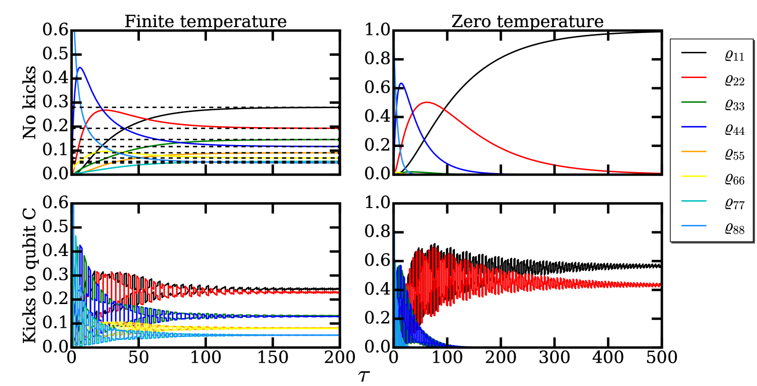
Figure 1: The figures shows the diagonal elements of the density matrix for: $\delta_{B}=0.5$, $\delta_{C}=0.25$, $\chi=0.15$, $\chi^{\prime}=0.1$ for the finite temperature limit ($D=1$) and the zero temerpature limit ($D=0$) and coupling strength to the bath $\beta=0.1$. The first row shows the case when no kicks are applied and the second row shows the case when periodic kicks are applied to qubit C with a kick strength of $\kappa=\pi/2$ and a period of the kicks of $\tau_{\mathrm{k}}=\pi/2$.

When no kicks are applied, the finite temperature limit yield stationary states corresponding to a Gibbs distribution (dashed black lines), and for the zero temperature limit the system reaches the ground state as a spontaneous emission process takes place. When kicks are applied to a single qubit (second row of figure 1), the system reaches a quasi stationary condition which is characterized by fluctuations around a certain averaged value. These fluctuations are seen in the figure as discontinuities happening at the moment when a kick is done.

The joint action of the bath and kicks generate stationary states that posses a certain degree of superposition as one can notice in the shortened distance between the diagonal elements associated to the transitions of the kicked qubit, eg. at the finite temperature limit and according to the quantum register defined as $|ABC\rangle$, the states $|AB0\rangle$ lie closer to the state $|AB1\rangle$, for $A,B=0,1$. This superposition is more noticeable at the zero temperature limit, (bottom left sub figure in 1), since now the effect of the bath is to drive the system to the ground state while the kicks pulls up the state corresponding to the superposition while the ground state is dragged down. In figure 2, the density matrices at the quasi stationary regime are plotted for the zero temperature limit and the finite temperature limit and when the kicks are done to the three different qubits. In this figure one notices that the coherent terms correspondent to the superposition of states of the kicked qubit have a non-zero value regardless the inherent decoherence induced by the bath.

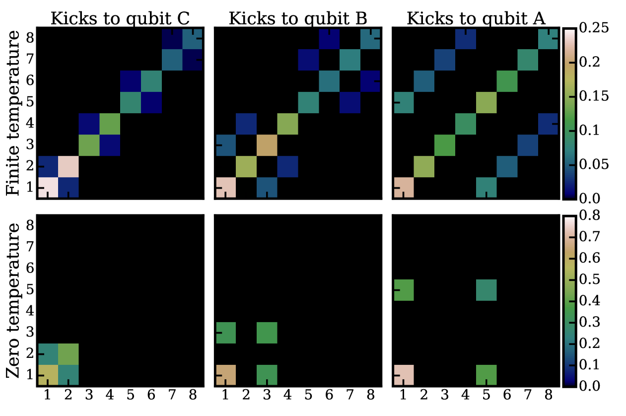
Figure 2: The figure shows the matrix elements of the matrix density of the linear chain for periodic kicks to qubit C B and A at the quasi stationary regime for kick strengths of: $\kappa=\pi/2$ and period of the kicks: $\tau_{\mathrm{k}}=\pi/2$, and $\delta_{B}=0.5$, $\delta_{C}=0.25$, $\chi=0.15$, $\chi^{\prime}=0.1$. The coupling strength to the bath is: $\beta=0.1$ and $D=1$ for the finite temperature case and $D=0$ for the zero temperature limit.

The superposition appearing in the system is in fact resilient to the environment as they are the result of both mechanism of dissipation and kicks acting together over the linear chain eg. when kicks are done to qubit A at the zero temperature limit (bottom right sub figure in figure 2), there is superposition between the state $|1\rangle=|000\rangle$ and the state $|5\rangle=|100\rangle$ which appears as a consequence of the bath attempting to drive the system to the ground state $|1\rangle=|000\rangle$ making it the most likely state while the action of repeated kicks to qubit A are always creating superpositions of states of qubit A thus, at the quasi stationary regime, the kicks are only acting on the ground state creating a superposition between this one and the state $|5\rangle=|100\rangle$ which is the state that corresponds to the single transition of qubit A. This explanation describes the resultant quasi steady states reached by the system when extrapolated to the cases when the other qubits are kicked and to the finite temperature limit where now the bath drives the system into a mixture of states (Gibbs distribution). We will discuss more about the super position states later on.

The quasi stationary regime is reached by the system when it enters into a cycle limit dynamics where the amount of of energy dissipated to the environment between two consecutive kicks equals the amount of energy received by the individual kicks. A profile of the energy of the system at the time $\tau$; $E(\tau)=\langle H_{\mathrm{s}}\rangle$ is depicted in figure 3 for the zero temperature and finite temperature limits. In the figure one sees the quasi stationary is reached after certain time where the energy fluctuates around a constant value.

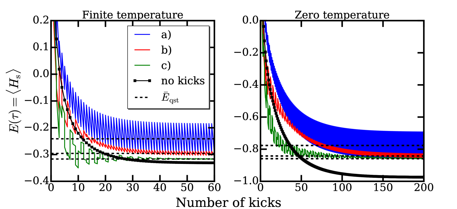
Figure 3: The figure shows the energy of the linear chain for the cases when: (no kicks) only the bath acts on the system, (a) kicks done to qubit A, (b) kicks done to qubit B and (c) kicks done to qubit C. The dashed black lines show the average energy of the quasi stationary state. The parameters used are $\kappa=\pi/2$, $\tau_{\mathrm{k}}=\pi$, $\delta_{B}=0.5$, $\delta_{C}=0.25$, $\chi=0.15$, $\chi^{\prime}=0.1$ and $\beta=0.1$.

It has been shown for the kicked oscillator and the kicked rotor that at the quasi stationary regime, these systems follows a Fourier’s law where the average energy of the systems and the dissipated energy to the environment per period of the kick are directly proportional, see eg. PrLoGo2016; Vázquez and García (2016). The averaged energy at the quasi stationary regime is defined as

$$\bar{E}_{\mathrm{qst}}=\lim_{n\rightarrow\infty}{E(\tau_{n}^{+})+E(\tau_{n}^{-})\over 2}$$ (8)

where $\tau_{n}^{+}=\lim_{\delta\rightarrow 0}n\tau_{\mathrm{k}}+\delta$ and $\tau_{n}^{-}=\lim_{\delta\rightarrow 0}n\tau_{\mathrm{k}}-\delta$ represents respectively the time immediately after and immediately before the n-th kick has happen. On the other hand, the dissipated energy per period of the kicks is defined as:

$$\delta Q/\tau_{\mathrm{k}}=\lim_{n\rightarrow\infty}{E(\tau_{n}^{+})-E(\tau_{n+1}^{-})\over\tau_{\mathrm{k}}}$$ (9)

For our system, we have found a similar behavior for the linear chain as one can sees from figure 4 where the averaged energy at the quasi stationary regime is plotted against the dissipated energy per period of the kick for kicks applied to qubit A.

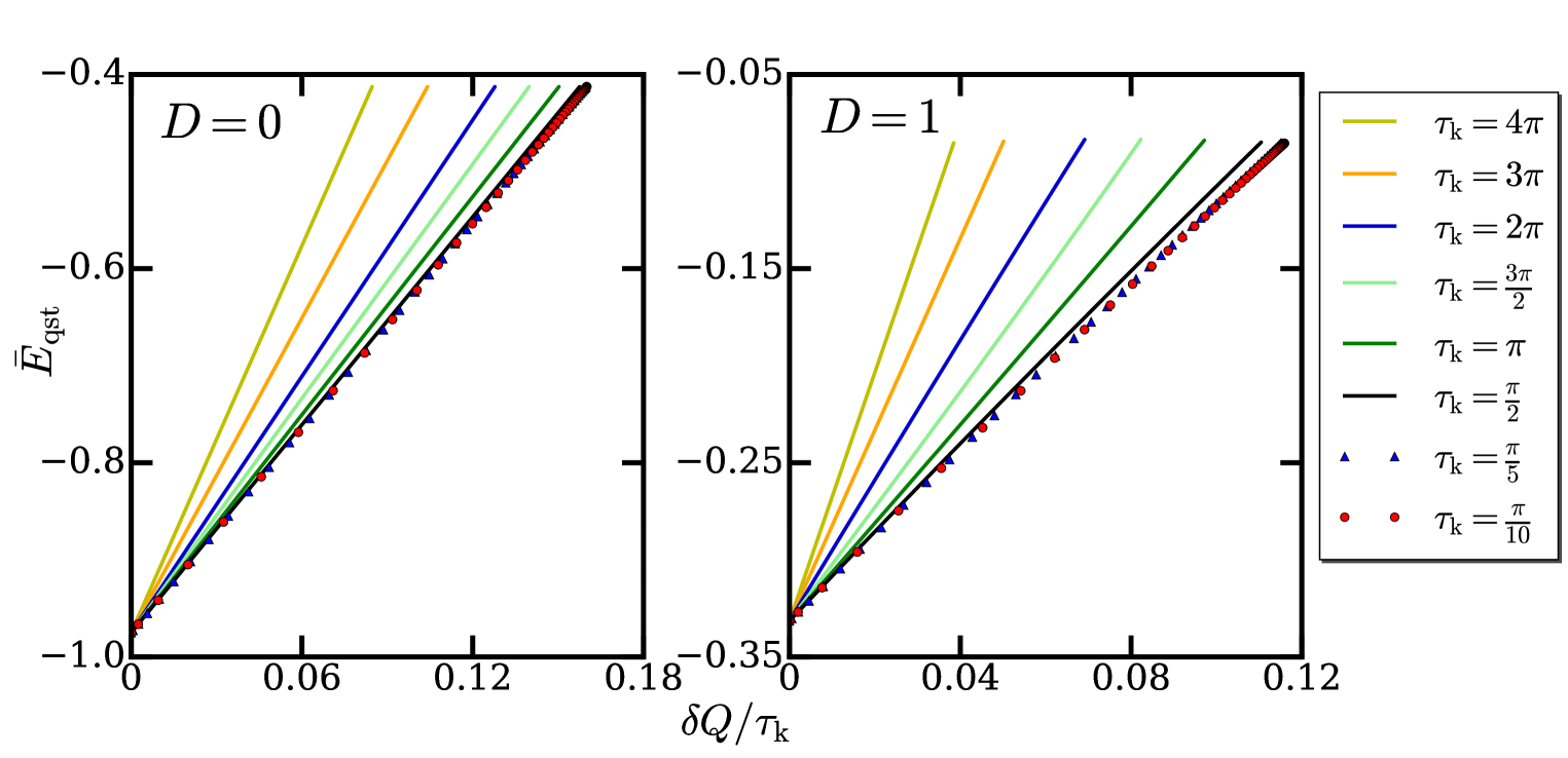
Figure 4: Linear relation between the averaged energy of the system and the energy dissipated to the environment per period of kicks at the quasi stationary regime when kicks are applied to qubit A. The figure shows the finite temperature and the zero temperature limit. The kick strength is varied from 0 to $2\pi$ and different periods of the kick have been used. The parameters of the linear chain are: $\delta_{B}=0.5$, $\delta_{C}=0.25$, $\chi=0.15$, $\chi^{\prime}=0.1$ and $\beta=0.1$.

As the period of the kicks becomes smaller (more frequent kicks) the proportionality of $\bar{E}_{\mathrm{qst}}$ to $\delta Q/\tau_{\mathrm{k}}$ becomes independent on the period of the kicks. The independence on the of the slope to the period of the kicks was observed in PrLoGo2016 for the kicked oscillator system where the slopes only depend on the damping rate. Nevertheless there is no fundamental reason why the slopes should not depend on the period of the kicks. If the kicks applied to the other two qubits, a similar behavior is observed as in figure 4 for the zero temperature limit. Nevertheless we have found for the finite temperature limit, certain cases where the relation does not seems to be linear anymore. This is shown in figure 5 where we have depicted the finite temperature limit when the kicks are applied to qubit B and qubit C.

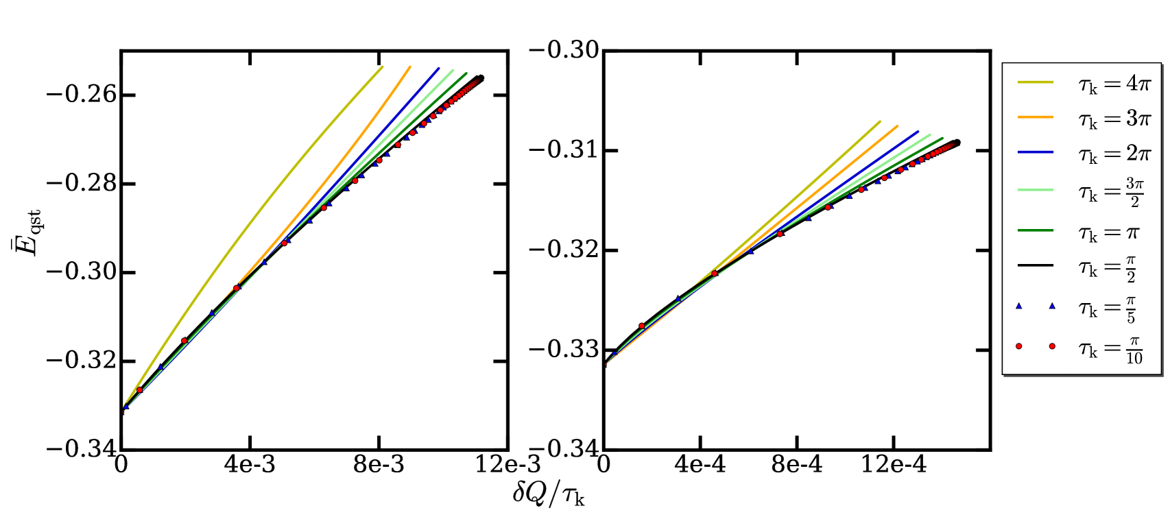
Figure 5: Relation between the averaged energy of the system and the energy dissipated to the environment per period of kicks at the quasi stationary regime when kicks are applied to qubit B (figure at the left) and C (figure at the right) for the finite temperature limit with $D=1$. The kick strength is varied from 0 to $2\pi$ and different periods of the kick have been used. The parameters of the linear chain are: $\delta_{B}=0.5$, $\delta_{C}=0.25$, $\chi=0.15$, $\chi^{\prime}=0.1$ and $\beta=0.1$.

Now we place our attention back to the coherences appearing at the quasi stationary states. The coherent terms are a consequence of the angle of rotation, $\kappa=\pi/2$, for which the kick instantaneously changes the states of the kicked qubits into a superposition of states, eg. if $n$th qubit is initially found in the state $|\psi\rangle_{n}=|0\rangle_{n}$, then the application of a kick into the $x$-direction will yield: $R_{x,n}^{\pi/2}|0\rangle_{n}=1/\sqrt{2}(|0\rangle_{n}+\mathrm{i}|1\rangle_{n})$. This superposition is kept in the system at a certain degree when the quasi steady condition is reached because of the repeated application of the kicks. There are other ways to generate superposition of states as a quasi stationary condition. One possible way is to apply first a kick corresponding to a rotation of $\pi$ along the $x$ axis and afterwards to apply a kick corresponding to a rotation of $\pi/2$ along the $y$ axis. This will change the state of the qubit $|\psi\rangle_{n}=|0\rangle_{n}$ into $R_{x,n}^{\pi}R_{y,n}^{\pi/2}|0\rangle_{n}=\mathrm{i}/\sqrt{2}(|0\rangle_{n}+|1\rangle_{n})$ which is the same superposed state but with a global constant phase.
Although a certain amount of coherence is gained in both cases, in general, the purity of the linear chain does not gets improved because the rest of the qubits of the linear chain are subjet to the influence of the bath alone producing decoherence on them. In figure 6 the purity, (first row), is plotted against the period of the kicks, for the cases where the kicks are done in the $x$ direction with an angle of $\pi/2$ (continuous lines) and when the kicks are done by an angle of $\pi$ in the $x$ direction and $\pi/2$ in the $y$ direction (dashed lines).

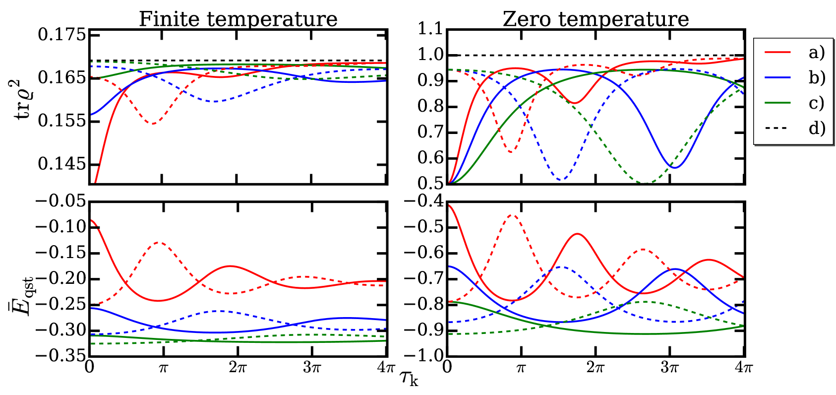
Figure 6: Purity of the system at the quasi stationary regime for the finite temperature ($D=1$) and the zero temperature ($D=0$) limits as a function of the period of the kicks when the kicks have been applied to a) qubit A, b) qubit B and c) qubit C. The continuous lines shows the purity when the kicks are done by an angle of $\pi/2$ around the $x$ axis and the dashes lines shows the purity when the kicks are done in a $\pi$ angle around the $x$ axis and $\pi/2$ angle around the $y$ axis. The dashed black lines labeled by d) represent the purity of the stationary state when only the bath acts on the system. The parameters of the linear chain are: $\delta_{B}=0.5$, $\delta_{C}=0.25$, $\chi=0.15$, $\chi^{\prime}=0.1$ and $\beta=0.1$.

One sees in the figure that the purity has a strong dependence on the period and the direction of the kicks presenting some local maximums and minimums at different periods of the kicks. At the second row of figure 6, the average energy at the quasi steady regime is plotted and it also increases and decreases as function of the period of the kicks meaning that the system passes through resonant and non-resonant regions. The resonant regions coincide with the periods of smaller purity and vice versa.

IV Simultaneous kicking and the emergence of stationary entanglement

Now we consider the scenario when simultaneous kicks are applied to different qubits. In this case, the application of the kicks produces non-local changes on the system which together with the effects of the bath into the system it is possible to obtain a certain degree of entanglement between the kicked qubits as a stationary condition. The entanglement produced among the qubits would be inherently resilient to the effects of the environment in the sense that the environment together with the application of kicks are the mechanism that produce it. We begin by showing in figure 7 the density matrices at the quasi stationary regime, when the kicks are simultaneously applied to two different qubits. In the figure, the kicks are applied in the $x$ direction with an angle of $\kappa=\pi/2$, such that the unitary operator representing the kicks is: $R_{x,i}^{\pi/2}R_{x,j}^{\pi/2}$ with $i\neq j$ labeling the different qubits.

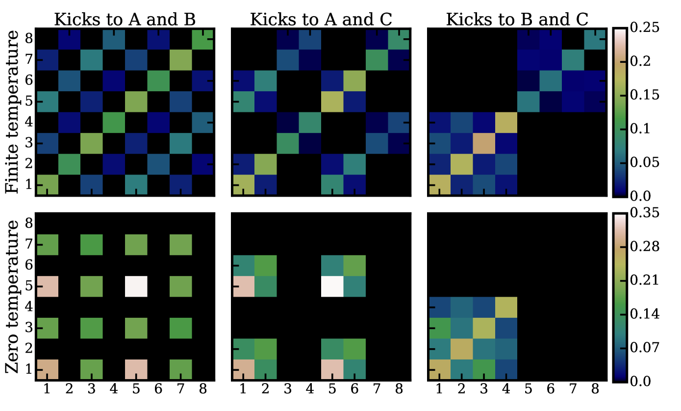
Figure 7: Density matrix at the quasi stationary regime for the finite temperature ($D=1$) and the zero temperature ($D=0$) for simultaneous kicking. The period of the kick used was $\tau_{\mathrm{k}}=4\pi$ and the kick strength was settled to $\pi/2$. The parameters of the linear chain are: $\delta_{B}=0.5$, $\delta_{C}=0.25$, $\chi=0.15$, $\chi^{\prime}=0.1$ and $\beta=0.1$.

The pattern formed at the quasi stationary state contains new superpositions of states which are the result of both mechanisms of kicks and dissipation, eg., in the sub figure at the bottom left, which shows the case for kicks done to qubits A and B at the zero temperature limit, the bath is always driving the system to the ground state which becomes the most likely state to be populated. On the other hand, the application of the kicks will have more influence over this state than any other, bringing the system into a non pure superposition states similar to: $|\psi\rangle\sim c_{1}|000\rangle+c_{3}|010\rangle+c_{5}|100\rangle+c_{7}|110\rangle$. This superposition pattern does not corresponds to a pure state because the environment is always acting on the system producing decoherence. Moreover, the decoherence makes the states of the system to be non separable and thus, a certain amount of entanglement between the qubits is induced. In order to measure the degree of entanglement we use the logarithmic negativity Plenio (2005) defined as:

$$E_{j}(\varrho)=\log_{2}\left(2\mathcal{N}_{j}+1\right)$$ (10)

where $\mathcal{N}_{j}$ is the negativity of the $j$-th qubit defined as:

$$\mathcal{N}_{j}=\sum_{i}{|\lambda_{ij}|-\lambda_{ij}\over 2}$$ (11)

and $\lambda_{ij}$ are eigenvalues of the partial transpose $\varrho^{\Gamma_{j}}$ of $\varrho$, with respect to the $j$ qubit. The logarithmic negativity will measure how much entangled is the $j$th qubit with the rest of the system. In figure 8 we show the logarithmic negativity for the cases shown in figure 7 (continuous lines), and another configuration of the kicks represented by the unitary operator $R_{x,j}^{\pi}R_{y,j}^{\pi/2}R_{x,i}^{\pi/2}$ with $i\neq j$ labeling the different kicked qubits, this is; one qubit is first kicked in the $x$ direction by an angle $\pi$ and afterwards in the $y$ direction by an angle $\pi/2$ while the other qubit is kicked in the $x$ direction by an angle $\pi/2$. This configuration is chosen because it produces higher rates of entanglement for certain periods of the kicks although, there might exist some other configurations of the kicks producing larger rates of entanglement between the qubits. Additionally, we only present the zero temperature limit case since for the finite temperature limit we have not found any entanglement between the qubits in the parameter regime explored so far.

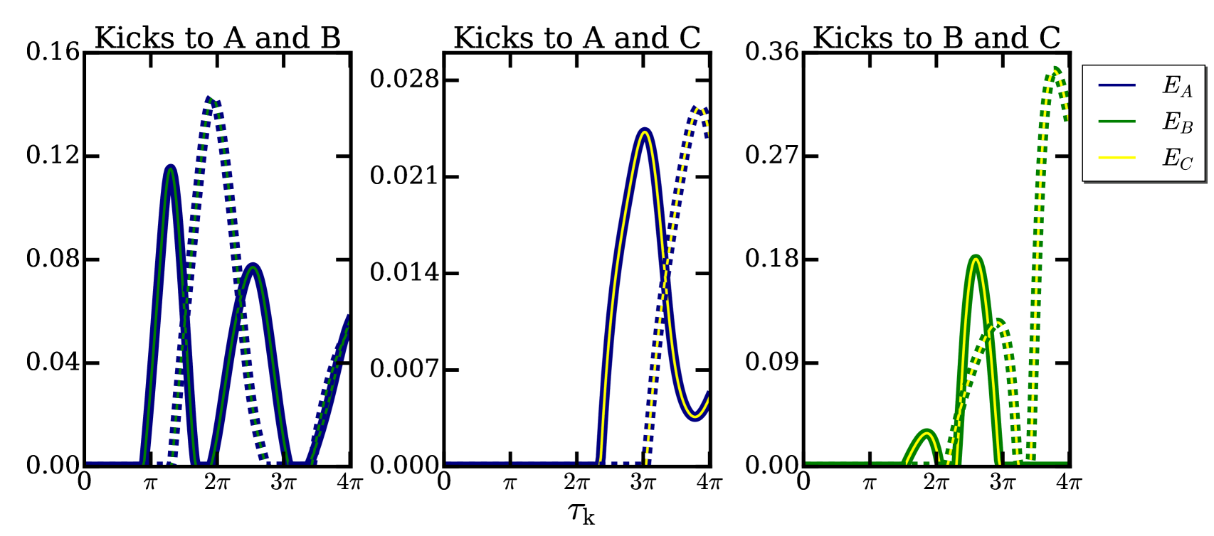
Figure 8: Logarithmic negativity of the qubits at the zero temperature limit ($D=0$) for simultaneous kicking as a function of the period of the kicks for the cases when the kicks are applied in the $x$ direction with an angle $\pi/2$ to two different qubits (continuous lines) and when the kicks are applied to one qubit first in the $x$ direction by an angle $\pi$ and afterwards in the $y$ direction by an angle $\pi/2$ while the other qubit is kicked in the $x$ direction by an angle $\pi/2$. The parameters of the linear chain are: $\delta_{B}=0.5$, $\delta_{C}=0.25$, $\chi=0.15$, $\chi^{\prime}=0.1$ and $\beta=0.1$.

In figure 8, one can observe that the largest rate of entanglement happens for the kicks done to qubit B and C which have a closer Larmor frequency among them. This suggest us one possible way to enhance entanglement by changing the configuration of the system, particularly by doing the Larmor frequencies of the kicked qubits, closer to each other. This can be physically realizable by letting the qubits to lie closer in the linear chain, since their Larmor frequencies are position dependent due to the gradient of the magnetic field field. In figure 9 we have plotted at the first row the logarithmic entanglement of qubits B and C as function of the period of the kicks, when kicks are done using different configurations and with the system parameters settled to: $\delta_{B}=0.26$, $\delta_{C}=0.25$, $\chi_{AB}=0.011$, $\chi_{AC}=0.1$, $\chi_{BC}=0.15$. Now we have independently defined the Ising interaction rate according to the distance between the qubits. Additionally at the second row we have plotted the ratio of the average energy at the quasi stationary state $\bar{E}_{\mathrm{qst}}$ and the dissipated energy to the environment per period of the kick $\delta Q/\tau_{\mathrm{k}}$ versus the period of the kick.

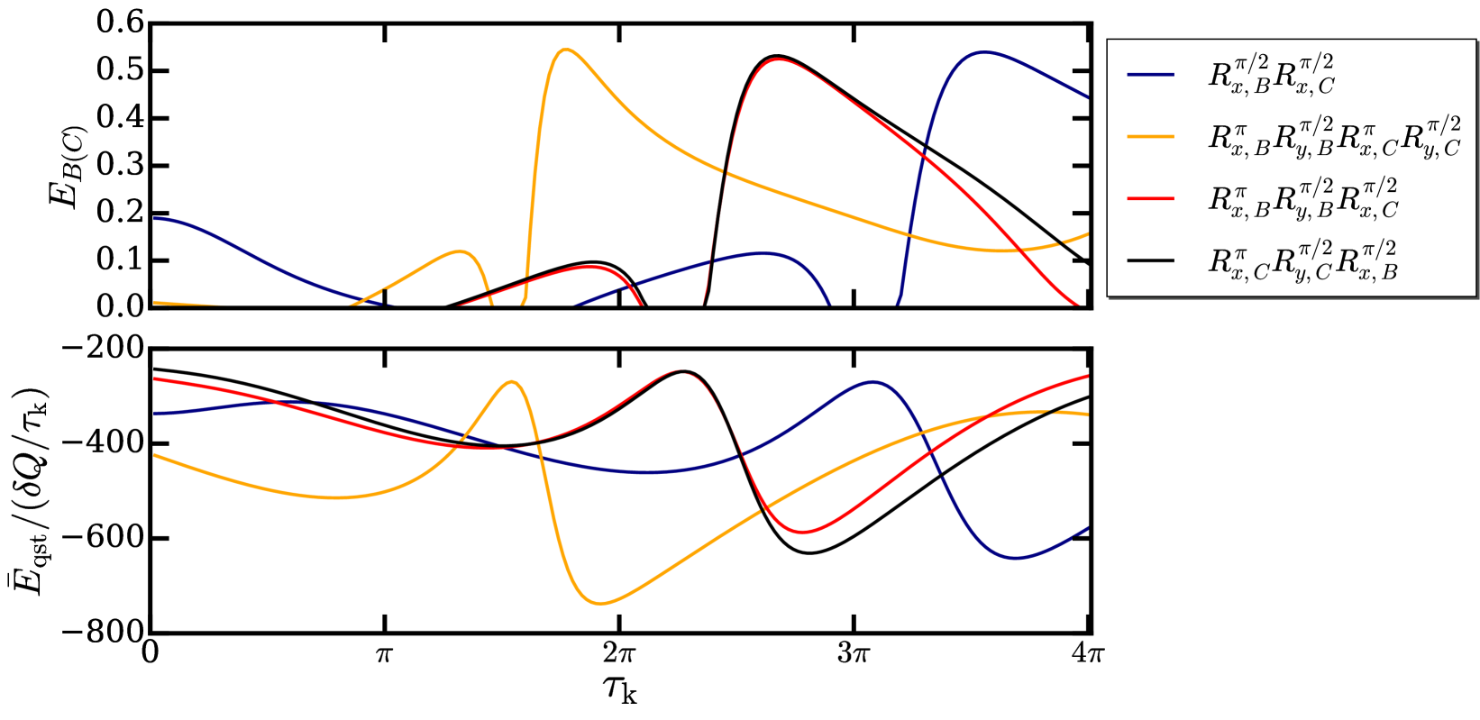
Figure 9: At the first row are plotted the logarithmic negativities of the qubits B and C at the zero temperature limit ($D=0$) for simultaneous kicking as a function of the period of the kicks with the kicks applied in different configurations At the second row are plotted the ratio between the average energy and the dissipated energy as a function of the period of the kicks for the correspondent cases considered at the first row. The parameters of the linear chain are: $\delta_{B}=0.26$, $\delta_{C}=0.25$, $\chi_{AB}=0.011$, $\chi_{AC}=0.1$, $\chi_{BC}=0.15$ and $\beta=0.1$.

Figure 9 shows that the maximum entanglement happens for periods of the kicks which corresponds to the global minimum of the ratio between the average energy and the dissipated energy per period of the kick. On the other hand, under the Fourier’s law assumption PrLoGo2016, the ratio between the average energy and the dissipated energy is equivalent in definition to a period dependent Fourier’s coefficient $\mathcal{F}(\tau_{\mathrm{k}})$ which describes the proportionality rate between the difference of temperatures between the system and the bath, and the energy exchange (dissipated energy) between the two systems $\Delta T=\mathcal{F}(\tau_{\mathrm{k}})\delta Q/\tau_{\mathrm{k}}$ (notice that at the zero temperature limit this difference corresponds only to the average energy of the system, $\Delta T\sim\bar{E}_{\rm{qst}}$). From the figure one notices that the Fourier’s coefficient and the entanglement seems to follow an inverse relation such that the maximum rates of entanglement between the qubits appear for periods of the kicks where the Fourier’s coefficient is minimum. We should mention that the formation of entangled states between certain qubits in a linear chain by means of periodic kicks has been explored before in Sainz et al. (2011), nevertheless in this case, the entanglement does not appears as a stationary condition and the interaction with the environment in fact will destroy it. In our case the formation of the stationary entanglement appears in the system due to the collective action of the mechanisms of dissipation and non local kicks in the linear chain. It may be possible to understand the formation of the entanglement as an emergent property of the system as it can be measured and classified as a property of a set of parts of the system which are in this case the two kicked qubits.

V Summary

We have described the quasi stationary condition reached by a linear chain made of qubits subject to periodic kicks and dissipation. The linear chain we have used has been a theoretical model for a certain type of quantum computing models. For doing our study we have derived a master equation for which the degree of interaction to the environment depends on the energy of the different states of the linear chain. This model of dissipation leads to a stationary condition which corresponds to a Gibbs distribution at the finite temperature limit and to the ground state at the zero temperature limit which are the limits one would expect. We have described the conditions and the attributes of the non-equilibrium stationary states reached by the system when periodic delta kicks are applied to the qubits in two different situations: kicks applied to single qubits and simultaneous kicks applied to the qubits. In the case of single kicked qubits, we have found an endurable condition of the system to remain in a superposition state regardless of the effects of the bath since the bath itself plays a crucial role in the formation of these states. Nevertheless we have found that the overall purity of the system does not gets improved since the rest of the linear chain remains under the influence of the bath. Also we have found resonant periods of the kicks for which the degree of super position and the average energy of the system increases. In the second case we have found the emergence of stationary entanglement when simultaneous kicks are applied to a pair of qubits of the linear chain. We have enhanced the rates of entanglement by changing the configuration of the system making the two kicked qubits to lie closer to each other and we observed that there exist an inverse relation between the entanglement and the Fourier’s coefficient of the system at the quasi stationary regime.

Appendix A Derivation of a master equation

In López and López (2011) a derivation of a master equation for a linear chain of three nuclear spins system with second neighbor Ising interaction has been done and also similar lines of derivation of a master equation has been done for the quantum planar rotor in Vázquez and García (2016). In both cases, the energy spectrum of the system has a non-equidistant spectrum and are coupled to the environment through creation and annihilation operators producing spontaneous emission and thermally induced processes. Here we follow similar lines of the derivation of both cases to derive the master equation that will account for our model. This master equation is not in a Lindblad form but rather it is derived by Redfield approximations which we consider to work better for the description of the spontaneous emission and thermally induced process on a system with an non-equidistant spectrum. We start by writing the full Hamiltonian of the composite in the form $H(t)=H_{\mathrm{c}}+W_{\mathrm{int}}(t)$ with $H_{\mathrm{c}}=H_{\mathrm{s}}+H_{\mathrm{env}}$ where $H_{\mathrm{env}}=\sum_{i}^{\infty}\hbar\omega_{i}a^{{\dagger}}_{i}a_{i},$ and $W_{\mathrm{int}}(t)=H_{\mathrm{rf}}(t)+H_{\mathrm{int}}$. The dynamical equation of the reduced density matrix for the spin chain system with an initially decoupled state of the system-environment, $\varrho=\varrho_{\mathrm{s}}\otimes\sigma_{\mathrm{env}}$, in the interaction picture with respect to $H_{\mathrm{c}}$, and under the Born-Markov limit Breuer and Petruccione (2002) can be written in the following form:

$${\mathrm{d}\tilde{\varrho}_{\mathrm{s}}(t)\over\mathrm{d}t} = {1\over\mathrm{i}\hbar}[\tilde{H}_{\mathrm{rf}}(t),\tilde{\varrho}_{\mathrm{s}}(t)]$$

$$\!\!-{1\over\hbar^{2}}\!\!\int_{0}^{\infty}\!\!\!\!\!\mathrm{d}\tau\mathrm{Tr}_{\mathrm{e}}[\tilde{H}_{\mathrm{int}}(t),[\tilde{H}_{\mathrm{int}}(t-\tau),\tilde{\varrho}_{\mathrm{s}}(t)\otimes\sigma_{\mathrm{e}}]].$$

The operators $\tilde{s}_{j}^{\pm}$ for $j=1,...,N$, in the interaction picture have the form:

$$\tilde{s}_{j}^{\pm}(t)=s^{\pm}_{j}e^{\pm i\hat{\Omega}_{j}t},$$ (13)

where

$$\hat{\Omega}_{j}=\omega_{j}+{J\over\hbar}(s_{j+1}^{z}+s_{j-1}^{z})+{J^{\prime}\over\hbar}(s_{j+2}^{z}+s_{j-2}^{z}),$$ (14)

is an frequency operator that commutes with the Hamiltonian $H_{\mathrm{s}}$ and whose eigenvalues are the transition frequencies of the different states. The interaction Hamiltonian between the spin chain and the environment is represented by a coupling between the polarization operator and a Bosonic modes operators. Since the baths are supposed to be in a stationary Boltzmann states: $\sigma_{\mathrm{e}}=\prod_{k}{1\over\mathcal{Z}}\sum_{n_{k}}\mathrm{e}^{-E_{n_{k}}/k_{B}T}|n_{k}\rangle\langle n_{k}|$, any perturbation thermalizes immediately and also the and also the self correlation functions of the baths are null: $\langle\hat{a}_{i}^{{\dagger}}(s)\hat{a}_{k}^{{\dagger}}(t)\rangle=\langle\hat{a}_{i}(s)\hat{a}_{k}(t)\rangle=0$. The bath correlation functions appearing in (A) have the following form:

$$\sum_{i,k}g_{ij}g^{*}_{kl}\mathcal{C}_{ik}(\tau) = \sum_{i}|g|^{2}_{ijl}\mathrm{e}^{-\mathrm{i}\omega_{i}\tau}\left(N(\omega_{i})+1\right)$$ (15)

$$\sum_{i,k}g^{*}_{ij}g_{kl}\mathcal{C}^{*}_{ik}(\tau) = \sum_{i}|g|^{2}_{ijl}\mathrm{e}^{i\omega_{i}\tau}N(\omega_{i}),$$ (16)

where $\mathcal{C}_{ik}(\tau)=\langle a_{i}(\tau)a^{{\dagger}}_{k}\rangle$, $\mathcal{C}_{ik}(\tau)^{*}=\langle a_{i}^{{\dagger}}(\tau)a_{k}\rangle$ and $N(\omega_{i})=\left(\mathrm{e}^{\omega_{i}\hbar/k_{B}T}-1\right)^{-1}$ are the Planck’s distribution function. We assume the sum over $i$ is dense (there are an uncountable number of radiation modes) and the continuous limit can be taken. The number of characteristic frequencies with wave vector components $\vec{f}$ in the interval $\mathrm{d}f_{x}\mathrm{d}f_{y}\mathrm{d}f_{z}$ in the volume $V$ is given by $V4\pi f^{2}\mathrm{d}f/(2\pi)^{3}={V\omega^{2}}\mathrm{d}\omega/\pi^{2}c^{3}$, where $f=c\cdot\omega$. Thus the sum in the correlation functions can be changed by an integration over the frequencies with the proper weight factor,

$$\sum_{i,k}g_{ij}g^{*}_{kl}\mathcal{C}_{ik}(\tau) = {\gamma_{jl}\over\pi}\int_{-\infty}^{\infty}\!\!\!\!\mathrm{d}\omega\,\omega^{3}(N(\omega)+1)e^{-\mathrm{i}\omega\tau}$$ (17)

$$\sum_{i,k}g^{*}_{ij}g_{kl}\mathcal{C}^{*}_{ik}(\tau) = {\gamma_{jl}\over\pi}\int_{-\infty}^{\infty}\!\!\!\!\mathrm{d}\omega\,\omega^{3}N(\omega)e^{\mathrm{i}\omega\tau}$$ (18)

where $\gamma_{jl}={V|g|^{2}_{jl}/\pi c^{3}}$. The correlation functions becomes the Fourier transform of a spectral density associated to the continuous modes in the thermal bath and we have assumed a linear dependence on the characteristic frequencies of the radiation modes, $|g|_{ijl}^{2}=|g|^{2}_{jl}\omega_{i}$. By writing equation (A) back in the Schrödingers picture and using (17) and (18), we write for the master equation:

$${\mathrm{d}\varrho_{\mathrm{s}}(t)\over\mathrm{d}t} = {1\over\mathrm{i}\hbar}[H_{\mathrm{s}}+H_{\mathrm{rf}}(t),\varrho_{\mathrm{s}}]$$

$$\!\!-{1\over\hbar^{2}}\!\!\sum_{j,l=1}^{N}{\gamma_{jl}\over\pi}\int_{0}^{\infty}\!\!\!\!\!\mathrm{d}\tau\!\!\int_{-\infty}^{\infty}\!\!\!\!\!\mathrm{d}\omega\,\omega^{3}\,\mathcal{R}_{j,l}(\omega,\tau)[\varrho_{\mathrm{s}}]$$

where the super operator $\mathcal{R}_{j,l}(\omega,\tau)[\varrho_{\mathrm{s}}]$ is defined as

$$\mathcal{R}_{j,l}(\omega,\tau)[\varrho_{\mathrm{s}}] = \left(N(\omega)+1\right)\mathrm{e}^{-\mathrm{i}\left(\omega-\hat{\Omega}_{l}\right)\tau}\mathrm{D}_{1}[\varrho_{\mathrm{s}}]$$ (20)

$$+N(\omega)\mathrm{e}^{\mathrm{i}\left(\omega-\hat{\Omega}_{l}\right)\tau}\mathrm{D}_{2}[\varrho_{\mathrm{s}}]+h.c.$$

with $\mathrm{D}_{1}[\varrho_{\mathrm{s}}]=s_{j}^{+}s_{l}^{-}\varrho_{\mathrm{s}}-s_{l}^{-}\varrho_{\mathrm{s}}s_{j}^{+}$ and $\mathrm{D}_{2}[\varrho_{\mathrm{s}}]=s_{j}^{-}s_{l}^{+}\varrho_{\mathrm{s}}-s_{l}^{+}\varrho_{\mathrm{s}}s_{j}^{-}$. Now we can exchange the order of integration in (A) and evaluate the integrals by introducing a full eigenbasis of $H_{\mathrm{s}}$, lets say $\mathbb{I}=\sum_{m}|m\rangle\langle m|$ and call $\Omega_{lm}$, the eigenvalues of the operator $\hat{\Omega}_{l}$, ($\hat{\Omega}_{l}|m\rangle=\Omega_{lm}|m\rangle$), for the jth spin. For the $\tau$ integration we can separate the real and the imaginary part by using the known relation $\int_{0}^{\infty}\mathrm{d}\tau\mathrm{e}^{\pm\mathrm{i}\epsilon\tau}=\pi\delta(\epsilon)\mp\mathrm{i}{\mathbf{P}/\epsilon}$, where $\mathbf{P}$ is the Cauchy’s principal value. For the real part, integration over $\tau$ will yield delta functions of the form $\delta(\omega-\Omega_{lm})$. Consequently, integration over $\omega$ will yield : $\int_{-\infty}^{\infty}\,\mathrm{d}\omega\,\delta\left(\omega-\Omega_{lm}\right)\omega^{3}N\left(\omega\right)=\Omega^{3}_{l}\,N(\Omega_{lm})$. This real part is responsible of the non-unitary dynamics of the system yielding the dissipative processes and thermalization processes. On the other hand, the imaginary part contain some non physical contributions to the dynamics that can be solved if we neglect a small term under the assumption of $\omega_{l}\gg J(J^{\prime})\hbar$ and additionally assume the secular approximation which is equivalent to consider $\gamma_{ij}=\gamma_{i}\delta_{ij}$. With this assumptions the imaginary term can be incorporated to the von Neumann dynamics. By recovering the identity we write for the master equation:

$$\mathrm{i}\hbar{\mathrm{d}\varrho_{\mathrm{s}}(t)\over\mathrm{d}t}=[H_{\mathrm{s}}+H_{\mathrm{rf}}(t)+H_{LS},\varrho_{\mathrm{s}}]+{\mathrm{i}\over\hbar}\mathcal{D}[\varrho_{\mathrm{s}}]\\$$

where

$$\mathcal{D}[\varrho_{\mathrm{s}}] = -\sum_{l=1}^{N}\left(\left[\hat{\mathrm{O}}^{(1)}_{l}\!(T)\,s_{l}^{+},s_{l}^{-}\varrho_{\mathrm{s}}\right]+\left[\varrho_{\mathrm{s}}s_{l}^{+},s_{l}^{-}\,\hat{\mathrm{O}}^{(1)}_{l}\!(T)\right]\right.$$

$$+\left.\left[\hat{\mathrm{O}}^{(2)}_{l}\!(T)\,s_{l}^{-},s_{l}^{+}\varrho_{\mathrm{s}}\right]+\left[\varrho_{\mathrm{s}}s_{l}^{-},s_{l}^{+}\,\hat{\mathrm{O}}^{(2)}_{l}\!(T)\right]\right)$$

with

$$\hat{\mathrm{O}}^{(1)}_{l}(T) = \gamma_{l}\hat{\Omega}_{l}^{3}\left(N(\hat{\Omega}_{l},T)\!+\!1\right)\,,$$ (22)

$$\hat{\mathrm{O}}^{(2)}_{l}(T) = \gamma_{l}\hat{\Omega}_{l}^{3}N(\hat{\Omega}_{l},T),$$ (23)

and

$$N(\hat{\Omega}_{l},T)=\left(\mathrm{e}^{{\hat{\Omega}_{l}\hbar/k_{B}T}}-1\right)^{-1}$$ (24)

with $\hat{\Omega}_{l}$ given by (14). The new term included in the von Neumann dynamics, $H_{LS}$ is:

$$H_{LS}=\sum_{l=1}^{N}\left(\hat{\Gamma}^{(1)}_{l}(T)s_{l}^{+}s_{l}^{-}+\hat{\Gamma}^{(2)}_{l}(T)s_{l}^{-}s_{l}^{+}\right)$$ (25)

with

$$\hat{\Gamma}^{(1)}_{l}(T) = {\gamma_{l}\over\pi\hbar}\int_{-\infty}^{\infty}\mathrm{d}\omega{\omega^{3}\left(N(\omega)+1\right)\over\omega-\hat{\Omega}_{l}},$$ (26)

$$\hat{\Gamma}^{(2)}_{l}(T) = {\gamma_{l}\over\pi\hbar}\int_{-\infty}^{\infty}\mathrm{d}\omega{\omega^{3}N(\omega)\over\omega-\hat{\Omega}_{l}}.$$ (27)

The term $\mathcal{D}[\varrho_{\mathrm{s}}]$ in (A) describes spontaneous emission and thermally induced process which occur at a rate that depends on the energy level distribution of the spin chain and the correlation of these process for the different spins. The transition probabilities of the system due to the spontaneous emission process occur with rates that depends on the cubic power of the energy level difference of each spin, $\approx\gamma_{l}\hat{\Omega}^{3}_{l}$ while the probability of increasing energy states due to the thermally induced processes occur with a rate of $\gamma_{l}\hat{\Omega}^{3}_{l}N(\hat{\Omega}_{l})$ which decays exponentially for large energy states. On the other hand the term $H_{LS}$ in (25) commutes with the Hamiltonian of the system and contributes with a certain shift to the eigen energies of the system. Typically this term is related to a Lamb shift effect and sometimes is simply neglected. This will be our case since we want to focus only on the non unitary dynamics effects of the bath. The zero temperature limit is considered when the temperature of the bath is sufficiently small compared to the energy transitions of the linear chain and one can do the limit $T\rightarrow 0$ in the operators (22) and (23) with (24). In this case, the dissipative term of the master equation describes a pure spontaneous emission process and the super operator responsible of the dissipation $\mathcal{D}[\varrho_{\mathrm{s}}]$ takes the form:

$$\mathcal{D}[\varrho_{\mathrm{s}}] = -\sum_{l=1}^{N}\gamma_{l}\left\{\left[\hat{\Omega}^{3}_{l}\,s_{l}^{+},s_{l}^{-}\varrho_{\mathrm{s}}\right]+\left[\varrho_{\mathrm{s}}\,s_{l}^{+},s_{l}^{-}\,\hat{\Omega}^{3}_{l}\right]\right\}.$$

At the finite temperature limit, the system reaches a stationary state which is a Gibbs distribution mixture of states and as the temperature increases the states get closer together until it reaches an homogeneous mixture for infinite temperatures. At the zero temperature limit, the system reaches a stationary state which is a pure state as in the spontaneous emission process where all the states become populated during the transients and in the long time limit only the ground state becomes populated.

References

- Haken (1970) H. Haken, “Laser theory,” in Light and Matter Ic / Licht und Materie Ic, edited by L. Genzel (Springer Berlin Heidelberg, Berlin, Heidelberg, 1970) pp. 1–304.
- Haken (2004) H. Haken, Synergetics, Introduction and Advanced Topics (Springer, 2004).
- Lutz and Weidenmüller (1999) E. Lutz and H. A. Weidenmüller, Physica A 267, 354 (1999).
- Gorin and Seligman (2002) T. Gorin and T. H. Seligman, J. Opt. B: Quantum Semiclass. Opt. 4, S386 (2002), topical issue: Mysteries and Paradoxes in Quantum Mechanics IV Quantum interference phenomena (Workshop held at Gargano, Italy, August 2001).
- Carrera et al. (2014) M. Carrera, T. Gorin, and T. H. Seligman, Phys. Rev. A 90, 022107 (2014).
- Moreno et al. (2015) H. J. Moreno, T. Gorin, and T. H. Seligman, Phys. Rev. A 92, 030104 (2015).
- Langemeyer and Holthaus (2014) M. Langemeyer and M. Holthaus, Phys. Rev. E 89, 012101 (2014).
- Ketzmerick and Wustmann (2010) R. Ketzmerick and W. Wustmann, Phys. Rev. E 82, 021114 (2010).
- Prado Reynoso et al. (2017) M. A. Prado Reynoso, P. C. López Vázquez, and T. Gorin, Phys. Rev. A 95, 022118 (2017).
- Vázquez and García (2016) P. C. L. Vázquez and A. García, Physica Scripta 91, 055101 (2016).
- Gardiner et al. (1997) S. A. Gardiner, J. I. Cirac, and P. Zoller, Phys. Rev. Lett. 79, 4790 (1997).
- Billam and Gardiner (2009) T. P. Billam and S. A. Gardiner, Phys. Rev. A 80, 023414 (2009).
- Dana and Dorofeev (2005) I. Dana and D. L. Dorofeev, Phys. Rev. E 72, 046205 (2005).
- Elyutin and Rubtsov (2008) P. V. Elyutin and A. N. Rubtsov, J. Phys. A 41, 055103 (2008).
- Fishman et al. (1982) S. Fishman, D. R. Grempel, and R. E. Prange, Phys. Rev. Lett. 49, 509 (1982).
- Anderson (1978) P. W. Anderson, Rev. Mod. Phys. 50, 191 (1978).
- Ad Lagendijk and Wiersma (2009) B. v. T. Ad Lagendijk and D. S. Wiersma, Physics Today 62 (2009).
- Berman et al. (2000) G. P. Berman, G. D. Doolen, G. V. López, and V. I. Tsifrinovich, Phys. Rev. A 61, 062305 (2000).
- López et al. (2003) G. V. López, J. Quezada, G. P. Berman, G. D. Doolen, and V. I. Tsifrinovich, J Opt B Quantum Semiclassical Opt 5, 184 (2003).
- Viola and Lloyd (1998) L. Viola and S. Lloyd, Phys. Rev. A 58, 2733 (1998).
- Rego et al. (2009) L. G. Rego, L. F. Santos, and V. S. Batista, Annual Review of Physical Chemistry 60, 293 (2009).
- Uhrig (2008) G. S. Uhrig, New Journal of Physics 10, 083024 (2008).
- Morton et al. (2006) J. J. L. Morton, A. M. Tyryshkin, A. Ardavan, S. C. Benjamin, K. Porfyrakis, S. A. Lyon, and G. A. D. Briggs, Nat Phys 2, 40 (2006).
- Liu et al. (2013) G.-Q. Liu, H. C. Po, J. Du, R.-B. Liu, and X.-Y. Pan, Nature Communications 4, 2254 (2013).
- López and López (2011) G. V. López and P. López, J. Mod. Phys. 3, 85 (2011).
- López and López (2012) P. C. López and G. V. López, J. Mod. Phys. 3, 902 (2012).
- Breuer and Petruccione (2002) H. P. Breuer and F. Petruccione, The Theory of Open Quantum Systems (Oxford University Press, USA, 2002).
- Pasini et al. (2008) S. Pasini, T. Fischer, P. Karbach, and G. S. Uhrig, Phys. Rev. A 77, 032315 (2008).
- Plenio (2005) M. B. Plenio, Phys. Rev. Lett. 95, 090503 (2005).
- Sainz et al. (2011) I. Sainz, G. Burlak, and A. B. Klimov, The European Physical Journal D 65, 627 (2011).