Recover Subjective Quality Scores from Noisy Measurements

Abstract

Simple quality metrics such as PSNR are known to not correlate well with subjective quality when tested across a wide spectrum of video content or quality regime. Recently, efforts have been made in designing objective quality metrics trained on subjective data (e.g. VMAF), demonstrating better correlation with video quality perceived by human. Clearly, the accuracy of such a metric heavily depends on the quality of the subjective data that it is trained on. In this paper, we propose a new approach to recover subjective quality scores from noisy raw measurements, using maximum likelihood estimation, by jointly estimating the subjective quality of impaired videos, the bias and consistency of test subjects, and the ambiguity of video contents all together. We also derive closed-from expression for the confidence interval of each estimate. Compared to previous methods which partially exploit the subjective information, our approach is able to exploit the information in full, yielding tighter confidence interval and better handling of outliers without the need for z-scoring or subject rejection. It also handles missing data more gracefully. Finally, as side information, it provides interesting insights on the test subjects and video contents.

1 Introduction

In video coding research and development, two methods have generally been used to evaluate the quality of impaired videos: subjective assessment through viewer experiments and objective assessment using quality metrics. Subjective assessment is the ultimate measure of viewer’s perception of quality, but is usually expensive to conduct. Very often, objective assessment is used as an alternative or complement to report perceptual quality. Peak-signal-to-noise-ratio (PSNR) and Structural Similarity Index (SSIM) [1] are examples of objective quality metrics originally designed for images but later extended to video. Besides, an objective quality metric can also be used as an optimization objective function, such as in per-title encode optimization [2] and per-scene encode optimization under bitrate and video buffer constraints.

Simple metrics such as PSNR find success in evaluating small differences and close performance among codecs or coding tools. However, it is well known that they do not correlate well with quality perceived by human when tested across a wide spectrum of quality or content. Recently, efforts have been made in addressing this issue by designing objective quality metrics through subjective data fusion (VMAF, FVQA, VQM-VFD) [3, 4, 5]. The basic idea is to extract low-level features or elementary metrics that are quality-indicative, and then use a machine-learning regressor, such as a support vector machine (SVM) [6] or a neural net, to fuse them into a “meta-metric” that makes a final prediction. The regressor model is trained using subjective data, such as mean opinion scores (MOS) aggregated over the raw opinion scores collected from subjective experiments. It is shown that the fusion-based approach correlates better with subjective data than other approaches [3].

Clearly, the accuracy of a fusion-based metric heavily depends on the quality of the subjective data that it is trained on. Thus, it is very important to provide clean and reliable training data. On the other hand, raw opinion scores offered by viewers are often noisy and unreliable, due to the following reasons:

• Subject bias. The notion of quality is highly subjective and test subjects are entitled to rate the videos in their own opinions. For example, more picky viewers tend to be biased toward lower scores, and vice versa. Also, not every subject has “golden eyes” – their sensitivity to impairments varies.

• Subject inconsistency. Subjective testing is a laborious process, and not every viewer can maintain attentiveness throughout. Some tend to rate more consistently than others.

• Content ambiguity. Some contents tend to be more difficult to be rated than others. For example, water surface with ripples in the dark is more ambiguous than a bright blue sky.

• Outliers. Last but not least, some raw scores are simply outliers – viewers may just not pay attention. Software issues may also render scores meaningless.

Existing approaches address some of the issues above. For example, MOS averages the raw scores from a number of subjects to produce an aggregate score, compensating for the bias and inconsistency of individuals. Z-score transformation (or z-scoring) [7] normalizes the scores on a per-subject basis. Subject rejection [8] counts the number of instances when a subject’s rating looks like an outlier, and if this occurs too often, the subject and all his or her scores are rejected.

In this paper, we propose a new approach to recover subjective quality scores from the noisy raw opinion measurements, by jointly estimating the subjective quality of impaired videos, the bias and consistency of test subjects, and the ambiguity of video contents all together. We propose a generative model that incorporates random variables representing each of these factors, cast the problem as maximum likelihood estimation (MLE), and derive a solution based on belief propagation (BP) [9]. We also derive closed-form expression for the confidence interval of each estimate based on Cramer-Rao bound [10]. Compared to previous methods which partially exploit the subjective information, our approach is able to exploit the information in full, yielding better handling of outliers without the need for z-scoring or subject rejection. The resulting estimated subjective scores have a tighter confidence interval compared to conventional approaches. It also handles missing data more gracefully. Lastly, as side information, it provides interesting insights on the test subjects and video contents.

The rest of the paper is organized as follows. Section 2 discusses related work. Section 3 defines the problem and notations. Section 4 describes traditional approaches, and Section 5 presents the proposed approach. Experimental results are reported in Section 6.

This work’s open-source implementation can be found at [11].

2 Related Work

The ITU-R BT.500 Recommendation [8] defines procedures for video subjective testings including both single-stimulus and double-stimulus methods. It also defines the method for subjective rejection. The ITU-T P.910 Recommendation [12] defines procedures for calculating differential MOS. Z-score transformation of subjective scores is proposed in [7] as a pre-processing step prior to subject rejection.

A theoretical model for subjects’ influence on test scores is proposed in [13], which is similar in spirit to ours. The authors have focused on validating the model using real data, which also provides support for this work. However, they have relied on repetitive experiments for model parameter estimation, while our proposed solution based on BP is much more efficient.

Recovering subjective quality scores from noisy measurements is closely related to the task of label inference from very large databases of hand labeled images. To address the label inference problem, [14] proposes a solution based on probablistic graphical model. [15] further extends the idea to the task of image quality evaluation. There is a number of differences between their approach and this work. First, they formulate a classification problem whereas this work considers a regression problem, which is closer to the nature of subjective test procedure considered. Second, their work adopts a discriminative model whereas this work adopts a generative model, allowing better interpretability of results.

3 Preliminaries

Consider an experiment with $S$ subjects, indexed by $s=1,...,S$, and $E$ impaired video encodes, indexed by $e=1,...,E$. For simplicity, we consider the case of a single viewing session with no repititions. A subject $s$ rates an impaired video encode $e$, producing a raw opinion score $x_{e,s}$. In the full sampling scenario, every subject rates every impaired video. In the selective sampling scenario, not every subject needs to rate every impaired video – if a score is missing, it is denoted by $x_{e,s}=*$. In the rest of the paper, unless otherwise stated, the full sampling scenario is assumed.

The raw opinion scores may be produced using different test methods, including both single-stimulus and double-stimulus methods: In absolute category rating (ACR), the subject is instructed to watch the impaired video and give a rating on the scale from 1 (quality is bad) to 5 (quality is excellent). In degradation category rating (DCR), the subject is instructed to watch a pair of videos – the unimpaired reference video followed by the impaired video, and then rate the impaired video on the scale from 1 (impairments are very annoying) to 5 (impairments are imperceptible). In either method, unimpaired hidden reference videos may be present along with other impaired videos, and are also rated by the subject. A differential score between the score of the impaired and its hidden reference may be used in place of the raw opinion score, and the resulting MOS calculated is called differential MOS (or DMOS) [12]. DMOS is useful when the quality degradation from the reference is relevant, rather than the absolute quality when, for example, the reference video is not perfect in quality.

Each impaired video $e$ is also associated with a content $c$, denoted by $c=\mathsf{c}(e)$, with $c=1,...,C$ where $C$ is the total number of video contents used in the experiment.

Throughout the paper, we use $\mu_{e}$ and $\mu_{s}$ to denote the mean values calculated over scores for impaired video $e$ and for subject $s$, respectively, i.e., $\mu_{e}=\frac{1}{S}\sum_{s}x_{e,s}$ and $\mu_{s}=\frac{1}{E}\sum_{e}x_{e,s}$. Similarly, $m_{n,e}$ and $m_{n,s}$ denote the $n$-th order central moment over scores for $e$ and $s$, respectively, i.e., $m_{n,e}=\frac{1}{S}\sum_{s}(x_{e,s}-\mu_{e})^{n}$ and $m_{n,s}=\frac{1}{E}\sum_{e}(x_{e,s}-\mu_{s})^{n}$. As special case, the standard deviation over scores for $e$ and $s$ have the form $\sigma_{e}=\sqrt{m_{2,e}}$ and $\sigma_{s}=\sqrt{m_{2,s}}$, respectively.

4 Traditional Approaches

The most basic approach to recover subjective quality scores from the raw opinion measurements is by averaging, or MOS: $x_{e}=\mu_{e}$, for impaired video $e=1,...,E$. Before the averaging step, one can apply the following:

Z-score transformation. It is advocated that the scores undergo a normalization procedure on a per-subject basis [7], i.e., $x_{e,s}\leftarrow\frac{x_{e,s}-\mu_{s}}{\sigma_{s}}$. Applying z-scoring could compensate for individual subject’s bias and inconsistency, preparing for favorable conditions for subject rejection. However, after z-scoring, the original scale of the scores is unfavorably lost, leading to difficulty in interpreting the results. Also, it only partially compensates for the influence of subjects. A theoretical analysis on z-scoring can be found in Appendix A.

Subject rejection. In [8], a recommendation for subject rejection is provided. The algorithm is reproduced in Algorithm 1 for completeness. Video by video, the algorithm counts the number of instances when a subject’s opinion score deviates by a few sigmas, and reject the subject if the occurences are more than a fraction. All scores corresponding to the rejected subjects are discarded, which could be an overkill.

• Input: $x_{e,s}$ for $s=1,...,S$ and $e=1,...,E$.

• Initialize $p(s)\leftarrow 0$ and $q(s)\leftarrow 0$ for $s=1,...,S$.

• For $e=1,...,E$:

  • Let $Kurtosis_{e}=\frac{m_{4,e}}{m_{2,e}^{2}}$.

  • If $2\leq Kurtosis_{e}\leq 4$, then $\epsilon_{e}=2$; otherwise $\epsilon_{e}=\sqrt{20}$.

  • For $s=1,...,S$:

    • If $x_{e,s}\geq\mu_{e}+\epsilon_{e}\sigma_{e}$, then $p(s)\leftarrow p(s)+1.$

    • If $x_{e,s}\leq\mu_{e}-\epsilon_{e}\sigma_{e}$, then $q(s)\leftarrow q(s)+1$.

• Initialize $Set_{rej}=\emptyset$.

• For $s=1,...,S$:

  • If $\frac{p(s)+q(s)}{E}\geq 0.05$ and $\left|\frac{p(s)-q(s)}{p(s)+q(s)}\right|<0.3$, then $Set_{rej}\leftarrow Set_{rej}\cup\{s\}.$

• Output: $Set_{rej}$.

Algorithm 1 Subject rejection [8]

5 Proposed Approach

In this section, we describe the proposed approach of jointly estimating the subjective quality of impaired videos, the bias and consistency of subjects, and the ambiguity of video contents. Different from traditional approaches which require an explicit z-score transformation or a subject rejection step, the proposed model naturally accounts for subjective biases, inconsistencies and outliers.

5.1 The Model

We model the raw opinion scores as a random variable $\{X_{e,s}\}$ with the following form:

$$X_{e,s} = x_{e}+B_{e,s}+A_{e,s},$$ (1)

$$B_{e,s} \sim \mathcal{N}(b_{s},v_{s}^{2}),$$

$$A_{e,s} \sim \mathcal{N}(0,a_{c:\mathsf{c}(e)=c}^{2})$$

for $e=1,...,E$ and $s=1,...,S$. In this model, $x_{e}$ represents the quality of impaired video $e$ perceived by an average viewer, $B_{e,s}$, $e=1,...,E$ are i.i.d. Gaussian variables representing the factor of subject $s$, and $A_{e,s}$, $s=1,...,S$ and $e:\mathsf{c}(e)=c$ are i.i.d. Gaussian variables representing the factor of video content $c$ (i.e., the content that $e$ corresponds to). The parameters $b_{s}$ and $v_{s}^{2}$ represent the bias (i.e., mean) and inconsistency (i.e., variance) of subject $s$, $s=1,...,S$. The parameter $a_{c}^{2}$ represents the ambiguity (i.e., variance) of content $c$, $c=1,...,C$. In this formulation, the unknowns are the model parameters $\theta=(\{x_{e}\},\{b_{s}\},\{v_{s}\},\{a_{c}\})$, where $\{\cdot\}$ denotes the corresponding set. The main idea of our approach is to jointly recover these unknowns by MLE. Let $L=\log P(\{x_{e,s}\}|\theta)$ be the log likelihood function, the goal is to solve for $\hat{\theta}=\arg\max_{\theta}L$. Our ultimate goal is to recover the estimated scores $\{x_{e}\}$ of a hypothetical unbiased and consistent viewer, while $\{b_{s}\}$, $\{v_{s}\}$ and $\{a_{c}\}$ are side information about the subjects and video contents. An analysis of the observations and unknowns in (1) and its recoverability can be found in Appendix B.

5.2 Belief Propagation

We derive a solution for the MLE formulation using BP algorithm. We start with the log-likelihood function. By (1), $X_{e,s}$ is a sum of a constant and independent Gaussian variables, thus $X_{e,s}$ is also Gaussian with $X_{e,s}\sim\mathcal{N}(x_{e}+b_{s},v_{s}^{2}+a_{\mathsf{c}(e)}^{2})$. The log-likelihood function can be expressed as:

$$L(\theta) = \log P(\{x_{e,s}\}|\theta)$$

$$= \log P(\{x_{e,s}\}|\{x_{e}\},\{b_{s}\},\{v_{s}\},\{a_{c}\})$$

$$= \log\prod_{e,s}P(x_{e,s}|x_{e},b_{s},v_{s},a_{\mathsf{c}(e)})$$

$$= \sum_{e,s}\log P(x_{e,s}|x_{e},b_{s},v_{s},a_{\mathsf{c}(e)})$$

$$\equiv \sum_{e,s}-\frac{1}{2}\log\left(v_{s}^{2}+a_{\mathsf{c}(e)}^{2}\right)-\frac{1}{2}\cdot\frac{(x_{e,s}-x_{e}-b_{s})^{2}}{v_{s}^{2}+a_{\mathsf{c}(e)}^{2}}$$ (3)

where (5.2) uses the independence assumption on opinion scores and (3) uses the Gaussian formula with omission of the constant terms. With (3), the first- and second-order partial derivatives of $L(\theta)$ with respect to parameters $x_{e}$, $b_{s}$, $v_{s}$ and $a_{c}$ can be derived. We then apply the Newton-Raphson rule [9] $\upsilon\leftarrow\upsilon-\frac{\partial L/\partial\upsilon}{\partial^{2}L/\partial\upsilon^{2}}$ to update each parameter $\upsilon$ at a time in each iteration. Note that other update rules are also possible, but using the Newton-Raphson rule can yield nice expressions with interpretability. Also note that the BP algorithm finds a local optimal solution when the problem is nonconvex. It is important to initialize the parameters properly. We choose the MOS as the initial values for $\{x_{e}\}$, zeros for $\{b_{s}\}$, and the standard deviation values $\{\sigma_{s}\}$ and $\{\sigma_{c}\}$ for $\{v_{s}\}$ and $\{a_{c}\}$, respectively, where $\sigma_{c}^{2}=\frac{\sum_{s,e:\mathsf{c}(e)=c}(x_{e,s}-\mu_{s})^{2}}{\sum_{s,e:\mathsf{c}(e)=c}1}$. The BP algorithm solution for the proposed MLE formulation is summarized in Algorithm 2. The analytical forms of the update rules are derived in Appendix C. A good choice of refresh rate and stop threshold are $\alpha=0.1$ and $\Delta x^{thr}=1e^{-9}$, respectively.

• Input:

  • $x_{e,s}$ for $s=1,...,S$ and $e=1,...,E$.

  • Refresh rate $\alpha$.

  • Stop threshold $\Delta x^{thr}$.

• Initialize $\{x_{e}\}\leftarrow\{\mu_{e}\}$, $\{b_{s}\}\leftarrow\{0\}$, $\{v_{s}\}\leftarrow\{\sigma_{s}\}$, $\{a_{c}\}\leftarrow\{\sigma_{c}\}$.

• Loop:

  • $\{x_{e}^{prev}\}\leftarrow\{x_{e}\}$.

  • $b_{s}\leftarrow(1-\alpha)\cdot b_{s}+\alpha\cdot b_{s}^{new}$ where $b_{s}^{new}=b_{s}-\frac{\partial L(\theta)/\partial b_{s}}{\partial^{2}L(\theta)/\partial b_{s}^{2}}$ for $s=1,...,S$.

  • $v_{s}\leftarrow(1-\alpha)\cdot v_{s}+\alpha\cdot v_{s}^{new}$ where $v_{s}^{new}=v_{s}-\frac{\partial L(\theta)/\partial v_{s}}{\partial^{2}L(\theta)/\partial v_{s}^{2}}$ for $s=1,...,S$.

  • $a_{c}\leftarrow(1-\alpha)\cdot a_{c}+\alpha\cdot a_{c}^{new}$ where $a_{c}^{new}=a_{c}-\frac{\partial L(\theta)/\partial a_{c}}{\partial^{2}L(\theta)/\partial a_{c}^{2}}$ for $c=1,...,C$.

  • $x_{e}\leftarrow(1-\alpha)\cdot x_{e}+\alpha\cdot x_{e}^{new}$ where $x_{e}^{new}=x_{e}-\frac{\partial L(\theta)/\partial x_{e}}{\partial^{2}L(\theta)/\partial x_{e}^{2}}$ for $e=1,...,E$.

  • If $\left(\sum_{e=1}^{E}(x_{e}-x_{e}^{prev})^{2}\right)^{\frac{1}{2}}<\Delta x^{thr}$, break.

• Output: $\{x_{e}\}$, $\{b_{s}\}$, $\{v_{s}\}$, $\{a_{c}\}$.

Algorithm 2 BP solution for the proposed MLE formulation

5.3 Confidence Interval

The estimate of each model parameter $\{x_{e}\}$, $\{b_{s}\}$, $\{v_{s}\}$ and $\{a_{c}\}$ is associated with a confidence interval, which can be derived using the Cramer-Rao bound [10]. The asymptotic normal $95\%$ confidence interval for a parameter $\theta$ has the form:

$$\hat{\theta}\pm 1.96\frac{1}{\sqrt{-\frac{\partial^{2}L(\hat{\theta})}{\partial\theta^{2}}}},$$ (4)

where $\hat{\theta}$ is the MLE of $\theta$. The closed-form expression for the second-order partial derivatives of $L(\theta)$ is derived in (9) $\sim$ (12) of Appendix C. The derivation of (4) can be found in Appendix  D.

5.4 Generalization to Selective Sampling

All the algorithms described so far, including the traditional approaches and the proposed MLE formulation, assumed the full sampling scenario. It is not difficult to generalize the algorithms to selective sampling. Simply exclude the missing terms during summation, i.e., use $\sum_{e:x_{e,s}\neq*}f(x_{e,s})$ instead of $\sum_{e}f(x_{e,s})$, for some function $f(\cdot)$. The mean and central moment terms now become: $\mu_{e}=\frac{\sum_{s:x_{e,s}\neq*}x_{e,s}}{\sum_{s:x_{e,s}\neq*}1}$, $\mu_{s}=\frac{\sum_{e:x_{e,s}\neq*}x_{e,s}}{\sum_{e:x_{e,s}\neq*}1}$, $m_{n,e}=\frac{\sum_{s:x_{e,s}\neq*}(x_{e,s}-\mu_{e})^{n}}{\sum_{s:x_{e,s}\neq*}1}$ and $m_{n,s}=\frac{\sum_{e:x_{e,s}\neq*}(x_{e,s}-\mu_{s})^{n}}{\sum_{e:x_{e,s}\neq*}1}$.

6 Results

We set up a number of experiments to evaluate the performance of the proposed MLE method and compare it with a number of traditional methods, including the plain MOS, MOS with subject rejection (SR-MOS) and MOS with z-scoring and subject rejection (ZS-SR-MOS).

We use raw opinion scores from two datasets: the Netflix Public (NFLX) dataset [16] and the VQEG HD3 (VQEG) dataset [17]. Refer to Figure 1 for a visualization of the raw scores. The NFLX dataset includes four subjects whose raw scores were scrambled due to a software issue during data collection. The VQEG dataset includes various contents (SRC01-09 excluding 04 which overlaps with the NFLX dataset) and streaming-relevant impairments (HRC04, 07 and 16-21). Note that the SRC06-HRC07 video received very low scores due to encoding issues.

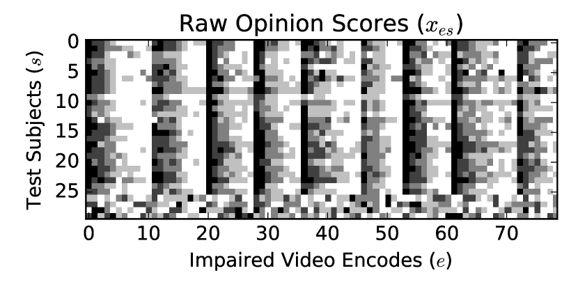
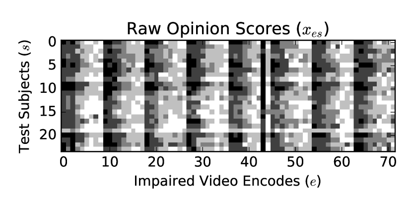
Figure 1: Raw opinion scores from (left) the NFLX dataset and (right) the VQEG dataset. Each pixel represents a raw opinion score. The darker the color, the lower the score. The impaired videos are arranged by contents, and within each content, from low quality to high quality (with the reference video always in the last). For the NFLX dataset, the last four rows correspond to corrupted subjective data.

For many of the experiments, we do not have “ground truth” quality scores to compare against (we only have noisy raw scores). Instead, we use the following methodology in our report of results. For each recovery method, we have a benchmark result, which is the recovered quality scores obtained using that method (for fairness) on an unaltered full dataset. The quality scores recovered under certain conditions (e.g., using a portion of the raw scores, partially corrupted) is compared against the benchmark, and a root-mean-squared-error (RMSE) value is reported. In doing so, we could evaluate, for example, how fast the results converge toward that benchmark result. In other experiments, we do have a “ground truth”, when artificially omitting a subject or creating a corruption on the data.

6.1 An Example

Let us first visually inspect one example result recovered by the MLE and compare it with the MOS. Figure 2 shows the recovered parameters and their corresponding 95% confidence intervals on the full NFLX dataset. Comparing the result with Figure 1 (left), a number of observations can be made:

• The quality scores recovered by MLE are numerically different from the MOS, suggesting that the recovery is non-trivial.

• The confidence intervals for the quality scores recovered by MLE is generally tighter, compared to the ones by MOS, suggesting an estimation with higher confidence.

• Subject #10 has the highest bias, which is evidenced by the whitish horizontal strip visible in Figure 1 (left).

• The last four subjects, whose raw scores were scrambled, have a very high $a_{c}$ value; correspondingly, their estimated bias have very loose confidence interval.

• The content with the highest ambiguity is ElFuente2, which is the “fountain and toddler” scene, known to be difficult to evaluate.

These observations demonstrate the potential of the MLE method on the problem at hand.

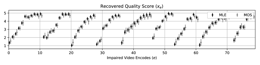
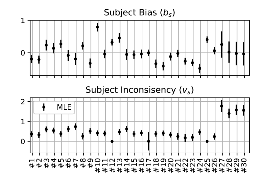
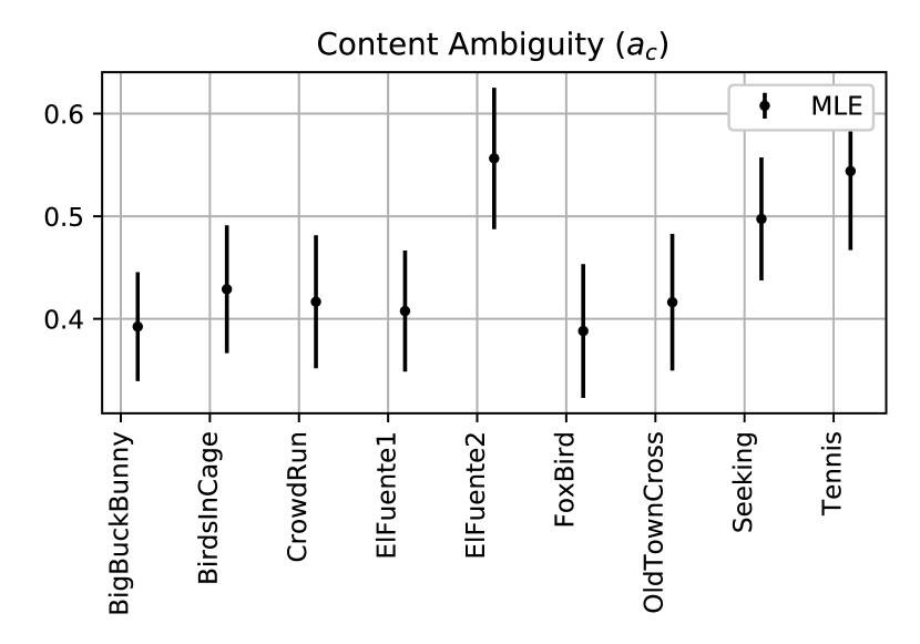
Figure 2: Example recovery result on the NFLX dataset. Both the estimated parameters and their 95% confidence interval are shown.

6.2 Convergence

Next, we evaluate how fast MLE and other methods converge toward the result recovered on the full dataset, as we increase the number of test subjects. For each number of subjects, we randomly sample among all the subjects, and repeated the experiment 100 times. Figure 3 illustrates the averaged RMSE as a function of the subject numbers. It is shown that on the NFLX dataset, MLE has the closest quality scores to the full-dataset recovery than other methods for a given number of subjects. On the VQEG dataset, MLE has performance comparable to MOS and SR-MOS.

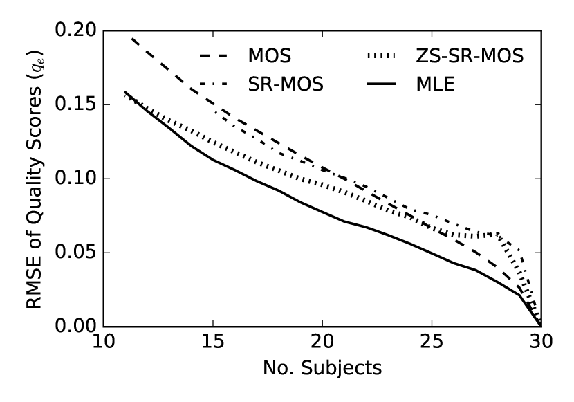
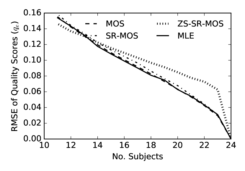
Figure 3: RMSE of the recovered subjective quality scores as a function of the number of test subjects, on (left) the NFLX dataset and (right) the VQEG dataset.

6.3 Resistance to Corruption

From the last section, it is evident that MLE shows faster convergence than other methods in the presence of data scrambling. To further corroborate our speculation, we evaluate how MLE and other methods behave in the presence of data corruption. For each dataset, we simulate two cases of corruption: a) subject corruption, where all the scores corresponding to a number of subjects are scrambled, and b) random corruption, where a raw score gets replaced by a random score from 1 to 5 with a probability. Results for a) and b) are reported in Figure 4 and 5, respectively.

It can be observed that in the presence of subject corruption, MLE achieves a substantial gain over the other methods, including the ones with subject rejection. The reason is that the proposed model was able to capture the variance of subjects explicitly and is able to compensate for it. On the other hand, the traditional subject rejection scheme (Algorithm 1) was only able to identify part of the corrupted subjects. It may also occur that only a subset of a subject’s scores is unreliable. In that case, discarding all of the subject’s scores is a waste of valuable subjective data. Meanwhile, traditional subject rejection employs a set of heuristic steps to determine outliers, which may lack interpretability. By contrast, the proposed model naturally integrates the various subjective effects together and is solved efficiently by our MLE method.

In the presence of random corruption, it can be seen that MLE does not show any advantage over the other methods. This is because the proposed model (1) is incapable of capturing this type of corruption, hence it could not deal with it effectively.

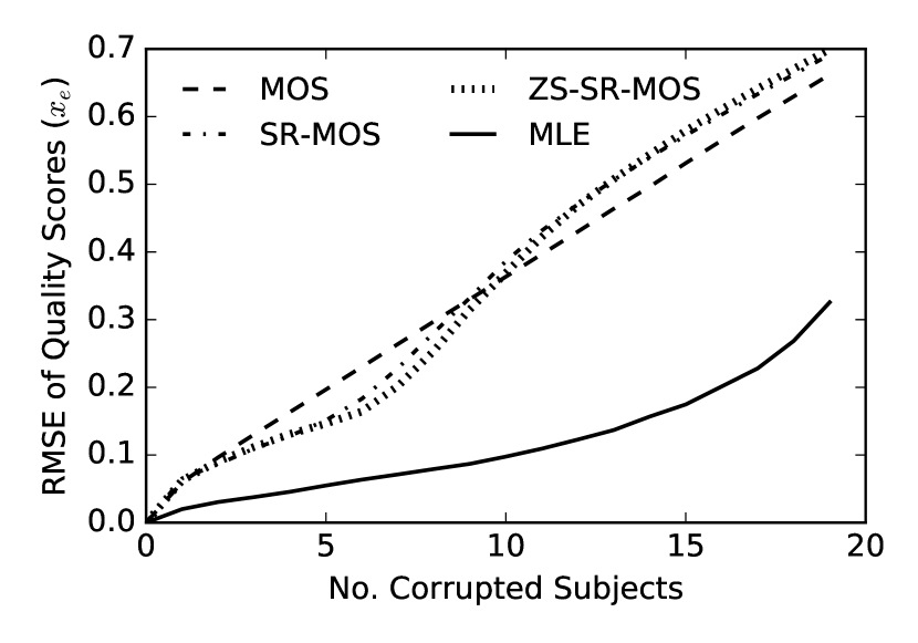
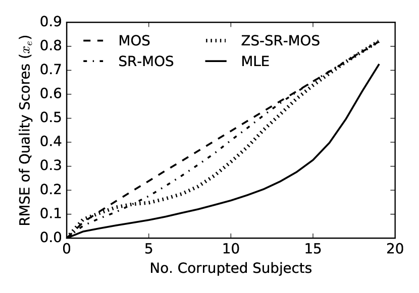
Figure 4: RMSE of the recovered subjective quality scores as a function of the number of corrupted test subjects, on (left) the NFLX dataset and (right) the VQEG dataset.

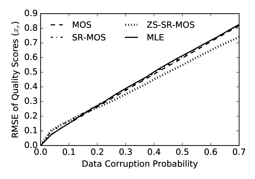
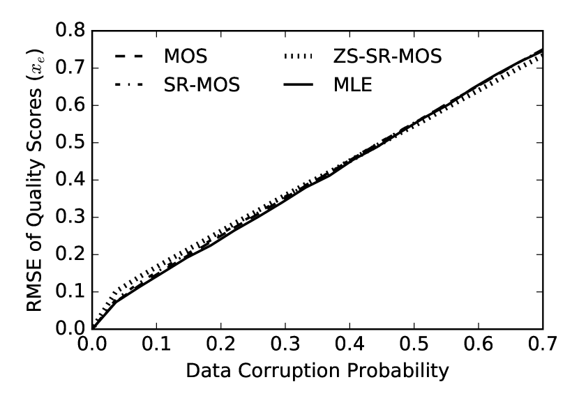
Figure 5: RMSE of the recovered subjective quality scores as a function of the random score corruption probability, on (left) the NFLX dataset and (right) the VQEG dataset.

6.4 Selective Sampling

We also evaluate the MLE and other methods under selective sampling, where each subject only rates a part of all videos. We performed this step by assigning each raw score a random probability of presence. As the probability increases, more scores are sampled. The performance is reported in Figure 6. On the NFLX dataset, again, MLE has clear advantage over other methods. On the VQEG dataset, MLE also shows gain over other methods. Since MLE accounts for the full information, randomly missing some data points does not affect its predictive performance by much. By contrast, the MOS, SR-MOS, ZS-SR-MOS methods, which make local decisions on partial information, are greatly affected.

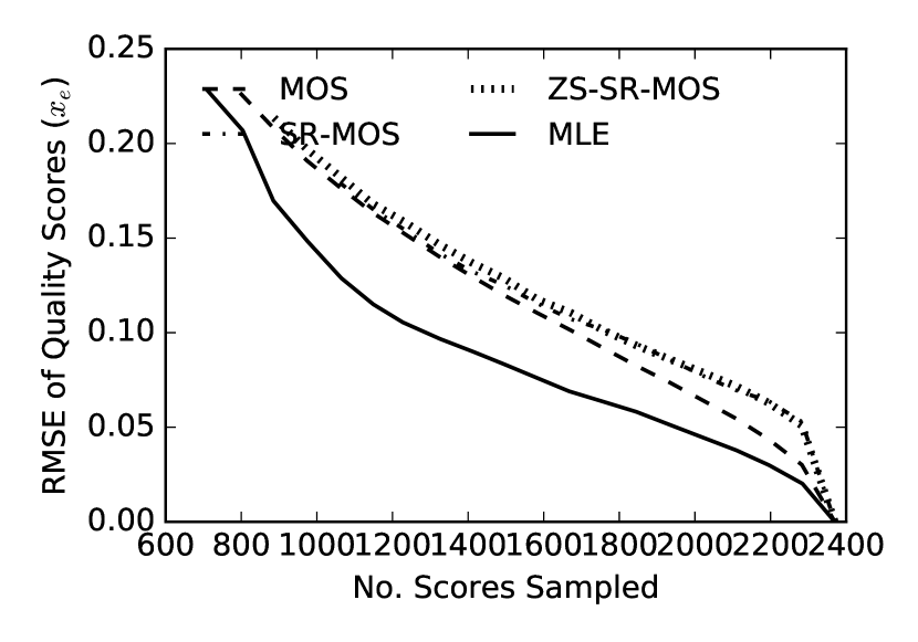
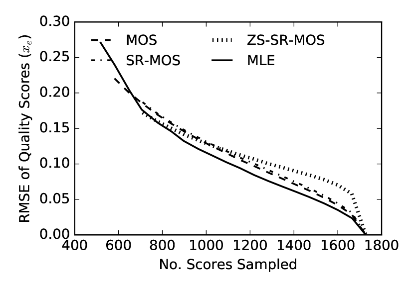
Figure 6: RMSE of the recovered subjective quality scores as a function of the number of scores randomly sampled, on (left) the NFLX dataset and (right) the VQEG dataset.

7 Summary and Future Work

We have presented a new approach to process raw opinion scores collected in video quality subjective testing, by using a generative model that jointly captures the quality of impaired videos, bias and inconsistency of subjects and the ambiguity of contents. We determined the model parameters by formulating a MLE problem and devising a belief propagation solution. It was shown that the recovered parameters were able to capture the subjective effects (bias, inconsistencies etc.) of the problem at hand, and that the proposed solution outperformed other methods in terms of its resistance to subject corruption, tighter confidence interval, better handling of missing data and provision of side information on the test subjects and video contents.

We list a number of directions to further this work: 1) The recovered side information on the test subjects and video contents can be used actively in the process to train an objective quality metric to yield more accurate prediction. 2) The proposed model can be further extended to other test methods, such as pairwise comparison. 3) A theoretical analysis on the belief propagation algorithm can uncover its region of convergence.

8 References

Appendix A Analysis of Z-score Transformation

Let us assume a simplified version of model (1):

$$X_{e,s} = x_{e}+B_{e,s}$$

$$B_{e,s} \sim \mathcal{N}(b_{s},v_{s}^{2}).$$

Let $y_{e,s}=x_{e,s}-\mu_{s}$ be the mean-subtracted version of $x_{e,s}$, and let $B_{e,s}=b_{s}+v_{s}N_{e,s}$ where $N_{e,s}\sim\mathcal{N}(0,1)$. The corresponding random variable $Y_{e,s}$ has the form:

$$Y_{e,s} = X_{e,s}-\frac{1}{E}\sum_{e^{\prime}}X_{e^{\prime},s}$$ (5)

$$= x_{e}+b_{s}+v_{s}N_{e,s}-\frac{1}{E}\sum_{e^{\prime}}(x_{e^{\prime}}+b_{s}+v_{s}N_{e^{\prime}s})$$

$$= (x_{e}-\frac{1}{E}\sum_{e^{\prime}}x_{e^{\prime}})+v_{s}N_{e,s}-\frac{1}{E}v_{s}\sum_{e^{\prime}}N_{e^{\prime}s}$$

$$= y_{e}+\frac{E-1}{E}v_{s}N_{e,s}-\frac{1}{E}v_{s}\sum_{e^{\prime}:e^{\prime}\neq e}N_{e^{\prime}s}$$

$$\simeq y_{e}+v_{s}N_{e,s},$$ (6)

where in (5) we define $y_{e}=x_{e}-\mu_{x}$ and $\mu_{x}=\frac{1}{E}\sum_{e^{\prime}}x_{e^{\prime}}$, and (6) is due to $E\gg 1$. Z-score transformation computes the z-score $z_{e,s}=(x_{e,s}-\mu_{s})\left/\sigma_{s}\right.=y_{e,s}\left/\sqrt{\frac{1}{E}\sum_{e^{\prime}}y_{e^{\prime},s}^{2}}\right.$. The corresponding random variable $Z_{e,s}$ has the form:

$$Z_{e,s} = \frac{Y_{e,s}}{\sqrt{\frac{1}{E}\sum_{e^{\prime}}Y_{e^{\prime},s}^{2}}}$$ (7)

$$\simeq \frac{y_{e}+v_{s}N_{e,s}}{\sqrt{\frac{1}{E}\sum_{e^{\prime}}(y_{e^{\prime}}+v_{s}N_{e^{\prime},s})^{2}}}$$

$$\simeq \frac{y_{e}+v_{s}N_{e,s}}{\sqrt{\frac{1}{E}\sum_{e^{\prime}}y_{e^{\prime}}{}^{2}+\frac{1}{E}v_{s}^{2}\sum_{e^{\prime}}N_{e^{\prime},s}^{2}}}$$

$$= \frac{x_{e}-\mu_{x}+v_{s}N_{e,s}}{\sqrt{\sigma_{x}^{2}+\frac{1}{E}v_{s}^{2}\sum_{e^{\prime}}N_{e^{\prime},s}^{2}}}$$

$$\neq \frac{x_{e}-\mu_{x}}{\sigma_{x}},$$

where (7) is due to that $\sum_{e}y_{e}=0$ and in (A) we define $\sigma_{x}=\sqrt{\frac{1}{E}\sum_{e}y_{e}^{2}}$. The last inequality suggests that there are non-vanishing terms related to subjects that cannot be canceled out by z-score transformation. In other words, z-scoring can only partially compensate subjects’ bias and inconsistency.

Appendix B Analysis of Observations and Unknowns in (1)

We consider the observations and unknowns in (1). Assume a typical scenario, where the subjective experiment has $S=30$ subjects, $C=20$ contents, and $E=200$ impaired videos. The number of unknowns is thus $E+2S+C=280$ and the number of observations is $ES=6000$. At a first glance, we may conclude that the number of observations are much greater than the number of unknowns, and the problem has a well-conditioned solution.

Sounds pretty good? Let’s take a closer look. This time, consider a simplified model by removing the variation terms $\{v_{s}\}$ and $\{a_{c}\}$, i.e.,

$$x_{e,s}=x_{e}+b_{s}.$$

After the variation terms are removed, everything is deterministic. Since the relationship is linear, we hope to find a least-squares solution of a linear system with $ES$ observations and $E+S$ unknowns. Let $u=[\{x_{e}\}_{e=1}^{E},\{b_{s}\}_{s=1}^{S}]{}^{T}$ be the vector of unknowns, and $o=[\{x_{e,s}\}]{}^{T}$ be the vector of observations, and let $\Omega=[\Omega_{i,j}]$ be a $ES\times(E+S)$ matrix, where $\Omega_{e+(s-1)E,e}=1$ and $\Omega_{e+(s-1)E,s+E}=1$ for $e=1,...,E$ and $s=1,...,S$, and the rest of the elements are all zeros. We look to find a least-squares solution to the following linear system:

$$\Omega\cdot u=o.$$

Proposition 1.

Matrix $\Omega$ has rank $E+S-1$.

Proof.

Apply Gaussian elimination. The first $E$ rows are independent. Subtract the $(e+(s-1)E)$-th row by the $e$-th row, $e=1,...,E$ and $s=1,..,S$, we can get another $(S-1)$ independent rows. In total, there are $E+S-1$ independent rows in $\Omega$. ∎

Proposition 1 implies that we are missing one equation, and without it there are infinite number of solutions. Fortunately, it is not too difficult to come up with one additional equation that is reasonable. For example, we can let the first impaired video have a score equal to its MOS, i.e.,

$$x_{e=1}=\mu_{e=1}.$$

We can readily find the least-squares solution after adding the additional condition, which is also necessary for solving the full model (1).

Appendix C Derivation of Update Rules in Algorithm 2

This section derives the update rules used in Algorithm 2. Consider $L(\theta)$ derived in (3) where $\theta=(\{x_{e}\},\{b_{s}\},\{v_{s}\},\{a_{c}\})$. The first-order partial derivatives of $L(\theta)$ are expressed as follows:

$$\frac{\partial L(\theta)}{\partial x_{e}} = \sum_{s}\frac{x_{e,s}-x_{e}-b_{s}}{v_{s}^{2}+a_{\mathsf{c}(e)}^{2}}$$

$$\frac{\partial L(\theta)}{\partial b_{s}} = \sum_{e}\frac{x_{e,s}-x_{e}-b_{s}}{v_{s}^{2}+a_{\mathsf{c}(e)}^{2}}$$

$$\frac{\partial L(\theta)}{\partial v_{s}} = \sum_{e}-\frac{v_{s}}{v_{s}^{2}+a_{\mathsf{c}(e)}^{2}}+\frac{v_{s}(x_{e,s}-x_{e}-b_{s})^{2}}{\left(v_{s}^{2}+a_{\mathsf{c}(e)}^{2}\right)^{2}}$$

$$\frac{\partial L(\theta)}{\partial a_{c}} = \sum_{s,e:\mathsf{c}(e)=c}-\frac{a_{\mathsf{c}(e)}}{v_{s}^{2}+a_{\mathsf{c}(e)}^{2}}+\frac{a_{\mathsf{c}(e)}(x_{e,s}-x_{e}-b_{s})^{2}}{\left(v_{s}^{2}+a_{\mathsf{c}(e)}^{2}\right)^{2}}$$

Repeat the differentiation and we get the second-order partial derivatives:

$$\frac{\partial^{2}L(\theta)}{\partial x_{e}^{2}} = \sum_{s}-\frac{1}{v_{s}^{2}+a_{\mathsf{c}(e)}^{2}}$$ (9)

$$\frac{\partial^{2}L(\theta)}{\partial b_{s}^{2}} = \sum_{e}-\frac{1}{v_{s}^{2}+a_{\mathsf{c}(e)}^{2}}$$ (10)

$$\frac{\partial^{2}L(\theta)}{\partial v_{s}^{2}} = \sum_{e}-\frac{a_{\mathsf{c}(e)}^{2}-v_{s}^{2}}{\left(v_{s}^{2}+a_{\mathsf{c}(e)}^{2}\right)^{2}}+\frac{(x_{e,s}-x_{e}-b_{s})^{2}\left(a_{\mathsf{c}(e)}^{4}-2a_{\mathsf{c}(e)}^{2}v_{s}^{2}-3v_{s}^{4}\right)}{\left(v_{s}^{2}+a_{\mathsf{c}(e)}^{2}\right)^{4}}$$ (11)

$$\frac{\partial^{2}L(\theta)}{\partial a_{c}^{2}} = \sum_{s,e:\mathsf{c}(e)=c}-\frac{v_{s}^{2}-a_{\mathsf{c}(e)}^{2}}{\left(v_{s}^{2}+a_{\mathsf{c}(e)}^{2}\right)^{2}}+\frac{(x_{e,s}-x_{e}-b_{s})^{2}\left(v_{s}^{4}-2v_{s}^{2}a_{\mathsf{c}(e)}^{2}-3a_{\mathsf{c}(e)}^{4}\right)}{\left(v_{s}^{2}+a_{\mathsf{c}(e)}^{2}\right)^{4}}$$ (12)

Define $w_{e,s}=\frac{1}{v_{s}^{2}+a_{\mathsf{c}(e)}^{2}}$. Applying the expressions above to the Newton-Raphson update rules yield:

$$x_{e}^{new} = \frac{\sum_{s}w_{e,s}(x_{e,s}-b_{s})}{\sum_{s}w_{e,s}}$$

$$b_{s}^{new} = \frac{\sum_{e}w_{e,s}(x_{e,s}-x_{e})}{\sum_{e}w_{e,s}}$$

$$v_{s}^{new} v_{s}-\frac{\sum_{e}w_{e,s}v_{s}-w_{e,s}^{2}v_{s}(x_{e,s}-x_{e}-b_{s})^{2}}{\sum_{e}w_{e,s}^{2}(a_{\mathsf{c}(e)}^{2}-v_{s}^{2})-w_{e,s}^{4}(x_{e,s}-x_{e}-b_{s})^{2}\left(a_{\mathsf{c}(e)}^{4}-2a_{\mathsf{c}(e)}^{2}v_{s}^{2}-3v_{s}^{4}\right)}$$ =

$$a_{c}^{new} = a_{c}-\frac{\sum_{s,e:\mathsf{c}(e)=c}w_{e,s}a_{\mathsf{c}(e)}-w_{e,s}^{2}a_{\mathsf{c}(e)}(x_{e,s}-x_{e}-b_{s})^{2}}{\sum_{s,e:\mathsf{c}(e)=c}w_{e,s}^{2}(v_{s}^{2}-a_{\mathsf{c}(e)}^{2})-w_{e,s}^{4}(x_{e,s}-x_{e}-b_{s})^{2}\left(v_{s}^{4}-2v_{s}^{2}a_{\mathsf{c}(e)}^{2}-3a_{\mathsf{c}(e)}^{4}\right)}$$

Note that there is strong intuition behind the expressions for $x_{e}^{new}$ and $b_{s}^{new}$. In each iteration, $x_{e}^{new}$ is re-estimated, by the sum of opinion scores $x_{e,s}$ with the currently estimated bias $b_{s}$ removed. Each opinion score is weighted by $w_{e,s}$, i.e., the higher the variance (subject inconsistency and content ambiguity), the less reliable the opinion score, hence less the weight. We can interpret $b_{s}^{new}$ in a similar way.

Appendix D Derivation of Confidence Interval (4)

Let $I(\theta)$ be the Fisher information of parameter $\theta$ defined by

$$I(\theta)=E\left[\left(\frac{\partial L(\theta)}{\partial\theta}\right)^{2}\right]=-E\left[\frac{\partial^{2}L(\theta)}{\partial\theta^{2}}\right]$$

where the second equation is true if $L(\theta)$ is twice-differentiable and $E\left[\frac{\partial L(\theta)}{\partial\theta}\right]=0$. The Cramer-Rao bound states that the variance of $\hat{\theta}$ is lower-bounded by the reciprocal of $I(\theta)$:

$$\operatorname{var}(\hat{\theta})\geq\frac{1}{I(\theta)},$$

where the equality holds for the Gaussian case. Using the Gaussian assumption and observed Fisher information, we have $\operatorname{var}(\hat{\theta})=\frac{1}{-\frac{\partial^{2}L(\theta)}{\partial\theta^{2}}}$. Substituting into the 95% confidence interval $\hat{\theta}\pm 1.96\operatorname{std}(\hat{\theta})$, we have (4).

References

- [1] Z. Wang, A. C. Bovik, H. R. Sheikh, and E. P. Simoncelli, “Image quality assessment: from error visibility to structural similarity,” IEEE Transactions on Image Processing, vol. 13, no. 4, pp. 600–612, April 2004.
- [2] A. Aaron, Z. Li, M. Manohara, J. D. Cock, and D. Ronca. Per-Title Encode Optimization. [Online]. Available: http://techblog.netflix.com/2015/12/per-title-encode-optimization.html
- [3] Z. Li, A. Aaron, I. Katsavounidis, A. Moorthy, and M. Manohara. Toward A Practical Perceptual Video Quality Metric. [Online]. Available: http://techblog.netflix.com/2016/06/toward-practical-perceptual-video.html
- [4] J. Y. Lin, T.-J. Liu, E. C.-H. Wu, and C.-C. J. Kuo, “A Fusion-based Video Quality Assessment (FVQA) Index,” APSIPA Trans. Signal and Information Processing, 2014.
- [5] S. Wolf and M. H. Pinson, “Video Quality Model for Variable Frame Delay (VQM-VFD),” Nat. Telecommun. Inf. Admin., Tech. Memo, TM-11-482, Sep. 2011.
- [6] C.Cortes and V.Vapnik, “Support-Vector Networks,” Machine Learning, vol. 20, no. 3, pp. 273–297, 1995.
- [7] K. Seshadrinathan, R. Soundararajan, A. C. Bovik, and L. K. Cormack, “Study of subjective and objective quality assessment of video,” IEEE Transactions on Image Processing, vol. 19, no. 6, pp. 1427–1441, June 2010.
- [8] ITU-R BT.500: Methodology for the Subjective Assessment of the Quality of Television Pictures. [Online]. Available: https://www.itu.int/rec/R-REC-BT.500
- [9] D. J. C. MacKay, Information Theory, Inference, and Learning Algorithms. Cambridge University Press, 2003.
- [10] T. Cover and J. Thomas, Elements of Information Theory, ser. A Wiley-Interscience publication. Wiley, 2006.
- [11] VMAF Open-Source Project. [Online]. Available: https://github.com/Netflix/vmaf
- [12] ITU-T P.910: Subjective Video Quality Assessment Methods for Multimedia Applications. [Online]. Available: https://www.itu.int/rec/T-REC-P.910
- [13] L. Janowski and M. Pinson, “The accuracy of subjects in a quality experiment: A theoretical subject model,” IEEE Transactions on Multimedia, vol. 17, no. 12, pp. 2210–2224, Dec 2015.
- [14] J. Whitehill, T. fan Wu, J. Bergsma, J. R. Movellan, and P. L. Ruvolo, “Whose vote should count more: Optimal integration of labels from labelers of unknown expertise,” in Advances in Neural Information Processing Systems, 2009, pp. 2035–2043.
- [15] W. Wang, J. Allebach, and Y. Guo, “Image quality evaluation using image quality ruler and graphical model,” in IEEE Int. Conf. Image Processing (ICIP), 2015.
- [16] Netflix Public Dataset. [Online]. Available: https://github.com/Netflix/vmaf#netflix-public-dataset
- [17] “Report on the Validation of Video Quality Models for High Definition Video Content,” Video Quality Experts Group (VQEG), Tech. Rep., Version 2.0, June 30, 2010.