Causes for Query Answers from Databases: Datalog Abduction, View-Updates, and Integrity Constraints

Abstract

Causality has been recently introduced in databases, to model, characterize, and possibly compute causes for query answers. Connections between QA-causality and consistency-based diagnosis and database repairs (wrt. integrity constraint violations) have already been established. In this work we establish precise connections between QA-causality and both abductive diagnosis and the view-update problem in databases, allowing us to obtain new algorithmic and complexity results for QA-causality. We also obtain new results on the complexity of view-conditioned causality, and investigate the notion of QA-causality in the presence of integrity constraints, obtaining complexity results from a connection with view-conditioned causality. The abduction connection under integrity constraints allows us to obtain algorithmic tools for QA-causality.

1 Introduction

Causality is an important concept that appears at the foundations of many scientific disciplines, in the practice of technology, and also in our everyday life. Causality is fundamental to understand and manage uncertainty in data, information, knowledge, and theories. In data management in particular, there is a need to represent, characterize and compute causes that explain why certain query results are obtained or not, or why natural semantic conditions, such as integrity constraints, are satisfied or not. Causality can also be used to explain the contents of a view, i.e. of a predicate with virtual contents that is defined in terms of other physical, materialized relations (tables).

Most of the work on causality has been developed in the context of artificial intelligence [50] and Statistics [51], and little has been said about causality in data management. In this work we concentrate on causality as defined for- and applied to relational databases. In a world of big, uncertain data, the necessity to understand the data beyond direct query answers, introducing explanations in different forms, becomes particularly relevant.

The notion of causality-based explanation for a query result was introduced in [47], on the basis of the deeper concept of actual causation. We will refer to this notion as query-answer causality (or simply, QA-causality). Intuitively, a database atom (or tuple) $\tau$  is an actual cause for an answer $\bar{a}$ to a conjunctive query $\mathcal{Q}$ from a relational instance $D$ if there is a “contingent” subset of tuples $\Gamma$, accompanying $\tau$, such that, after removing $\Gamma$ from $D$, removing $\tau$ from $D\smallsetminus\Gamma$ causes $\bar{a}$ to switch from being an answer to being a non-answer (i.e. not being an answer). Usually, actual causes and contingent tuples are restricted to be among a pre-specified set of endogenous tuples, which are admissible, possible candidates for causes, as opposed to exogenous tuples.

A cause $\tau$ may have different associated contingency sets $\Gamma$. Intuitively, the smaller they are the strongest is $\tau$ as a cause (it need less company to undermine the query answer). So, some causes may be stronger than others. This idea is formally captured through the notion of causal responsibility, and introduced in [47]. It reflects the relative degree of actual causality. In applications involving large data sets, it is crucial to rank potential causes according to their responsibilities [48, 47].

Furthermore, view-conditioned causality (in short, vc-causality) was proposed in [48, 49] as a restricted form of QA-causality, to determine causes for unexpected query results, but conditioned to the correctness of prior knowledge that cannot be altered by hypothetical tuple deletions.

Actual causation, as used in [47, 48, 49], can be traced back to [33], which provides a model-based account of causation on the basis of counterfactual dependence. Causal responsibility was introduced in [15], to provide a graded, quantitative notion of causality when multiple causes may over-determine an outcome.

In [59, 7] connections were established between QA-causality and database repairs [4], which allowed to obtain several complexity results for QA-causality related problems. Connections between QA-causality and consistency-based diagnosis [56] were established in [59, 7]. More specifically, QA-causality and causal responsibility were characterized in terms of consistency-based diagnosis, which led to new algorithmic results for QA-causality [59, 7]. In [6] first connections between QA-causality, view updates, and abductive diagnosis in Datalog [19, 25] were announced. We elaborate on this in the rest of this section.

The definition of QA-causality applies to monotone queries [47, 48]. However, all complexity and algorithmic results in [47, 59] have been restricted to first-order (FO) monotone queries, mainly conjunctive queries. However, Datalog queries [13, 1], which are also monotone, but may contain recursion, require investigation in the context of QA-causality.

In contrast to consistency-based diagnoses, which is usually practiced with FO specifications, abductive diagnosis is commonly done with different sorts of logic programming-based specifications [24, 26, 32]. In particular, Datalog can be used as the specification language, giving rise to Datalog-abduction [32]. In this work we establish a relationship between Datalog-abduction and QA-causality, which allows us to obtain complexity results for QA-causality for Datalog queries.

We also explore fruitful connections between QA-causality and the classical and important view-update problem in databases [1], which is about updating a database through views. An important aspect of the problem is that one wants the base relations (sometimes called “the source database”) to change in a minimal way while still producing the intended view updates. This is an update propagation problem, from views to base relations.

The delete-propagation problem [12, 42, 43] is a particular case of the view-update problem, where only tuple deletions are allowed from the views. If the views are defined by monotone queries, only source deletions can give an account of view deletions. When only a subset-minimal set of deletions from the base relations is expected to be performed, we are in the “minimal source-side-effect” case. The “minimum source-side-effect” case appears when that set is required to have a minimum cardinality. In a different case, we may want to minimize the side-effects on the view, requiring that other tuples in the (virtual) view contents are not affected (deleted) [12].

In this work we provide precise connections between QA-causality and different variants of the delete-propagation problem. In particular, we show that the minimal-source-side-effect deletion-problem and the minimum-source-side-effect deletion-problem are related to QA-causality for monotone queries and the most-responsible cause problem, as investigated in [47, 59, 7]. The minimum-view-side-effect deletion-problem is related to vc-causality. We establish precise mutual characterizations (reductions) between these problems, obtaining in particular, new complexity results for view-conditioned causality.

Finally, we also define and investigate the notion of query-answer causality in the presence of integrity constraints, which are logical dependencies between database tuples [1]. Under the assumption that the instance at hand satisfies a given set of ICs, the latter should have an effect on the causes for a query answer, and their computation. We show that they do, proposing a notion of QA-cause under ICs. But taking advantage of the connection with Datalog-abduction (this time under ICs on the extensional relations), we develop techniques to compute causes for query answers from Datalog queries in the presence of ICs.

Summarizing, our main results are the following:

1. We establish precise connections between QA-causality for Datalog queries and abductive diagnosis from Datalog specifications, i.e. mutual characterizations and computational reductions between them.

2. We establich that, in contrast to (unions of) conjunctive queries, deciding tuple causality for Datalog queries is NP-complete in data.

3. We identify a class of (possibly recursive) Datalog queries for which deciding causality is fixed-parameter tractable in combined complexity.

4. We establish that deciding whether the causal responsibility of a tuple for a Datalog query-answer is greater than a given threshold is NP-complete in data.

5. We establish mutual characterizations between QA-causality and different forms of delete-propagation as a view-update problem.

6. We obtain that computing the size of the solution to a minimum-source-side-effect deletion-problem is hard for the complexity class ${\it FP}^{\it NP(log(n))}$, that of computational problems solvable in polynomial time (in data) by calling a logarithmic number of times an NP-oracle.

7. We investigate in detail the problem of view-conditioned QA-causality (vc-causality), and we establish connections with the view-side-effect free delete propagation problem for view updates.

8. We obtain that deciding if an answer has a vc-cause is NP-complete in data; that deciding tuple vc-causality is NP-complete in data; and deciding if the vc-causal responsibility of a tuple for a Datalog query-answer is greater than a given threshold is also NP-complete in data.

9. We define the notion of QA-causality in the presence of integrity constraints (ICs), and investigate its properties. In particular, we make the case that the new property provides natural results.

10. We obtain complexity results for QA-causality under ICs. In particular, we show that even for conjunctive queries, deciding tuple causality may become NP-hard under inclusion dependencies.

11. We establish connections between QA-causality for Datalog queries under ICs and the view update problem and abduction from Datalog specifications, both under ICs. Through these connections we provide algorithmic results for computing causes for Datalog query answers under ICs.

This paper is structured as follows. Section 2 provides background material on relational databases and Datalog queries. Section 3 introduces the necessary concepts, known results, and the main computational problems for QA-causality. Section 4 introduces the abduction problem in Datlog specifications, and establishes its connections with QA-causality. Section 5 introduces the main problems related to updates trough views defined by monotone queries, and their connections with QA-causality problems. Section 6 defines and investigates view-conditioned QA-causality. Section 7 defines and investigates QA-causality under integrity constraints. Finally, Section 8 discusses some relevant related problems and draws final conclusions. The Appendix contains a couple of proofs that are not in the main body of the paper. This paper is an extension of both [60] and [62].

2 Preliminaries

We consider relational database schemas of the form $\mathcal{S}=(U,\mathcal{P})$, where $U$ is the possibly infinite database domain and $\mathcal{P}$ is a finite set of database predicates of fixed arities. A database instance $D$ compatible with $\mathcal{S}$ can be seen as a finite set of ground atomic formulas (a.k.a. atoms or tuples), of the form $P(c_{1},...,c_{n})$, where $P\in\mathcal{P}$ has arity $n$, and $c_{1},\ldots,c_{n}\in U$.

A conjunctive query (CQ) is a formula of the first-order (FO) language $\mathcal{L}(\mathcal{S})$ associated to $\mathcal{S}$, of the form  $\mathcal{Q}(\bar{x})\!:\exists\bar{y}(P_{1}(\bar{s}_{1})\wedge\cdots\wedge P_{m}(\bar{s}_{m}))$, where the $P_{i}(\bar{s}_{i})$ are atomic formulas, i.e. $P_{i}\in\mathcal{P}$, and the $\bar{s}_{i}$ are sequences of terms, i.e. variables or constants of $U$. The $\bar{x}$ in $\mathcal{Q}(\bar{x})$ shows all the free variables in the formula, i.e. those not appearing in $\bar{y}$. A sequence $\bar{c}$ of constants is an answer to query $\mathcal{Q}(\bar{x})$ if $D\models\mathcal{Q}[\bar{c}]$, i.e. the query becomes true in $D$ when the free variables are replaced by the corresponding constants in $\bar{c}$. We denote the set of all answers from instance $D$ to a conjunctive query $\mathcal{Q}(\bar{x})$ with $\mathcal{Q}(D)$.

A conjunctive query is Boolean (a BCQ), if $\bar{x}$ is empty, i.e. the query is a sentence, in which case, it is true or false in $D$, denoted by $D\models\mathcal{Q}$ and $D\not\models\mathcal{Q}$, respectively. Accordingly, when $\mathcal{Q}$ is a BCQ, $\mathcal{Q}(D)=\{{\it yes}\}$ if $\mathcal{Q}$ is true, and $\mathcal{Q}(D)=\emptyset$, otherwise.

A query $\mathcal{Q}$ is monotone if for every two instances $D_{1}\subseteq D_{2}$,  $\mathcal{Q}(D_{1})\subseteq\mathcal{Q}(D_{2})$, i.e. the set of answers grows monotonically with the instance. For example, CQs and unions of CQs (UCQs) are monotone queries. In this work we consider only monotone queries.

An integrity constraint (IC) is a sentence $\varphi$ in the language $\mathcal{L}(\mathcal{S})$. For a given instance $D$ for schema $\mathcal{S}$, it may be true or false in $D$, which is denoted with $D\models\varphi$, resp. $D\not\models\varphi$. Given a set $\Sigma$ of integrity constraints, a database instance $D$ is consistent if $D\models\Sigma$; otherwise it is said to be inconsistent. In this work we assume that sets of integrity constraints are always finite and logically consistent (i.e. they are all simultaneously true in some instance).

A particular class of ICs is formed by inclusion dependencies (INDs), which are sentences of the form $\forall\bar{x}(P(\bar{x})\rightarrow\exists\bar{y}R(\bar{x}^{\prime},\bar{y}))$, with $P,R$ predicates, $\bar{x}^{\prime}\cap\bar{y}=\emptyset$, and $\bar{x}^{\prime}\subseteq\bar{x}$. The tuple-generating dependencies (tgds) are ICs that generalize INDs, and are of the form  $\forall\bar{x}(\bigwedge_{i}P_{i}(\bar{x}_{i})\rightarrow\exists\bar{y}\bigwedge_{j}P_{j}(\bar{x}_{j}^{\prime},\bar{y}_{j}))$, with $P_{i},P_{j}$ predicates, $\bar{x}_{j}^{\prime}\subseteq\bigcup\bar{x}_{i}=\bar{x}$, and $\bar{y}_{j}\cap\bar{x}=\emptyset$.

Another special class of ICs is formed by functional dependencies (FDs). For example, $\psi\!:\forall x\forall y\forall z(P(x,y)\land P(x,z)\rightarrow y=z)$ specifies that the second attribute of $P$ functionally depends upon the first. (If $A,B$ are the first and second attributes for $P$, the usual notation for this FD is  $P\!:\ A\rightarrow B$.) Actually, this FD is also a key constraint (KC), in the sense that the attribute(s) on the LHS of the arrow functionally determines all the other attributes of the predicate. FDs form a particular class of equality-generating dependencies (egds), which are ICs of the form  $\forall\bar{x}(\bigwedge_{i}P_{i}(\bar{x}_{i})\rightarrow x_{j}=x_{k}))$, with $x_{j},x_{k}\in\bar{x}$ (cf. [1] for more details on ICs).

Given a relational schema $\mathcal{S}$, queries $\mathcal{Q}_{1}(\bar{x}),\mathcal{Q}_{2}(\bar{x})$, and a set $\Sigma$ of ICs (all for schema schema $\mathcal{S}$), $\mathcal{Q}_{1}$ and $\mathcal{Q}_{2}$ are equivalent wrt. $\Sigma$, denoted $\mathcal{Q}_{1}\equiv_{\Sigma}\mathcal{Q}_{2}$, iff $\mathcal{Q}_{1}(D)=\mathcal{Q}_{2}(D)$ for every instance $D$ for $\mathcal{S}$ that satisfies $\Sigma$. One can define in similar terms the notion of query containment under ICs, denoted $\mathcal{Q}_{1}\subseteq_{\Sigma}\mathcal{Q}_{2}$.

A Datalog query $\mathcal{Q}(\bar{x})$ is a whole program $\Pi$ consisting of positive Horn rules (a.k.a. positive definite rules), of the form  $P(\bar{t})\leftarrow P_{1}(\bar{t}_{1}),\ldots,P_{n}(\bar{t}_{n})$, with the $P_{i}(\bar{t}_{i})$ atomic formulas. All the variables in $\bar{t}$ appear in some of the $\bar{t}_{i}$. Here, $n\geq 0$, and if $n=0$, $P(\bar{t})$ is called a fact and does not contain variables. We assume the facts are those stored in an underlying extensional database $D$.

We may assume that a Datalog program $\Pi$ as a query defines an answer-collecting predicate ${\it Ans}(\bar{x})$ by means of a top rule of the form ${\it Ans}(\bar{t})\leftarrow P_{1}(\bar{t}_{1}),\ldots,P_{m}(\bar{t}_{m})$, where all the predicates in the RHS (a.k.a. as the rule body) are defined by other rules in $\Pi$ or are database predicates for $D$. Here, the $\bar{t},\bar{t}_{i}$ are lists of variables or constants, and the variables in $\bar{t}$ belong to $\bigcup_{i}\bar{t}_{i}$.

Now, $\bar{a}$ is an answer to query $\Pi$ on $D$ when $\Pi\cup D\models{\it Ans}(\bar{a})$. Here, entailment ($\models$) means that the RHS belongs to the minimal model of the LHS. So, the extension, ${\it Ans}(\Pi\cup D)$, of predicate ${\it Ans}$ contains the answers to the query in the minimal model of the program (including the database). The Datalog query is Boolean if the top answer-predicate is propositional, with a definition of the form ${\it ans}\leftarrow P_{1}(\bar{s}_{1}),\ldots,P_{m}(\bar{s}_{m})$. In this case, the query is true if $\Pi\cup D\models{\it ans}$, equivalently, if ${\it ans}$ belongs to the minimal model of $\Pi\cup D$  [1, 13].

Datalog queries may contain recursion, and then they may not be FO [1, 13]. However they are also monotone.

3 QA-Causality and its Decision Problems

In this section we review the notion of QA-causality as introduced in [47]. We also summarize the main decision and computational problems that emerge in this context and the established results for them.

3.1 Causality and responsibility

In the rest of this work, unless otherwise stated, we assume that a relational database instance $D$ is split in two disjoint sets, $D=D^{n}\cup D^{x}$, where $D^{n}$ and $D^{x}$ are the sets of endogenous and exogenous tuples, respectively. The former are tuples that we may consider as potential causes for data phenomena, tuples on which we have some form of control and can assess and modify. The latter are supposed to be given, unquestioned, and as such, not considered as possible causes. For example, they could be tuples provided by external sources we have no control upon.

A tuple $\tau\in D^{n}$ is a counterfactual cause for an answer $\bar{a}$ to $\mathcal{Q}(\bar{x})$ in $D$ if $D\models\mathcal{Q}(\bar{a})$, but $D\smallsetminus\{\tau\}\not\models\mathcal{Q}(\bar{a})$. A tuple $\tau\in D^{n}$ is an actual cause for $\bar{a}$ if there exists $\Gamma\subseteq D^{n}$, called a contingency set, such that $\tau$ is a counterfactual cause for $\bar{a}$ in $D\smallsetminus\Gamma$. ${\it Causes}(D,\mathcal{Q}(\bar{a}))$ denotes the set of actual causes for $\bar{a}$. If $\mathcal{Q}$ is Boolean, ${\it Causes}(D,\mathcal{Q})$ contains the causes for answer ${\it yes}$. For $\tau\in{\it Causes}(D,\mathcal{Q}(\bar{a}))$,  ${\it Cont}(D,\mathcal{Q}(\bar{a}),\tau)$ denotes the set of contingency sets for $\tau$ as a cause for $\mathcal{Q}(\bar{a})$ in $D$.

Notice that ${\it Causes}(D,\mathcal{Q}(\bar{a}))$ is non-empty when $D\models\mathcal{Q}(\bar{a})$, but $D^{x}\not\models\mathcal{Q}(\bar{a})$, reflecting the fact that endogenous tuples are required for the answer.

Given a $\tau\in{\it Causes}(D,\mathcal{Q}(\bar{a}))$, we collect all subset-minimal contingency sets associated with $\tau$:

$${{\it Cont}^{s}(D,\mathcal{Q}(\bar{a}),\tau)} := \{\Gamma\subseteq D^{n}~{}|~{}D\smallsetminus\Gamma\models Q(\bar{a}),~{}D\smallsetminus(\Gamma\cup\{\tau\})\not\models\mathcal{Q}(\bar{a}),\mbox{and }$$

$$\!\!\!\hskip 108.12054pt\forall\Gamma^{\prime}\subsetneqq\Gamma,\ D\smallsetminus(\Gamma^{\prime}\cup\{\tau\})\models\mathcal{Q}(\bar{a})\}.$$

The causal responsibility of a tuple $\tau$ for answer $\bar{a}$, denoted with $\rho_{{}_{\!\mathcal{Q}(\bar{a})\!}}^{D}(\tau)$, is $\frac{1}{(|\Gamma|+1)}$, where $|\Gamma|$ is the size of the smallest contingency set for $\tau$. When $\tau$ is not an actual cause for $\bar{a}$, no contingency set is associated to $\tau$. In this case, $\rho_{{}_{\!\mathcal{Q}(\bar{a})\!}}^{D}(\tau)$ is defined as $0$. In intuitive terms, the causal responsibility of a tuple $\tau$ is a numerical measure that is inversely proportional to the number of companion tuples that are needed to make $\tau$ a counterfactual cause. The less company $\tau$ needs to make the query true, the more responsibility it carries. This is the established notion of responsibility degree.

We make note that “causality for monotone queries” is monotonic, i.e. causes are never lost when new tuples are added to the database. However, for the same class of queries, “most-responsible causality” is non-monotonic: the insertion of tuples into the database may make previous most responsible causes not such anymore (with other tuples taking this role).

Example 1. Consider an instance $D$ with relations Author(AName, JName) and Journal(JName, Topic, Paper#), and contents as below:

Author	AName	JName
	Joe	TKDE
	John	TKDE
	Tom	TKDE
	John	TODS

Journal	JName	Topic	Paper#
	TKDE	XML	30
	TKDE	CUBE	31
	TODS	XML	32

The conjunctive query:

$$\mathcal{Q}({\it AName},{\it Topic})\!: \!\!\!\!\!\!\exists{\it J\!Name}\ \exists{\it Paper\#}({\it Author}({\it AName,J\!Name})\wedge$$

$$\hskip 56.9055pt{\it Journal}({\it J\!Name,Topic},{\it Paper\#}))$$

has the following answers:

$\mathcal{Q}(D)$	AName	Topic
	Joe	XML
	Joe	CUBE
	Tom	XML
	Tom	CUBE
	John	XML
	John	CUBE

Assume $\langle{\it\sf John},{\sf XML}\rangle$ is an unexpected answer to $\mathcal{Q}$. That is, it is not likely that John has a paper on XML. Now, we want to compute causes for this unexpected observation. For the moment assume all tuples in $D$ are endogenous.

It holds that Author(John, TODS) is an actual cause for answer $\langle{\it\sf John},{\sf XML}\rangle$. Actually, it has two contingency sets, namely: $\Gamma_{1}=\{{\it Author(\mbox{\sf John},\mbox{\sf TKDE})}\}$ and $\Gamma_{2}$={Journal(TKDE,XML,30)}. That is, Author(John,TODS) is a counterfactual cause for $\langle{\it\sf John},{\sf XML}\rangle$ in both $D\smallsetminus\Gamma_{1}$ and $D\smallsetminus\Gamma_{2}$. Moreover, the responsibility of Author(John,TODS) is $\frac{1}{2}$, because its minimum-cardinality contingency sets have size 1.

Tuples Journal(TKDE,XML,30), Author(John,TKDE) and Journal(TODS, XML, 32) are also actual causes for $\langle{\it\sf John},{\sf XML}\rangle$, with responsibility $\frac{1}{2}$.

For more subtle situation, assume only Author tuples are endogenous, possibly reflecting the fact that the data in Journal table are more reliable than those in the Author table. Under this assumption, the only actual causes for answer $\langle{\it\sf John},{\sf XML}\rangle$ are Author(John,TKDE) and Author(John,TODS). $\blacksquare$

The definition of QA-causality can be applied without any conceptual changes to Datalog queries. Actually, CQs can be expressed as Datalog queries. For example, (3.1) can be expressed in Datalog as:

${\it Ans}_{\mathcal{Q}}({\it AName},{\it Topic})\leftarrow{\it Author}({\it AName,JName}),$

${\it Journal}({\it JName,Topic},{\it Paper\#})$,
with the auxiliary predicate ${\it Ans}_{\mathcal{Q}}$ collecting the answers to query $\mathcal{Q}$.

In the case of Datalog, we sometimes use the notation ${\it Causes}(D,\Pi(\bar{a}))$ for the set of causes for answer $\bar{a}$ (and simply ${\it Causes}(D,\Pi)$ when $\Pi$ is Boolean).

Example 2. Consider the instance $D$ with a single binary relation $E$ as below ($t_{1}$-$t_{7}$ are tuple identifiers). Assume all tuples are endogenous.

Instance $D$ can be represented as the directed graph $G(\mathcal{V},\mathcal{E})$ in Figure 1, where the set of vertices $\mathcal{V}$ coincides with the active domain of $D$ (i.e. the set of constants in $E$). The set of edges $\mathcal{E}$ contains $(v_{1},v_{2})$ iff $E(v_{1},v_{2})\in D$. The tuple identifiers are used as labels for the corresponding edges, and also to refer to the database tuples.

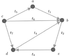
Figure 1: Graph representing a database

$E$	A	B
$t_{1}$	a	$b$
$t_{2}$	$b$	$e$
$t_{3}$	$e$	$d$
$t_{4}$	$d$	$b$
$t_{5}$	$c$	a
$t_{6}$	$c$	$b$
$t_{7}$	$c$	$d$

Consider the recursive Datalog query $\Pi$:

$${\it Ans}(x,y) \leftarrow P(x,y)$$

$$P(x,y) \leftarrow E(x,y)$$

$$P(x,y) \leftarrow P(x,z),E(z,y),$$

which collects pairs of vertices of $G$ that are connected through a path.

Since  $\Pi\cup D\models{\it Ans}(c,e)$, we have $\langle c,e\rangle$ as an answer to query $\Pi$ on $D$. This is because there are three distinct paths between $c$ and $e$ in $G$. All tuples except for $t_{3}$ are actual causes for this answer:  ${\it Causes}(E,\Pi(c,e))=\{t_{1},t_{2},t_{4},t_{5},t_{6},t_{7}\}$. We can see that all of these tuples contribute to at least one path between $c$ and $e$. Among them, $t_{2}$ has the highest responsibility, because, $t_{2}$ is a counterfactual cause for the answer, i.e. it has an empty contingency set. $\blacksquare$

The complexity of the computational and decision problems that arise in QA-causality have been investigated in [47, 59]. Here we recall those results that we will use throughout this work. The first problem is about deciding whether a tuple is an actual cause for a query answer.

Definition 1

For a Boolean monotone query $\mathcal{Q}$, the causality decision problem (CDP) is (deciding about membership of):

$\mathcal{CDP}(\mathcal{Q}):=\{(D,\tau)~{}|~{}\tau\in D^{n},\mbox{and }\tau\in{\it Causes}(D,\mathcal{Q})\}.$ $\blacksquare$

This problem is tractable for UCQs [47, 7], because it can be solved by CQ answering in relational databases. The next problem is about deciding if the responsibility of a tuple as a cause for a query answer is above a given threshold.

Definition 2

For a Boolean monotone query $\mathcal{Q}$, the responsibility decision problem (RDP) is (deciding about membership of):

$\mathcal{RDP}(\mathcal{Q})=\{(D,\tau,v)~{}|~{}\tau\in D^{n},v\in\{0\}\ \cup$
                                          $\{\frac{1}{k}~{}|~{}k\in\mathbb{N}^{+}\},$ $D\models\mathcal{Q}$  and  $\rho_{{}_{\!\mathcal{Q}\!}}^{D}(\tau)>v\}$. $\blacksquare$

This problem is NP-complete for CQs [47] and UCQs [59], but tractable for linear CQs [47]. Roughly speaking, a CQ is linear if its atoms can be ordered in a way that every variable appears in a continuous sequence of atoms that does not contain a self-join (i.e. a join involving the same predicate), e.g. $\exists xvyu(A(x)\wedge S_{1}(x,v)\wedge S_{2}(v,y)\wedge R(y,u)\wedge S_{3}(y,z))$ is linear, but not $\exists xyz(A(x)\wedge B(y)\wedge C(z)\wedge W(x,y,z))$, for which RDP is NP-complete [47].

The functional, non-decision, version of RDP is about computing responsibilities. This optimization problem is complete (in data) for ${\it FP}^{{\it{NP}(log}(n))}$ for UCQs [59]. Finally, we have the problem of deciding whether a tuple is a most responsible cause:

Definition 3

For a Boolean monotone query $\mathcal{Q}$, the most responsible cause decision problem is:

$\mathcal{MRCD}(\mathcal{Q})$ $=\{(D,\tau)~{}|~{}\tau\in D^{n}\ \mbox{and }0<\rho_{\mathcal{Q}}^{D}(\tau)\mbox{ is a maximum for }D\}$. $\blacksquare$

For UCQs this problem is complete for ${\it P}^{{\it{NP}(log}(n))}$ [59]. Hardness already holds for a CQ.

A notion of view-conditioned causality [48] will be formalized and investigated in Section 6.

4 Causality and Abduction

In general logical terms, an abductive explanation for an observation is a formula that, together with a background logical theory, entails the observation. Although one could see an abductive explanation as a cause for the observation, it has been argued that causes and abductive explanations are not necessarily the same [54, 24].

Under the abductive approach to diagnosis [19, 25, 52, 53], it is common that the system specification rather explicitly describes causal information, specially in action theories where the effects of actions are directly represented by positive definite rules. By restricting the explanation formulas to the predicates describing primitive causes (action executions), an explanation formula which entails an observation gives also a cause for the observation [24]. In this case, and is some sense, causality information is imposed by the system specifier  [52].

In database causality we do not have, at least not initially, a system description, but just a set of tuples. It is when we pose a query that we create something like a description, and the causal relationships between tuples are captured by the combination of atoms in the query. If the query is a Datalog query (in particular, a CQ), we have a specification in terms of positive definite rules.

In this section we will first establish connections between abductive diagnosis and database causality. We start by making precise the kind of abduction problems we will consider.

4.1 Background on Datalog abductive diagnosis

A Datalog abduction problem [26] is of the form $\mathcal{AP}=\langle\Pi,E,{\it Hyp},{\it Obs}\rangle$, where:  (a) $\Pi$ is a set of Datalog rules, (b) $E$ is a set of ground atoms (the extensional database), (c) ${\it Hyp}$, the hypothesis, is a finite set of ground atoms, the abducible atoms in this case, and (d) ${\it Obs}$, the observation, is a finite conjunction of ground atoms. As it is common, we will start with the assumption that $\Pi\cup E\cup{\it Hyp}\models{\it Obs}$. $\Pi\cup E$ is called the background theory (or specification).

Definition 4

Consider a Datalog abduction problem $\mathcal{AP}=\langle\Pi,E,{\it Hyp},{\it Obs}\rangle$.

1. An abductive diagnosis (or simply, a solution) for $\mathcal{AP}$ is a subset-minimal $\Delta\subseteq{\it Hyp}$, such that $\Pi\cup E\cup\Delta\models{\it Obs}$.

   This requires that no proper subset of $\Delta$ has this property. ${\it Sol}(\mathcal{AP})$ denotes the set of abductive diagnoses for problem $\mathcal{AP}$.

2. A hypothesis $h\in{\it Hyp}$ is relevant for $\mathcal{AP}$ if $h$ is contained in at least one diagnosis of $\mathcal{AP}$, otherwise it is irrelevant. ${\it Rel}(\mathcal{AP})$ collects all relevant hypothesis for $\mathcal{AP}$.

3. A hypothesis $h\in{\it Hyp}$ is necessary for $\mathcal{AP}$ if $h$ is contained in all diagnosis of $\mathcal{AP}$. ${\it Ness}(\mathcal{AP})$ collects all the necessary hypothesis for $\mathcal{AP}$. $\blacksquare$

Notice that for a problem $\mathcal{AP}$, ${\it Sol}(\mathcal{AP})$ is never empty due to the assumption $\Pi\cup D\cup{\it Hyp}\models{\it Obs}$. In case, $\Pi\cup D\models{\it Obs}$, it holds ${\it Sol}(\mathcal{AP})=\{\emptyset\}$.

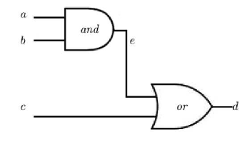
Figure 2: A simple circuite with two gates

Example 3. Consider the digital circuit in Figure 2. The inputs are $a=1$, $b=0$, $c=1$, but the output is $d=0$. So, the circuit is not working properly. The diagnosis problem is formulated below as a Datalog abduction problem whose data domain is $\{{\sf a},{\sf b},{\sf c},{\sf d},{\sf e},{\sf and},{\sf or}\}$. The underlying, extensional database is as follows: $E=\{{\it One}({\sf a}),{\it Zero}({\sf b}),$ ${\it One}({\sf c}),{\it And}({\sf a},{\sf b},{\sf e},{\sf and}),{\it Or}({\sf e},{\sf c},{\sf d},{\sf or}\}$.

The Datalog program $\Pi$ contains rules that model the normal and the faulty behavior of each gate. We show only the Datalog rules for the And gate. For its normal behavior, we have the following rules:

$${\it One}(O) \leftarrow {\it And}(I_{1},I_{2},O,G),{\it One}(I_{1}),{\it One}(I_{2})$$

$${\it Zero}(O) \leftarrow {\it And}(I_{1},I_{2},O,G),{\it One}(I_{1}),{\it Zero}(I_{2})$$

$${\it Zero}(O) \leftarrow {\it And}(I_{1},I_{2},O,G),{\it Zero}(I_{1}),{\it One}(I_{2})$$

$${\it Zero}(O) \leftarrow {\it And}(I_{1},I_{2},O,G),{\it Zero}(I_{1}),{\it One}(I_{2}).$$

The faulty behavior is modeled by the following rules:

$${\it Zero}(O) \leftarrow {\it And}(I_{1},I_{2},O,G),{\it One}(I_{1}),{\it One}(I_{2}),{\it Faulty}(G)$$

$${\it One}(O) \leftarrow {\it And}(I_{1},I_{2},O,G),{\it One}(I_{1}),{\it Zero}(I_{2}),{\it Faulty}(G)$$

$${\it One}(O) \leftarrow {\it And}(I_{1},I_{2},O,G),{\it Zero}(I_{1}),{\it One}(I_{2}),{\it Faulty}(G)$$

$${\it One}(O) \leftarrow {\it And}(I_{1},I_{2},O,G),{\it Zero}(I_{1}),{\it One}(I_{2}),{\it Faulty}(G)$$

Finally, we consider ${\it Obs}\!:{\it Zero}({\sf d})$, and ${\it Hyp}=\{{\it Faulty({\sf and})},{\it Faulty({\sf or})}\}$. The abduction problem consists in finding minimal $\Delta\subseteq{\it Hyp}$, such that $\Pi\cup E\cup\Delta\models{\it Zero}({\sf d})$. There is one abductive diagnosis: $\Delta=\{{\it Faulty({\sf or})}\}$. $\blacksquare$

In the context of Datalog abduction, we are interested in deciding, for a fixed Datalog program, if a hypothesis is relevant/necessary or not, with all the data as input. More precisely, we consider the following decision problems.

Definition 5

Given a Datalog program $\Pi$,

(a) The necessity decision problem (NDP) for $\Pi$ is  (deciding about the membership of):

$\mathcal{NDP}(\Pi)=\{({\it E,Hyp,Obs},h)~{}|~{}h\in{\it Ness}(\mathcal{AP}),\mbox{with }\mathcal{AP}=\langle\Pi,E,{\it Hyp},{\it Obs}\rangle\}$.

(b) The relevance decision problem (RLDP) for $\Pi$ is  (deciding about the membership of):

$\mathcal{RLDP}(\Pi)=\{({\it E,Hyp,Obs},h)~{}|~{}h\in{\it Rel}(\mathcal{AP}),\mbox{with }\mathcal{AP}=\langle\Pi,E,{\it Hyp},{\it Obs}\rangle\}$. $\blacksquare$

As it is common, we will assume that $|{\it Obs}|$, i.e. the number of atoms in the conjunction, is bounded above by a fixed parameter $p$. In many cases, $p=1$ (a single atomic observation).

The last two definitions suggest that we are interested in the data complexity of the relevance and necessity decision problems for Datalog abduction. That is, the Datalog program is fixed, but the data consisting of hypotheses and input structure $E$ may change. In contrast, under combined complexity the program is also part of the input, and the complexity is measured also in terms of the program size.

A comprehensive complexity analysis of several reasoning tasks on abduction from propositional logic programs, in particular of the relevance and necessity problems, can be found in [26]. Those results are all in combined complexity. In [26], it has been shown that for abduction from function-free first-order logic programs, the data complexity of each type of reasoning problem in the first-order case coincides with the complexity of the same type of reasoning problem in the propositional case. In this way, the next two results can be obtained for NDP and RLDP from [26, theo. 26] and the complexity of these problems for propositional Horn abduction (PDA), established in [27] (cf. also [25]). In the Appendix we provide direct, ad hoc proofs by adapting the full machinery developed in [26] for general programs. The next result follows from the membership of PTIME in data complexity of Datalog query evaluation (actually, this latter problem is PTIME-complete in data [22]).

Proposition 1

For every Datalog program, $\Pi$, $\mathcal{NDP}(\Pi)$ is in PTIME (in data). $\blacksquare$

Proposition 2

For Datalog programs $\Pi$, $\mathcal{RLDP}(\Pi)$ is NP-complete  (in data). $\blacksquare$

It is clear from this result that deciding relevance for Datalog abduction is also intractable in combined complexity. However, a tractable case of combined complexity is identified in [32], on the basis of the notions of tree-decomposition and bounded tree-width, which we now briefly present.

Let $\mathcal{H}=\langle V,H\rangle$ be a hypergraph, where $V$ is the set of vertices, and $H$ is the set of hyperedges, i.e. of subsets of $V$. A tree-decomposition of $\mathcal{H}$ is a pair $(\mathcal{T},\lambda)$, where $\mathcal{T}=\langle N,E\rangle$ is a tree and $\lambda$ is a labeling function that assigns to each node $n\in N$, a subset $\lambda(n)$ of $V$ ($\lambda(n)$ is aka. bag), i.e. $\lambda(n)\subseteq V$, such that, for every node $n\in N$, the following hold:  (a) For every $v\in V$, there exists $n\in N$ with $v\in\lambda(n)$.  (b) For every $h\in H$, there exists a node $n\in N$ with $h\subseteq\lambda(n)$.  (c) For every $v\in V$, the set of nodes $\{n~{}|~{}v\in\lambda(n)\}$ induces a connected subtree of $\mathcal{T}$.

The width of a tree decomposition $(\mathcal{T},\lambda)$ of $\mathcal{H}=\langle V,H\rangle$, with $\mathcal{T}=\langle N,E\rangle$, is defined as ${\it max}\{|\lambda(n)|-1\ :\ n\in N\}$. The tree-width $t_{w}(\mathcal{H})$ of $\mathcal{H}$ is the minimum width over all its tree decompositions.

Intuitively, the tree-width of a hypergraph $\mathcal{H}$ is a measure of the “tree-likeness” of $\mathcal{H}$. A set of vertices that form a cycle in $\mathcal{H}$ are put into a same bag, which becomes (the bag of a) node in the corresponding tree-decomposition. If the tree-width of the hypergraph under consideration is bounded by a fixed constant, then many otherwise intractable problems become tractable [31].

It is possible to associate an hypergraph to any finite structure $D$ (think of a relational database): If its universe (the active domain in the case of a relational database) is $V$, define the hypergraph $\mathcal{H}(D)=(V,H)$, with $H=\{~{}\{a_{1},\ldots,a_{n}\}~{}|~{}D$ contains a ground atom $P(a_{1}\ldots a_{n})$ for some predicate symbol $P\}$.

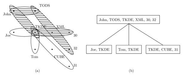
Figure 3:  (a)  $\mathcal{H}(D)$.    (b)  A tree decomposition of $\mathcal{H}(D)$.

Example 4. Consider instance $D$ in Example 3.1. The hypergraph $\mathcal{H}(D)$ associated to $D$ is shown in Figure 3(a). Its vertices are the elements of ${\it Adom}(D)=\{{\sf John},{\sf Joe},{\sf Tom},{\sf TODS},{\sf TKDE},{\sf XML},{\sf CUBE},\mbox{ 30, 31, 32}\}$, the active domain of $D$. For example, since ${\it Journal}({\sf TKDE},{\sf XML},\mbox{30})\in D$, $\{{\sf TKDE},{\sf XML},\mbox{30}\}$ is one of the hyperedges.

The dashed ovals show four sets of vertices, i.e. hyperedges, that together form a cycle. Their elements are put into the same bag of the tree-decomposition. Figure 3(b) shows a possible tree-decomposition of $\mathcal{H}(D)$. In it, the maximum $|\lambda(n)|-1$ is $6-1$, corresponding to the top box bag of the tree. So, $t_{w}(\mathcal{H}(D))\leq 5$. $\blacksquare$

The following is a fixed-parameter tractability result for the relevance decision problem for Datalog abduction for guarded programs $\Pi$, where in every rule body there is an atom that contains (guards) all the variables appearing in that body.

Theorem 1

[32, theo. 7.9]  Let $k$ be an integer. For Datalog abduction problems $\mathcal{AP}=\langle\Pi,E,{\it Hyp},{\it Obs}\rangle$ where $\Pi$ is guarded, and $t_{w}(\mathcal{H}(E))\leq k$, relevance can be decided in polynomial time in $|\mathcal{AP}|$. More precisely, the following decision problem is tractable:

$\mathcal{RLDP}=\{(\langle\Pi,{\it E,Hyp,Obs}\rangle,h)~{}|~{}h\in{\it Rel}(\langle\Pi,{\it E,Hyp,Obs}\rangle),h\in{\it Hyp},$
                                                      $\Pi\mbox{ is guarded, and }t_{w}(\mathcal{H}(E))\leq k\}$. $\blacksquare$

This is a case of tractable combined complexity with a fixed parameter that is the tree-width of the extensional database.

In the rest of this section we assume, unless otherwise stated, that we have a partitioned relational instance $D=D^{x}\cup D^{n}$.

4.2 Actual causes from abductive diagnoses

In this section we show that, for Datalog system specifications, abductive inference corresponds to actual causation. That is, abductive diagnoses for an observation essentially contain actual causes for the observation.

Consider that $\Pi$ is a Boolean, possibly recursive Datalog query; and assume that $\Pi\cup D\models{\it ans}$. Then, the decision problem in Definition 1 takes the form:

$$\mathcal{CDP}(\Pi):=\{(D,\tau)~{}|~{}\tau\in D^{n},\mbox{and }\tau\in{\it Causes}(D,\Pi)\}.$$ (2)

We now show that actual causes for ${\it ans}$ can be obtained from abductive diagnoses of the associated causal Datalog abduction problem (CDAP):   $\mathcal{AP}^{c}:=\langle\Pi,D^{x},D^{n},{\it ans}\rangle$, where $D^{x}$ takes the role of the extensional database for $\Pi$. Accordingly, $\Pi\cup D^{x}$ becomes the background theory, $D^{n}$ becomes the set of hypothesis, and atom ${\it ans}$ is the observation.

Proposition 3

For an instance $D=D^{x}\cup D^{n}$ and a Boolean Datalog query $\Pi$, with $\Pi\cup D\models{\it ans}$, and its associated CDAP $\mathcal{AP}^{c}$, the following hold:

1. $\tau\in D^{n}$ is an counterfactual cause for ${\it ans}$ iff $\tau\in{\it Ness}(\mathcal{AP}^{c})$.

2. $\tau\in D^{n}$ is an actual cause for ${\it ans}$ iff $\tau\in{\it Rel}(\mathcal{AP}^{c})$.

Proof: Part (a) is straightforward. To proof part (b), first assume $\tau$ is an actual cause for ans. According to the definition of an actual cause, there exists a contingency set $\Gamma\subseteq D^{n}$ such that $\Pi\cup D\smallsetminus\Gamma\models{\it ans}$ but $\Pi\cup D\smallsetminus(\Gamma\cup\{\tau\})\not\models{\it ans}$. This implies that there exists a set $\Delta\subseteq D^{n}$ with $\tau\in\Delta$ such that $\Pi\cup\Delta\models{\it ans}$. It is easy to see that $\Delta$ is an abductive diagnosis for $\mathcal{AP}^{c}$. Therefore, $\tau\in{\it Rel}(\mathcal{AP}^{c})$.

Second, assume $\tau\in{\it Rel}(\mathcal{AP}^{c})$. Then there exists a set $\mathcal{S}_{k}\in{\it Sol}(\mathcal{AP}^{c})=\{s_{1}\ldots s_{n}\}$ such that $\mathcal{S}_{k}\models{\it ans}$ with $\tau\in\mathcal{S}_{k}$. Obviously, ${\it Sol}(\mathcal{AP}^{c})$ is a collection of subsets of $D^{n}$. Pick a set $\Gamma\subseteq D^{n}$ such that for all $\mathcal{S}_{i}\in{\it Sol}(\mathcal{AP}^{c})$ $i\not=k$, $\Gamma\cap\mathcal{S}_{i}\not=\emptyset$ and $\Gamma\cap\mathcal{S}_{k}=\emptyset$. It is clear that $\Pi\cup D\smallsetminus(\Gamma\cup\{t\})\not\models{\it ans}$ but $\Pi\cup D\smallsetminus\Gamma\models{\it ans}$. Therefore, $\tau$ is an actual cause for ans. To complete the proof we need to show that such $\Gamma$ always exists. This can be done by applying the digitalization technique to construct such $\Gamma$. Since all elements of ${\it Sol}(\mathcal{AP}^{c})$ are subset-minimal, then, for each $\mathcal{S}_{i}\in{\it Sol}(\mathcal{AP}^{c})$ with $i\not=k$, there exists a $\tau^{\prime}\in\mathcal{S}_{i}$ such that $\tau^{\prime}\not\in\mathcal{S}_{k}$. So, $\Gamma$ can be obtained from the union of differences between each $\mathcal{S}_{i}$ ($i\not=k$) and $\mathcal{S}_{k}$. $\blacksquare$

Example 5. Consider the instance $D$ with relations $R$ and $S$ as below, and the

query $\Pi\!:\ {\it ans}\leftarrow R(x,y),S(y)$, which is true in $D$. Assume all tuples are endogenous.

$R$	A	B
	$a_{1}$	$a_{4}$
	$a_{2}$	$a_{1}$
	$a_{3}$	$a_{3}$

$S$	B
	$a_{1}$
	$a_{2}$
	$a_{3}$

In this case, $\mathcal{AP}^{c}=\langle\Pi,\emptyset,D,{\it ans}\rangle$, which has two (subset-minimal) abductive diagnoses: $\Delta_{1}=\{S(a_{1}),R(a_{2},a_{1})\}$ and $\Delta_{2}=\{S(a_{3}),R(a_{3},a_{3})\}$. Then, ${\it Rel}(\mathcal{AP}^{c})=\{S(a_{3}),$ $R(a_{3},a_{3}),$ $S(a_{1}),R(a_{2},a_{1})\}$. It is easy to see that the relevant hypothesis are actual causes for ${\it ans}$. $\blacksquare$

4.3 Causal responsibility and abductive diagnosis

In the previous section we showed that counterfactual and actual causes for Datalog query answers appear as necessary and relevant hypotheses in the associated Datalog abduction problem. The form causal responsibility takes in Datalog abduction is less direct. Actually, we first show that causal responsibility inspires an interesting concept for Datalog abduction, that of degree of necessity of a hypothesis.

Example 6. (ex. 3 cont.) Consider now $D^{\prime}=\{R(a_{1},a_{3}),R(a_{2},a_{3}),S(a_{3})\}$, and $\mathcal{AP}^{c}=\langle\Pi,\emptyset,D^{\prime},{\it ans}\rangle$.  $\mathcal{AP}^{c}$ has two abductive diagnosis: $\Delta_{1}=\{S(a_{3}),R(a_{1},a_{3})\}$ and $\Delta_{2}=\{S(a_{3}),R(a_{2},a_{3})\}$.

Here, ${\it Ness}(\mathcal{AP}^{c})=\{S(a_{3})\}$, i.e. only $S(a_{3})$ is necessary for abductively explaining ${\it ans}$. However, this is not capturing the fact that $R(a_{1},a_{3})$ or $R(a_{3},a_{3})$ are also needed as a part of the explanation. $\blacksquare$

This example suggests that necessary hypotheses might be better captured as sets of them rather than as individuals.

Definition 6

Given a DAP, $\mathcal{AP}=\langle\Pi,E,{\it Hyp},{\it Obs}\rangle$,  $N\subseteq{\it Hyp}$ is a necessary-hypothesis set if: (a) for $\mathcal{AP}_{\!\!-N}:=\langle\Pi,E,{\it Hyp}\smallsetminus N,{\it Obs}\rangle$, ${\it Sol}(\mathcal{AP}_{\!\!-N})=\emptyset$, and (b) $N$ is subset-minimal, i.e. no proper subset of $N$ has the previous property. $\blacksquare$

It is easy to verify that a hypothesis $h$ is necessary according to Definition 4 iff $\{h\}$ is a necessary-hypothesis set.

If we apply Definition 6 to $\mathcal{AP}^{c}$ in Example 4.3, we obtain two necessary-hypothesis sets: $N_{1}=\{S(a_{3})\}$ and $N_{2}=\{R(a_{1},a_{3}),R(a_{2},a_{3})\}$. In this case, it makes sense to claim that $S(a_{3})$ is more necessary for explaining ${\it ans}$ than the other two tuples, that need to be combined. Actually, we can think of ranking hypothesis according to the minimum cardinality of necessary-hypothesis sets where they are included.

Definition 7

Given a DAP, $\mathcal{AP}=\langle\Pi,E,{\it Hyp},{\it Obs}\rangle$, the necessity-degree of a hypothesis $h\in Hyp$ is $\eta_{{}_{\!\mathcal{AP}{}\!}}(h):=\frac{1}{|N|}$ where, $N$ is a minimum-cardinality necessary-hypothesis set with $h\in N$. If $h$ does not belong to any necessary hypothesis set, $\eta_{{}_{\!\mathcal{AP}{}\!}}(h):=0$. $\blacksquare$

Example 7. (ex. 4.3 cont.)  We have  $\eta_{{}_{\!\mathcal{AP}^{c}{}\!}}(S(a_{3}))=1$ and $\eta_{{}_{\!\mathcal{AP}^{c}{}\!}}(R(a_{2},a_{3}))=\eta_{{}_{\!\mathcal{AP}^{c}{}\!}}(R(a_{1},a_{3}))=\frac{1}{2}$. Now, if we consider the original Datalog query in the causality setting, where $\Pi\cup D^{\prime}\models{\it ans}$, then $S(a_{3}),R(a_{2},a_{3}),R(a_{1},a_{3})$ are all actual causes, with responsibilities: $\rho_{{}_{\!\Pi\!}}^{D}(S(a_{3}))=1$, $\rho_{{}_{\!\Pi\!}}^{D}(R(a_{2},a_{3}))$ $=\rho_{{}_{\!\Pi\!}}^{D}(R(a_{1},a_{3}))$ $=\frac{1}{2}$. This is not a coincidence. In fact the notion of causal responsibility is in correspondence with the notion of necessity degree in the Datalog abduction setting. $\blacksquare$

Proposition 4

Let $D=D^{x}\cup D^{n}$ be an instance and $\Pi$ be a Boolean Datalog query with $\Pi\cup D\models{\it ans}$, and $\mathcal{AP}^{c}$ its associated CDAP. For $\tau\in D^{n}$, it holds: $\eta_{{}_{\!\mathcal{AP}^{c}\!}}(\tau)=\rho_{{}_{\!\Pi\!}}^{D}(\tau)$.

Proof: It is easy to verify that each actual cause, together with a contingency set, forms a necessary hypothesis set for the corresponding causal Datalog abduction setting (and the other way around). Then, the two values are in correspondence. $\blacksquare$

Notice that the notion of necessity-degree is interesting and applicable to general abduction from logical theories, that may not necessarily represent causal knowledge about a domain. In this case, the necessity-degree is not a causality-related notion, and merely reflects the extent by which a hypothesis is necessary for making an observation explainable within an abductive theory.

4.4 Abductive diagnosis from actual causes

Now we show, conversely, that QA-causality can capture Datalog abduction. In particular, we show that abductive diagnoses from Datalog programs are formed essentially by actual causes for the observation. More precisely, consider a Datalog abduction problem $\mathcal{AP}=\langle\Pi,E,{\it Hyp},{\it Obs}\rangle$, where $E$ is the underlying extensional database, and ${\it Obs}$ is a conjunction of ground atoms. For this we need to construct a QA-causality setting.

Proposition 5

Let $\mathcal{AP}=\langle\Pi,E,{\it Hyp},{\it Obs}\rangle$ be a Datalog abduction problem, and $h\in{\it Hyp}$. It holds that $h$ is a relevant hypothesis for $\mathcal{AP}$, i.e. $h\in{\it Rel}(\mathcal{AP})$, iff $h$ is an actual cause for the associated Boolean Datalog query $\Pi^{c}:=\Pi\ \cup\ \{{\it ans}\leftarrow{\it Obs}\}$ being true in $D:=D^{x}\cup D^{n}$ with $D^{x}:=E$, and $D^{n}:={\it Hyp}$. Here, ans is a fresh propositional atom. $\blacksquare$

The proof is similar to that of Proposition 3, where we start with a causality setting, producing an abductive setting. Instead, in this case we start from an abductive setting and produce a causal one.

Example 8. (ex. 2 cont.)  For the given DAP $\mathcal{AP}$, we construct a QA-causality setting as follows. Consider the instance $D$ with relations And, Or, ${\it Faulty}$, One and Zero, as below, and the Boolean Datalog query $\Pi^{c}\!:\ \Pi\ \cup\ \{{\it ans}\leftarrow{\it Zero}({\sf d})\}$, where $\Pi$ is the Datalog program in Example 2.

And	$I_{1}$	$I_{2}$	$O$	$G$
	a	b	e	and

${\it Zero}$	I
	b

Or	$I_{1}$	$I_{2}$	$O$	$G$
	e	c	d	or

${\it One}$	I
	a
	c

${\it Faulty}$	$G$
	and
	or

It clear that $\Pi^{c}\cup D\models{\it ans}$. $D$ is partitioned into the set of endogenous tuples $D^{n}:=\{{\it Faulty({\sf and})},$ ${\it Faulty({\sf or})}\}$ and the set of exogenous tuples $D^{x}:=D\smallsetminus D^{n}$.

It is easy to verify that this result has only one actual cause, namely ${\it Faulty({\sf or})}$ (with responsibility 1), confirming the correspondence with Example 2 as stated in Proposition 5. $\blacksquare$

4.5 Complexity of causality for Datalog queries

Now we use the results obtained so far in this section to obtain new complexity results for Datalog QA-causality. We first consider the problem of deciding if a tuple is a counterfactual cause for a query answer.

A counterfactual cause is a tuple that, when removed from the database, undermines the query-answer, without having to remove other tuples, as is the case for actual causes. Actually, for each of the latter there may be an exponential number of contingency sets, i.e. of accompanying tuples [59]. Notice that a counterfactual cause is an actual cause with responsibility $1$.

Definition 8

For a Boolean monotone query $\mathcal{Q}$, the counterfactual causality decision problem (CFDP) is (deciding about membership of):

$\mathcal{CFDP}(\mathcal{Q}):=\{(D,\tau)~{}|~{}\tau\in D^{n}\mbox{ and }\rho_{{}_{\!\mathcal{Q}\!}}^{D}(\tau)=1\}.$ $\blacksquare$

The complexity of this problem can be obtained from the connection between counterfactual causation and the necessity of hypothesis in Datalog abduction via Propositions 1 and 3.

Proposition 6

For Boolean Datalog queries $\Pi$, $\mathcal{CFDP}(\Pi)$ is in PTIME  (in data).

Proof: Directly from Propositions 1 and 3. $\blacksquare$

Now we address the complexity of the actual causality problem for Datalog queries. The following result is obtained from Propositions 2 and 5.

Proposition 7

For Boolean Datalog queries $\Pi$, $\mathcal{CDP}(\Pi)$ is NP-complete (in data).

Proof: To show the membership of NP, consider an instance $D=D^{n}\cup D^{x}$ and a tuple $\tau\in D^{n}$. To check if $(D,\tau)\in\mathcal{CDP}(\Pi)$ (equivalently $\tau\in{\it Causes}(D,\Pi))$, non-deterministically guess a subset $\Gamma\subseteq D^{n}$, return yes if $\tau$ is a counterfactual cause for $\mathcal{Q}(\bar{a})$ in $D\smallsetminus\Gamma$, and no otherwise. By Proposition 6 this can be done in polynomial time.

The NP-hardness is obtained by a reduction from the relevance problem for Datalog abduction to causality problem, as given in Proposition 5. $\blacksquare$

This result should be contrasted with the tractability of the same problem for UCQs [59]. In the case of Datalog, the NP-hardness requires a recursive query. This can be seen from the proof of Proposition 7, which appeals in the end to the NP-hardness in Proposition 2, whose proof uses a recursive query (program) (cf. the query given by (13)-(14) in the Appendix).

We now introduce a fixed-parameter tractable case of the actual causality problem. Actually, we consider the “combined” version of the decision problem in Definition 1, where both the Datalog query and the instance are part of the input. For this, we take advantage of the tractable case of Datalog abduction presented in Section 4.1. The following is an immediate consequence of Theorem 1 and Proposition 3.

Proposition 8

For a guarded Boolean Datalog query $\Pi$, an instance $D=D^{x}\cup D^{n}$, with $D^{x}$ of bounded tree-width, and $\tau\in D^{n}$, deciding if $\tau\in{\it Causes}(D,\Pi)$ is fixed-parameter tractable (in combined complexity), and the parameter is the tree-width bound. $\blacksquare$

Finally, we establish the complexity of the responsibility problem for Datalog queries.

Proposition 9

For Boolean Datalog queries $\Pi$, $\mathcal{RDP}(\Pi)$ is NP-complete. $\blacksquare$

Proof:  To show membership of NP, consider an instance $D=D^{n}\cup D^{x}$, a tuple $\tau\in D^{n}$, and a responsibility bound $v$. To check if $\rho_{{}_{\!\Pi\!}}^{D}(\tau)>v$, non-deterministically guess a set $\Gamma\subseteq D^{n}$ and check if $\Gamma$ is a contingency set and $\Gamma<\frac{1}{v}$. The verification can be done in polynomial time. Hardness is obtain from the NP-completeness of RDP for conjunctive queries established in [59]. $\blacksquare$

5 Causality and View-Updates

There is a close relationship between QA-causality and the view-update problem in the form of delete-propagation. It was first suggested in [42, 43], and here we investigate it more deeply. We start by formalizing some computational problems related to the general delete-propagation problem that are interesting from the perspective of QA-causality.

5.1 Background on delete-propagation

Given a monotone query $\mathcal{Q}$, we can think of it as defining a view, $\mathcal{V}$, with virtual contents $\mathcal{Q}(D)$. If $\bar{a}\in\mathcal{Q}(D)$, which may not be intended, we may try to delete some tuples from $D$, so that $\bar{a}$ disappears from $\mathcal{Q}(D)$. This is a particular case of database updates through views [1], and may appear in different and natural formulations. The next example shows one of them.

Example 9.   Consider relational predicates  ${\it GroupUser(User,Group})$  and ${\it GroupFile(File,Group})$, with extensions as in instance $D$ below. They represent users’ memberships of groups, and access permissions for groups to files, respectively.

GroupUser	User	Group
	Joe	$g_{1}$
	Joe	$g_{2}$
	John	$g_{1}$
	Tom	$g_{2}$
	Tom	$g_{3}$
	John	$g_{3}$

GroupFiles	File	Group
	$f_{1}$	$g_{1}$
	$f_{1}$	$g_{3}$
	$f_{2}$	$g_{2}$
	$f_{3}$	$g_{3}$

It is expected that a user $u$ can access file $f$ if $u$ belongs to a group that can access $f$, i.e. there is some group $g$ such that ${\it GroupUser}(u,g)$ and ${\it GroupFile}(f,g)$ hold. Accordingly, we can define a view that collects users with the files they can access, as defined by the following query:

$${\it Access(User,File})\ \leftarrow\ {\it GroupUser(User,Group),GroupFile(File,Group}).$$ (3)

Query ${\it Access}$ in (3) has the following answers, providing a view extension:

${\it Access}(D)$	User	File
	Joe	$f_{1}$
	Joe	$f_{2}$
	Tom	$f_{1}$
	Tom	$f_{2}$
	Tom	$f_{3}$
	John	$f_{1}$
	John	$f_{3}$

ooo

In a particular version of the delete-propagation problem, the objective may be to delete a minimum number of tuples from the instance, so that an authorized access (unexpected answer to the query) is deleted from the query answers, while all other authorized accesses (other answers to the query) remain intact. $\blacksquare$

In the following, we consider several variations of this problem, both in their functional and decision versions.

Definition 9

Let $D$ be a database instance, and $\mathcal{Q}(\bar{x})$ a monotone query.

1. For $\bar{a}\in\mathcal{Q}(D)$, the minimal-source-side-effect deletion-problem is about computing a subset-minimal $\Lambda\subseteq D$, such that $\bar{a}\ \notin\mathcal{Q}(D\smallsetminus\Lambda)$.

2. The minimal-source-side-effect decision problem is (deciding about the membership  of):

   $\mathcal{MSSEP}^{s\!}(\mathcal{Q})=\{(D,D^{\prime},\bar{a})~{}|~{}\bar{a}\in\mathcal{Q}(D),\ D^{\prime}\subseteq D,\bar{a}\not\in\mathcal{Q}(D^{\prime}),\mbox{ and}$
                                                                        $D^{\prime}\mbox{ is subset-maximal}\}$.
   (The superscript $s$ stands for subset-minimal.)

3. For $\bar{a}\in\mathcal{Q}(D)$, the minimum-source-side-effect deletion-problem is about computing a minimum-cardinality $\Lambda\subseteq D$, such that $\bar{a}\notin\mathcal{Q}(D\smallsetminus\Lambda)$.

4. The minimum-source-side-effect decision problem is (deciding about the membership of):

   $\mathcal{MSSEP}^{c\!}(\mathcal{Q})=\{(D,D^{\prime},\bar{a})~{}|~{}\bar{a}\in\mathcal{Q}(D),D^{\prime}\subseteq D,\ \bar{a}\notin\mathcal{Q}(D^{\prime}),\mbox{ and }$
                                                            $D^{\prime}\mbox{ has maximum cardinality}\}$.
   (Here, $c$ stands for cardinality.) $\blacksquare$

Definition 10

[12]  Let $D$ be a database instance $D$, and $\mathcal{Q}(\bar{x})$ a monotone query.

1. For $\bar{a}\in\mathcal{Q}(D)$, the view-side-effect-free deletion-problem is about computing a $\Lambda\subseteq D$, such that $\mathcal{Q}(D)\smallsetminus\{\bar{a}\}=\mathcal{Q}(D\smallsetminus\Lambda)$.

2. The view-side-effect-free decision problem is (deciding about the membership of):

   $\mathcal{VSEFP}(\mathcal{Q})=\{(D,\bar{a})~{}|~{}\bar{a}\in\mathcal{Q}(D),\ \mbox{and exists }D^{\prime}\subseteq D\mbox{ with }$
                                                                   $\mathcal{Q}(D)\smallsetminus\{\bar{a}\}=\mathcal{Q}(D^{\prime})\}$. $\blacksquare$

The decision problem in Definition 10(b) is NP-complete for conjunctive queries [12, theorem 2.1]. Notice that, in contrast to those in (a) and (c) in Definition 9, this decision problem does not involve a candidate $D^{\prime}$, and only asks about its existence. This is because candidates always exist for Definition 9, whereas for the view-side-effect-free deletion-problem there may be no sub-instance that produces exactly the intended deletion from the view. As usual, there are functional problems associated to $\mathcal{VSEFP}$, about computing a maximal/maximum $D^{\prime}$ that produces the intended side-effect free deletion; and also the two corresponding decision problems about deciding concrete candidates $D^{\prime}$.

Example 10. (ex. 3.1 cont.)  Consider the instance $D$ and the conjunctive query $\mathcal{Q}$ in (3.1). Assume that XML is not among John’s research interests, so that tuple $\langle{\sf John},{\sf XML}\rangle$ in the view $\mathcal{Q}(D)$ is unintended. We want to find tuples in $D$ whose removal leads to the deletion of this view tuple. There are multiple ways to achieve this goal.

Notice that the tuples in $D$ related to answer $\langle{\sf John},{\sf XML}\rangle$ through the query are Author(John, TKDE), Journal(TODS, XML, 32), Author(John, TODS) and Journal(TKDE, XML,30). They are all candidates for removal. However, the decision problems described above impose different conditions on what are admissible deletions.

(a) Source-side effect: The objective is to find minimal/minimum sets of tuples whose removal leads to the deletion of $\langle{\it\sf John},{\sf{\sf XML}}\rangle$. One solution is removing $S_{1}$={Author(John, TODS), Author(John, TKDE)} from the Author table. The other solution is removing $S_{2}$={Journal(TODS, XML,30), Journal(TKDE, XML, 30)} from the Journal table.

Furthermore, the removal of either $S_{3}=\{{\it Author}({\sf John},{\sf TKDE}),$ ${\it Journal}({\sf TODS},$ ${\sf XML},\mbox{32})\}$ or $S_{4}=\{{\it Author}({\sf John},{\sf TODS}),{\it Journal}({\sf TKDE},{\sf XML},$ $\mbox{30})\}$ eliminates the intended view tuple. Thus, $S_{1}$, $S_{2}$, $S_{3}$ and $S_{4}$ are solutions to both the minimum- and minimal-source side-effect deletion-problems.

(b) View-side effect: Removing any of the sets $S_{1}$, $S_{2}$, $S_{3}$ or $S_{4}$, leads to the deletion of $\langle{\sf John},{\sf XML}\rangle$. However, we now want those sets whose elimination produce no side-effects on the view. That is, their deletion triggers the deletion of $\langle{\sf John},{\sf XML}\rangle$ from the view, but not of any other tuple in it.

None of the sets $S_{1}$, $S_{2}$, $S_{3}$ and $S_{4}$ is side-effect free. For example, the deletion of $S_{1}$ also results in the deletion of $\langle{\sf John},{\sf CUBE}\rangle$ from the view. $\blacksquare$

Example 11. (ex. 5.1 cont.)  It is easy to verify that there is no solution to the view-side-effect-free deletion-problem for answer $\langle{\sf Tom},f_{3}\rangle$ (in the view extension ${\it Access}$). To eliminate this entry from the view, either ${\it GroupUser}({\sf Tom},g_{3})$ or ${\it GroupFiles}(f_{3},g_{3})$ must be deleted from $D$. Removing the former results in the additional deletion of $\langle{\sf Tom},f_{1}\rangle$ from the view; and eliminating the latter, results in the additional deletion of $\langle{\sf John},f_{3}\rangle$.

However, for the answer $\langle{\sf Joe},f_{1}\rangle$, there is a solution to the view-side-effect-free deletion-problem, by removing ${\it GroupUser}({\sf Joe},g_{1})$ from $D$. This deletion does not have unintended side-effects on the view contents. $\blacksquare$

5.2 QA-causality and delete-propagation

In this section we first establish mutual reductions between the delete-propagation problems and QA-causality.

5.2.1 Delete propagation from QA-causality.  

In this section, unless otherwise stated, all the database tuples are assumed to be endogenous.

Consider a relational instance $D$, a view $\mathcal{V}$ defined by a monotone query $\mathcal{Q}$. Then, the virtual view extension, $\mathcal{V}(D)$, is $\mathcal{Q}(D)$.

For a tuple $\bar{a}\in{\color[rgb]{0,0,1}\mathcal{Q}}(D)$, the delete-propagation problem, in its most general form, is about deleting a set of tuples from $D$, and so obtaining a subinstance $D^{\prime}$ of $D$, such that $\bar{a}\notin\mathcal{Q}(D^{\prime})$. It is natural to expect that the deletion of $\bar{a}$ from ${\color[rgb]{0,0,1}\mathcal{Q}}(D)$ can be achieved through deletions from $D$ of actual causes for $\bar{a}$ (to be in the view extension). However, to obtain solutions to the different variants of this problem introduced in Section 5.1, different combinations of actual causes must be considered.

First, we show that an actual cause for $\bar{a}$ forms, with any of its contingency sets, a solution to the minimal-source-side-effect deletion-problem associated to $\bar{a}$ (cf. Definition 9).

Proposition 10

For an instance $D$, a subinstance $D^{\prime}\subseteq D$, a view defined by a monotone query $\mathcal{Q}(\bar{x})$, and $\bar{a}\in\mathcal{Q}(D)$,   $(D,D^{\prime},\bar{a})\in\mathcal{MSSEP}^{s\!}(\mathcal{Q})$  iff  there is a $\tau\in D\smallsetminus D^{\prime}$, such that $\tau\in{\it Causes}(D,\mathcal{Q}(\bar{a}))$ and $D\smallsetminus(D^{\prime}\cup\{\tau\})\in{\it Cont}^{s}(D,\mathcal{Q}(\bar{a}),\tau)$.

Proof: Suppose first that $(D,D^{\prime},\bar{a})\in\mathcal{MSSEP}^{s\!}(\mathcal{Q})$. Then, according to Definition 9, $\bar{a}\not\in\mathcal{Q}(D^{\prime})$. Let $\Lambda=D\smallsetminus D^{\prime}$. For an arbitrary element $\tau\in\Lambda$ (clearly, $\Lambda\not=\emptyset$), let $\Gamma:=\Lambda\smallsetminus\{\tau\}$. Due to the subset-maximality of $D^{\prime}$ (then, subset-minimality of $\Lambda$), we obtain: $D\smallsetminus(\Gamma\cup\{\tau\})\not\models\mathcal{Q}(\bar{a})$, but $D\smallsetminus\Gamma\models\mathcal{Q}(\bar{a})$. Therefore, $\tau$ is an actual cause for $\bar{a}$.

For the other direction, suppose $\tau\in{\it Causes}(D,\mathcal{Q}(\bar{a}))$ and $D\smallsetminus(D^{\prime}\cup\{\tau\})\in{\it Cont}^{s}(D,\mathcal{Q}(\bar{a}),\tau)$. Let $\Gamma:=D\smallsetminus(D^{\prime}\cup\{\tau\})$. From the definition of an actual cause, we obtain that $\bar{a}\ \notin\mathcal{Q}(D\smallsetminus(\Gamma\cup\{\tau\})$. So, $\bar{a}\ \notin\mathcal{Q}(D^{\prime})$ (notice that $D^{\prime}=D\smallsetminus(\Gamma\cup\{\tau\}$). Since $\Gamma$ is a subset-minimal contingency set for $\tau$, $D^{\prime}$ is a subset-maximal subinstance that enjoys the mentioned property. So, $(D,D^{\prime},\bar{a})\in\mathcal{MSSEP}^{s\!}(\mathcal{Q})$. $\blacksquare$

Corollary 1

For a view defined by a monotone query, deciding if a set of source deletions producing the deletion from the view is subset minimal is in polynomial time in data.

Proof: This follows from the connection between QA-causality and delete-propagation established in Proposition 10, and the fact that deciding a cause for a monotone query and deciding the subset minimality of an associated contingency set candidate are both in polynomial time in data [47, 7]. $\blacksquare$

We show next that, in order to minimize the number of side-effects on the source (the problem in Definition 9(c)), it is good enough to pick a most responsible cause for $\bar{a}$ with any of its minimum-cardinality contingency sets.

Proposition 11

For an instance $D$, a subinstance $D^{\prime}\subseteq D$, a view $\mathcal{V}$ defined by a monotone query $\mathcal{Q}$, and $\bar{a}\in\mathcal{Q}(D)$,   $(D,D^{\prime},\bar{a})\in\mathcal{MSSEP}^{c\!}(\mathcal{Q})$  iff  there is a $\tau\in D\smallsetminus D^{\prime}$, such that $\tau\in\mathcal{MRC}(D,\mathcal{Q}(\bar{a}))$, $\Gamma:=D\smallsetminus(D^{\prime}\cup\{\tau\})\in{\it Cont}^{s}(D,\mathcal{Q}(\bar{a}),\tau)$, and there is no $\Gamma^{\prime}\in{\it Cont}^{s}(D,\mathcal{Q}(\bar{a}),\tau)$ with $|\Gamma^{\prime}|<|\Gamma|$.

Proof: Similar to the proof of Proposition 10. $\blacksquare$

In relation to the problems involved in this proposition, the decision problems associated to computing a minimum-side-effect source deletion and computing the responsibility of a cause, both for monotone queries, have been independently established as NP-complete in data, in [12] and [7], resp.

Example 12. (ex. 10 cont.) We obtained the followings solutions to the minimum- (and also minimal-) source-side-effect deletion-problem for the view tuple $\langle{\it{\sf John},{\sf XML}}\rangle$:

$$S_{1} = \{{\it Author({\sf John},{\sf TODS}),Author({\sf John},{\sf TKDE})}\},$$

$$S_{2} = \{{\it Journal}({\sf TODS},{\sf XML},\mbox{30}),Journal({\sf TKDE},{\sf XML},\mbox{30})\},$$

$$S_{3} = \{{\it Author}({\sf John},{\sf TKDE}),Journal({\sf TODS},{\sf XML},\mbox{32})\},$$

$$S_{4} = \{{\it Author}({\sf John},{\sf TODS}),Journal({\sf TKDE},{\sf XML},\mbox{30})\}.$$

On the other side, in Example 3.1, we showed that the tuples Author(John,TODS), Journal(TKDE,XML,30), Author(John,TKDE), and Journal(TODS, XML,32) are actual causes for the answer $\langle{\it\sf John},{\sf XML}\rangle$ (to the view query). In particular, for the cause Author(John,TODS) we obtained two contingency sets: $\Gamma_{1}=\{{\it Author(\mbox{\sf John},\mbox{\sf TKDE})}\}$ and $\Gamma_{2}$={Journal(TKDE,XML,30)}.

It is easy to verify that each actual cause for answer $\langle{\it{\sf John},{\sf XML}}\rangle$, together with any of its subset-minimal (and minimum-cardinality) contingency sets, forms a solution to the minimal- (and minimum-) source-side-effect deletion-problem for $\langle{\it{\sf John},{\sf XML}}\rangle$. For illustration, $\{{\it Author(\mbox{\sf John},\mbox{\sf TODS})}\}\cup\Gamma_{1}$ coincides with $S_{1}$, and $\{{\it Author(\mbox{\sf John},\mbox{\sf TODS})}\}\cup\Gamma_{1}$ coincides with $S_{4}$. Thus, both of them are solutions to minimal- (and minimum-) source-side-effect deletion-problem for the view tuple $\langle{\it{\sf John},{\sf XML}}\rangle$. This confirms Propositions 10 and 11. $\blacksquare$

Now we consider a variant of the functional problem in Definition 9(c), about computing the minimum number of source deletions. The next result is obtained from the ${\it FP}^{\it{NP}(log(n))}$-completeness of computing the highest responsibility associated to a query answer (i.e. the responsibility of the most responsible causes for the answer) [59, prop. 42].

Proposition 12

Computing the size of a solution to a minimum-source-side-effect deletion-problem is ${\it FP}^{\it{NP}(log(n))}$-hard. $\blacksquare$

Proof: By reduction from computing responsibility of a most responsible cause (cf. Definition 3) via the characterization in Proposition 11. $\blacksquare$

5.2.2 QA-causality from delete-propagation.

In this subsection we assume that all tuples are endogenous since the endogenous vs. exogenous classification has not been considered on the view update side (but cf. Section 8.2).

Consider a relational instance $D$, and a monotone query $\mathcal{Q}$ with $\bar{a}\in\mathcal{Q}(D)$. We will show that actual causes and most responsible causes for $\bar{a}$ can be obtained from different variants of the delete-propagation problem associated with $\bar{a}$.

First, we show that actual causes for a query answer can be obtained from the solutions to a corresponding minimal-source-side-effect deletion-problem.

Proposition 13

For an instance $D$ and a monotone query $\mathcal{Q}(\bar{x})$ with $\bar{a}\in\mathcal{Q}(D)$, $\tau\in D$ is an actual cause for $\bar{a}$  iff  there is a $D^{\prime}\subseteq D$ with $\tau\in(D\smallsetminus D^{\prime})$ and $(D,D^{\prime},\bar{a})\in\mathcal{MSSEP}^{s\!}(\mathcal{Q})$.

Proof:  Suppose $\tau\in D$ is an actual cause for $\bar{a}$ with a subset-minimal contingency set $\Gamma\subseteq D$. Let $\Lambda=\Gamma\cup\{\tau\}$ and $D^{\prime}=D\smallsetminus\Lambda$ . It is clear that $\bar{a}\not\in\mathcal{Q}(D^{\prime})$. Then, due to the subset-minimality of $\Lambda$, we obtain that $(D,D^{\prime},\bar{a})\in\mathcal{MSSEP}^{s\!}(\mathcal{Q})$. A similar argument applies to the other direction. $\blacksquare$

Similarly, most-responsible causes for a query answer can be obtained from solutions to a corresponding minimum-source-side-effect deletion-problem.

Proposition 14

For an instance $D$ and a monotone query $\mathcal{Q}(\bar{x})$ with $\bar{a}\in\mathcal{Q}(D)$, $\tau\in D$ is a most responsible actual cause for $\bar{a}$  iff  there is a $D^{\prime}\subseteq D$ with $t\in(D\smallsetminus D^{\prime})$ and $(D,D^{\prime},\bar{a})\in\mathcal{MSSEP}^{c\!}(\mathcal{Q})$.

Proof:  Similar to the proof of Proposition 13. $\blacksquare$

Example 13. (ex. 3.1 and 5.2.1 cont.)  Assume all tuples are endogenous.  We obtained $S_{1}$, $S_{2}$, $S_{3}$ and $S_{4}$ as solutions to the minimal- (and minimum-) source-side-effect deletion-problems for the view-element $\langle{\it\sf John},{\sf XML}\rangle$. Let $S$ be their union, i.e. $S=\{{\it Author(\mbox{\sf John},\mbox{\sf TODS})},{{\it Journal}(\mbox{\sf TKDE},\mbox{\sf XML},\mbox{30})},{\it Author}(\mbox{\sf John},$ $\mbox{\sf TKDE}),{\it Journal}({\sf TODS},{\sf XML},\mbox{32})\}$.

We can see that $S$ contains actual causes for $\langle{\it\sf John},{\sf XML}\rangle$. In this case, actual causes are also most responsible causes. This coincides with the results obtained in Example 3.1, and confirms Propositions 13 and 14. $\blacksquare$

Consider a view defined by a query $\mathcal{Q}$ as in Proposition 14. Deciding if a candidate contingency set (for an actual cause $\tau$) has minimum cardinality (giving to $\tau$ its responsibility value) is the complement of checking if a set of tuples is a maximum-cardinality repair (i.e a cardinality-based repair [4]) of the given instance with respect to the denial constraint that has $\mathcal{Q}$ as violation view (instantiated on $\tau$). The latter problem is in coNP-hard in data [46, 2]. Thus, we obtain that checking minimum-cardinality contingency sets is NP-hard in data. Appealing to Proposition 14, we can reobtain via repairs and causality the result in [12] about the ${\it NP}$-completeness of $\mathcal{MSSEP}^{c\!}(\mathcal{Q})$. We illustrate the connection with an example.

Example 14. Consider the instance $D$ as below, and the view $V$ defined by

the query  $V(y)\ \leftarrow\ R(x,y),S(y)$.

A view element (and query answer) is: $\langle a_{1}\rangle$.

Now, the denial constraint that has this (instantiated) view as violation view is  $\kappa\!:\ \neg V(a_{1})$, equivalently,

oo

$R$	A	B
	$a_{1}$	$a_{4}$
	$a_{2}$	$a_{1}$
	$a_{3}$	$a_{1}$

$S$	B
	$a_{1}$
	$a_{2}$
	$a_{3}$

$\kappa\!:\ \neg\exists x(R(x,a_{1})\wedge S(a_{1}))$. Instance $D$ is inconsistent with respect to $\kappa$, and has to be repaired by keeping a consistent subset of $D$ of maximum cardinality. The only cardinality-repair is: $D\smallsetminus\{S(a_{1})\}$. The complement of this repair, $\Gamma=\{S(a_{1})\}$, will be the minimum-cardinality contingency set for any cause in $D$ for the query answer, i.e. for $R(a_{2},a_{1})$ and $R(a_{3},a_{1})$, but not for the cause $S(a_{1})$, which is a counterfactual cause. Cf. [7] for more details on the relationship between repairs and causes with their contingency sets. $\blacksquare$

6 View-Conditioned Causality

6.1 VC-causality and its decision problems

QA-causality is defined for a fixed query $\mathcal{Q}$ and a fixed answer $\bar{a}$. However, in practice one often has multiple queries and/or multiple answers. For a query with several answers one might be interested in causes for a fixed answer, on the condition that the other query answers are correct. This form of conditioned causality was suggested in [48]; and formalized in [49], in a more general, non-relational setting, to give an account of the effect of a tuple on multiple outputs (views). Here we adapt this notion of view-conditioned causality to the case of a single query, with possibly several answers. We illustrate first the notion with a couple of examples.

Example 15. (ex. 3.1 cont.)  Consider again the answer $\langle{\it\sf John},{\sf XML}\rangle$ to $\mathcal{Q}$. Suppose this answer is unexpended and likely to be wrong, while all other answers to $\mathcal{Q}$ are known to be correct. In this case, it makes sense that for the causality status of $\langle{\it\sf John},{\sf XML}\rangle$ only those contingency sets whose removal does not affect the correct answers to the query are admissible. In other words, the hypothetical states of the database $D$ that do not provide the correct answers are not considered. $\blacksquare$

Example 16. (ex. 5.1 cont.) Consider the query in (3) as defining a view ${\it Access}$, collecting users and the files they can access.

Suppose we observe that a particular file is accessible by an unauthorized user (an unexpected answer to the query), while all other users’ accesses are known to be authorized (i.e. the other answers to the query are deemed to be correct). We want to find out the causes for this unexpected observation. For this task, contingency sets whose removal do not return the correct answers anymore should not be considered. $\blacksquare$

More generally, consider a query $\mathcal{Q}$ with $\mathcal{Q}(D)=\{\bar{a}_{1},\ldots,\bar{a}_{n}\}$. Fix an answer, say $\bar{a}_{1}\in\mathcal{Q}(D)$, while the other answers will be used as a condition on $\bar{a}_{1}$’s causality. Intuitively, $\bar{a}_{1}$ is somehow unexpected, we look for causes, but considering the other answers as “correct”. This has the effect of reducing the spectrum of contingency sets, by keeping $\mathcal{Q}(D)$’s extension fixed (the fixed view extension), except for $\bar{a}_{1}$  [49].

Definition 11

Given an instance $D$ and a monotone query $\mathcal{Q}$, consider $\bar{a}\in\mathcal{Q}(D)$, and $V:=\mathcal{Q}(D)\smallsetminus\{\bar{a}\}$:

• Tuple $\tau\in D^{n}$ is a view-conditioned counterfactual cause (vcc-cause) for $\bar{a}$ in $D$ relative to $V$ if $\bar{a}\notin\mathcal{Q}(D\smallsetminus\{\tau\})$ but $\mathcal{Q}(D\smallsetminus\{\tau\})=V$.

• Tuple $\tau\in D^{n}$ is a view-conditioned actual cause (vc-cause) for $\bar{a}$ in $D$ relative to $V$ if there exists a contingency set, $\Gamma\subseteq D^{n}$, such that $\tau$ is a vcc-cause for $\bar{a}$ in $D\smallsetminus\Gamma$ relative to $V$.

• ${\it vc\mbox{-}\!Causes}(D,\mathcal{Q}(\bar{a}))$ denotes the set of all vc-causes for $\bar{a}$.

• The vc-causal responsibility of a tuple $\tau$ for answer $\bar{a}$ is ${\it vc\mbox{-}}\rho_{{}_{\!\mathcal{Q}(\bar{a})\!}}^{D}(\tau):=\frac{1}{1+|\Gamma|}$, where $|\Gamma|$ is the size of the smallest contingency set that makes $\tau$ a vc-cause for $\bar{a}$. $\blacksquare$

Notice that the implicit conditions on vc-causality in Definition 11(b) are: $\bar{a}\in\mathcal{Q}(D\smallsetminus\Gamma)$,  $\bar{a}\notin(\mathcal{D}\smallsetminus(\Gamma\cup\{\tau\}))$,  and $\mathcal{Q}(D\smallsetminus(\Gamma\cup\{\tau\}))=V$. In the following, we will omit saying “relative to $V$” since the fixed contents can be understood from the context.

Clearly, ${\it vc\mbox{-}\!Causes}(D,Q(\bar{a}))\subseteq{\it Causes}(D,Q(\bar{a}))$, but not necessarily the other way around. Furthermore, the causal responsibility and the vc-causal responsibility of a tuple as a cause, resp. vc-cause, for a same query answer may take different values.

Example 17.  (ex. 5.1 and 6.1 cont.)  The extension for the ${\it Access}$ view, given by query (3), is as follows:

${\it Access}(D)$	User	File
	Joe	$f_{1}$
	Joe	$f_{2}$
	Tom	$f_{1}$
	Tom	$f_{2}$
	Tom	$f_{3}$
	John	$f_{1}$
	John	$f_{3}$

Assume the access of Joe to file $f_{1}$  -corresponding to the query answer $\langle{\sf Joe},f_{1}\rangle$-  is deemed to be unauthorized, while all other users’ accesses are considered to be authorized, i.e. the other answers to the query are considered to be correct.

First, ${\it GroupUser}({\sf Joe},g_{1})$ is a counterfactual cause for answer $\langle{\sf Joe},f_{1}\rangle$, and then also an actual cause, with empty contingency set. Now we are interested in causes for the answer $\langle{\sf Joe},f_{1}\rangle$ that keep all the other answers untouched. ${\it GroupUser}({\sf Joe},g_{1})$ is also a vcc-cause.

In fact,  ${\it Access}(D\smallsetminus\{{\it GroupUser}({\sf Joe},g_{1})\})={\it Access}(D)\smallsetminus\{\langle{\sf Joe},f_{1}\rangle\}$, showing that after the removal of ${\it GroupUser}({\sf Joe},g_{1})$, all the other previous answers, i.e. those in the table ${\it Access}(D)$ above and different from $\langle{\sf Joe},f_{1}\rangle$, remain. So, ${\it GroupUser}({\sf Joe},g_{1})$ is a vc-cause with empty contingency set, or equivalently, a vcc-cause.

${\it GroupFile(f_{1},g_{1}})$ is also an actual cause for $\langle{\sf Joe},f_{1}\rangle$, actually a counterfactual cause. However, it is not a vcc-cause, because its removal leads to the elimination of the previous answer $\langle{\sf John},f_{1}\rangle$. Even less could it be a vc-cause, because deleting a non-empty contingency set together with ${\it GroupFile(f_{1},g_{1}})$ can only make things worse: answer $\langle{\sf John},f_{1}\rangle$ would still be lost.

Actually, ${\it GroupUser}({\sf Joe},g_{1})$ is the only vc-cause and the only vcc-cause for $\langle{\sf Joe},f_{1}\rangle$.

Let us assume that, instead of $D$, we have instance $D^{\prime}$, with extensions:

GroupUser’	User	Group
	Joe	$g_{0}$
	Joe	$g_{1}$
	Joe	$g_{2}$
	John	$g_{1}$
	Tom	$g_{2}$
	Tom	$g_{3}$
	John	$g_{3}$

GroupFiles’	File	Group
	$f_{1}$	$g_{0}$
	$f_{1}$	$g_{1}$
	$f_{1}$	$g_{3}$
	$f_{2}$	$g_{2}$
	$f_{3}$	$g_{3}$

The answers to the query are the same as with $D$, in particular, we still have $\langle{\sf Joe},f_{1}\rangle$ as an answer to the query.

With the modified instance, ${\it GroupUser({\sf Joe},g_{1}})$ is not a counterfactual cause for $\langle{\sf Joe},f_{1}\rangle$ anymore, since this answer can still be obtained via the tuples involving $g_{0}$. However, ${\it GroupUser({\sf Joe},g_{1}})$ is an actual cause, with minimal contingency sets: $\Gamma_{1}=\{{\it GroupUsers}({\sf Joe},g_{0})\}$ and $\Gamma_{2}=\{{\it GroupFiles}(f_{1},g_{0})\}$.

${\it GroupUser({\sf Joe},g_{1}})$ is not a vcc-cause any longer, but it is a vc-cause, with minimal contingence sets $\Gamma_{1}$ and $\Gamma_{2}$ as above: Removing $\Gamma_{1}$ or $\Gamma_{2}$ from $D^{\prime}$ keeps $\langle{\sf Joe},f_{1}\rangle$ as an answer. However, both under $D^{\prime}\smallsetminus(\Gamma_{1}\cup\{{\it GroupUser({\sf Joe},g_{1}})\})$ and $D^{\prime}\smallsetminus(\Gamma_{2}\cup\{{\it GroupUser({\sf Joe},g_{1}})\})$ the answer $\langle{\sf Joe},f_{1}\rangle$ is lost, but the other answers stay. $\blacksquare$

Example 18. (ex. 3.1 and 6.1 cont.) The answer $\langle{\it\sf John},{\sf XML}\rangle$ does not have any vc-cause. In fact, consider for example the tuple Author(John, TODS) that is an actual cause for $\langle{\it\sf John},{\sf XML}\rangle$, with two contingency sets, $\Gamma_{1}$ and $\Gamma_{2}$. It is easy to verify that none of these contingency sets satisfies the condition in Definition 11(b). For example, the original answer $\langle{\it{\sf John},{\sf CUBE}}\rangle$ is not preserved in $D\smallsetminus\Gamma_{1}$. The same argument can be applied to all actual causes for $\langle{\it\sf John},{\sf XML}\rangle$. $\blacksquare$

Notice that Definition 11 could be generalized by considering that several answers are unexpected and the others are correct. This generalization can only affect the admissible contingency sets.

The notions of vc-causality and vc-responsibility have corresponding decisions problems, which can be defined in terms similar to those for plain causality and responsibility.

Definition 12

(a) The vc-causality decision problem (VCDP) is about membership of  $\mathcal{VCDP}(\mathcal{Q})$ $=\{(D,\bar{a},\tau)~{}|~{}\bar{a}\in\mathcal{Q}(D)\ \mbox{and }\tau\in{\it vc\mbox{-}\!Causes}(D,\mathcal{Q}(\bar{a}))\ \}$.

(b) The vc-causal responsibility decision problem is about membership of:

$\mathcal{VRDP}(\mathcal{Q})\ =\ \{(D,\bar{a},\tau,v)~{}|~{}\tau\in D^{n},v\in\{0\}\ \cup\{\frac{1}{k}~{}|~{}k\in\mathbb{N}^{+}\},$ $D\models\mathcal{Q}(\bar{a}),$
                                                                      and  ${\it vc\mbox{-}}\rho_{{}_{\!\mathcal{Q}\!}}^{D}(\tau)>v\}$. $\blacksquare$

Leaving the answers to a view fixed when finding causes for a query answer is a strong condition. Actually, as Example 6.1 shows, sometimes there are no vc-causes. For this reason it makes sense to study the complexity of deciding whether a query answer has a vc-cause or not. This is a relevant problem. For illustration, consider the query ${\it Access}$ in Example 6.1. The existence of a vc-cause for an unexpected answer (unauthenticated access) to this query, tells us that it is possible to revoke the unauthenticated access without restricting other users’ access permissions.

Definition 13

For a monotone query $\mathcal{Q}$, the vc-cause existence problem (VCEP) is (deciding about membership of):

$\mathcal{VCEP}(\mathcal{Q})$ $=\{(D,\bar{a})~{}|~{}\bar{a}\in\mathcal{Q}(D)\ \mbox{and }{\it vc\mbox{-}\!Causes}(D,{\mathcal{Q}(\bar{a})})\not=\emptyset\ \}.$ $\blacksquare$

6.2 Characterization of vc-causality

In this section we establish mutual reductions between the delete-propagation problem and view-conditioned QA-causality. They will be used in Section 6.3 to obtain some complexity results for view-conditioned causality.

Next, we show that, in order to check if there exists a solution to the view-side-effect-free deletion-problem for $\bar{a}\in\mathcal{V}(D)$ (cf. Definition 10), it is good enough to check if $\bar{a}$ has a view-conditioned cause for $\bar{a}$.

Proposition 15

For an instance $D$ and a view defined by a monotone query $\mathcal{Q}$, with $\bar{a}\in\mathcal{Q}(D)$,  $(D,\bar{a})\in\mathcal{VSEFP}(\mathcal{Q})$  iff  ${{\it vc\mbox{-}\!Causes}(D,\mathcal{Q}(\bar{a}))\not=\emptyset}$.

Proof: Assume $\bar{a}_{1}$ has a view-conditioned cause $\tau$. According to Definition 11, there exists a $\Gamma\subseteq D$, such that $D\smallsetminus(\Gamma\cup\{\tau\})\not\models\mathcal{Q}(\bar{a})$, $D\smallsetminus\Gamma\models\mathcal{Q}(\bar{a})$, and $D\smallsetminus(\Gamma\cup\{\tau\})\models\mathcal{Q}(\bar{a}^{\prime})$, for every  $\bar{a}^{\prime}\in\mathcal{Q}(D)$ with $\bar{a}^{\prime}\neq\bar{a}$. So, $\Gamma\cup\{\tau\}$ is a view-side-effect-free delete-propagation solution for $\bar{a}$; and $(D,\bar{a})\in\mathcal{VSEFP}(\mathcal{Q})$. A similar argument applies in the other direction. $\blacksquare$

Example 19. (ex. 10, 5.2.1 and 6.1 cont.) We obtained in Example 10(b) that there is no view-side-effect-free solution to the delete-propagation problem for the view tuple $\langle{\it\sf John},{\sf XML}\rangle$. This coincides with the result in Example 6.1, and confirms Proposition 15. $\blacksquare$

Next, we show that vc-causes for an answer can be obtained from solutions to a corresponding view-side-effect-free deletion-problem.

Proposition 16

For an instance $D=D^{n}\cup D^{x}$ and a monotone query $\mathcal{Q}(\bar{x})$ with $\bar{a}\in\mathcal{Q}(D)$, $\tau\in D^{n}$ is a vc-cause for $\bar{a}$  iff  there is $D^{\prime}\subseteq D$, with $\tau\in(D\smallsetminus D^{\prime})\subseteq D^{n}$, that is a solution to the view-side-effect-free deletion-problem for $\bar{a}$.

Proof:  Similar to the proof of Proposition 13. $\blacksquare$

6.3 Complexity of vc-causality

In the following, we investigate the complexity of the view-conditioned causality problem (cf. Definition 12). For this, we take advantage of the connection between vc-causality and view-side-effect-free delete-propagation.

First, the following result about the vc-cause existence problem (cf. Definition 13) is obtained from the NP-completeness of the view-side-effect-free delete-propagation decision problem for conjunctive views [12, theorem 2.1] and Proposition 15.

Proposition 17

For CQs $\mathcal{Q}$, $\mathcal{VCEP}(\mathcal{Q})$ is NP-complete (in data).

Proof: For membership of NP, the following is a non-deterministic PTIME algorithm for $\mathcal{VCEP}$: Given $D$ and answer $\bar{a}$ to $\mathcal{Q}$, guess a subset $\Gamma\subseteq D^{n}$ and a tuple $\tau\in D^{n}$, return yes if $\tau$ is a vc-cause for $\bar{a}$ with contingency set $\Gamma$; otherwise return no. This test can be performed in PTIME in the size of $D$.

Hardness is by the reduction from the (NP-hard) view-side-effect-free delete-propagation problem that is explicitly given in the formulation of Proposition 15. $\blacksquare$

The next result is about deciding vc-causality (cf. Definition 12).

Proposition 18

For CQs $\mathcal{Q}$, $\mathcal{VCDP}(\mathcal{Q})$ is NP-complete (in data).

Proof: Membership:   For an input $(D,\bar{a})$, non-deterministically guess $\tau\in D^{n}$ and $\Gamma\subseteq D^{n}$, with $\tau\notin\Gamma$. If $\tau$ is a vc-cause for $\bar{a}$ with contingency set $\Gamma$ (which can be checked in polynomial time), return yes; otherwise return no.

Hardness:  Given an instance $D$ and $\bar{a}\in\mathcal{Q}(D)$, it is easy to see that:  $(D,\bar{a})\in{\mathcal{VCEP}}(\mathcal{Q})$  iff  there is ${\tau}\in D^{n}$ with $(D,\bar{a},{\tau})\in{\mathcal{VCDP}}(\mathcal{Q})$. This immediately gives us a one-to-many reduction from $\mathcal{VCEP}(\mathcal{Q})$:  $(D,\bar{a})$ is mapped to the polynomially-many inputs of the form $(D,\bar{a},{\tau})$ for ${\mathcal{VCDP}}(\mathcal{Q})$, with $\tau\in D^{n}$. The answer for $(D,\bar{a})$ is yes iff at least for one $\tau$, $(D,\bar{a},{\tau})$ gets answer yes. This is a polynomial number of membership tests for ${\mathcal{VCDP}}(\mathcal{Q})$. $\blacksquare$

In this result, ${\it NP}$-hardness is defined in terms of “Cook (or Turing) reductions” as opposed to many-one (or Karp) reductions [28, 30]. ${\it NP}$-hardness under many-one reductions implies ${\it NP}$-hardness under Cook reductions, but the converse, although conjectured not to hold, is an open problem. However, for Cook reductions, it is still true that there is no efficient algorithm for an ${\it NP}$-hard problem, unless $P={\it NP}$.

Finally, we settle the complexity of the vc-causality responsibility problem for conjunctive queries.

Proposition 19

For CQs $\mathcal{Q}$, $\mathcal{VRDP}(\mathcal{Q})$ is NP-complete  (in data).

Proof: Membership:  For an input $(D,\bar{a},\tau,v)$, non-deterministically guess $\Gamma\subseteq D^{n}$, and return yes if $\tau$ is a vc-cause for $\bar{a}$ with contingency set $\Gamma$, and $|\Gamma|<\frac{1}{v}$. Otherwise, return no. The verification can be done in PTIME in data.

Hardness:  By reduction from the VCDP problem, shown to be ${\it NP}$-complete in Proposition 18.

Map $(D,\bar{a},\tau)$, an input for $\mathcal{VCDP}(\mathcal{Q})$, to the input $(D,\bar{a},\tau,k)$ for $\mathcal{VRDP}(\mathcal{Q})$, where $k=\frac{1}{|D|+1}$. Clearly, $(D,\bar{a},\tau)\in\mathcal{VCDP}(\mathcal{Q})$ iff $(D,\tau,\bar{a},k)\in\mathcal{VRDP}(\mathcal{Q})$. This follows from the fact that $\tau\in D^{n}$ is an actual cause for $\bar{a}$ iff ${\it vc}\mbox{-}\rho_{{}_{\!\mathcal{Q}(\bar{a})\!}}^{D}(\tau)\geq\frac{1}{|D|}$. $\blacksquare$

Notice that the previous proof uses a Karp reduction, but from a problem identified as ${\it NP}$-hard through the use of a Cook reduction (in Proposition 18).

All results on vc-causality in this section also hold for UCQs.

7 QA-Causality under Integrity Constraints

We start with some observations and examples on QA-causality in the presence of integrity constraints (ICs). First, at the basis of Halpern & Pearl’s approach to causality [33], we find interventions, i.e. actions on the model that determine counterfactual scenarios. In databases, they take the form of database updates, in particular, tuple deletions, which is the scenario we have consider so far. Accordingly, if a database $D$ is expected to satisfy a given set of integrity constraints (that should also be considered as parts of the “model”), the instances obtained from $D$ by tuple deletions (as interventions), as used to determine causes, should also satisfy the ICs.

On a different side, QA-causality as introduced in [47] is insensitive to equivalent query rewriting (as first pointed out in [29]): On the same instance, causes for query answers coincide for logically equivalent queries. However, QA-causality might be sensitive to equivalent query rewritings in the presence of ICs, as the following example shows.

Example 20. Consider a relational schema $\mathcal{S}$ with predicates ${\it Dep(DName},$ ${\it TStaff)}$ and ${\it Course(CName},$ ${\it LName,DName)}$. Consider the instance $D$ for $\mathcal{S}$:

Dep	DName	TStaff
$t_{1}$	Computing	John
$t_{2}$	Philosophy	Patrick
$t_{3}$	Math	Kevin

Course	CName	TStaff	DName
$t_{4}$	COM08	John	Computing
$t_{5}$	Math01	Kevin	Math
$t_{6}$	HIST02	Patrick	Philosophy
$t_{7}$	Math08	Eli	Math
$t_{8}$	COM01	John	Computing

where all the tuples are endogenous. Now, consider the CQ, $\mathcal{Q}$, that collects the teaching staff who are lecturing in the department they are associated with:

$$\!\!\!{\it Ans}_{\mathcal{Q}}({\it TStaff}) \leftarrow {\it Dep(DName,TStaff}),$$

$$~{}~{}~{}~{}~{}{\it Course(CName,TStaff,DName}).$$

The answers are:  $\mathcal{Q}(D)=\{{\sf John},{\sf Patrick},{\sf Kevin}\}$. Answer $\langle{\sf John}\rangle$ has the following actual causes: $t_{1}$, $t_{4}$ and $t_{8}$. $t_{1}$ is a counterfactual cause, $t_{4}$ has a single minimal contingency set $\Gamma_{1}=\{t_{8}\}$; and $t_{8}$ has a single minimal contingency set $\Gamma_{2}=\{t_{4}\}$.

Now, consider the following inclusion dependency that is satisfied by $D$:

$$\psi\!:\ \ \forall x\forall y\ ({\it Dep}(x,y)\rightarrow\exists u\ {\it Course}(u,y,x)).$$ (5)

In the presence of $\psi$,  $\mathcal{Q}$ is equivalent to the query $\mathcal{Q}^{\prime}$ given by:

$${\it Ans}_{\mathcal{Q}^{\prime}}({\it TStaff}) \leftarrow {\it Dep(DName,TStaff})).$$ (6)

That is,  $\mathcal{Q}\equiv_{\{\psi\}}\mathcal{Q}^{\prime}$.

For query $\mathcal{Q^{\prime}}$, $\langle{\sf John}\rangle$ is still an answer from $D$. However, considering only query $\mathcal{Q}^{\prime}$ and instance $D$, this answer has a single cause, $t_{1}$, which is also a counterfactual cause. The question is whether $t_{4}$ and $t_{8}$ should still be considered as causes for answer $\langle{\sf John}\rangle$ in the presence of $\psi$.

Now consider the query $\mathcal{Q}_{1}$ given by

$${\it Ans}_{\mathcal{Q}_{1}}({\it TStaff}) \leftarrow {\it Course(CName,TStaff,DName}).$$ (7)

$\langle{\sf John}\rangle$ is an answer, and $t_{4}$ and $t_{8}$ are the only actual causes, with contingency sets $\Gamma_{1}=\{t_{8}\}$ and $\Gamma_{2}=\{t_{4}\}$, resp.

In the presence of $\psi$, one should wonder if also $t_{1}$ would be a cause (it contains the referring value John in table ${\it Dept}$), or, if not, whether its presence would make the previous causes less responsible. $\blacksquare$

Definition 14

Given an instance $D=D^{n}\cup D^{x}$ that satisfies a set $\Sigma$ of ICs, i.e. $D\models\Sigma$, and a monotone query $\mathcal{Q}$ with $D\models\mathcal{Q}(\bar{a})$, a tuple $\tau\in D^{n}$ is an actual cause for $\bar{a}$ under $\Sigma$  if there is $\Gamma\subseteq D^{n}$, such that:

• $D\smallsetminus\Gamma\models\mathcal{Q}(\bar{a})$,  and  (b)  $D\smallsetminus\Gamma\models\Sigma$.

• $D\smallsetminus(\Gamma\cup\{t\})\not\models\mathcal{Q}(\bar{a})$,  and  (d)  $D\smallsetminus(\Gamma\cup\{t\})\models\Sigma$.

${\it Causes}(D,\mathcal{Q}(\bar{a}),\Sigma)$ denotes the set of actual causes for $\bar{a}$ under $\Sigma$. For $\tau\in{\it Causes}(D,\mathcal{Q}(\bar{a}),\Sigma)$, ${\it Cont}(D,\mathcal{Q}(\bar{a}),\tau,\Sigma)$ and ${\it Cont}^{s}(D,\mathcal{Q}(\bar{a}),\tau,\Sigma)$ denote the set of contingency sets, resp. subset-minimal contingency sets, for $\tau$ under $\Sigma$. $\blacksquare$

The responsibility of $\tau$ as a cause for an answer $\bar{a}$ to query $\mathcal{Q}$ under a set $\Sigma$ of ICs, denoted by $\rho_{{}_{\!\mathcal{Q}(\bar{a})\!}}^{D,\Sigma}(\tau)$, is defined exactly as in Section 3.1.

Example 21. (ex. 7 cont.) Consider query $\mathcal{Q}$ in (7), and its answer $\langle{\sf John}\rangle$. Without the constraint $\psi$ in (5), tuple $t_{4}$ was a cause with minimal contingency set $\Gamma_{1}=\{t_{8}\}$.

Now, it holds $D\smallsetminus\Gamma_{1}\models\psi$, but $D\smallsetminus{(\Gamma_{1}\cup\{t_{4}\})}\not\models\psi$. So, in presence of $\psi$, and applying Definition 14, $t_{4}$ is not longer an actual cause for answer $\langle{\sf John}\rangle$. The same happens with $t_{8}$. However, $t_{1}$ is still an actual (counterfactual) cause, and the only one. So, it holds:  ${\it Cause}(D,\mathcal{Q}({\sf John}),\psi)\subsetneqq{\it Causes}(D,\mathcal{Q}({\sf John}))$.

Notice that $\mathcal{Q}$ and $\mathcal{Q^{\prime}}$ in (6) have the same actual causes for answer $\langle{\sf John}\rangle$ under $\psi$, namely $t_{1}$.

Now consider query $\mathcal{Q}_{1}$ in (7), and its answer $\langle{\sf John}\rangle$. Tuples $t_{4}$ and $t_{8}$ are still (non-counterfactual) actual causes in the presence of $\psi$. However, their previous contingency sets are not such anymore:  $D\smallsetminus(\Gamma_{1}\cup\{t_{4}\})\not\models\psi$,  $D\smallsetminus(\Gamma_{2}\cup\{t_{8}\})\not\models\psi$. Actually, the smallest contingency set for $t_{4}$ is $\Gamma_{3}=\{t_{8},t_{1}\}$; and for $t_{8}$, $\Gamma_{4}=\{t_{4},t_{1}\}$. Accordingly, the causal responsibilities of $t_{4},t_{8}$ decrease in the presence of $\psi$:   $\rho_{{}_{\mathcal{Q}({\sf John})}}^{D}(t_{4})=\frac{1}{2}$, but $\rho_{{}_{\mathcal{Q}({\sf John})}}^{D,\psi}(t_{4})=\frac{1}{3}$.

In the presence of $\psi$, tuple $t_{1}$ is still not an actual cause for answer $\langle{\sf John}\rangle$ to $\mathcal{Q}_{1}$. For example, if we check the conditions in Definition 14, with $\Gamma_{1}$ as potential contingency set, we find that  (a),(b) and (d) hold:  $D\smallsetminus\Gamma_{1}\models\mathcal{Q}_{1}({\sf John})$,  $D\smallsetminus\Gamma_{1}\models\varphi$,  and $D\smallsetminus(\Gamma_{1}\cup\{t_{1}\})\models\psi$, resp. However, (c) does not hold:  $D\smallsetminus(\Gamma_{1}\cup\{t_{1}\})\models\mathcal{Q}_{1}({\sf John})$. For any other potential contingency set, some of the conditions (a)-(d) are not satisfied. $\blacksquare$

Functional dependencies (FDs) are never violated by tuple deletions. For these reason, conditions (b) and (d) in Definition 14, those that have to do with the ICs, are always satisfied. So, FDs should have no effect on the set of causes for a query answer. Actually, this applies to the more general class of denial constraints (DCs), i.e. of the form $\neg\forall\bar{x}(A_{1}(\bar{x}_{1})\wedge\cdots\wedge A_{n}(\bar{x}_{n}))$, with $A_{i}$ a database predicate or a built-in.

More general ICs may make sets of causes grow, and also the sizes of minimal contingency sets. Accordingly the responsibilities of causes may decrease. This is in line with tuple dependencies captured by ICs. For example, the satisfaction of tgds may force additional tuple deletions, those appearing in their antecedents (cf. Example 7). Intuitively, the responsibility is spread out through tuple dependencies.

Proposition 20

Consider an instance $D$, a monotone query $\mathcal{Q}$, and a set of ICs $\Sigma$, such that $D\models\Sigma$. The following hold:

1. ${\it Causes}(D,\mathcal{Q}(\bar{a}),\Sigma)\subseteq{\it Causes}(D,\mathcal{Q}(\bar{a}))$.   Furthermore, for every $\tau\in D$,  $\rho_{{}_{\mathcal{Q}(\bar{a})}}^{D,\Sigma}(\tau)\ \leq\ \rho_{{}_{\mathcal{Q}(\bar{a})}}^{D}(\tau)$.

2. ${\it Causes}(D,\mathcal{Q}(\bar{a}),\emptyset)={\it Causes}(D,\mathcal{Q}(\bar{a}))$.

3. If $\Sigma$ is a set of DCs, ${\it Causes}(D,\mathcal{Q}(\bar{a}),\Sigma)={\it Causes}(D,\mathcal{Q}(\bar{a}))$. Furthermore, for every $\tau\in D$,  $\rho_{{}_{\mathcal{Q}(\bar{a})}}^{D,\Sigma}(\tau)=\rho_{{}_{\mathcal{Q}(\bar{a})}}^{D}(\tau)$.

4. For a monotone query $\mathcal{Q}^{\prime}$ with $\mathcal{Q}^{\prime}\equiv_{\Sigma}\mathcal{Q}$, it holds  ${\it Causes}(D,\mathcal{Q}(\bar{a}),\Sigma)={\it Causes}(D,\mathcal{Q}^{\prime}(\bar{a}),\Sigma)$. $\blacksquare$

Proof: (a)  Any contingency set $\Gamma$ used for $\tau\in{\it Causes}(D,\mathcal{Q}(\bar{a}),\Sigma)$, can be used as a contingency set for the definition of causality without ICs (which are those in Definition 14(a,c)):  ${\it Cont}(D,\mathcal{Q}(\bar{a}),\tau,\Sigma)\subseteq{\it Cont}(D,\mathcal{Q}(\bar{a}),\tau)$. The same inclusion holds for subset-minimal contingency sets.

(b)  For every contingency set $\Gamma$ for a cause $\tau$ without ICs, conditions in Definition 14(b,d) are trivially satisfied with an empty set of ICs.

(c)  When $D\models\Sigma$, and $\Sigma$ are DCs, every subset of $D$ also satisfies $\Sigma$. Then, the new conditions on candidate contingency sets, those in Definition 14(b,d), are immediately satisfied. Since the same contingency sets apply both with or without ICs, the responsibility does not change.

(d)  For a potential cause $\tau$ with a candidate contingency set $\Gamma$, conditions in Definition 14(a,c) will be always simultaneously satisfied for $\mathcal{Q}$ and $\mathcal{Q}^{\prime}$, because according to the conditions in Definition 14(b,d), both $D\smallsetminus\Gamma$ and $D\smallsetminus(\Gamma\cup\{\tau\})$ satisfy $\Sigma$. $\blacksquare$

Notice that Example 7 shows that the inclusion in item (a) above can be proper. It also shows that for a same actual cause, with and without ICs, the inequality of responsibilities may be strict.

Item (d) above corresponds to the equivalent rewriting of the query in (7) into query (6) under the referential constraints. As shown in Example 7, under the latter both queries have the same causes. The monotonicity condition on $\mathcal{Q}^{\prime}$ in item (d) is necessary, first to apply the notion of cause to it, but more importantly, because monotonicity is not implied by the monotonicity of $\mathcal{Q}$ and query equivalence under $\Sigma$. In fact, for schema $\mathcal{S}=\{R(A,B),S(A,B)\}$, the FD  $R\!:A\rightarrow B$, the BCQ $\mathcal{Q}\!:\ \exists x\exists y\exists z(R(x,y)\wedge R(x,z)\wedge y\neq z)$, and the non-monotonic Boolean query $\mathcal{Q}^{\prime}\!:\ \exists x\exists y\exists z(R(x,y)\wedge R(x,z)\wedge\neg S(x,y)\wedge y\neq z)$, it holds $\mathcal{Q}\equiv_{\mbox{FD}}\mathcal{Q^{\prime}}$.

All the causality-related decision and computational problems for the case without ICs can be easily redefined in the presence of a set $\Sigma$ of ICs, that we now make explicitly appear as a problem parameter, such as in $\mathcal{RDP}(\mathcal{Q},\Sigma)$, for the responsibility decision problem.

Since FDs have no effect on causes, the causality-related decision problems in the presence of FDs have the same complexity upper bound as causality without FDs. For example, for a set $\Sigma$ of FDs, $\mathcal{RDP}(\mathcal{Q},\Sigma)$, the responsibility problem now under FDs, is NP-complete, since this is already the case without ICs [47].

When an instance satisfies a set of FDs, the decision problems may become tractable depending on the query structure. A particular syntactic class of CQs is that of key-preserving CQs: Given a set $\kappa$ of key constraints (KCs), a CQ $\mathcal{Q}$ is key-preserving (more precisely, $\kappa$-preserving) if the key attributes of the relations appearing in $\mathcal{Q}$ are all included among the non-existentially quantified attributes of $\mathcal{Q}$  [17]. For, example, for the schema $S(\underline{A},\underline{B},C),R(\underline{C},D)$, with the keys underlined, the queries $\mathcal{Q}_{1}(y,z)\!:\exists xS(x,y,z)$,  $\mathcal{Q}_{2}(x,y,z)\!:(S(x,y,z)\wedge R(z,v))$ are not key-preserving, but $\mathcal{Q}_{3}(x,y)\!:\exists zS(x,y,z)$ and $\mathcal{Q}_{2}^{\prime}(x,y,z,w,z)\!:\ (S(x,y,z)\wedge R(w,v)\wedge z=w)$ are. It turns out that, in the case of key-preserving CQs, deciding responsibility over instances that satisfy the key constraints (KCs) is in PTIME [16].

The view-side-effect-free delete propagation (VSEFD) problem can be easily reformulated in the presence of ICs, by including their satisfaction in Definition 10, both by $D$ and the instance resulting from delete propagation, $D\smallsetminus\Lambda$. Furthermore, the mutual characterizations between the VSEFD and view-conditioned causality problems of Section 6.2 still hold in the presence of ICs.

It turns out that the decision version of the view-side-effect-free deletion problem for key preserving CQs is tractable in data complexity [17]. By appealing to the connection in Section 6 between vc-causality and that form of delete-propagation, vc-responsibility under KCs becomes tractable. However, it is intractable in general, because the problem without KCs already is, as shown in Proposition 19).

Proposition 21

Given a set $\kappa$ of KCs, and a key-preserving CQ query $\mathcal{Q}$, deciding $\mathcal{VRDP}(\mathcal{Q},\kappa)$ is in PTIME. $\blacksquare$

Other classes of (view-defining) CQs for which different variants of delete-propagation are tractable are investigated in [42, 43] (generalizing those in [17]). The connections between delete-propagation and causality established in Sections 5 and 6 should allow us to obtain new tractability results for causality.

Our next result tells us that it is possible to capture vc-causality through non-conditioned QA-causality under tuple-generating dependencies (tgds).

Lemma 1

For every instance $D$ an for a schema $\mathcal{S}$, $\mathcal{Q}(\bar{x})\in\mathcal{L}(\mathcal{S})$ a conjunctive query with $n$ free variables, and $\bar{a}\in\mathcal{Q}(D)$, there is a tgd $\psi$ over schema $\mathcal{S}\cup\{V\}$, with $V$ a fresh $n$-ary predicate, and an instance $D^{\prime}$ for $\mathcal{S}\cup\{V\}$, such that ${\it vc\mbox{-}\!Causes}(D,\mathcal{Q}(\bar{a}))={\it Causes}(D^{\prime},\mathcal{Q}(\bar{a}),\{\psi\})$. $\blacksquare$

Proof: Consider the instance $D^{\prime}:=D\cup\{V(\bar{c})~{}|~{}\bar{c}\in(\mathcal{Q}(D)\smallsetminus\{\bar{a}\})$, where the second disjunct is the extension for predicate $V$. The tgd $\psi$ over schema $\mathcal{S}\cup\{V\}$ is  $\forall\bar{x}(V(\bar{x})\rightarrow\mathcal{Q}(\bar{x}))$. $\blacksquare$

In the absence of ICs, deciding causality for CQs is tractable [47], but their presence may have an impact on this problem.

Proposition 22

For a CQ $\mathcal{Q}$ and a tgd $\psi$, $\mathcal{CDP}(\mathcal{Q},\{\psi\})$ is NP-complete. $\blacksquare$

Proof: Membership is clear. Hardness is established by reduction from the NP-complete vc-causality decision problem (cf. Proposition 18) for a CQ $\mathcal{Q}(\bar{x})$ over schema $\mathcal{S}$. Now, consider the schema $\mathcal{S}^{\prime}:=\mathcal{S}\cup\{V\}$ and the tgd $\psi$ as in Lemma 1. In order to decide about $(D,\mathcal{Q}(\bar{a}),\tau)$’s membership of $\mathcal{VCDP}(\mathcal{Q})$, consider the instance $D^{\prime}$ for $\mathcal{S}^{\prime}$ as in Proposition 1. It holds:  $(D,\mathcal{Q}(\bar{a}),\tau)\in\mathcal{VCDP}(\mathcal{Q})$ iff $(D^{\prime},\mathcal{Q}(\bar{a}),\tau)\in\mathcal{CDP}(\mathcal{Q},\{\psi\})$. $\blacksquare$

7.1 Causality under ICs via view-updates and abduction

In this work we have connected QA-causality with both abduction and view-updates in form of delete-propagations. It is expected to find connections between causality under ICs and those two other problems in the presence of ICs, as the following example suggests.

Example 22. (ex. 7 cont.) Formulated as an abduction problem, we have the query $\mathcal{Q}$ specified in by the Datalog rule in (7), defining an intentional predicate, ${\it Ans}_{\mathcal{Q}}({\it TStaff})$. All the tuples in the underlying database $D$, all endogenous, are considered to be abducible. The view-update request is the deletion of $\langle{\sf John}\rangle$ from $\mathcal{Q}(D)$ (more precisely, from ${\it Ans}_{\mathcal{Q}}(D)$). As an abduction task, it is about giving an explanation for obtaining tuple ${\it Ans}_{\mathcal{Q}}({\sf John})$.

According to our approach to abduction of Section 4, the abductive explanations are obtained from (and also lead to) maximal subsets $E$ of $D$, such that $E$ plus the query rule (7) does not entail ${\it Ans}_{\mathcal{Q}}({\sf John})$ anymore. These sets are:  $E_{1}=D\smallsetminus\{t_{1}\}$, and $E_{2}=D\smallsetminus\{t_{4},t_{8}\}$, and are determined by finding minimal abductive explanations for ${\it Ans}_{\mathcal{Q}}({\sf John})$. So far, all this without considering the IC $\psi$ in (5).

Now, these maximal sub-instances have to be examined at the light of the IC. In this case, $E_{1}$ does satisfy $\psi$, but $E_{2}$ does not. So, the latter is rejected. As a consequence, the only admissible update is the deletion of $t_{1}$ from $D$, which coincides with having $t_{1}$ as the only actual cause under the IC, as determined in Example 7. $\blacksquare$

This example shows that, and how, (minimal) abductive explanations, and also admissible view-updates, could be used to define, provide alternative characterizations, and compute actual causes in the presence of ICs. In this case, and according to Section 5, an admissible view-update (under the ICs) should be in correspondence, by definition, with an admissible combination of an actual cause and one of its contingency sets. This would make, in the previous example, $t_{1}$ the only actual cause (also counterfactual) for $\langle{\sf John}\rangle$ under $\psi$, as expected from the direct definition of cause under ICs.

Both view-updates and abduction can be defined in the presence of ICs. In particular, theories written in languages of logic programming have been considered as underlying theories for abduction and view updates in the presence of ICs [39, 40]. More specifically, in [20], view updates via abductive explanations are investigated in the context of stratified logic programs with ICs on the extensional database (as opposed to on the intentional relations).

We briefly illustrate using our ongoing example how Datalog abduction à la logic programming with constraints [44] could be used to determine causes in the presence of ICs.

Example 23. (ex. 7 and 7 cont.) Consider query $\mathcal{Q}_{1}$, defined by the Datalog rule in (7), and the IND $\psi$ in (5). We want to compute the causes for answer John by applying a resolution-based refutation procedure that generates candidate causes, but checks possible support from ICs, for underlying causes:

$$\leftarrow {\it Ans}_{\mathcal{Q}_{1}}({\sf John})\hskip 36.98866pt\mbox{(negated answer)}$$

$${\it Ans}_{\mathcal{Q}_{1}}(x) \leftarrow {\it Course}(u,x,y)$$

$$\leftarrow {\it Course}(u,{\sf John},y)$$

$${\it Course}({\sf COM08},{\sf John},{\sf Computing}) \leftarrow D$$ (from )  (*)

$$\leftarrow$$ (tuple is candidate)

$${\it Course}(u,{\sf John},y) \leftarrow {\it Dep}(y,{\sf John})\hskip 19.91684pt\mbox{(check IND with (*))}$$

$$\leftarrow {\it Dep}(y,{\sf John})$$

$${\it Dep}({\sf Computing},{\sf John}) \leftarrow D$$ (from )

$$\leftarrow$$ (tuple is candidate, no more IC)

The successful refutation shows ${\it Dep}({\sf Computing},{\sf John})$ as an abductive explanation (or a cause).

Notice that our additional checking above of (*) with the IND can be seen as generating a new query through the interaction of (7) and the IND, namely:   ${\it Ans}_{\mathcal{Q}_{1}}^{\prime}(x)\leftarrow{\it Course}(u,x,y),{\it Dept}(y,x)$, where the last body atom appended to the original query is the residue from that interaction, via resolution. This is reminiscent of semantic query optimization [14], where satisfied ICs are used to optimize query answering, and also of consistent query answering [4, sec. 3.1], where possibly not satisfied ICs are imposed on queries to obtain semantically correct answers. $\blacksquare$

The procedure shown in the example could be refined to obtain contingent tuples for the obtained cause. Furthermore, it could be applied with Datalog extended with stratified negation [1, 13], using negation-as-failure [45] in the refutation. It could even be applied with causes for answers to conjunctive queries with negated atoms, and Why-No causes (as opposed to our Why-So causes [47]), i.e. for not obtaining an expected answer. This could be treated through view insertions with ICs, for which abduction can also be applied [20].

It is outside the scope of this work to give a full deductive-abductive approach to causes for answers to Datalog queries. However, it is worth mentioning that a FO, classical abductive approach to view updates in the presence of ICs is proposed in [20]. Continuing with our ongoing example, we briefly sketch this approach.

Example 24. (ex. 7.1 cont.) Consider again the query $\mathcal{Q}$ defined by (7). Now, in FO-logic it becomes:

$$\forall x({\it Ans}_{\mathcal{Q}_{1}}(x)\equiv\exists y\exists z({\it Dep}(y,x)\wedge{\it Course}(z,x,y))).$$ (8)

In contrapositive, considering that we want to virtually delete the unintended answer ${\it Ans}_{\mathcal{Q}_{1}}({\sf John})$:

$$\neg{\it Ans}_{\mathcal{Q}_{1}}({\sf John})\ \equiv\ \forall y\forall z(\neg{\it Dep}(y,{\sf John})\vee\neg{\it Course}(z,{\sf John},y)).$$ (9)

The formula on the right-hand side is (essentially) in disjunctive normal form (DNF), and expressed in terms of base atoms ( or abducible atoms). It is obtained through the negation (due to a virtual answer deletion) of the (only partially ground) lineage of the instantiated query [65, 11, 41].

Up to this point the ICs have not been taken into account. This is the next step. First, the IND is written in DNF as well, via Skolemization, obtaining

$$\psi^{\prime}\!:\ \ \forall x\forall y\ (\neg{\it Dep}(x,y)\vee{\it Course}(f(x,y),y,x)),$$ (10)

which is equiconsistent with $\psi$ [45]. Next, to enforce the ICs, the atoms in (9) are appended residues from the ICs. They are obtained by resolution between each of the atoms (or more generally, literals) in (9) and the constraint (10). In this case, ${\it Dep}(y,{\sf John})$ has not residue, but ${\it Course}(z,{\sf John},y))$ has ${\it Dept}(y,{\sf John})$. So, the RHS of (9) becomes:

$$\forall y\forall z(\neg{\it Dep}(y,{\sf John})\vee(\neg{\it Course}(z,{\sf John},y)\wedge{\it Dept}(y,{\sf John})).$$ (11)

We could call the right-hand side the semantic lineage of the (negated) query.  Actually, it holds:  $\mbox{(\ref{eq:compl}) }\wedge\mbox{ (\ref{eq:headsFOneg'}) }\models\neg{\it Ans}_{\mathcal{Q}}({\sf John})$ [20]. Notice that (11) can be written as:

$$\forall y(\neg{\it Dep}(y,{\sf John})\vee(\neg\exists z{\it Course}(z,{\sf John},y)\wedge{\it Dept}(y,{\sf John}))).$$ (12)

Due to the IND, the second disjunct (which is its negation) can be eliminated, simply obtaining:  $\forall y\neg{\it Dep}(y,{\sf John})$.

Up to now the (extensional) database $D$ has not been considered.  By looking it up, we obtain that the (minimal) abductive explanation is ${\it Dep}({\sf Computing},{\sf John})$, leading to its deletion, and to it as a cause for the original answer.

In our case, formula (12) is very simple. In general, it can be much more complicated, e.g. when we have: (a) More complex Datalog queries, possibly with stratified negation, for which the intentional predicate completions have to be computed. In particular, conjunctive queries with negated atoms.  (b) Several, possibly interacting ICs.  (c) Complex view (intentional) updates, with both positive and negative ground atoms [20]. For tuple view insertions denial constraints, in particular key constraints and FDs, become relevant. It is possible to apply resolution to them, to obtain residues for the lineage literals.

The final interaction with the extensional database $D$, to keep everything in a classical FO setting, can be done (via resolution and the unique names assumption [45]) with the logical reconstruction of $D$ [55]. In our example, it is given by the theory:

$$\forall x\forall y({\it Dep}(x,y) \equiv (x={\sf Computing}\wedge y={\sf John})\ \vee$$

$$(x={\sf Philosophy}\wedge y={\sf Patrick})\ \vee$$

$$~{}\vee\ (x={\sf Math}\wedge y={\sf Kevin})).$$

$$\forall x\forall y\forall z({\it Course}(x,y,z) \equiv (x={\sf Com08}\wedge y={\sf John}\wedge z={\sf Computing})\ \vee$$

$$(x={\sf Math01}\wedge y={\sf Kevin}\wedge z={\sf Math})\ \vee$$

$$(x={\sf Hist02}\wedge y={\sf Patrick}\wedge z={\sf Philosophy})\ \vee$$

$$(x={\sf Math08}\wedge y={\sf Eli}\wedge z={\sf Math})\ \vee$$

$$(x={\sf Com01}\wedge y={\sf John}\wedge z={\sf Computing})).\hskip 19.91684pt\mbox{\hfill$\blacksquare$\vspace{1mm}}$$

8 Discussion and Conclusions

In this work we have investigated the computational aspects causality for answers to Datalog queries. This was made possible by establishing a precise connections (mutual reductions) with adbuction from Datalog theories. This connection is interesting per se. In particular, the notion of necessity-degree for abductive explanations, motivated by causality concepts, has been identified as relevant (cf. Section 4.3).

We have also investigated in detail the connections between query-answer causality for monotone queries and updates through views defined by monotone queries. Particularly relevant is our investigation of view-conditioned causality, for which we established connections with the view side-effect free delete propagation problem. We obtained new complexity results for both problems.

The problem of causality under integrity constraints (ICs) had not been investigated so far. Here we proposed the corresponding notions and obtained first complexity results. Abduction under ICs was shown to be a promising direction to compute causes under ICs. There are still many problems and issues to investigate around causality in the presence of ICs.

In this work we concentrated on Why-So causes, i.e. causes for obtained query answers. In [47], causality for non-query-answers, i.e. causes for not obtaining an expected answer, i.e. Why-No causality, is defined on basis of sets of potentially missing tuples that account for the missing answer. However, concepts and techniques for abduction under ICs as found in [20] and suggested in Section 7.1 seem to be applicable to Why-No causality. This is also left for future work.

In the rest of this section we discuss in a bit more depth some issues that deserve being considered for future research. At the same time we also mention some related work that could be explored in more depth, for possibly interesting connections with our work.

8.1 Causality and ICs

Some ICs are implicative, e.g. INDs and tgds, which makes it tempting to give them a causal semantics. For example, in [58] and more in the context of interventions for explanations, a ground instantiation, $P_{i}(\bar{t}_{i})\rightarrow P_{j}(\bar{t}_{j})$, of an inclusion dependency is regarded a causal dependency of $P_{j}(\bar{t}_{j})$ upon $P_{i}(\bar{t}_{i})$. On this basis, a valid intervention removes $P_{j}(\bar{t}_{j})$ whenever $P_{i}(\bar{t}_{i})$ is removed from the instance. This is in line with our general approach, as can be seen from Example 7, with query $\mathcal{Q}_{1}$ and tuple $t_{1}$.

Giving to ICs a causal connotation is controversial. Actually, according to [34] logical dependencies are not causal dependencies per se. Our approach is also consistent with this view, in that antecedents of implications are not actual causes, but only elements of contingency sets, as can be seen, again, from Example 7, with query $\mathcal{Q}_{1}$ and tuple $t_{1}$.

Our use in Section 7.1 of the semantic lineage for determining causes in the presence of ICs leads, after grounding, to Boolean formulas in DNF. This opens the ground for possible applications of knowledge compilation techniques that are used in knowledge representation [23], and had also provided interesting results in data management [38]. This is direction that deserves investigation.

Even more, we should point out that there are different ways of seeing ICs, and they could have an impact on the notion of cause. For example, according to [57], ICs are “epistemic in nature”, in the sense that rather than being statements about the domain represented by a database (or knowledge base), they are statement about the contents of the database, or about what it knows.

8.2 Endogenous tuples and view updates

The partition of a database into endogenous and exogenous tuples used in causality may also be of interest in the context of delete-propagation. It makes sense to consider solutions based on endogenous delete-propagation, obtained through deletions of endogenous tuples only. Actually, given an instance $D=D^{n}\cup D^{x}$, a view $\mathcal{V}$ defined by a monotone query $\mathcal{Q}$, and $\bar{a}\in\mathcal{V}(D)$, endogenous delete-propagation solutions for $\bar{a}$ (in all of its flavors) can be obtained from actual causes for $\bar{a}$ from the partitioned instance.

Example 25.  (ex. 10 cont.)  Assume again that $\langle{\it{\sf John},{\sf XML}}\rangle$ has to be deleted from the query answer (view extension). Assume now only the data in the Journal relation are reliable. Then, only deletions from the Author relation make sense. This can be captured by making Journal-tuples exogenous, and Author-tuples endogenous. With this partition, only ${\it Author({\sf John},{\sf TODS})}$ and ${\it Author({\sf John},{\sf TKDE})}$ are actual causes for $\langle{\it\sf John},{\sf XML}\rangle$, with contingency sets $\Gamma=\{{\it Author({\sf John},{\sf TKDE})}\}$ and $\Gamma^{\prime}=\{{\it Author({\sf John},{\sf TODS})}\}$, respectively (see Example 3.1).

Now, each actual cause for $\langle{\it{\sf John},{\sf XML}}\rangle$, together with its one-tuple subset-minimal (and also minimum-cardinality) contingency set, leads to the same set {Author(John,TODS), Author(John,TKDE)}, which, according to Propositions 10 and 11, is an endogenous minimal- (and minimum-) delete-propagation solution for $\langle{\it{\sf John},{\sf XML}}\rangle$. $\blacksquare$

8.3 Related connections

Our work, in combination with the results reported in [7], shows that there are deeper and multiple connections between the areas of QA-causality, abductive and consistency-based diagnosis, view-updates, and database repairs. Connections between consistency-based and abductive diagnosis have been established, e.g. in [18]. Abduction has been explicitly applied to database repairs [3]. The idea, again, is to “abduce” possible repair updates that bring the database to a consistent state. Further exploring and exploiting these connections is matter of ongoing and future research.

The view-update problem has been treated from the point of view of abductive reasoning [39, 20]. The basic idea is to “abduce” the presence of tuples in the base tables that explain the presence of those tuples in the view extension, of those one would like to, e.g. get rid of (cf. Section 7.1).

Database repairs are related to the view-update problem. Actually, answer set programs (ASPs) [9] for database repairs [4, chap. 4] implicity repair the database by updating conjunctive combinations of intentional, annotated predicates. Those logical combinations -views after all- capture violations of integrity constraints in the original database or along the (implicitly iterative) repair process (a reason for the use of annotations).

In order to protect sensitive information, in [5] databases are explicitly and virtually “repaired” through secrecy views that specify the information that has to be kept secret. In order to protect information, a user is allowed to interact only with the virtually repaired versions of the original database that result from making those views empty or contain only null values. Repairs are specified and computed using ASP, and an explicit connection to prioritized attribute-based repairs [4].

Acknowledgments:  Research funded by NSERC Discovery, and the NSERC Strategic Network on Business Intelligence (BIN). We appreciate the feedback from anonymous reviewers for this paper, and from those for [60, 62].

Appendix A Proofs of Results

Proof of Proposition 1: Consider a DAP $\mathcal{AP}=\langle\Pi,E,{\it Hyp},{\it Obs}\rangle$ associated to $\Pi$, and $h\in{\it Hyp}$. From the subset minimality of abductive diagnosis and Definition 4 (part (c)), we obtain $h\in{\it Ness}(\mathcal{AP})$ iff ${\it Sol}(\mathcal{AP}^{\prime})=\emptyset$ where, $\mathcal{AP^{\prime}}=\langle\Pi,E,{\it Hyp}\smallsetminus\{h\},{\it Obs}\rangle$. To decide whether ${\it Sol}(\mathcal{AP}^{\prime})=\emptyset$, it is good enough to check if $\Pi\cup E\cup{\it Hyp}\models{\it Obs}$. This can be done in polynomial time since Datalog evaluation is in polynomial time in data complexity. $\blacksquare$

Proof of Proposition 2: Membership: Consider a Datalog abduction problem $\mathcal{AP}$ and a hypotheses $h\in Hyp$. To check whether $h$ is relevant for $\mathcal{AP}$, non-deterministically guess a subset $\Delta\subseteq{\it Hyp}$, check if: (a) $h\in\Delta$, and (b) $\Delta$ is an abductive diagnosis for $\mathcal{AP}$. If $h$ passes both tests then it is relevant, otherwise, it is irrelevant.

Clearly, test (a) can be performed in polynomial time. We only need to show that checking (b) is also polynomial time. More precisely, we need to show that $\Pi\cup E\cup\Delta\models{\it Obs}$ and $\Delta$ is subset-minimal. Checking whether $\Pi\cup E\cup\Delta\models{\it Obs}$ can be done in polynomial time, because Datalog evaluation is polynomial time. It is easy to verify that to check the minimality of $\Delta$, it is good enough to show that for all elements $\delta\in\Delta$, $\Pi\cup E\cup\Delta\smallsetminus\{\delta\}\not\models{\it Obs}$. This is because positive Datalog is monotone.

Hardness: We show that the combined complexity of deciding relevance for the Propositional Horn Clause Abduction (PHCA) problem, that is NP-complete [27], is a lower bound for the data complexity of the relevance problem for Datalog abduction.

A PHCA problem is of the form $\mathcal{P}=\langle{\it Var,\mathcal{H},SD,\mathcal{O}}\rangle$, where ${\it Var}$ is a finite set of propositional variables, $\mathcal{H}\subseteq{\it Var}$ contains hypotheses, ${\it SD}$ is a set of definite propositional Horn clauses, and $\mathcal{O}\subseteq{\it Var}$ is the observation, with $\mathcal{H}\cap\mathcal{O}=\emptyset$. An abductive diagnosis for $\mathcal{P}$ is a subset-minimal $\Delta\subseteq\mathcal{H}$, such that $\Delta\cup{\it SD}\models\bigwedge_{o\in\mathcal{O}}o$. Deciding whether $h\in\mathcal{H}$ is relevant to $\mathcal{P}$ (i.e. it is an element of an abductive diagnosis of $\mathcal{P}$) is NP-complete [27].

Deciding relevance for PHCA remains NP-hard for the 3-bounded case where: ${\it SD}$ contains a rule “${\it true}\leftarrow$”, and all the other rules are of the form “$a\leftarrow b_{1},b_{2},b_{3}$”.

Now, we provide a polynomial-time reduction from the problem of deciding relevance for 3-bounded PHCA to our problem RLDP. To obtain data complexity for the latter, we need a fixed relational schema and a fixed Datalog program $\Pi$ over it, so that inputs for relevance in 3-bounded PHCA are mapped to the extensional components of $\Pi$, where relevance is tested.

More precisely, given a 3-bounded PHCA $\mathcal{P}$, build the DAP problem $\mathcal{AP^{\mathcal{P}}}=\langle\Pi,E^{\mathcal{P}},{\it Hyp}^{\mathcal{P}},{\it Obs}^{\mathcal{P}}\rangle$ as follows, where $\Pi$ is the following (non-propositional) Datalog program (whose underlying domain consists of the propositional variables in ${\it SD}$ plus ${\it true}$):

$$T({\it true}) \leftarrow$$ (13)

$$T(x_{0}) \leftarrow T(x_{1}),T(x_{2}),T(x_{3}),R(x_{0},x_{1},x_{2},x_{3}).$$ (14)

Furthermore, $E^{\mathcal{P}}:=\{R(a,b_{1},b_{2},b_{3})~{}|~{}a\leftarrow b_{1},b_{2},b_{3}\mbox{ appears in }{\it SD}\}$. Furthermore, ${\it Hyp}=\{T(a)\ |\ a\in\mathcal{H}\}$ and ${\it Obs}=\{T(a)\ |\ a\in\mathcal{O}\}$. Notice that this reduction can be done in polynomial-time in the size of $\mathcal{P}$.

It is possible to prove that:  For a $\mathcal{P}=\langle{\it Var,\mathcal{H},SD,\mathcal{O}}\rangle$ and a hypothesis $h\in\mathcal{H}$, $h$ is relevant for $\mathcal{P}$ iff $T(h)\in{\it Rel}(\mathcal{AP^{\mathcal{P}}})$. $\blacksquare$

The following example illustrates the reduction in the hardness part of the proof of Proposition 2.

Example 26. Consider the “Propositional Horn Clause Abduction” (PHCA) $\mathcal{P}=\langle\{a,b,c\},\{c,b\},\{a\leftarrow b,c\ ;\ b\leftarrow c\},\{a\}\rangle$, whose components are, respectively, a set of propositional variables, a subset of the former formed by the abductibles (hypothesis), a positive propositional program, and the set of observations. It is easy to verify that $\mathcal{P}$ has the single abductive diagnosis, $\{c\}$, and then a single relevant hypotheses, $c$.

The 3-bounded PHCA $\mathcal{P}^{3b}=\langle\{a,b,c\},\{c,b\},\{{\it true}\leftarrow\ ;\ a\leftarrow b,c,{\it true}\ ;\ b\leftarrow c,{\it true},{\it true}\},\{a\}\rangle$ is equivalent to $\mathcal{P}$.

Now, $\mathcal{P}^{3b}$ can be mapped to the DAP $\mathcal{AP}^{\mathcal{P}^{3b}}=\langle\Pi,\{R(a,b,c,{\it true}),$ $R(c,b,{\it true},{\it true})\},\{T(c),T(b)\},\{T(a))\}\rangle$, with $\Pi$ as in (13, (14), which has a single abductive diagnosis, $\{T(c)\}$. $\blacksquare$

References

- [1] Abiteboul, S., Hull R. and Vianu, V. Foundations of Databases. Addison-Wesley, 1995.
- [2] Afrati, F. N. and Kolaitis, Ph. Repair Checking in Inconsistent Databases: Algorithms and Complexity. Proc. ICDT, 2009, pp.31-41.
- [3] Arieli, O., Denecker, M., Van Nuffelen, B. and Bruynooghe, M. Coherent Integration of Databases by Abductive Logic Programming. J. Artif. Intell. Res., 2004, 21:245-286.
- [4] Bertossi, L. Database Repairing and Consistent Query Answering. Synthesis Lectures on Data Management, Morgan & Claypool, 2011.
- [5] Bertossi, L. and Li, L. Achieving Data Privacy through Secrecy Views and Null-Based Virtual Updates. IEEE Transaction on Knowledge and Data Engineering, 2013, 25(5):987-1000.
- [6] Bertossi, L. and Salimi, B. Unifying Causality, Diagnosis, Repairs and View-Updates in Databases. First International PODS-Workshop on Big Uncertain Data (BUDA 2014). http://www.sigmod2014.org/buda/papers/p5.pdf
- [7] Bertossi, L. and Salimi, B. From Causes for Database Queries to Repairs and Model-Based Diagnosis and Back. Theory of Computing Systems, 2017, 61(1):191-232. Extended version of [59].
- [8] Braham, M., Van Hees, M. Degrees of Causation. Erkenntnis, 2009, 71:323-344.
- [9] Brewka, G., Eiter, T. and Truszczynski, M. Answer Set Programming at a Glance. Communications of the ACM, 2011, 54(12):92-103.
- [10] Buneman, P. and Tan, W. C. Provenance in Databases. Proc. SIGMOD, 2007, pp. 1171-1173.
- [11] Buneman, P., Khanna, S. and Tan, W. C. Why and Where: A Characterization of Data Provenance. Proc. ICDT, 2001, pp. 316-330.
- [12] Buneman, P., Khanna, S. and Tan, W. C. On Propagation of Deletions and Annotations Through Views. Proc. PODS, 2002, pp. 150-158.
- [13] Ceri, S., Gottlob, G. and Tanca, L. Logic Programming and Databases. Springer, 1989.
- [14] Chakravarthy, U. S., Grant, J. and Minker, J. Logic-Based Approach to Semantic Query Optimization. ACM TODS, 1990, 15(2):162-207.
- [15] Chockler, H. and Halpern, J. Y. Responsibility and Blame: A Structural-Model Approach. J. Artif. Intell. Res., 2004, 22:93-115.
- [16] Cibele, F., Gatterbauer, W., Immerman, N. and Meliou A. A Characterization of the Complexity of Resilience and Responsibility for Conjunctive Queries. PVLDB, 2015, 9(3):180-191.
- [17] Cong, G., Fan, W., Geerts, F., Li, J. and Luo, J. On the Complexity of View Update Analysis and its Application to Annotation Propagation. IEEE Transactions on Knowledge and Data Engineering, 2012, 24(3):506-519.
- [18] Console, L. and Torasso, P. A Spectrum of Logical Definitions of Model-Based Diagnosis. Comput. Intell., 1991, 7:133-141.
- [19] Console, L., Theseider-Dupre, D. and Torasso, P. On the Relationship between Abduction and Deduction. J. Log. Comput., 1991, 1(5):661-690.
- [20] Console, L., Sapino, M. L. and Theseider-Dupre, D. The Role of Abduction in Database View Updating. J. Intell. Inf. Syst., 1995, 4(3): 261-280.
- [21] Cui, Y. and Widom, J. Run-Time Translation of View Tuple Deletions Using Data Lineage. Technical Report, Stanford University, 2001. http://dbpubs.stanford.edu:8090/pub/2001-24.
- [22] Dantsin, E., Eiter, T., Gottlob, G. and Voronkov, A. Complexity and Expressive Power of Logic Programming. ACM Computing Surveys, 2001, 33(3):374 425.
- [23] Darwiche, A. and Marquis, P. A Knowledge Compilation Map. J. Artif. Intell. Res., 2002, 17(1):229 264.
- [24] Denecker, M. and Kakas, A. C. Abduction in Logic Programming. In Computational Logic: Logic Programming and Beyond, 2002, LNCS 2407, pp. 402-436.
- [25] Eiter, T. and Gottlob, G. The Complexity of Logic-Based Abduction. J. ACM , 1995, 42(1): 3-42.
- [26] Eiter, T., Gottlob, G. and Leone, N. Abduction from Logic Programs: Semantics and Complexity. Theor. Comput. Sci., 1997, 189(1-2):129-177.
- [27] Friedrich, G., Gottlob. G. and Nejdl, W. Hypothesis Classification, Abductive Diagnosis and Therapy. Proc. Internat. Workshop on Expert Systems in Engineering, 1990, LNCS 462, pp. 69-78.
- [28] Garey, M. and Johnson, D. Computers and Intractability. W. H. Freeman and Company, 1979.
- [29] Glavic, B. and Miller., R. J. Reexamining Some Holy Grails of Data Provenance. Proc. Theory and Practice of Provenance (TaPP), 2011.
- [30] Goldreich, O. Computational Complexity. Cambridge Univ. Press, 2008.
- [31] Gottlob, G., Pichler, R. and Wei, F. Bounded Treewidth as a Key to Tractability of Knowledge Representation And Reasoning. Artificial Intelligence, 2010, 174(1):105-132.
- [32] Gottlob, G., Pichler, R. and Wei, F. Tractable Database Design and Datalog Abduction through Bounded Treewidth. Inf. Syst., 2010, 35(3):278-298.
- [33] Halpern, J. and Pearl, J. Causes and Explanations: A Structural-Model Approach: Part 1. British J. Philosophy of Science, 2005, 56:843-887.
- [34] Halpern, J. and Hitchcock, C. R. Actual Causation and The Art of Modelling. In Causality, Probability, and Heuristics: A Tribute to Judea Pearl. College Publications, 2010, pp. 383-406.
- [35] Halpern, J. Appropriate Causal Models and Stability of Causation. Proc. KR, 2014.
- [36] Halpern, J. A Modification of Halpern-Pearl Definition of Causality. In Proc. IJCAI, 2015.
- [37] Halpern, J. Y. Cause, Responsibility and Blame: A Structural-Model Approach. Law, Probability and Risk, 2015, 14(2):91-118.
- [38] Jha, A. and Suciu, D. Knowledge Compilation Meets Database Theory: Compiling Queries to Decision Diagrams. Theory of Computing Systems, 2013, 52:403-440.
- [39] Kakas, A. C. and Mancarella, P. Database Updates through Abduction. Proc. VLDB, 1990, pp. 650-661.
- [40] Kakas, A. C., Kowalski, R. A. and Toni, F. Abductive Logic Programming. J. Logic and Computation, 1992, 2(6):719-770.
- [41] Karvounarakis, G. and Green, T. J. Semiring-Annotated Data: Queries and Provenance? SIGMOD Record, 2012, 41(3):5-14.
- [42] Kimelfeld, B. A Dichotomy in the Complexity of Deletion Propagation with Functional Dependencies. Proc. PODS, 2012, pp. 191-202.
- [43] Kimelfeld, B., Vondrak, J. and Williams, R. Maximizing Conjunctive Views in Deletion Propagation. ACM TODS, 2012, 7(4):24.
- [44] Kowalski, R. A., Sadri, F. and Soper, P. Integrity Checking in Deductive Databases. Proc. VLDB 1987, pp. 61-69.
- [45] Lloyd, J. W. Foundations of Logic Programming. Springer, 1987.
- [46] Lopatenko, A. and Bertossi, L. Complexity of Consistent Query Answering in Databases under Cardinality-Based and Incremental Repair Semantics. Proc. ICDT, 2007, Springer LNCS 4353, pp. 179-193. Extended version: CoRR Archiv: paper cs.DB/0604002.
- [47] Meliou, A., Gatterbauer, W., Moore, K. F. and Suciu, D. The Complexity of Causality and Responsibility for Query Answers and Non-Answers. Proc. VLDB, 2010, pp. 34-41.
- [48] Meliou, A., Gatterbauer, W., Halpern, J., Koch, C., Moore, K. F. and Suciu, D. Causality in Databases. IEEE Data Eng. Bull, 2010, 33(3):59-67.
- [49] Meliou, A., Gatterbauer, W., Nath, S. and Suciu, D. Tracing Data Errors with View-Conditioned Causality. Proc. SIGMOD, 2011.
- [50] Pearl, J. Causality. Cambridge University Press, 2nd ed., 2009.
- [51] Pearl J., Glymour, M. and Jewell, N. P. Causal Inference in Statistics. Wiley, 2016.
- [52] Poole, D. Logic Programming, Abduction and Probability. Proc. FGCS, 1992, pp. 530-538.
- [53] Poole, D. Representing Diagnosis Knowledge. Annals of Mathematics and Artificial Intelligence, 1994, 11(1-4):33-50.
- [54] Psillos., A. Ampliative Reasoning: Induction or Abduction. Proc. ECAI’96 Workshop on Abductive and Inductive Reasoning, 1996.
- [55] Reiter, R. Towards a Logical Reconstruction of Relational Database Theory. In On Conceptual Modelling, Brodie, M. L., Mylopoulos, J. and Schmidt, J. W. (eds.), Springer, 1984, pp. 191-233.
- [56] Reiter, R. A Theory of Diagnosis from First Principles. Artificial Intelligence, 1987, 32(1):57-95.
- [57] Reiter, R. What Should A Database Know? J. Log. Program, 1992, 14(1&2):127-153.
- [58] Roy, S. and Suciu, D. A Formal Approach to Finding Explanations for Database Queries. Proc. SIGMOD, 2014, pp. 1579-1590.
- [59] Salimi, B. and Bertossi, L. From Causes for Database Queries to Repairs and Model-Based Diagnosis and Back. Proc. ICDT, 2015.
- [60] Salimi, B. and Bertossi, L. Query-Answer Causality in Databases: Abductive Diagnosis and View-Updates. Proc. UAI Workshop on Causal Inference, 2015. CEUR-WS Proceedings, Vol-1504, 2015.
- [61] Salimi, B. Query-Answer Causality in Databases and its Connections with Reverse Reasoning Tasks in Data and Knowledge Management, PhD thesis, Carleton University, 2015. Posted at: http://people.scs.carleton.ca/ bertossi/papers/Official08.pdf.
- [62] Salimi, B. and Bertossi, L. Causes for Query Answers from Databases, Datalog Abduction and View-Updates: The Presence of Integrity Constraints. Proc. FLAIRS, 2016.
- [63] Salimi, B., Bertossi, L., Suciu, D. and Van den Broeck, G. Quantifying Causal Effects on Query Answering in Databases. Proc. 8th USENIX Workshop on the Theory and Practice of Provenance (TaPP’16), 2016.
- [64] Struss, P. Model-based Problem Solving. In Handbook of Knowledge Representation, chap. 10. Elsevier, 2008.
- [65] Suciu, D., Olteanu, D., Re, C. and Koch, C. Probabilistic Databases. Synthesis Lectures on Data Management, Morgan & Claypool, 2011.
- [66] Zultan, R., Gerstenberg, T. and Lagnado, D. Finding Fault: Causality and Counterfactuals in Group Attributions. Cognition, 2013, 125(3):429-440.