Abstract

Datasets with hundreds of variables and many missing values are commonplace. In this setting, it is both statistically and computationally challenging to detect true predictive relationships between variables and also to suppress false positives. This paper proposes an approach that combines probabilistic programming, information theory, and non-parametric Bayes. It shows how to use Bayesian non-parametric modeling to (i) build an ensemble of joint probability models for all the variables; (ii) efficiently detect marginal independencies; and (iii) estimate the conditional mutual information between arbitrary subsets of variables, subject to a broad class of constraints. Users can access these capabilities using BayesDB, a probabilistic programming platform for probabilistic data analysis, by writing queries in a simple, SQL-like language. This paper demonstrates empirically that the method can (i) detect context-specific (in)dependencies on challenging synthetic problems and (ii) yield improved sensitivity and specificity over baselines from statistics and machine learning, on a real-world database of over 300 sparsely observed indicators of macroeconomic development and public health.

1 Introduction

Sparse databases with hundreds of variables are commonplace. In these settings, it can be both statistically and computationally challenging to detect predictive relationships between variables [4]. First, the data may be incomplete and require cleaning and imputation before pairwise statistics can be calculated. Second, parametric modeling assumptions that underlie standard hypothesis testing techniques may not be appropriate due to nonlinear, multivariate, and/or heteroskedastic relationships. Third, as the number of variables grows, it becomes harder to detect true relationships while suppressing false positives. Many approaches have been proposed (see [17, Table 1] for a summary), but they each exhibit limitations in practice. For example, some only apply to fully-observed real-valued data, and most do not produce probabilistically coherent measures of uncertainty. This paper proposes an approach to dependence detection that combines probabilistic programming, information theory, and non-parametric Bayes. The end-to-end approach is summarized in Figure 1. Queries about the conditional mutual information (CMI) between variables of interest are expressed using the Bayesian Query Language [18], an SQL-like probabilistic programming language. Approximate inference with CrossCat [19] produces an ensemble of joint probability models, which are analyzed for structural (in)dependencies. For model structures in which dependence cannot be ruled out, the CMI is estimated via Monte Carlo integration.

In principle, this approach has significant advantages. First, the method is scalable to high-dimensional data: it can be used for exploratory analysis without requiring expensive CMI estimation for all pairs of variables. Second, it applies to heterogeneously typed, incomplete datasets with minimal pre-processing [19]. Third, the non-parametric Bayesian joint density estimator used to form CMI estimates can model a broad class of data patterns, without overfitting to highly irregular data. This paper shows that the proposed approach is effective on a real-world database with hundreds of variables and a missing data rate of $\sim$35%, detecting common-sense predictive relationships that are missed by baseline methods while suppressing spurious relationships that baselines purport to detect.

⬇

%bql SIMULATE

... MUTUAL INFORMATION OF

... X WITH Y GIVEN W

... FROM MODELS OF population

BayesDB Query EngineCrossCat-Cmi(Algorithm 4a) $\mathcal{I}_{\hat{\mathcal{G}}_{2}}(X{:}Y|W)$ $\mathcal{I}_{\hat{\mathcal{G}}_{1}}(X{:}Y|W)$ $\mathcal{I}_{\hat{\mathcal{G}}_{3}}(X{:}Y|W)$ $\dots$CMI Posterior Distribution

Figure 1: Workflow for computing posterior distributions of the CMI for variables in a data table using BayesDB. Modeling and inference in BayesDB produces an ensemble of posterior CrossCat samples. Each model learns a factorization of the joint distribution of all variables in the database, and a Dirichlet process mixture within each block of dependent variables. For instance, model $\hat{\mathcal{G}}_{1}$ specifies that $X$ is independent of $(Y,W)$ which in turn is independent of $Z$, while in $\hat{\mathcal{G}}_{3}$, all variables are (structurally) dependent. End-user queries for the CMI are expressed in the Bayesian Query Language. The BQL interpreter uses CrossCat structures to optimize the query where possible, by (i) bypassing Monte Carlo estimation completely when the queried variables are structurally independent, and/or (ii) dropping redundant constraints which are structurally independent of the queried variables. Values of CMI returned by each model constitute samples from the posterior CMI distribution.

2 Drawing Bayesian inferences about conditional mutual information

Let $\bm{x}=(x_{1},x_{2},\dots,x_{D})$ denote a $D$-dimensional random vector, whose sub-vectors we denote $\bm{x}_{\mathcal{A}}=\left\{{x_{i}:i\in\mathcal{A}}\right\}$ with joint probability density $p_{\mathcal{G}}(\bm{x}_{\mathcal{A}})$. The symbol $\mathcal{G}$ refers to an arbitrary specification for the “generative” process of $\bm{x}$, and parameterizes all its joint and conditional densities. The mutual information (MI) of the variables $\bm{x}_{\mathcal{A}}$ and $\bm{x}_{\mathcal{B}}$ (under generative process $\mathcal{G}$) is defined in the usual way [5]:

$$\mathcal{I}_{\mathcal{G}}(\bm{x}_{\mathcal{A}}{:}\bm{x}_{\mathcal{B}})=\mathop{\mathbb{missing}}{E}_{(\bm{x}_{\mathcal{A}},\bm{x}_{\mathcal{B}})}\left[\log\left(\frac{p_{\mathcal{G}}(\bm{x}_{\mathcal{A}},\bm{x}_{\mathcal{B}})}{p_{\mathcal{G}}(\bm{x}_{\mathcal{A}})p_{\mathcal{G}}(\bm{x}_{\mathcal{B}})}\right)\right].$$ (1)

The mutual information can be interpreted as the KL-divergence from the product of marginals $p_{\mathcal{G}}(\bm{x}_{\mathcal{A}})p_{\mathcal{G}}(\bm{x}_{\mathcal{B}})$ to the joint distribution $p_{\mathcal{G}}(\bm{x}_{\mathcal{A}},\bm{x}_{\mathcal{B}})$, and is a well-established measure for both the existence and strength of dependence between $\bm{x}_{\mathcal{A}}$ and $\bm{x}_{\mathcal{B}}$ (Section 2.2). Given an observation of the variables $\left\{{\bm{x}_{\mathcal{C}}{=}\hat{\bm{x}}_{\mathcal{C}}}\right\}$, the conditional mutual information (CMI) of $\bm{x}_{\mathcal{A}}$ and $\bm{x}_{\mathcal{B}}$ given $\left\{{\bm{x}_{\mathcal{C}}{=}\hat{\bm{x}}_{\mathcal{C}}}\right\}$ is defined analogously:

$$\mathcal{I}_{\mathcal{G}}(\bm{x}_{\mathcal{A}}{:}\bm{x}_{\mathcal{B}}|\bm{x}_{\mathcal{C}}{=}\hat{\bm{x}}_{\mathcal{C}})=\\ \mathop{\mathbb{missing}}{E}_{(\bm{x}_{\mathcal{A}},\bm{x}_{\mathcal{B}})|\hat{\bm{x}}_{\mathcal{C}}}\left[\log\left(\frac{p_{\mathcal{G}}(\bm{x}_{\mathcal{A}},\bm{x}_{\mathcal{B}}|\hat{\bm{x}}_{\mathcal{C}})}{p_{\mathcal{G}}(\bm{x}_{\mathcal{A}}|\hat{\bm{x}}_{\mathcal{C}})p_{\mathcal{G}}(\bm{x}_{\mathcal{B}}|\hat{\bm{x}}_{\mathcal{C}})}\right)\right].$$ (2)

Estimating the mutual information between the variables of $\bm{x}$ given a dataset of observations $\mathscr{D}$ remains an open problem in the literature. Various parametric and non-parametric methods for estimating MI exist [21, 22, 15]; see [24] for a comprehensive review. Traditional approaches typically construct a point estimate $\hat{\mathcal{I}}(\bm{x}_{\mathcal{A}}{:}\bm{x}_{\mathcal{B}})$ (and possible confidence intervals) assuming a “true value” of $\mathcal{I}(\bm{x}_{\mathcal{A}}{:}\bm{x}_{\mathcal{B}})$. In this paper, we instead take a non-parametric Bayesian approach, where the mutual information itself is a derived random variable; a similar interpretation was recently developed in independent work [16]. The randomness of mutual information arises from treating the data generating process and parameters $\mathcal{G}$ as a random variable, whose prior distribution we denote $\pi$. Composing $\mathcal{G}$ with the function $h:\hat{\mathcal{G}}\mapsto\mathcal{I}_{\hat{\mathcal{G}}}(\bm{x}_{\mathcal{A}}{:}\bm{x}_{\mathcal{B}})$ induces the derived random variable $h(\mathcal{G})\equiv\mathcal{I}_{\mathcal{G}}(\bm{x}_{\mathcal{A}}{:}\bm{x}_{\mathcal{B}})$. The distribution of the MI can thus be expressed as an expectation under distribution $\pi$:

$$\mathbb{P}\left[\mathcal{I}_{\mathcal{G}}(\bm{x}_{\mathcal{A}}{:}\bm{x}_{\mathcal{B}})\in S\right] =\int\mathbb{I}\left[\mathcal{I}_{\hat{\mathcal{G}}}(\bm{x}_{\mathcal{A}}{:}\bm{x}_{\mathcal{B}})\in S\right]\pi(d\hat{\mathcal{G}})$$

$$=\mathop{\mathbb{missing}}{E}_{\hat{\mathcal{G}}\sim\pi}\left[\mathbb{I}\left[\mathcal{I}_{\hat{\mathcal{G}}}(\bm{x}_{\mathcal{A}}{:}\bm{x}_{\mathcal{B}})\in S\right]\right].$$ (3)

Given a dataset $\mathscr{D}$, we define the posterior distribution of the mutual information, $\mathbb{P}\left[\mathcal{I}_{\mathcal{G}}(\bm{x}_{\mathcal{A}}{:}\bm{x}_{\mathcal{B}})\in S|\mathscr{D}\right]$ as the expectation in Eq (3) under the posterior $\pi(\cdot|\mathscr{D})$. We define the distribution over conditional mutual information $\mathbb{P}\left[\mathcal{I}_{\mathcal{G}}(\bm{x}_{\mathcal{A}}{:}\bm{x}_{\mathcal{B}}|\hat{\bm{x}}_{\mathcal{C}})\in S\right]$ analogously to Eq (3), substituting the CMI (2) inside the expectation.

2.1 Estimating CMI with generative population models

Monte Carlo estimates of CMI can be formed for models expressed as generative population models [18, 28], a probabilistic programming formalism for characterizing the data generating process of an infinite array of realizations of random vector $\bm{x}=(x_{1},x_{2},\dots,x_{D})$. Listing 1 summarizes elements of the GPM interface.

Listing 1 GPM interface for simulating from and assessing the density of conditional and marginal distributions of a random vector $\bm{x}$.

Simulate($\mathcal{G}$, query: $\mathcal{Q}{=}\left\{{q_{j}}\right\}$, condition: $\hat{\bm{x}}_{\mathcal{E}}{=}\left\{{\hat{x}_{e_{j}}}\right\}$)

Return a sample $\mathbf{s}\sim p_{\mathcal{G}}(\bm{x}_{\mathcal{Q}}|\hat{\bm{x}}_{\mathcal{E}},\mathscr{D}).$

LogPdf($\mathcal{G}$, query: $\hat{\bm{x}}_{\mathcal{Q}}{=}\left\{{\hat{x}_{q_{j}}}\right\}$, condition: $\hat{\bm{x}}_{\mathcal{E}}{=}\left\{{\hat{x}_{e_{j}}}\right\}$)

Return the joint log density $p_{\mathcal{G}}(\hat{\bm{x}}_{\mathcal{Q}}|\hat{\bm{x}}_{\mathcal{E}},\mathscr{D})$

These two interface procedures can be combined to derive a simple Monte Carlo estimator for the CMI (2), shown in Algorithm 2a.

Algorithm 2a Gpm-Cmi

1:GPM $\mathcal{G}$; query $\mathcal{A}$, $\mathcal{B}$; condition $\hat{\bm{x}}_{\mathcal{C}}$; accuracy $T$

2:Monte Carlo estimate of $\mathcal{I}_{\mathcal{G}}\left(\bm{x}_{\mathcal{A}}{:}\bm{x}_{\mathcal{B}}|\bm{x}_{\mathcal{C}}{=}\hat{\bm{x}}_{\mathcal{C}}\right)$

3:for $t=1,\dots,T$ do

4:     $(\hat{\bm{x}}_{\mathcal{A}},\hat{\bm{x}}_{\mathcal{B}})\leftarrow\textsc{Simulate}(\mathcal{G},\mathcal{A}\cup\mathcal{B},\hat{\bm{x}}_{\mathcal{C}})$

5:     $m^{t}_{\mathcal{A}\cup\mathcal{B}}\leftarrow\textsc{LogPdf}(\mathcal{G},\hat{\bm{x}}_{\mathcal{A}\cup\mathcal{B}},\hat{\bm{x}}_{\mathcal{C}})$

6:     $m^{t}_{\mathcal{A}}\leftarrow\textsc{LogPdf}(\hat{\bm{x}}_{\mathcal{A}},\hat{\bm{x}}_{\mathcal{C}})$

7:     $m^{t}_{\mathcal{B}}\leftarrow\textsc{LogPdf}(\hat{\bm{x}}_{\mathcal{B}},\hat{\bm{x}}_{\mathcal{C}})$

8:return $\frac{1}{T}\sum_{t=1}^{T}\left(m^{t}_{\mathcal{A}\cup\mathcal{B}}-(m^{t}_{\mathcal{A}}+m^{t}_{\mathcal{B}})\right)$

  While Gpm-Cmi is an unbiased and consistent estimator applicable to any probabilistic model implemented as a GPM, its quality in detecting dependencies is tied to the ability of $\mathcal{G}$ to capture patterns from the dataset $\mathscr{D}$; this paper uses baseline non-parametric GPMs built using CrossCat (Section 3).

2.2 Extracting conditional independence relationships from CMI estimates

An estimator for the CMI can be used to discover several forms of independence relations of interest.

Marginal Independence

It is straightforward to see that $(\bm{x}_{\mathcal{A}}\perp\!\!\!\perp_{\mathcal{G}}\bm{x}_{\mathcal{B}})$ if and only if $\mathcal{I}_{\mathcal{G}}(\bm{x}_{\mathcal{A}}{:}\bm{x}_{\mathcal{B}})=0$.

Context-Specific Independence

If the event $\left\{{\bm{x}_{\mathcal{C}}{=}\hat{\bm{x}}_{\mathcal{C}}}\right\}$ decouples $\bm{x}_{\mathcal{A}}$ and $\bm{x}_{\mathcal{B}}$, then they are said to be independent “in the context” of $\hat{\bm{x}}_{\mathcal{C}}$, denoted $(\bm{x}_{\mathcal{A}}\perp\!\!\!\perp_{\mathcal{G}}\bm{x}_{\mathcal{B}}|\left\{{\bm{x}_{\mathcal{C}}{=}\hat{\bm{x}}_{\mathcal{C}}}\right\})$ [3]. This condition is equivalent to the CMI from (2) equaling zero. Thus by estimating CMI, we are able to detect finer-grained independencies than can be detected by analyzing the graph structure of a learned Bayesian network [30].

Conditional Independence

If context-specific independence holds for all possible observation sets $\left\{{\bm{x}_{\mathcal{C}}{=}\hat{\bm{x}}_{\mathcal{C}}}\right\}$, then $\bm{x}_{\mathcal{A}}$ and $\bm{x}_{\mathcal{B}}$ are conditionally independent given $\bm{x}_{\mathcal{C}}$, denoted $(\bm{x}_{\mathcal{A}}\perp\!\!\!\perp_{\mathcal{G}}\bm{x}_{\mathcal{B}}|\bm{x}_{\mathcal{C}})$. By the non-negativity of CMI, conditional independence implies the CMI of $\bm{x}_{\mathcal{A}}$ and $\bm{x}_{\mathcal{B}}$, marginalizing out $\bm{x}_{\mathcal{C}}$, is zero:

$$\mathcal{I}_{\mathcal{G}}(\bm{x}_{\mathcal{A}}{:}\bm{x}_{\mathcal{B}}|\bm{x}_{\mathcal{C}})=\mathop{\mathbb{missing}}{E}_{\hat{\bm{x}}_{\mathcal{C}}}\left[\mathcal{I}_{\mathcal{G}}(\bm{x}_{\mathcal{A}}{:}\bm{x}_{\mathcal{B}}|\bm{x}_{\mathcal{C}}=\hat{\bm{x}}_{\mathcal{C}})\right]=0.$$ (4)

Figure 2 illustrates different CMI queries which are used to discover these three types of dependencies in various data generators; Figure 3 shows CMI queries expressed in the Bayesian Query Language.

3 Building generative population models for CMI estimation with non-parametric Bayes

[width=]figures/vstruct-graph

(a) Ground truth “common-effect” generator [29].

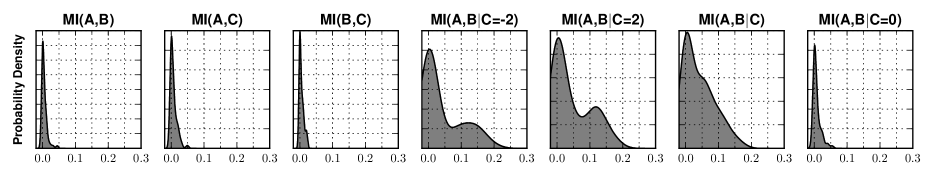
(b) The first three plots verify that $A$, $B$, and $C$ are marginally independent. The next three plots show that conditioning on $C$ “couples” the parents $A$ and $B$ (both for fixed values of $C\in\left\{{2,-2}\right\}$, and marginalizing over all $C$). The last plot shows that $\left\{{C=0}\right\}$ does not couple $A$ and $B$, due to symmetry of signum.

[width=]figures/common-graph

(c) Ground truth “common-cause” generator.

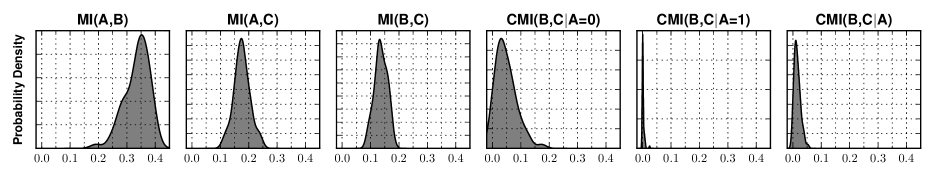
(d) The first three plots verify that $A$, $B$, and $C$ are marginally dependent. The next three plots show that conditioning on $A$ “decouples” the children $B$ and $C$; the decoupling is weaker for $\left\{{A=0}\right\}$, because it is 3.4 nats less likely that $\left\{{A=1}\right\}$. The final plot shows the weighted CMI under these two possibilities.

Figure 2: Posterior distributions of CMI under the DPMM posterior, given 100 data points from canonical Bayes net structures. Distributions peaked at 0 indicate high probability of (conditional) independence. In both cases, the posterior CMI distributions correctly detect the marginal, conditional, and context-specific independences in the “ground truth” Bayes nets, despite the fact that both “common-cause” and “common-effect” structures are not in the (structural) hypothesis space of the DPMM prior.

⬇

SIMULATE

MUTUAL INFORMATION OF

(x1, x2) WITH (x3)

GIVEN (x4 = 14)

FROM MODELS OF population

⬇

ESTIMATE PROBABILITY OF

MUTUAL INFORMATION OF

(x1, x2) WITH (x3)

GIVEN (x4 = 14, x5)

< 0.1

BY population

⬇

SIMULATE (

SELECT * FROM

VARIABLES OF population

WHERE PROBABILITY OF

MUTUAL INFORMATION

WITH x2 < 0.1

> 0.9)

FROM population

LIMIT 100;

1:for $\mathcal{G}_{k}\in\mathcal{M}$ do 2:  $\mathcal{I}_{\mathcal{G}_{k}}\leftarrow\textsc{Gpm-Cmi}(\mathcal{G}_{k},\left\{{x_{1},x_{2}}\right\},\left\{{x_{3}}\right\},\left\{{(x_{4},14)}\right\})$ 3:return $(\mathcal{I}_{\mathcal{G}_{1}},\dots,\mathcal{I}_{\mathcal{G}_{|\mathcal{M}|}})$ 1:for $\mathcal{G}_{k}\in\mathcal{M}$ do 2:  for $t=1,\dots,T$ do 3:   $\hat{x}_{5}^{t}\leftarrow\textsc{Simulate}(\mathcal{G}_{k},x_{5},\left\{{(x_{4},14)}\right\})$ 4:   $\mathcal{I}_{\mathcal{G}_{k}}^{t}\leftarrow\textsc{Gpm-Cmi}($ 5:     $\mathcal{G}_{k},\left\{{x_{1},x_{2}}\right\},\left\{{x_{3}}\right\},\left\{{(x_{4},14),(x_{5},\hat{x}_{5}^{t})}\right\})$    6:  $\mathcal{I}_{\mathcal{G}_{k}}\leftarrow\frac{1}{T}\sum_{t}\left(\mathcal{I}_{\mathcal{G}_{k}}^{t}\right)$ 7:return $\frac{1}{|\mathcal{M}|}\sum_{j}\left(\mathbb{I}\left[\mathcal{I}_{\mathcal{G}_{k}}<0.1\right]\right)$ 1:$\mathcal{S}\leftarrow\varnothing$ 2:for $x_{i}\in(x_{1},\dots,x_{D})$ do 3:  for $\mathcal{G}_{k}\in\mathcal{M}$ do 4:   $\mathcal{I}_{\mathcal{G}_{k}}\leftarrow\textsc{Gpm-Cmi}(\mathcal{G}_{k},x_{i},x_{2},\varnothing)$    5:  $p_{i}\leftarrow\frac{1}{|\mathcal{M}|}\sum_{k}{\mathbb{I}\left[\mathcal{I}_{\mathcal{G}_{k}}<0.1\right]}$ 6:  if $p_{i}>0.9$ then 7:   $\mathcal{S}\leftarrow\mathcal{S}\cup\left\{{x_{i}}\right\}$    8:for $t=1\dots,100$ do 9:  $s_{t}\leftarrow\textsc{Simulate}(\mathcal{M},\mathcal{S},\varnothing)$ 10:return $(s_{1},\dots,s_{100})$ English Summary of
CMI Query CMI Query in Bayesian Query Language Inference Algorithm Invoked by
Query Interpreter

 

Figure 3: End-user CMI queries in the Bayesian Query Language for three data analysis tasks; (top) evaluating the strength of predictive relationships; (middle) specifying the amount of evidence required for a “predictively” significant relationship; (bottom) synthesizing a hypothetical population, censoring probably sensitive variables.

Our approach to estimating the CMI requires a prior $\pi$ and model class $\mathcal{G}$ which is flexible enough to emulate an arbitrary joint distribution over $\bm{x}$, and tractable enough to implement Algorithm 2a for its arbitrary sub-vectors. We begin with a Dirichlet process mixture model (DPMM) [12]. Letting $L_{d}$ denote the likelihood for variable $d$, $V_{d}$ a prior over the parameters of $L_{d}$, and $\bm{\lambda}_{d}$ the hyperparameters of $V_{d}$, the generative process for $N$ observations $\mathscr{D}{=}\left\{{\bm{x}_{[i,1:D]}:1\leq i\leq N}\right\}$ is:

$$\underline{\textsc{DPMM-Prior}}$$

$$\alpha\sim\textsc{Gamma}(1,1)$$

$$\bm{z}=(z_{1},\dots,z_{N})\sim\textsc{CRP}(\cdot|\alpha)$$

$$\bm{\phi}_{[d,k]}\sim V_{d}(\cdot|\bm{\lambda}_{d}) d\in[D],k\in\textsc{Unique}(\bm{z})$$

$$x_{[i,d]}\sim L_{d}(\cdot|\bm{\phi}_{[d,z_{i}]}) i\in[N],d\in[D]$$

We refer to [7, 14] for algorithms for posterior inference, and assume we have a posterior sample $\hat{\mathcal{G}}=(\alpha,\bm{z}_{[1:N]},\left\{{\bm{\phi}_{d}}\right\})$ of all parameters in the DPMM. To compute the CMI of an arbitrary query pattern $\mathcal{I}_{\hat{\mathcal{G}}}(\bm{x}_{\mathcal{A}}{:}\bm{x}_{\mathcal{B}}|\bm{x}_{\mathcal{C}}{=}\hat{\bm{x}}_{\mathcal{C}})$ using Algorithm 2a, we need implementations of Simulate and LogPdf for $\hat{\mathcal{G}}$. These two procedures are summarized in Algorithms 3a, 3b.

Algorithm 3a DPMM-Simulate

1:DPMM $\mathcal{G}$; target $\mathcal{A}$; condition $\hat{\bm{x}}_{\mathcal{C}}$

2:joint sample $\hat{\bm{x}}_{\mathcal{A}}\sim p_{\mathcal{G}}(\cdot|\hat{\bm{x}}_{\mathcal{C}})$

3:$(l_{i})_{i=1}^{K+1}\leftarrow\textsc{DPMM-Cluster-Posterior}(\mathcal{G},\hat{\bm{x}}_{\mathcal{C}})$

4:$z_{N+1}\sim\textsc{Categorical}(l_{1},\dots,l_{K+1})$

5:for $a\in\mathcal{A}$ do

6:     $\hat{x}_{a}\sim L_{a}(\cdot|\bm{\phi}_{[a,z_{N+1}]})$

7:return $\hat{\bm{x}}_{\mathcal{A}}$

Algorithm 3b DPMM-LogPdf

1:DPMM $\mathcal{G}$; target $\hat{\bm{x}}_{\mathcal{A}}$; condition $\hat{\bm{x}}_{\mathcal{C}}$

2:log density $p_{\mathcal{G}}(\hat{\bm{x}}_{\mathcal{A}}|\hat{\bm{x}}_{\mathcal{C}})$

3:$(l_{i})_{i=1}^{K+1}\leftarrow\textsc{DPMM-Cluster-Posterior}(\mathcal{G},\hat{\bm{x}}_{\mathcal{C}})$

4:for $k=1,\dots,K+1$ do

5:     $t_{k}\leftarrow\prod_{a\in\mathcal{A}}L_{a}(\hat{x}_{a}|\bm{\phi}_{[a,k]})$

6:return $\log\left(\sum_{k=1}^{K+1}\left(t_{k}l_{k}\right)\right)$

Algorithm 3c DPMM-Cluster-Posterior

1:DPMM $\mathcal{G}$; condition $\hat{\bm{x}}_{\mathcal{C}}$;

2:$\left\{{p_{\mathcal{G}}(z_{N+1}=k):1\leq{k}\leq\max(\bm{z}_{1:N})+1}\right\}$

3:$K\leftarrow\max(\bm{z}_{1:N})$

4:for $k=1,\dots,K+1$ do

5:     $n_{k}\leftarrow\begin{cases}|\left\{{\bm{x}_{i}\in\mathscr{D}:z_{i}=k}\right\}|&\text{if }k\leq K\\ \alpha&\text{if }k=K+1\end{cases}$

6:     $l_{k}\leftarrow\left(\prod_{c\in\mathcal{C}}L_{c}(\hat{x}_{c}|\bm{\phi}_{[c,k]})\right)n_{k}$

7:return $(l_{1},\dots,l_{K+1})/\sum_{k=1}^{K+1}(l_{k})$

 

The subroutine DPMM-Cluster-Posterior is used for sampling (in DPMM-Simulate) and marginalizing over (in DPMM-LogPdf) the non-parametric mixture components. Moreover, if $L_{d}$ and $V_{d}$ form a conjugate likelihood-prior pair, then invocations of $L_{d}(\hat{x}_{d}|\bm{\phi}_{[d,k]})$ in Algorithms 3a:6 and 3b:5 can be Rao-Blackwellized by conditioning on the sufficient statistics of data in cluster $k$, thus marginalizing out $\bm{\phi}_{[d,k]}$ [26]. This optimization is important in practice, since analytical marginalization can be obtained in closed-form for several likelihoods in the exponential family [9]. Finally, to approximate the posterior distribution over CMI in (2), it suffices to aggregate DPMM-Cmi from a set of posterior samples $\left\{{\hat{\mathcal{G}}_{1},\dots,\hat{\mathcal{G}}_{H}}\right\}\sim^{\textrm{iid}}\pi(\cdot|\mathscr{D})$. Figure 2 shows posterior CMI distributions from the DPMM successfully recovering the marginal and conditional independencies in two canonical Bayesian networks.

3.1 Inducing sparse dependencies using the CrossCat prior

The multivariate DPMM makes the restrictive assumption that all variables $\bm{x}=(x_{1},\dots,x_{D})$ are (structurally) marginally dependent, where their joint distribution fully factorizes conditioned on the mixture assignment $z$. In high-dimensional datasets, imposing full structural dependence among all variables is too conservative. Moreover, while the Monte Carlo error of Algorithm 2a does not scale with the dimensionality $D$, its runtime scales linearly for the DPMM, and so estimating the CMI is likely to be prohibitively expensive. We relax these constraints by using CrossCat [19], a structure learning prior which induces sparsity over the dependencies between the variables of $\bm{x}$. In particular, CrossCat posits a factorization of $\bm{x}$ according to a variable partition $\bm{\gamma}=\left\{{\mathcal{V}_{1},\dots,\mathcal{V}_{|\bm{\gamma}|}}\right\}$, where $\mathcal{V}_{i}\subseteq[D]$. For $i\neq j$, all variables in block $\mathcal{V}_{i}$ are mutually (marginally and conditionally) independent of all variables in $\mathcal{V}_{j}$. The factorization of $\bm{x}$ given the variable partition $\bm{\gamma}$ is therefore given by:

$$p_{\mathcal{G}}(\bm{x}|\mathscr{D}) =\prod_{\mathcal{V}\in\bm{\gamma}}p_{\mathcal{G}_{\mathcal{V}}}(\bm{x}_{\mathcal{V}}|\mathscr{D}_{\mathcal{V}}).$$ (5)

Within block $\mathcal{V}$, the variables $\bm{x}_{\mathcal{V}}=\left\{{x_{d}:d\in\mathcal{V}}\right\}$ are distributed according to a multivariate DPMM; subscripts with $\mathcal{V}$ (such as $\mathcal{G}_{\mathcal{V}}$) now index a set of block-specific DPMM parameters. The joint predictive density $p_{\mathcal{G}_{\mathcal{V}}}$ is given by Algorithm 3b:

$$p_{\mathcal{G}_{\mathcal{V}}}(\bm{x}_{\mathcal{V}}|\mathscr{D})=\sum_{k=1}^{K_{V}+1}\left(\frac{n_{[\mathcal{V},k]}\prod\limits_{d\in\mathcal{V}}p_{\mathcal{G}_{\mathcal{V}}}(x_{d}|\bm{\phi}_{[d,k]})}{\sum_{k^{\prime}}n_{[\mathcal{V},k^{\prime}]}}\right).$$ (6)

The CrossCat generative process for $N$ observations $\mathscr{D}{=}\left\{{\bm{x}_{[i,1:D]}:1\leq i\leq N}\right\}$ is summarized below.

$$\underline{\textsc{CrossCat-Prior}}$$

$$\alpha^{\prime}\sim\textsc{Gamma}(1,1)$$

$$\bm{v}=(v_{1},\dots,v_{D})\sim\textsc{CRP}(\cdot|\alpha^{\prime})$$

$$\mathcal{V}_{k}\leftarrow\left\{{i\in[D]:v_{i}=k}\right\} k\in\textsc{Unique}(\bm{v})$$

$$\left\{{x_{[i,\mathcal{V}_{k}]}}\right\}_{i=1}^{N}\sim\textsc{DPMM-Prior} k\in\textsc{Unique}(\bm{v})$$

We refer to [19, 23] for algorithms for posterior inference in CrossCat, and assume we have a set of approximate samples $\left\{{\hat{\mathcal{G}}_{i}:1\leq i\leq H}\right\}$ of all latent CrossCat parameters from the posterior $\pi(\cdot|\mathscr{D})$.

3.2 Optimizing a CMI query

The following lemma shows how CrossCat induces sparsity for a multivariate CMI query.

Lemma 1.

Let $\mathcal{G}$ be a posterior sample from CrossCat, whose full joint distribution is given by (5) and (6). Then, for all $\mathcal{A},\mathcal{B},\mathcal{C}\subseteq[D]$,

$$\mathcal{I}_{\mathcal{G}}\left(\bm{x}_{\mathcal{A}}:\bm{x}_{\mathcal{B}}\mid\hat{\bm{x}}_{\mathcal{C}}\right)=\sum_{\mathcal{V}\in\bm{\gamma}}\mathcal{I}_{\mathcal{G}_{\mathcal{V}}}(\bm{x}_{\mathcal{A}\cap\mathcal{V}}:\bm{x}_{\mathcal{B}\cap\mathcal{V}}\mid\hat{\bm{x}}_{\mathcal{C}\cap\mathcal{V}}),$$

where $\mathcal{I}_{\mathcal{G}_{\mathcal{V}}}(\bm{x}_{\mathcal{A}\cap{\mathcal{V}}}:\varnothing|\hat{\bm{x}}_{\mathcal{C}\cap\mathcal{V}})\equiv 0$.

Proof.

Refer to Appendix A. ∎

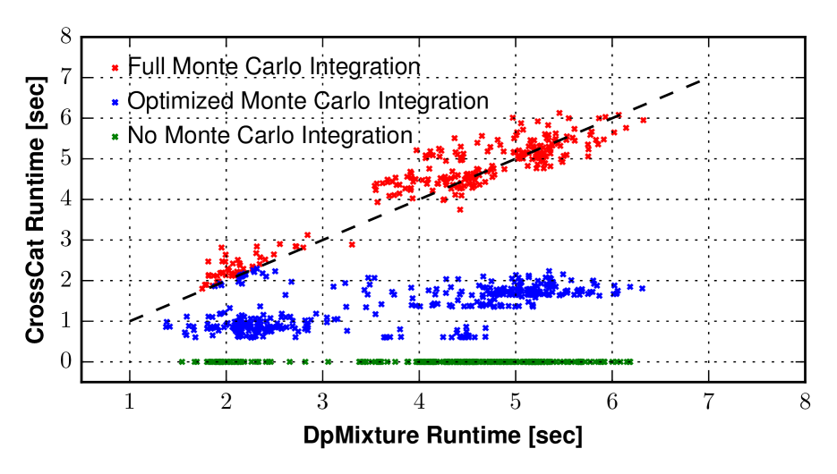
Figure 4: Comparing the runtime of CrossCat-Cmi (Alg 4a) and Gpm-Cmi (Alg 2a) (using the DPMM), on 1000 randomly generated CMI queries from an 8-dimensional dataset. The dashed curve shows the 45-degree line. The green dots at 0 correspond to CrossCat detecting structural independence between query variables, bypassing Monte Carlo estimation completely. The blue dots (below diagonal) correspond to CrossCat optimizing the Monte Carlo estimator by ignoring constraint variables which are structurally independent of the target variables. The red dots (along diagonal) correspond to CrossCat learning no structural independences, requiring full Monte Carlo estimation and resulting in comparable runtime to DPMM. These three cases correspond to the three posterior CrossCat structures illustrated in Figure 1, when the targets variables are $X$ and $Y$ conditioned on $W$.

 

An immediate consequence of Lemma 1 is that structure discovery in CrossCat allows us to optimize Monte Carlo estimation of $\mathcal{I}_{\mathcal{G}}(\bm{x}_{\mathcal{A}}:\bm{x}_{\mathcal{B}}|\bm{x}_{\mathcal{C}}=\hat{\bm{x}}_{\mathcal{C}})$ by ignoring all target and condition variables which are not in the same block $\mathcal{V}$, as shown in Algorithm 4a and Figure 4.

Algorithm 4a CrossCat-Cmi

1:CrossCat $\mathcal{G}$; query $\mathcal{A}$, $\mathcal{B}$; condition $\hat{\bm{x}}_{\mathcal{C}}$; acc. $T$

2:Monte Carlo estimate of $\mathcal{I}_{\mathcal{G}}(\bm{x}_{\mathcal{A}}{:}\bm{x}_{\mathcal{B}}|\bm{x}_{\mathcal{C}}{=}\hat{\bm{x}}_{\mathcal{C}})$

3:for $\mathcal{V}\in\bm{\gamma}$ do

4:  if  $\mathcal{A}\cap\mathcal{V}\;\;\textsc{and }\;\;\mathcal{B}\cap\mathcal{V}\ \textbf{then}$

5:   $i_{\mathcal{V}}\leftarrow$Gpm-Cmi($\mathcal{G}_{\mathcal{V}}$, $\mathcal{A}\cap\mathcal{V}$, $\mathcal{B}\cap\mathcal{V}$, $\hat{\bm{x}}_{\mathcal{C}{\cap}{\mathcal{V}}}$, $T$)

6:  else

7:   $i_{\mathcal{V}}\leftarrow 0$   

8:return $\sum_{\mathcal{V}\in\bm{\gamma}}i_{\mathcal{V}}$

3.3 Upper bounding the pairwise dependence probability

In exploratory data analysis, we are often interested in detecting pairwise predictive relationships between variables $(x_{i},x_{j})$. Using the formalism from Eq (3), we can compute the probability that their MI is non-zero: $\mathbb{P}\left[\mathcal{I}_{\mathcal{G}}(x_{i}:x_{j})>0\right]$. This quantity can be upper-bounded by the posterior probability that $x_{i}$ and $x_{j}$ have the same assignments $v_{i}$ and $v_{j}$ in the CrossCat variable partition $\bm{\gamma}$:

$$\mathbb{P}\left[\mathcal{I}_{\mathcal{G}}(x_{i}:x_{j})>0\right]$$

$$=\mathbb{P}\left[\mathcal{I}_{\mathcal{G}}(x_{i}:x_{j})>0\mid\left\{{\mathcal{G}:v_{i}=v_{j}}\right\}\right]\mathbb{P}\left[\left\{{\mathcal{G}:v_{i}=v_{j}}\right\}\right]$$

$$\;\;+\mathbb{P}\left[\mathcal{I}_{\mathcal{G}}(x_{i}:x_{j})>0\mid\left\{{\mathcal{G}:v_{i}\neq v_{j}}\right\}\right]\mathbb{P}\left[\left\{{\mathcal{G}:v_{i}\neq v_{j}}\right\}\right]$$

$$=\mathbb{P}\left[\mathcal{I}_{\mathcal{G}}(x_{i}:x_{j})>0\mid\left\{{\mathcal{G}:v_{i}=v_{j}}\right\}\right]\mathbb{P}\left[\left\{{\mathcal{G}:v_{i}=v_{j}}\right\}\right]$$

$$<\mathbb{P}\left[\left\{{\mathcal{G}:v_{i}=v_{j}}\right\}\right]\approx\frac{1}{H}\sum_{h=1}^{H}\mathbb{I}[\hat{\mathcal{G}}_{h}:\hat{v}_{[h,i]}=\hat{v}_{[h,j]}],$$ (7)

where Lemma 1 has been used to set the addend in line 3 to zero. Also note that the summand in (7) can be computed in $O(1)$ for CrossCat sample $\hat{\mathcal{G}}_{h}$. When dependencies among the $D$ variables are sparse such that many pairs $(x_{i},x_{j})$ have MI upper bounded by 0, the number of invocations of Algorithm 4a required to compute pairwise MI values is $\ll O(D^{2})$. A comparison of upper bounding MI versus exact MI estimation with Monte Carlo is shown in Figure 5.

Figure 5: Posterior probability that dimensions of a bivariate Gaussian are dependent, vs the covariance (top). The CrossCat upper bound (7) is useful for detecting the existence of a predictive relationship; the posterior distribution of MI can determine whether the strength of the relationship is “predictively significant” based on various tolerance levels (0.05, 0.10, 0.20, and 0.30 nats).

 

4 Applications to macroeconomic indicators of global poverty, education, and health

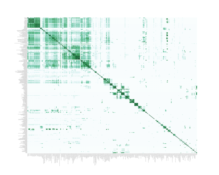
(a) $R^{2}$ Correlation Value

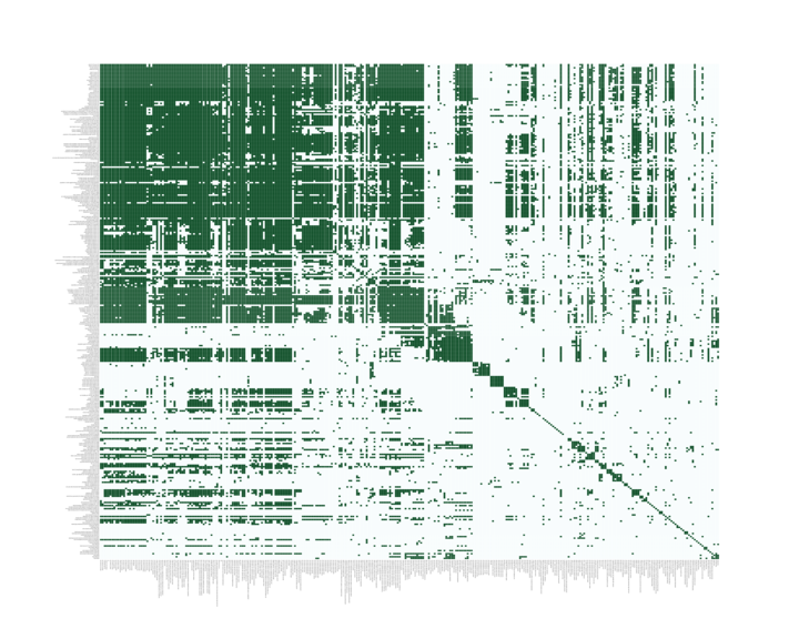
(b) HSIC [13] Independence Test

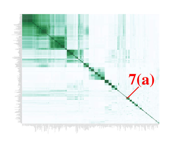
(c) $\mathbb{P}[\mathcal{I}_{\mathcal{G}}(x_{i}{:}x_{j})>0]$, Eq (7)

(d) Pairwise heatmaps of all 320 variables in the Gapminder dataset using three dependency detection techniques. Darker cells indicate a detected dependence between the two variables.

variable A	variable B	$\mathbb{P}[\mathcal{I}_{\mathcal{G}}>0]$	$R^{2}$ ($p\ll 10^{-6}$)
personal computers	earthquake affected	0.015625	0.974445
road traffic total deaths	people living w/ hiv	0.265625	0.858260
natural gas reserves	15-25 yrs sex ratio	0.031250	0.951471
forest products per ha	earthquake killed	0.046875	0.936342
flood affected	population 40-59 yrs	0.140625	0.882729

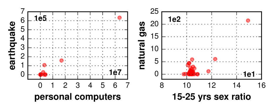
(a) Spurious relationships which are correlated under $R^{2}$, but probably independent according to posterior MI.

variable A	variable B	$\mathbb{P}[\mathcal{I}_{\mathcal{G}}>0]$	$R^{2}$ ($p\ll 10^{-6}$)
inflation	trade balance (% gdp)	0.859375	0.114470
DOTS detection rate	DOTS coverage	0.812500	0.218241
forest area (sq. km)	forest products (usd)	0.828125	0.206145
long term unemp. rate	total 15-24 unemp.	0.968750	NaN
male family workers	female self-employed	0.921875	NaN

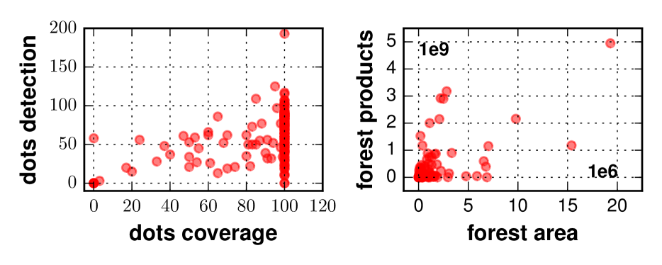
(a) Common-sense relationships probably dependent according to posterior MI, but weakly correlated under $R^{2}$.

Figure 9: Comparing dependences between variables in the Gapminder dataset, as detected by $R^{2}$, HSIC (with Bonferroni correction for multiple testing), and posterior distribution over mutual information in CrossCat.

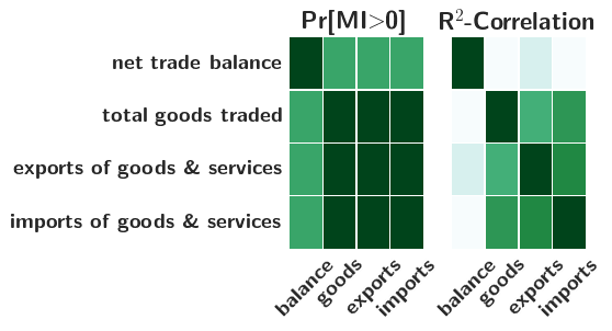
(a) Block of “trade” variables detected as probably dependent.

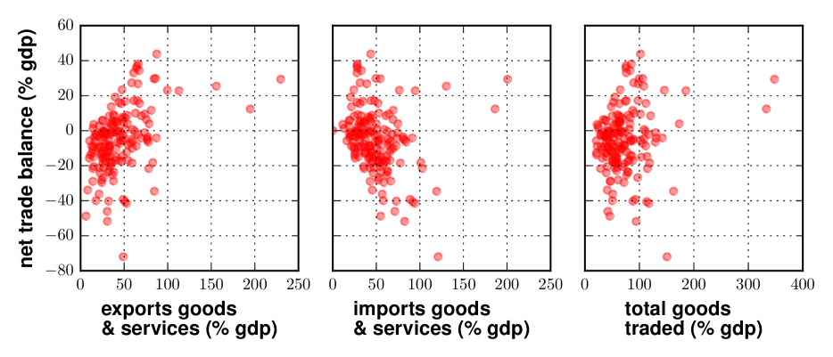
(b) Scatter plots show weak linear correlations and heteroskedastic noise for net balance.

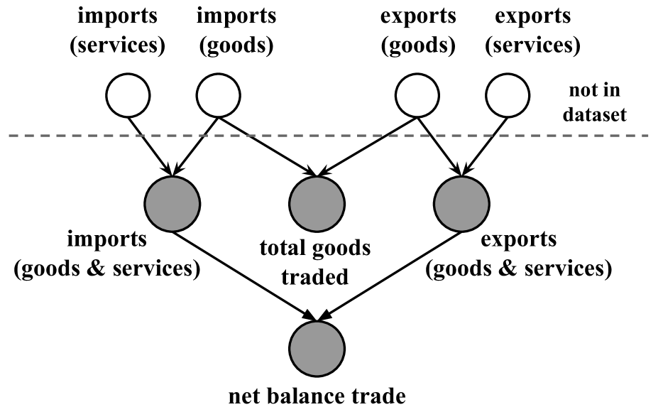
(c) Ground truth causal structure of variables in the “trade” block.

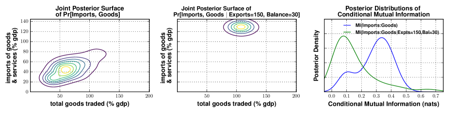
(d) Left plot shows the joint posterior density of “imports” and “goods”, where the marginal coupling is due to their common parent in 10(c). Center plot shows the same distribution conditioned on “exports”=150 and “balance”=30; “imports” now centers around its noiseless value of 120, and is decoupled from “goods”. Right plot shows the CMI for these distributions.

Figure 10: CMI discovers existence and confirms strength of predictive relationships between “trade” variables.

This section illustrates the efficacy of the proposed approach on a sparse database from an ongoing collaboration with the Bill & Melinda Gates Foundation. The Gapminder data set is an extensive longitudinal dataset of $\sim$320 global developmental indicators for 200 countries spanning over 5 centuries [27]. These include variables from a broad set of categories such as education, health, trade, poverty, population growth, and mortality rates. We experiment with a cross-sectional slice of the data from 2002. Figure 7(a) shows the pairwise $R^{2}$ correlation values between all variables; each row and column in the heatmap is an indicator in the dataset, and the color of a cell is the raw value of $R^{2}$ (between 0 and 1). Figure 7(b) shows pairwise binary hypothesis tests of independence using HSIC [13], which detects a dense set of dependencies including many spurious relationships (Appendix B). For both methods, statistically insignificant relationships ($\alpha=0.05$ with Bonferroni correction for multiple testing) are shown as 0. Figure 7(c) shows an upper bound on the pairwise probability that the MI of two variables exceeds zero (also a value between 0 and 1). These entries are estimated using Eq (7) (bypassing Monte Carlo estimation) using $H{=}100$ samples of CrossCat. Note that the metric $\mathbb{P}[\mathcal{I}_{\mathcal{G}}(x_{i}{:}x_{j})>0]$ in Figure 7(c) only indicates the existence of a predictive relationship between $x_{i}$ and $x_{j}$; it does not quantify either the strength or directionality of the relationship.

It is instructive to compare the dependencies detected by $R^{2}$ and CrossCat-Cmi. Table 8(a) shows pairs of variables that are spuriously reported as dependent according to correlation; scatter plots reveal they are either (i) are sparsely observed or (ii) exhibit high correlation due to large outliers. Table 9(a) shows common-sense relationships between pairs of variables that CrossCat-CMI detects but $R^{2}$ does not; scatter plots reveal they are either (i) non-linearly related, (ii) roughly linear with heteroskedastic noise, or (iii) pairwise independent but dependent given a third variable. Recall that CrossCat is a product of DPMMs; practically meaningful conditions for weak and strong consistency of Dirichlet location-scale mixtures have been established by [11, 33]. This supports the intuition that CrossCat can detect a broad class of predictive relationships that simpler parametric models miss.

Figure 10 focuses on a group of four “trade”-related variables in the Gapminder dataset detected as probably dependent: “net trade balance”, “total goods traded”, “exports of goods and services”, and “imports of goods and services”. $R^{2}$ fails to detect a statistically significant dependence between “net trade balance” and the other variables, due to weak linear correlations and heteroskedastic noise as shown in the scatter plots (Figure 10(b)). From economics, these four variables are causally related by the graphical model in Figure 10(c), where the value of a node is a noisy addition or subtraction of the values of its parents. Figure 10(d) illustrates that CrossCat recovers predictive relationships between these variables: conditioning on “exports”=150 and “balance”=30 (a low probability event according to the left subplot) centers the posterior predictive distribution of “imports” around 120, and decouples it from “total goods”. The posterior CMI curves of “imports” and “total goods”, with and without the conditions on “exports” and “balance”, formalize this decoupling (right subplot of Figure 10(d)).

5 Related Work

There is broad acknowledgment that new techniques for dependency detection beyond linear correlation are required. Existing approaches for conditional independence testing include the use of kernel methods [1, 10, 35, 29], copula functions [2, 25, 17], and characteristic functions [32], many of which capture non-linear and multivariate predictive relationships. Unlike these methods, however, our approach represents dependence in terms of conditional mutual information and is not embedded in a frequentist decision- theoretic framework. Our quantity of interest is a full posterior distribution over CMI, as opposed to a $p$-value to identify when the null hypothesis CMI=0 cannot be rejected. Dependence detection is much less studied in the Bayesian literature; [8] use a Polya tree prior to compute a Bayes Factor for the relative evidence of dependence versus independence. Their method is used only to quantify evidence for the existence, but not assess the strength, of a predictive relationship. The most similar approach to this work was proposed independently in recent work by [16], who compute a distribution over CMI by estimating the joint density using an encompassing non-parametric Bayesian prior. However, the differences are significant. First, the Monte Carlo estimator in [16] is based on resampling empirical data. However, real-world databases may be too sparse for resampling data to yield good estimates, especially for queries given unlikely constraints. Instead, we use a Monte Carlo estimator by simulating the predictive distribution. Second, the prior in [16] is a standard Dirichlet process mixture model, whereas this paper proposes a sparsity-inducing CrossCat prior, which permits optimized computations for upper bounds of posterior probabilities as well as simplifying CMI queries with multivariate conditions.

6 Discussion

This paper has shown it is possible to detect predictive relationships by integrating probabilistic programming, information theory, and non-parametric Bayes. Users specify a broad class of conditional mutual information queries using a simple SQL-like language, which are answered using a scalable pipeline based on approximate Bayesian inference. The underlying approach applies to arbitrary generative population models, including parametric models and other classes of probabilistic programs [28]; this work has focused on exploiting the sparsity of CrossCat model structures to improve scalability for exploratory analysis. With this foundation, one may extend the technique to domains such as causal structure learning. The CMI estimator can be used as a conditional-independence test in a structure discovery algorithm such as PC [31]. It is also possible to use learned CMI probabilities as part of a prior over directed acyclic graphs in the Bayesian setting. This paper has focused on detection and preliminary assessment of predictive relationships; confirmatory analysis and descriptive summarization are left for future work, and will require an assessment of the robustness of joint density estimation when random sampling assumptions are violated. Moreover, new algorithmic insights will be needed to scale the technique to efficiently detect pairwise dependencies in very high-dimensional databases with tens of thousands of variables.

Acknowledgements

This research was supported by DARPA (PPAML program, contract number FA8750-14-2-0004), IARPA (under research contract 2015-15061000003), the Office of Naval Research (under research contract N000141310333), the Army Research Office (under agreement number W911NF-13-1-0212), and gifts from Analog Devices and Google.

Appendix A Proof of optimizing a CMI query

Proof of Lemma 1.

We use the product-sum property of the logarithm (line 3) and linearity of expectation (line 4) to show that CrossCat’s variable partition $\bm{\gamma}$ induces a factorization of a CMI query.

$$\mathcal{I}_{\mathcal{G}}\left(\bm{x}_{\mathcal{A}}{:}\bm{x}_{\mathcal{B}}|\hat{\bm{x}}_{\mathcal{C}}\right)=\mathbb{E}\left[\log\left(\frac{p_{\mathcal{G}}(\bm{x}_{\mathcal{A}}{:}\bm{x}_{\mathcal{B}}|\hat{\bm{x}}_{\mathcal{C}})}{p_{\mathcal{G}}(\bm{x}_{\mathcal{A}}|\hat{\bm{x}}_{\mathcal{C}})p_{\mathcal{G}}(\bm{x}_{\mathcal{B}}|\hat{\bm{x}}_{\mathcal{C}})}\right)\right]$$

$$=\mathbb{E}\left[\log\left(\prod_{\mathcal{V}\in\bm{\gamma}}\frac{p_{\mathcal{G}_{\mathcal{V}}}(\bm{x}_{\mathcal{A}\cap\mathcal{V}},\bm{x}_{\mathcal{B}\cap\mathcal{V}}|\hat{\bm{x}}_{\mathcal{C}\cap\mathcal{V}})}{p_{\mathcal{G}_{\mathcal{V}}}(\bm{x}_{\mathcal{A}\cap\mathcal{V}}|\hat{\bm{x}}_{\mathcal{C}\cap\mathcal{V}})p_{\mathcal{G}_{\mathcal{V}}}(\bm{x}_{\mathcal{B}\cap\mathcal{V}}|\hat{\bm{x}}_{\mathcal{C}\cap\mathcal{V}})}\right)\right]$$

$$=\mathbb{E}\left[\sum_{\mathcal{V}\in\bm{\gamma}}\log\left(\frac{p_{\mathcal{G}_{\mathcal{V}}}(\bm{x}_{\mathcal{A}\cap\mathcal{V}},\bm{x}_{\mathcal{B}\cap\mathcal{V}}|\hat{\bm{x}}_{\mathcal{C}\cap\mathcal{V}})}{p_{\mathcal{G}_{\mathcal{V}}}(\bm{x}_{\mathcal{A}\cap\mathcal{V}}|\hat{\bm{x}}_{\mathcal{C}\cap\mathcal{V}})p_{\mathcal{G}_{\mathcal{V}}}(\bm{x}_{\mathcal{B}\cap\mathcal{V}}|\hat{\bm{x}}_{\mathcal{C}\cap\mathcal{V}})}\right)\right]$$

$$=\sum_{\mathcal{V}\in\bm{\gamma}}\mathbb{E}\left[\log\left(\frac{p_{\mathcal{G}_{\mathcal{V}}}(\bm{x}_{\mathcal{A}\cap\mathcal{V}},\bm{x}_{\mathcal{B}\cap\mathcal{V}}|\hat{\bm{x}}_{\mathcal{C}\cap\mathcal{V}})}{p_{\mathcal{G}_{\mathcal{V}}}(\bm{x}_{\mathcal{A}\cap\mathcal{V}}|\hat{\bm{x}}_{\mathcal{C}\cap\mathcal{V}})p_{\mathcal{G}_{\mathcal{V}}}(\bm{x}_{\mathcal{B}\cap\mathcal{V}}|\hat{\bm{x}}_{\mathcal{C}\cap\mathcal{V}})}\right)\right]$$

$$=\sum_{\mathcal{V}\in\bm{\gamma}}\mathcal{I}_{\mathcal{G}_{\mathcal{V}}}\left(\bm{x}_{\mathcal{A}\cap\mathcal{V}}{:}\bm{x}_{\mathcal{B}\cap\mathcal{V}}|\hat{\bm{x}}_{\mathcal{C}\cap\mathcal{V}}\right).$$

∎

Appendix B Experimental methods for dependence detection baselines

In this section we outline the methodology used to produce the pairwise $R^{2}$ and HSIC heatmaps shown in Figures 7(a) and 7(b). To detect the strength of linear correlation (for $R^{2}$) and perform a marginal independence test (for HSIC) given variables $x_{i}$ and $x_{j}$ in the Gapminder dataset, all records in which at least one of these two variables is missing were dropped. If the total number of remaining observations was less than three, the null hypothesis of independence was not rejected due to degeneracy of these methods at very small sample sizes. Hypothesis tests were performed at the $\alpha=0.05$ significance level. To account for multiple testing (a total of $\binom{320}{2}=51040$), a standard Bonferroni correction was applied to ensure a family-wise error rate of at most $\alpha$.

We used an open source MATLAB implementation for HSIC (function hsicTestBoot from http://gatsby.ucl.ac.uk/~gretton/indepTestFiles/indep.htm). 1000 permutations were used to approximate the null distribution, and kernel sizes were determined using median distances from the dataset. From Figure 7(b), HSIC detects a large number of statistically significant dependencies. Figures 12 and 12 report spurious relationships reported as dependent by HSIC but have a low dependence probability of less than 0.15 according to posterior CMI (Eq 7), and common-sense relationships reported as independent HSIC but have a high dependence probability.

Figure 11: Spurious relationships detected as dependent by HSIC ($p\ll 10^{-6}$) but probably independent ($\mathbb{P}[\mathcal{I}_{\mathcal{G}}(x_{i}{:}x_{j})>0]<0.15)$ by the MI upper bound.

variable A	variable B
body mass index (men)	privately owned forest (%)
energy use (per capita)	50+ yrs sex ratio
homicide (15-29)	inflation (annual %)
children out of primary school	male above 60 (%)
income share (fourth 20%)	suicide rate age 45-59
personal computers	arms exports (US$)
billionaires (per 1M)	mobile subscription (per 100)
residential elec. consumption	smear-positive detection (%)
coal consumption (per capita)	age at 1st marriage (women)
coal consumption (per capita)	dead kids per woman
underweight children	murder (per 100K)
female 0-4 years (%)	15+ literacy rate (%)
broadband subscribers (%)	dots new case detection (%)
crude oil prod. (per capita)	TB incidence (per 100K)
dependency ratio	people living with hiv

 

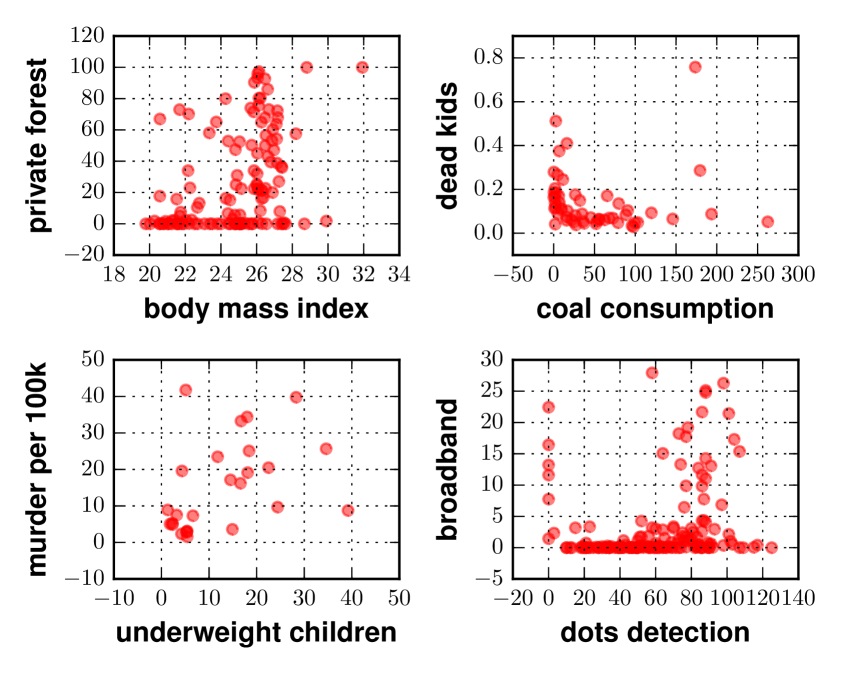
Figure 12: Common-sense relationships detected as independent by HSIC ($p\ll 10^{-6}$), but probably dependent ($\mathbb{P}[\mathcal{I}_{\mathcal{G}}(x_{i}{:}x_{j})>0]>0.85)$ by the MI upper bound.

variable A	variable B
motor vehicles per 1k	pop urban agglomerations (%)
car mortality (per 100K)	road incidents 45-59
wood removal (cubic m.)	primary forest land (ha)
forest products total (US$)	primary forest land (ha)
15-24 yrs sex ratio	50+ yrs sex ratio
gdp per working hr (US$)	urban population (%)
dots pop. coverage (%)	dots new case detection (%)
total 15-24 unemp. (%)	long term unemp. (%)
female self-employed (%)	female service workers (%)
female agricult. workers (%)	total industry workers (%)
female industry workers (%)	male industry workers (%)
road incidents age 60+	road incidents age 15-29
suicide rate age 15-29	suicide rate age 60+

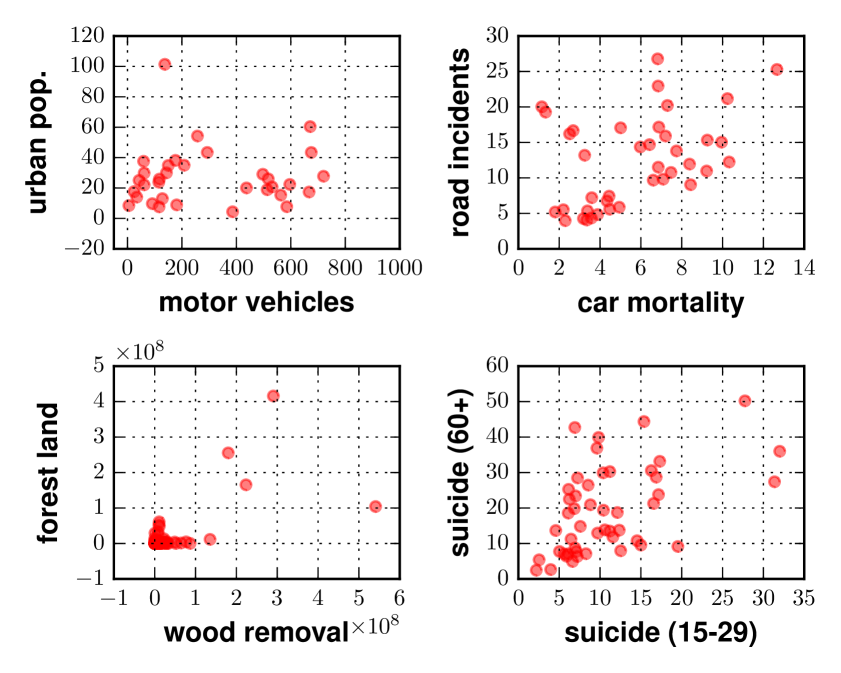
Appendix C Application to a database of mathematics marks

mech	vectors	algebra	analysis	stats
77	82	67	67	81
23	38	36	48	15
63	78	80	70	81
55	72	63	70	68
…	…	…	…	…

(a) Database of mathematics marks for 88 students, where rows are students and columns are exam scores.

	M	V	G	L	S
M	1.00	0.33	0.23	0.00	0.03
V	0.33	1.00	0.28	0.08	0.02
G	0.23	0.28	1.00	0.43	0.36
L	0.00	0.08	0.43	1.00	0.26
S	0.02	0.02	0.36	0.26	1.00

(b) Partial correlation matrix; red entries indicate statistically significant conditional independences.

(a) Undirected (Gaussian) graphical model implied by the partial correlation matrix.

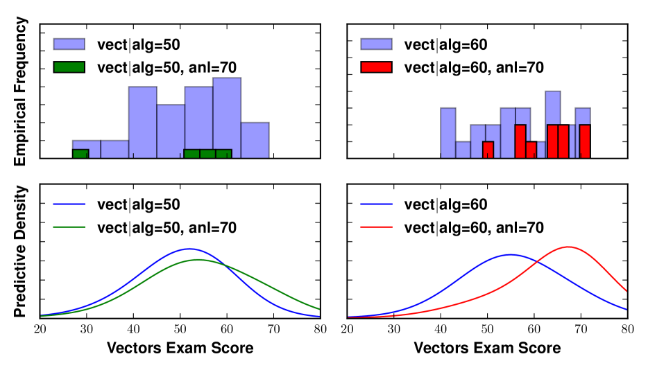
(b) Histograms from the raw dataset (top); and predictive distributions from CrossCat (bottom).

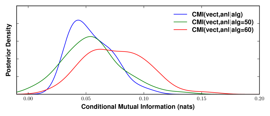
(c) Posterior distribution of CMI(vectors, analysis) given various conditions of algebra show context-specific dependence.

Figure 13: Using posterior CMI distributions to discover context-specific predictive relationships in the mathematics marks dataset [20, 34, 6] which are missed by partial correlations. 3(a) The database contains scores of 88 students on five mathematics exams: mechanics, vectors, algebra, analysis, and statistics. 3(b) Modeling the variables as jointly Gaussian and computing the partial correlation matrix indicates that (mechanics, vectors) are together conditionally independent of (analysis, statistics), given algebra. 13(a) A Gaussian graphical model which expresses the conditional independences relationships is formed by removing edges whose incident nodes have statistically-significant partial correlations of zero. The graph suggests that when predicting the vectors score for a student whose algebra score is known, further conditioning on the analysis score provides no additional information. We will critique this finding, by showing that the predictive strength of analysis on vectors given algebra varies, depending on the conditioning value of algebra. 13(b) The left panel shows that when algebra = 50, conditioning on analysis = 70 appears to have little effect on the prediction for vectors. The right panel shows that when algebra = 60, however, conditioning on analysis = 70 results in a sizeable shift of the posterior mean of vectors from 52 to just under 70. This shift is consistent with the top right histogram, where knowing that analysis = 70 eliminates all the vectors scores in the heavy left tail. 13(c) We formalize this “context-specific” dependence by computing the distribution of the CMI of vectors and analysis under two conditions: algebra = 50 (green curve), and algebra = 60 (red curve). The red curve places great probability on higher values of mutual information than the green curve, which explains the shift in predictive density from 13(b). Finally, we observe that the CMI is weakest when marginalizing over all values of algebra (blue curve), which explains why the partial correlation of vectors and analysis, which only considers marginal relationships, is near zero.

References

• Bach and Jordan [2002] Francis Bach and Michael Jordan. Kernel independent component analysis. Journal of Machine Learning Research, 3:1–48, 2002.
• Bouezmarni et al. [2012] Taoufik Bouezmarni, Jeroen VK Rombouts, and Abderrahim Taamouti. Nonparametric copula-based test for conditional independence with applications to granger causality. Journal of Business & Economic Statistics, 30(2):275–287, 2012.
• Boutilier et al. [1996] Craig Boutilier, Nir Friedman, Moises Goldszmidt, and Daphne Koller. Context-specific independence in bayesian networks. In Proceedings of the Twelfth International Conference on Uncertainty in Artificial Intelligence, pages 115–123. Morgan Kaufmann Publishers Inc., 1996.
• Council [2013] National Reseach Council. Frontiers in massive data analysis. The National Academies Press, 2013.
• Cover and Thomas [2012] T.M. Cover and J.A. Thomas. Elements of Information Theory. Wiley Series in Telecommunications and Signal Processing. Wiley, 2012.
• Edwards [2012] David Edwards. Introduction to graphical modelling. Springer Texts in Statistics. Springer, 2012.
• Escobar and West [1995] Michael Escobar and Mike West. Bayesian density estimation and inference using mixtures. Journal of the American Statistical Association, 90(430):577–588, 1995.
• Filippi and Holmes [2016] Sarah Filippi and Chris Holmes. A bayesian nonparametric approach to testing for dependence between random variables. Bayesian Analysis, 2016. Advance publication.
• Fink [1997] Daniel Fink. A compendium of conjugate priors. Technical report, Environmental Statistics Group, Department of Biology, Montana State University, 1997.
• Fukumizu et al. [2007] Kenji Fukumizu, Arthur Gretton, Xiaohai Sun, and Bernhard Schölkopf. Kernel measures of conditional dependence. In Proceedings of the Twentieth International Conference on Neural Information Processing Systems, pages 489–496. Curran Associates Inc., 2007.
• Ghosal et al. [1999] Subhashis Ghosal, Jayanta Ghosh, and R.V. Ramamoorthi. Posterior consistency of dirichlet mixtures in density estimation. The Annals of Statistics, 27(1):143–158, 1999.
• Görür and Rasmussen [2010] Dilan Görür and Carl Edward Rasmussen. Dirichlet process gaussian mixture models: Choice of the base distribution. Journal of Computer Science and Technology, 25(4):653–664, 2010.
• Gretton et al. [2005] Arthur Gretton, Olivier Bousquet, Alex Smola, and Bernhard Schölkopf. Measuring statistical dependence with hilbert-schmidt norms. In Proceedings of the Sixteenth International Conference Algorithmic Learning Theory, pages 63–77. Springer, 2005.
• Jain and Neal [2012] Sonia Jain and Radford M Neal. A split-merge markov chain monte carlo procedure for the dirichlet process mixture model. Journal of Computational and Graphical Statistics, 13(1):158–182, 2012.
• Kraskov et al. [2004] Alexander Kraskov, Harald Stögbauer, and Peter Grassberger. Estimating mutual information. Physical Review E, 69(6):066138, 2004.
• Kunihama and Dunson [2016] Tsuyoshi Kunihama and David B Dunson. Nonparametric bayes inference on conditional independence. Biometrika, 103(1):35–47, 2016.
• Lopez-Paz et al. [2013] David Lopez-Paz, Philipp Hennig, and Bernhard Schölkopf. The randomized dependence coefficient. In Proceedings of the Twenty-Sixth International Conference on Neural Information Processing Systems, pages 1–9. Curran Associates Inc., 2013.
• Mansinghka et al. [2015] Vikash Mansinghka, Richard Tibbetts, Jay Baxter, Pat Shafto, and Baxter Eaves. BayesDB: A probabilistic programming system for querying the probable implications of data. CoRR, abs/1512.05006, 2015.
• Mansinghka et al. [2016] Vikash Mansinghka, Patrick Shafto, Eric Jonas, Cap Petschulat, Max Gasner, and Joshua B. Tenenbaum. CrossCat: A fully Bayesian nonparametric method for analyzing heterogeneous, high dimensional data. Journal of Machine Learning Research, 17(138):1–49, 2016.
• Mardia et al. [1980] Kantilal Varichand Mardia, John T Kent, and John M Bibby. Multivariate analysis. Probability and Mathematical Statistics. Academic Press, 1980.
• Moddemeijer [1989] Rudy Moddemeijer. On estimation of entropy and mutual information of continuous distributions. Signal Processing, 16(3):233–248, 1989.
• Moon et al. [1995] Young-Il Moon, Balaji Rajagopalan, and Upmanu Lall. Estimation of mutual information using kernel density estimators. Physical Review E, 52(3):2318, 1995.
• Obermeyer et al. [2014] Fritz Obermeyer, Jonathan Glidden, and Eric Jonas. Scaling nonparametric Bayesian inference via subsample-annealing. In Proceedings of the Seventeenth International Conference on Artificial Intelligence and Statistics, pages 696–705. JMLR.org, 2014.
• Paninski [2003] Liam Paninski. Estimation of entropy and mutual information. Neural Computation, 15(6):1191–1253, 2003.
• Póczos et al. [2012] Barnabás Póczos, Zoubin Ghahramani, and Jeff Schneider. Copula-based kernel dependency measures. CoRR, abs/1206.4682, 2012.
• Robert and Casella [2005] Christian Robert and George Casella. Monte Carlo Statistical Methods. Springer Texts in Statistics. Springer, 2005.
• [27] Hans Rosling. Gapminder: Unveiling the beauty of statistics for a fact based world view. URL https://www.gapminder.org/data/.
• Saad and Mansinghka [2016] Feras Saad and Vikash Mansinghka. Probabilistic data analysis with probabilistic programming. CoRR, abs/1608.05347, 2016.
• Sejdinovic et al. [2013] Dino Sejdinovic, Arthur Gretton, and Wicher Bergsma. A kernel test for three-variable interactions. In Proceedings of the Twenty-Sixth International Conference on Neural Information Processing Systems, pages 1124–1132. Curran Associates Inc., 2013.
• Shachter [1998] Ross D Shachter. Bayes-ball: Rational pastime for determining irrelevance and requisite information in belief networks and influence diagrams. In Proceedings of the Fourteenth Conference on Uncertainty in Artificial Intelligence, pages 480–487. Morgan Kaufmann Publishers Inc., 1998.
• Spirtes et al. [2000] Peter Spirtes, Clark Glymour, and Richard Scheines. Causation, Prediction, and Search. Adaptive Computation and Machine Learning. MIT Press, 2000.
• Su and White [2007] Liangjun Su and Halbert White. A consistent characteristic function-based test for conditional independence. Journal of Econometrics, 141(2):807–834, 2007.
• Tokdar [2006] Surya T Tokdar. Posterior consistency of dirichlet location-scale mixture of normals in density estimation and regression. The Indian Journal of Statistics, 68(1):90–110, 2006.
• Whittaker [1990] Joe Whittaker. Graphical models in applied multivariate statistics. Wiley Series in Probability and Mathematical Statistics. Wiley, 1990.
• Zhang et al. [2011] Kun Zhang, Jonas Peters, and Dominik Janzing. Kernel-based conditional independence test and application in causal discovery. In Proceedings of the Twenty-Seventh Conference on Uncertainty in Artificial Intelligence, pages 804–813. AUAI Press, 2011.