A New Track Reconstruction Algorithm suitable for Parallel Processing based on Hit Triplets and Broken Lines

Abstract

Track reconstruction in high track multiplicity environments at current and future high rate particle physics experiments is a big challenge and very time consuming. The search for track seeds and the fitting of track candidates are usually the most time consuming steps in the track reconstruction. Here, a new and fast track reconstruction method based on hit triplets is proposed which exploits a three-dimensional fit model including multiple scattering and hit uncertainties from the very start, including the search for track seeds. The hit triplet based reconstruction method assumes a homogeneous magnetic field which allows to give an analytical solutions for the triplet fit result. This method is highly parallelizable, needs fewer operations than other standard track reconstruction methods and is therefore ideal for the implementation on parallel computing architectures. The proposed track reconstruction algorithm has been studied in the context of the Mu3e-experiment and a typical LHC experiment.

1 Introduction

Track reconstruction in high energy experiments at high luminosity colliders is a big challenge. The large particle rates together with the track extrapolation uncertainties, generated by multiple Coulomb scattering in the silicon tracking detector material, lead to hit confusion and define the hit combinatorial problem. High track multiplicities not only increase considerably the computational effort for solving this combinatorial problem, they also reduce the track finding efficiency and purity.

Standard track reconstruction algorithms employed in high track multiplicity environments consist typically of the following steps:

• Seed search: A minimum number of hits in several tracking layers is required to form a track seed. For the reconstruction of initial track parameters at least three points are required. This could be hits in three detector layers or in only two detector layers if additional constraints on the origin of the track, e.g. collision point, are employed.

• Fitting of track prototypes and seeds: By using a tracking model, which ideally should include spatial hit uncertainties as well as multiple scattering uncertainties, track parameters of seeds and prototypes are determined.

• Hit linking: Using previously fitted track parameters, the particle trajectory of the track prototype is extrapolated to link hits from further detector layers. Track extrapolation uncertainties are usually included by defining a search window. Hit linking is terminated if hits in all tracking layers are found or no further hits can be found because of missing hits.

• Fit quality: Track candidates have to fulfill some quality criteria, that is a minimum number of linked hits (layers), minimum track length, minimum track fit quality, etc.

• Arbitration between track candidates: Different track candidates can share one or several hits. An arbitration algorithm can be used to find the “best” track candidate. Other track candidates sharing the same hits are discarded.

The steps 2 and 3 are iterated until all hits are linked or no more track candidates can be found. The Kálmán filter Kalman:1960:nal ; Fruhwirth:1987:akf ; BilloirEtAl:1990:spr is an example for such an iterative algorithm which is used as standard tool for track reconstruction in many particle physics experiments.

Besides track fitting the most time consuming step is usually the track seed finding due to the hit combinatorics. For a track seed search in $n_{layer}$ layers the processing time scales with $(N_{\rm hit})^{n_{layer}}$ where $N_{\rm hit}$ is the number of hits. For this reason track seed searches are often performed in regions of low occupancies (i.e. outer tracking layers in case of collider experiments). Different methods can be used to further reduce the hit combinatorial problem in the track seed search in the successive hit linking step:

• application of simple geometrical preselection cuts,

• application of more advanced algorithms like cellular automata Abt:2002he ,

• Hough transforms ref:Hough ,

• usage of lookup tables or associative memories.

Here, a new method is proposed for solving the hit combinatorial problem for seed finding and linking of hits to tracks. It can be used to accelerate the steps 1 – 4 in comparison with other standard reconstruction algorithms. The proposed method is based on hit triplets for which the track parameters can be instantly calculated by exploiting a three-dimensional fit model including multiple scattering and hit uncertainties. This fit requires the three-dimensional hit coordinates including their uncertainties and is only applicable in homogeneous magnetic fields. Both requirements are usually fulfilled in modern pixel tracking devices.

2 Method

Figure 1: Sketch of merging hit triplets to full tracks. The track fit result of each triplet is given by the three-dimensional radius $R_{3D}$, its uncertainty $\sigma(R_{3D})$ and the fit quality $\chi^{2}$.

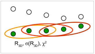
The hit triplet based track reconstruction method works as follows. In a first step hit triplets are found by fitting three-hit combinations and by applying a $\chi^{2}$-cut on the triplet fit quality. What is new compared with other similar methods is here the full exploitation of the tracking model at this very first track reconstruction step, thus reducing the number of wrong seeds and mitigating the combinatorial problem. As this method is rigorous it also works for “large triplets” with far distant hits and large track curvatures. After having found valid hit triplets, conjoined triplets (triplets which share two hits) are merged successively to full tracks, see Figure 1. The resulting trajectory is finally represented by broken lines. The track parameters are combined using a simple and fast sum which is explained in more detail in Section 3. This fast summing technique is much faster than other reconstruction methods which are based on iterations and rely on matrix inversions. Furthermore, the fast summing technique is exact if multiple scattering uncertainties dominate, being the case for the majority of particles at hadron colliders if silicon tracking detectors are used.

Above described merging technique only includes local but no long-range hit correlations which are important for the reconstruction of high momentum tracks. For high momentum tracks spatial hit uncertainties dominate over multiple scattering uncertainties and a global fit is required. This can be realized by applying a General Broken Line Fit (GBL) Blobel:2006:nft ; BlobelEtAl:2011:fac ; Kleinwort:2012:gbl after triplet merging. The GBL fit is an extended track fit that takes into account both, scattering effects and spatial uncertainties, and has been shown Kleinwort:2012:gbl to be equivalent to the Kálmán filter Fruhwirth:1987:akf . The GBL algorithm performs a linearized fit by varying positions and kink angles at selected points around a reference trajectory, which is here chosen to be the merged triplet trajectory.

2.1 Fitting of Hit Triplets

The most general objective function for track fitting includes multiple scattering and spatial hit uncertainties

$$\chi^{2}\ =\ \frac{\Theta_{MS}^{2}}{\sigma_{\theta}^{2}}+\frac{\Phi_{MS}^{2}}{\sigma_{\phi}^{2}}+\sum_{jk}({\bf x_{j}}-{\bf\xi_{j}}){\bf V^{-1}_{jk}}({\bf x_{k}}-{\bf\xi_{k}})\ .$$

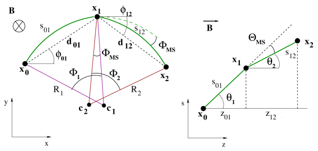
Here, $\Phi_{MS}$ and $\Theta_{MS}$ are the multiple scattering uncertainties in the transverse and longitudinal plane, see Figure 2. ${\bf x_{k}}$ and ${\bf\xi_{k}}$ are the fitted and measured hit coordinates and ${\bf V}$ is the covariance matrix.

For a particle moving in a homogeneous magnetic field an analytical solution can be calculated for a trajectory measured at three points (hit triplet). The solution for the case of negligible spatial hit uncertainties is briefly summarized in the next section (for a full description see ref:triplet_paper ). The solution for including spatial hit uncertainties is discussed in the following Section 2.1.2.

Figure 2: Particle trajectory in a homogeneous magnetic field defined by a triplet of hits $\mathbf{x_{0}}$, $\mathbf{x_{1}}$ and $\mathbf{x_{2}}$. The left view shows the projection to the plane transverse to the magnetic field, whereas the right view is a projection to the field axis-arclength ($s$) plane. $\Phi_{MS}$ and $\Theta_{MS}$ denote the multiple scattering angles in the transverse and longitudinal plane.

2.1.1 Triplet Fit with Multiple Scattering

If spatial uncertainties are negligible, i.e. ${\bf x_{k}}={\bf\xi_{k}}$, the right side of Equation 2.1 can be neglected. Assuming energy conservation the fit has one degree of freedom. The multiple scattering angles projected in the transverse and longitudinal plane can then be written as a function of the three-dimensional radius $\Phi_{MS}=\Phi_{MS}(R_{3D})$ and $\Theta_{MS}=\Theta_{MS}(R_{3D})$ which in turn is related to the momentum $p$ of the particle via $R_{3D}=p/(qB)$ with $q$ being the electric charge. $\Phi_{MS}(R_{3D})$ and $\Theta_{MS}(R_{3D})$ are transcendent functions which can not be algebraically solved. However, the minimization condition

$$\frac{{d}}{{d}R_{{3D}}}\chi^{2}(R_{{3D}})=0$$

can be solved by linearization around the circle solution in the transverse plane which is described in detail in ref:triplet_paper . The result for the three-dimensional radius

$$R_{{3D}}=-\;\frac{\eta\;\tilde{\Phi}_{C}\;\sin^{2}{\vartheta_{C}}+\beta\;\tilde{\Theta}_{C}}{\eta^{2}\;\sin^{2}{\vartheta_{C}}+\beta^{2}}\quad$$ (1)

depends only on parameters derived from the relative position of the hit coordinates, $\eta,\tilde{\Phi}_{C},\beta,\tilde{\Theta}_{C}=f({\bf x_{k}})$, and the polar angle $\vartheta_{C}$ which can be approximated from the circle solution. The exact definitions of these geometric parameters can be found in ref:triplet_paper . The corresponding uncertainty is given by

$$\sigma({R_{3D}})\ =\ \sigma_{MS}\;\sqrt{\frac{1}{\eta^{2}\;\sin^{2}{\vartheta_{C}}+\beta^{2}}}$$

and contains the expected multiple scattering uncertainty, which can be calculated using the Highland approximation Highland:1975:prm

$$\sigma_{MS}\approx\frac{13.6\leavevmode\nobreak\ \textrm{MeV/c}}{\beta p}\sqrt{X/X_{0}}$$ (2)

after fitting, using the effective material thickness $X$ at the middle hit position where the scattering takes place. Finally the fit quality is given by

$$\chi_{min}^{2}=\frac{1}{\sigma_{MS}^{2}}\ \frac{(\beta\;\tilde{\Phi}_{C}-\eta\;\tilde{\Theta}_{C})^{2}}{\eta^{2}+\beta^{2}/\sin^{2}{\vartheta_{C}}}\ .$$

2.1.2 Triplet Fit with Hit Uncertainties

In case of non-negligible spatial hit uncertainties the above description yields too large $\chi^{2}$-values and will fail. For hit triplets this bias can be fixed elegantly by absorbing the hit uncertainties in the scattering angles. By introducing effective scattering angles

$${\Delta}\Theta\ =\ \Theta_{\rm MS}+\Theta_{\rm hit}\quad\textrm{and}\quad{\Delta}\Phi\ =\ \Phi_{\rm MS}+\Phi_{\rm hit}\ ,$$

a new objective function can be defined

$$\chi^{2}\ =\ \frac{{\Delta}\Theta^{2}}{{\sigma_{\theta}}^{2}_{\textrm{eff}}}+\frac{{\Delta}\Phi^{2}}{{\sigma_{\phi}^{2}}_{\textrm{eff}}},$$

where effective hit uncertainties have been introduced

$${\sigma_{\theta}^{2}}_{\textrm{eff}}=\sigma_{\rm MS}^{2}+\sigma_{\theta_{hit}}^{2}\quad\textrm{and}\quad{\sigma_{\Phi}^{2}}_{\textrm{eff}}=\frac{\sigma_{\rm MS}^{2}}{\sin^{2}{\vartheta_{C}}}+\sigma_{\Phi_{hit}}^{2}.\quad$$

The hit-related uncertainties $\sigma_{\theta_{hit}}$ and $\sigma_{\Phi_{hit}}$ are obtained by propagating the uncertainties from the hit positions, see Appendix A. Note that this simplified procedure does not fit the hit positions, i.e. ${\bf x_{k}}={\bf\xi_{k}}$, but it yields the correct $\chi^{2}$-distribution, i.e. the probability distribution is flat. This is essential to validate the hit triplets for the track reconstruction.

Figure 3: Representation of hit uncertainty modes of a hit triplet. From left to right: curvature uncertainty, shift uncertainty and rotation uncertainty.

Finally, the three-dimensional radius is obtained by calculating:

$$R_{\rm{3D}}^{min}=-\;\frac{\eta\;\tilde{\Phi}_{\rm C}\sin{\vartheta_{C}}^{2}/\sigma_{\phi}(R_{\rm{3D}}^{min})^{2}+\beta\;\tilde{\Theta}_{\rm C}/\sigma_{\theta}(R_{\rm{3D}}^{min})^{2}}{\eta^{2}\sin{\vartheta_{C}}^{2}/\sigma_{\phi}(R_{\rm{3D}}^{min})^{2}+\beta^{2}/\sigma_{\theta}(R_{\rm{3D}}^{min})^{2}}.$$

By using the Highland approximation (Equation 2) above equation can be transformed into a cubic equation in $R_{\rm{3D}}^{min}$ which is algebraically solvable, see Appendix C.

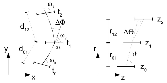
The inclusion of the hit uncertainties generates nine extra degrees of freedom. Relevant for track fitting and reconstruction are only six , which can be represented as “triplet bending”, “triplet shifting” and “triplet rotation” in the transverse as well as in the longitudinal plane, see Figure 3. The triplet bending is included in above fitting procedure, whereas shifts and rotations of the hit triplet are not. For track extrapolations, however, they might be relevant and have to be included. The rotational uncertainty of a hit triplet is given in Appendix B.

3 Triplet Linking and Merging

For the linking of hit triplets (or between a validated triplet and a track prototype) two strategies can be employed, the intersection technique and the extrapolation technique. In the intersection technique hits shared between validated triplets are used to identify connected tracks, see Figure 1. This can be done quickly in hardware by using fast lookup techniques or in software by using binary search trees, for example.

The extrapolation technique extrapolates already reconstructed track prototypes or triplets into other detector layers to add new single hits or hit triplets. This method is very efficient if the search window is small. That is typically the case for long track prototypes for which the track parameters have been precisely fitted in the previous step. Both techniques can also be combined to speed up linking.

The consistency of a new track hypothesis can be tested by calculating a combined $\chi^{2}_{comb}$ value by summing over all contributing triplets, where the number of hit triplets given is by $n_{hit}-2$. There is some freedom in how to perform the weighting in the sum. For dominating multiple scattering uncertainties and if the $R_{\rm{3D},i}$ were calculated using Equation 1 the optimal sum reads:

$$\chi_{comb}^{2}=\sum_{i}^{n_{hit}-2}\chi_{i}^{2}\ +\ \frac{(R_{\rm{3D},i}-\overline{R_{\rm{3D}}})^{2}}{\sigma_{i}(\overline{R_{3D}})^{2}}$$ (3)

with

$$\overline{R_{3D}}=\sum_{i}^{n_{hit}-2}\frac{R_{3D,i}^{2}}{\sigma(R_{3D,i})^{2}}\;\big{/}\;\sum_{i}^{n_{hit}-2}\frac{R_{3D,i}}{\sigma(R_{3D,i})^{2}}.$$ (4)

This definition of the averaged three-dimensional radius is free of bias. Equations 3 and 4 are exact and no refitting of the track parameters after the linking step is required.

For dominating hit uncertainties, the relative momentum resolution is no longer constant and it is advantageous to perform the $\chi^{2}$ sum and the averaging in three-dimensional curvature, $h_{3D}=1/R_{3D}$, yielding:

$$\chi_{comb}^{2}=\sum_{i}^{n_{hit}-2}\chi_{i}^{2}\ +\ \frac{(h_{3D,i}-\overline{h_{3D}})^{2}}{\sigma_{i}(\overline{h_{3D}})^{2}}$$ (5)

with

$$\overline{h_{3D}}=\sum_{i}^{n_{hit}-2}\frac{h_{3D,i}}{\sigma(h_{3D,i})^{2}}\;\big{/}\;\sum_{i}^{n_{hit}-2}\frac{1}{\sigma(h_{3D,i})^{2}}.$$ (6)

Equations 5 and 6 are not exact since long range correlations are ignored and triplet parameter uncertainties are overestimated in the procedure described in Section 2.1.2. The so obtained combined $\chi^{2}$ value is only a lower (optimistic) estimate. However, this combination procedure is very fast, highly parallelizable and useful for track fitting as it allows to quickly reject wrong triplet combinations without refitting.

The full precision is finally obtained by fitting, in addition to the kink angles, the hit positions ${\bf x}$, see next section.

4 General Broken Line Fit

Figure 4: Track parameter resolution for an equidistant layer geometry of a high energy LHC-type detector as described in ref:triplet_paper . The top panel shows the relative momentum resolution and the bottom panels show the resolution of the azimuthal angle $\phi$ and the polar angle $\vartheta$ for tracks with a polar angle of $\vartheta=70^{\circ}$. Plot taken from ref:triplet_paper .

Long-range correlations among different hit triplets can be included by the GBL fit Blobel:2006:nft ; BlobelEtAl:2011:fac ; Kleinwort:2012:gbl . It performs a linearization around a reference trajectory which is here chosen to be the broken line solution discussed in the previous section. A GBL fit using the triplets fit as reference has been recently implemented in Kiehn2016 ; Watson .

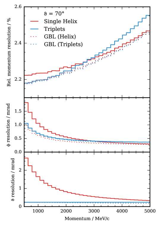
The performance of this fit and the improvement with respect to the triplets fit solution and a solution obtained from a single helix fit has been studied in ref:triplet_paper for a typical high energy LHC detector with equidistant layer spacing. The track parameter resolutions obtained by the different track fits for particles at $\vartheta=70^{\circ}$ are shown in Figure 4 for the momentum, azimuthal angle and polar angle. In the momentum range up to about $2$ GeV/c the triplets fit provides a resolution which is equally good as the GBL fits. In this region the triplet fit is considered to be adequate. Note that more than 99% of all charged particles produced at the LHC have a transverse momentum below $1$ GeV.

In the momentum range of above $2$ GeV/c the track parameter resolutions is significantly improved by using the GBL fit. For even higher momenta $p\geq 5$ GeV/c a single helix fit can be applied which requires far less computational effort than the GBL fit. The combination of the triplets fit for low momenta and a single helix fit for high momenta provide a very efficient scheme for fast track reconstruction. Only in the intermediate regime between about $2$ to $5$ GeV/c significant performance improvements are possible by using the GBL fit.

The triplet based track reconstruction method has been successfully implemented for the Mu3e-experiment RP ; Berger:2013raa and tested in simulations. The Mu3e-experiment will search for the lepton flavor violating decay of stopped muons $\mu^{+}\rightarrow e\leavevmode\nobreak\ ^{+}e\leavevmode\nobreak\ ^{+}e\leavevmode\nobreak\ ^{-}$. Because of the very low momentum of the decay electrons tracking is performed in kinematic region which is dominated by multiple scattering and spatial hit uncertainties can be ignored. For the Mu3e-experiment the above described track reconstruction based on hit triplets was successfully implemented on GPUs.

Triplet based tracking was also implemented for an upgraded ATLAS detector designed for High Luminosity LHC. It was successfully tested for different detector geometries and different layer spacings. A publication of the results is foreseen in the near future.

5 Summary and Outlook

A new track reconstruction method based on hit triplets has been proposed. It is based on a multiple scattering based track model ref:triplet_paper which has been extended here to include also spatial hit uncertainties. The described triplet fit has an algebraic solution and can be used to quickly validate hit combinations. It is therefore ideally suited for track reconstruction in general, and track seed searches in particular. The proposed method gives a simple prescription for the combination of hit triplets. The fit quality and the track momentum can be represented by sums, which can be quickly calculated. This method can be easily combined with a General Broken Line Fit to improve the track parameters for non-vanishing spatial hit uncertainties. For high momentum tracks (negligible multiple scattering) a single helix fit can be used alternatively, which is much faster than the GBL fit.

The whole track reconstruction procedure is non-iterative. All hit triplets can be reconstructed in parallel, what makes it ideal for the implementation on parallel computing architectures.

The used tracking model relies on the assumption that the magnetic field within a triplet is homogeneous and that multiple scattering occurs only at or near the detection layers. The effect of non-homogeneous magnetic fields, particles with missing hits in layers due to detector efficiencies, and particle scattering in material outside the detection layers will be subject of further studies.

Appendix A Propagation of Triplet Hit Uncertainties

Figure 5: Hit triplet with spatial hit uncertainties and definition of the kink angle uncertainties in the transverse (left) and longitudinal (right) plane.

A simple method to include hit uncertainties in the triplet fit is to interpret the hit residuals as kink angles: $\Delta\Phi$ in the transverse and $\Delta\Theta$ in the longitudinal plane, see Figure 5. The tilt angles with respect to the particle trajectory are given by the angles $\omega_{i}$. The uncertainties in radial direction ${\sigma_{r_{k}}}$, in azimuthal direction ${\sigma_{t_{k}}}$ and in axial direction ${\sigma_{z_{k}}}$ can be propagated to define effective kink angle uncertainties $\sigma_{\phi_{hit}}$ and $\sigma_{\theta_{hit}}$:

$$\sigma_{\phi_{hit}}^{2} =\frac{\sin^{2}{\omega_{0}}}{\Delta d_{01}^{2}}\;\sigma_{t_{0}}^{2}\;+\;\frac{\sin^{2}{\omega_{3}}}{\Delta d_{12}^{2}}\;\sigma_{t_{2}}^{2}\;+\;\left(\frac{\sin{\omega_{1}}}{\Delta d_{01}}+\frac{\sin{\omega_{2}}}{\Delta d_{12}}\right)^{2}\sigma_{t_{1}}^{2}$$

$$+\frac{\cos^{2}{\omega_{0}}}{\Delta d_{01}^{2}}\;\sigma_{r_{0}}^{2}\;+\;\frac{\cos^{2}{\omega_{3}}}{\Delta d_{12}^{2}}\;\sigma_{r_{2}}^{2}\;+\;\left(\frac{\cos{\omega_{1}}}{\Delta d_{01}}+\frac{\cos{\omega_{2}}}{\Delta d_{12}}\right)^{2}\sigma_{r_{1}}^{2}$$ (7)

$$\sigma_{\theta_{hit}}^{2} =\sin^{4}{\vartheta}\;\left(\frac{\sigma_{z_{0}}^{2}}{\Delta r_{01}^{2}}+\frac{\sigma_{z_{2}}^{2}}{\Delta r_{12}^{2}}+\sigma_{z_{1}}^{2}\;\left(\frac{1}{\Delta r_{01}}+\frac{1}{\Delta r_{12}}\right)^{2}\right)$$

$$+\sin^{2}{\vartheta}\;\cos^{2}{\vartheta}\;\left(\frac{\sigma_{r_{0}}^{2}}{\Delta r_{01}^{2}}+\frac{\sigma_{r_{2}}^{2}}{\Delta r_{12}^{2}}+\sigma_{r_{1}}^{2}\;\left(\frac{1}{\Delta r_{01}}+\frac{1}{\Delta r_{12}}\right)^{2}\right)\ .$$

Appendix B Triplet Rotation Uncertainty

For non-vanishing spatial hit uncertainties rotational degrees of freedom in the transverse and in the longitudinal plane are generated. These rotational uncertainties are important for track extrapolations. For a barrel-type detector and negligible track curvatures the rotational uncertainties are given by:

$$\delta\theta_{rot}^{2} =\sin^{4}{\vartheta}\;\;\frac{\sigma_{z_{0}}^{2}\sigma_{z_{1}}^{2}+\sigma_{z_{1}}^{2}\sigma_{z_{2}}^{2}+\sigma_{z_{0}}^{2}\sigma_{z_{2}}^{2}}{\sigma_{z_{0}}^{2}r_{12}^{2}+\sigma_{z_{2}}^{2}r_{01}^{2}+\sigma_{z_{1}}^{2}r_{02}^{2}}$$

$$\delta\phi_{rot}^{2} =\frac{\sigma_{t_{0}}^{2}\sigma_{t_{1}}^{2}+\sigma_{t_{1}}^{2}\sigma_{t_{2}}^{2}+\sigma_{t_{0}}^{2}\sigma_{t_{2}}^{2}}{\sigma_{t_{0}}^{2}d_{12}^{2}+\sigma_{t_{2}}^{2}d_{01}^{2}+\sigma_{t_{1}}^{2}d_{02}^{2}}.$$

Here the same notation as in Appendix A is used. It is straight-forward to calculate the rotational uncertainties for other detector orientations.

Appendix C Extended Triplet Fit with Hit Uncertainties

The three-dimensional radius in an extended triplet fit including hit uncertainties is given by:

$$R_{{3D}}^{min} =-\;\frac{\eta\;\tilde{\Phi}_{C}\sin{\vartheta}^{2}/\sigma_{\phi}(R_{{3D}}^{min})^{2}+\beta\;\tilde{\Theta}_{C}/\sigma_{\theta}(R_{{3D}}^{min})^{2}}{\eta^{2}\sin{\vartheta}^{2}/\sigma_{\phi}(R_{{3D}}^{min})^{2}+\beta^{2}/\sigma_{\theta}(R_{{3D}}^{min})^{2}}.$$

The polar angle of the track $\vartheta$ can be taken from the circle solution, which also can serve as a first estimate to calculate the inclination angles $\omega_{i}$ in the transverse plane, see Figure 5. Note that in general $\sigma_{\phi}\neq\sigma_{\theta}$.

A difficulty arises from the fact that the multiple scattering uncertainty depends on the particle momentum, which is not known before track fitting. A solution is to include this momentum dependence in the fit by using the Highland parameterization (Equation 2), leading to the following cubic equation:

$$0 ={R_{{3D}}^{min}}^{3}\;(\eta^{2}\sigma_{\theta_{hit}}^{2}+\beta^{2}\sigma_{\phi_{hit}}^{2})$$

$$+{R_{{3D}}^{min}}^{2}\;(\eta\;\tilde{\Phi}_{C}\;\sigma_{\theta_{hit}}^{2}+\beta\;\tilde{\Theta}_{C}\;\sigma_{\phi_{hit}}^{2})$$

$$+R_{{3D}}^{min}\;b^{2}\;(\eta^{2}+\beta^{2}/\sin{\vartheta}^{2})$$

$$+b^{2}\;(\eta\;\tilde{\Phi}_{C}+\beta\;\tilde{\Theta}_{C}/\sin{\vartheta}^{2})$$

$$:=a_{3}{R_{{3D}}^{min}}^{3}+a_{2}{R_{{3D}}^{min}}^{2}+a_{1}{R_{{3D}}^{min}}+a_{0}.$$

Here $b$ is an effective scattering parameter, which is a measure for the material thickness at the scattering layer, see ref:triplet_paper for definition. Using Cardano’s formula it is straight forward to find the solution for $R_{{3D}}^{min}$.

References

- (1) R.E. Kalman, J. Basic Eng. 82, 35 (1960)
- (2) R. Frühwirth, Nucl. Instr. Meth. A 262, 444 (1987)
- (3) P. Billoir, S. Qian, Nucl. Instr. Meth. A 294, 219 (1990)
- (4) I. Abt, D. Emelyanov, I. Kisel, S. Masciocchi, Nucl. Instrum. Meth. A489, 389 (2002)
- (5) P. Hough, U.S. Patent 3,069,654 (1962)
- (6) V. Blobel, Nucl. Instr. Meth. A 566, 14 (2006)
- (7) V. Blobel, C. Kleinwort, F. Meier, Comput. Phys. Commun. 182, 1760 (2011)
- (8) C. Kleinwort, Nucl. Instr. Meth. A 673, 107 (2012)
- (9) N. Berger, M. Kiehn, A. Kozlinskyi, A. Schöning, submitted to Nucl. Instr. Meth. A (2016), 1606.04990
- (10) V.L. Highland, Nucl. Instr. Meth. A 129, 497 (1975)
- (11) M. Kiehn, Ph.D. thesis, Physics Institute, Heidelberg University (Februar 2016)
- (12) M. Kiehn, WATSON A Tracking Library, internal software, University Heidelberg
- (13) A. Blondel et al., arXiv e-prints (2013), 1301.6113
- (14) N. Berger et al., Nucl. Instr. Meth. A 732, 61 (2013), 1309.7896