Perturbative QCD and beyond: azimuthal angle correlations in deuteron-deuteron scattering from Bose-Einstein correlations.

E.  Gotsman gotsman@post.tau.ac.il Department of Particle Physics, School of Physics and Astronomy, Raymond and Beverly Sackler Faculty of Exact Science, Tel Aviv University, Tel Aviv, 69978, Israel    E.  Levin leving@post.tau.ac.il, eugeny.levin@usm.cl Department of Particle Physics, School of Physics and Astronomy, Raymond and Beverly Sackler Faculty of Exact Science, Tel Aviv University, Tel Aviv, 69978, Israel Departemento de Física, Universidad Técnica Federico Santa María, and Centro Científico-
Tecnológico de Valparaíso, Avda. Espana 1680, Casilla 110-V, Valparaíso, Chile
Abstract

In this paper, we found within the framework of perturbative QCD, that in deuteron-deuteron scattering the Bose-Einstein correlations due to two parton showers production, induce azimuthal angle correlations, with three correlation lengths: the size of the deuteron (RDsubscript𝑅𝐷R_{D}), the proton radius (RNsubscript𝑅𝑁R_{N}), and the size of the BFKL Pomeron which, is closely related to the saturation momentum (Rc1/Qssimilar-tosubscript𝑅𝑐1subscript𝑄𝑠R_{c}\sim 1/Q_{s}). These correlations are independent of the values of rapidities of the produced gluons (long range rapidity correlations), for large rapidities (α¯S|y1y2|1subscript¯𝛼𝑆subscript𝑦1subscript𝑦21\bar{\alpha}_{S}|y_{1}-y_{2}|\geq 1), and have no symmetry with respect to ϕπϕitalic-ϕ𝜋italic-ϕ\phi\to\pi-\phi (𝒑T1𝒑T1subscript𝒑𝑇1subscript𝒑𝑇1\boldsymbol{p}_{T1}\to-\boldsymbol{p}_{T1}). Therefore, they give rise to vnsubscript𝑣𝑛v_{n} for all values of n𝑛n, not only even values. The contributions with the correlation length RDsubscript𝑅𝐷R_{D} and RNsubscript𝑅𝑁R_{N} crucially depend on the non-perturbative contributions, and to obtain estimates of their values, requiries a lot of modeling, while the correlations with Rc1/Qssimilar-tosubscript𝑅𝑐1subscript𝑄𝑠R_{c}\sim 1/Q_{s} have a perturbative QCD origin, and can be estimated in the Color Glass Condensate (CGC) approach.

BFKL Pomeron, soft interaction, CGC/saturation approach, correlations
pacs:
12.38.-t,24.85.+p,25.75.-q
preprint: TAUP-3007/16

I Introduction

In this paper we continue to resurrect the old ideas of Gribov Pomeron Calculus, that the Bose -Einstein correlations lead to strong azimuthal angle correlationsPION , which do not depend on the rapidity difference between measured hadrons ( large range rapidity (LRR) correlations). In the framework of QCD, these azimuthal correlations stem from the production of two patron showers, and have been re-discovered in Refs.KOWE ; KOLUCOR . In Ref.GLMBE it was demonstrated that Bose–Einstein correlations generate vnsubscript𝑣𝑛v_{n} with even and odd n𝑛n, with values which are close to the experimental values CMSPP ; STARAA ; PHOBOSAA ; STARAA1 ; CMSPA ; CMSAA ; ALICEAA ; ALICEPA ; ATLASPP ; ATLASPA ; ATLASAA .

The goal of this paper is to show that the Bose–Einstein correlations that have been discussed in Refs.PION ; GLMBE , arise naturally in the perturbative QCD approach, together with ones that have been considered in Refs.KOWE ; KOLUCOR . We believe that the qualitative difference between these two approaches originates from different sources of the Bose-Einstein correlations: the two parton shower production in Refs.PION ; GLMBE and one parton shower for Refs.KOWE ; KOLUCOR .

We consider here the azimuthal correlations for deuteron-deuteron scattering at high energy. It is well knownHBT , (see also Refs. IPCOR ) that Bose-Einstein correlations provide a possibility to measure the volume of interaction or, in other words, the typical sizes of the interaction. Indeed, the general formula for the Bose-Einstein correlations HBT ; IPCOR takes the form

d2σdy1dy2d2pT1d2pT2(identicalgluons)1+eirμQμproportional-tosuperscript𝑑2𝜎𝑑subscript𝑦1𝑑subscript𝑦2superscript𝑑2subscript𝑝𝑇1superscript𝑑2subscript𝑝𝑇2identicalgluonsdelimited-⟨⟩1superscript𝑒𝑖subscript𝑟𝜇subscript𝑄𝜇\frac{d^{2}\sigma}{dy_{1}\,dy_{2}d^{2}p_{T1}d^{2}p_{T2}}\left(\rm identical\,\,gluons\right)\,\,\propto\,\,\Big{\langle}1\,\,+\,\,e^{ir_{\mu}Q_{\mu}}\Big{\rangle} (1)

where averaging delimited-⟨⟩\langle\dots\rangle includes the integration over rμ=r1,μr2,μsubscript𝑟𝜇subscript𝑟1𝜇subscript𝑟2𝜇r_{\mu}=r_{1,\mu}-r_{2,\mu}. For the case of y1=y2subscript𝑦1subscript𝑦2y_{1}=y_{2}, Qμ=p1,μp2,μsubscript𝑄𝜇subscript𝑝1𝜇subscript𝑝2𝜇Q_{\mu}=p_{1,\mu}\,-\,p_{2,\mu} simplifies to 𝑸𝒑T,12=𝒑T1𝒑T2𝑸subscript𝒑𝑇12subscript𝒑𝑇1subscript𝒑𝑇2\boldsymbol{Q}\,\equiv\,\boldsymbol{p}_{T,12}\,=\,\boldsymbol{p}_{T1}\,-\,\boldsymbol{p}_{T2},

One can see that Eq. (1) allows us to measure the typical rμsubscript𝑟𝜇r_{\mu} for the interaction. For deuteron-deuteron scattering we expect several typical r𝑟r: the size of the deuteron RDsubscript𝑅𝐷R_{D}, the nucleon size RNsubscript𝑅𝑁R_{N}, and the typical size, related to the saturation scale (rsat=1/Qssubscript𝑟sat1subscript𝑄𝑠r_{\rm sat}\,=1/Q_{s}, where Qssubscript𝑄𝑠Q_{s} denotes the saturation scaleKOLEB ). In our calculation we hope to see the appearance of these scales.

It is well known, that the total cross section for the deuteron-deuteron scattering can be written in the form: σDD= 4σNNΔσDDsubscript𝜎𝐷𝐷4subscript𝜎𝑁𝑁Δsubscript𝜎𝐷𝐷\sigma_{DD}\,=\,4\sigma_{NN}\,-\,\Delta\sigma_{DD}, where ΔσDDΔsubscript𝜎𝐷𝐷\Delta\sigma_{DD} is the Glauber correction termGLA which is proportional to 1/RD21subscriptsuperscript𝑅2𝐷1/R^{2}_{D}, while σNNsubscript𝜎𝑁𝑁\sigma_{NN} denotes the total cross section of the nucleon-nucleon interaction. Intuition, suggests that the correlation radius of the order of RDsubscript𝑅𝐷R_{D}, stems from the production due to the Glauber correction term (see Fig. 1)

Refer to caption
Figure 1: The two parton showers production that contributes to the Glauber correction term for deuteron-deuteron scattering. The wavy lines describe the exchange of the BFKL Pomeron. Fig. 1-a and Fig. 1-b show two diagrams that can interfer for identical gluons. The dashed lines show the cut BFKL Pomeron AGK .

The production of two gluon are shown in Fig. 1-a and Fig. 1-b, where interference in the case of the generated identical gluon leads to the correlation function of Eq. (1). Generally speaking, the inclusive production of two gluons with rapidities y1subscript𝑦1y_{1} and y2subscript𝑦2y_{2} and transverse momenta 𝒑T1subscript𝒑𝑇1\boldsymbol{p}_{T1} and 𝒑T2subscript𝒑𝑇2\boldsymbol{p}_{T2}, takes the form

d2σdy1dy2d2pT1d2pT2(identicalgluons)=superscript𝑑2𝜎𝑑subscript𝑦1𝑑subscript𝑦2superscript𝑑2subscript𝑝𝑇1superscript𝑑2subscript𝑝𝑇2identicalgluonsabsent\displaystyle\frac{d^{2}\sigma}{dy_{1}\,dy_{2}d^{2}p_{T1}d^{2}p_{T2}}\left(\rm identical\,\,gluons\right)\,\,= (2)
d2σdy1dy2d2pT1d2pT2(differentgluons)(1squaredofdiagrams+C(Rc|𝒑T1𝒑T2|)interferencediagram)superscript𝑑2𝜎𝑑subscript𝑦1𝑑subscript𝑦2superscript𝑑2subscript𝑝𝑇1superscript𝑑2subscript𝑝𝑇2differentgluonssubscript1squaredofdiagramssubscript𝐶subscript𝑅𝑐subscript𝒑𝑇1subscript𝒑𝑇2interferencediagram\displaystyle\frac{d^{2}\sigma}{dy_{1}\,dy_{2}d^{2}p_{T1}d^{2}p_{T2}}\left(\rm different\,\,gluons\right)\,\Bigg{(}\underbrace{1}_{\rm squared\,of\,diagrams}\,\,\,+\,\,\underbrace{C\left(R_{c}|\boldsymbol{p}_{T1}\,-\,\boldsymbol{p}_{T2}|\right)}_{\rm interference\,diagram}\Bigg{)}

In Eq. (2) Rcsubscript𝑅𝑐R_{c} denotes the correlation radius (correlation length), and in the form of the correlation function, we anticipate that the production of two parton showers leads to the double inclusive cross section, that does not depend on rapidities y1subscript𝑦1y_{1} and y2subscript𝑦2y_{2}.

II Born Approximation

II.1 Bose-Einstein correlation function with radius 𝑹𝑫proportional-toabsentsubscript𝑹𝑫\propto\,\,R_{D}

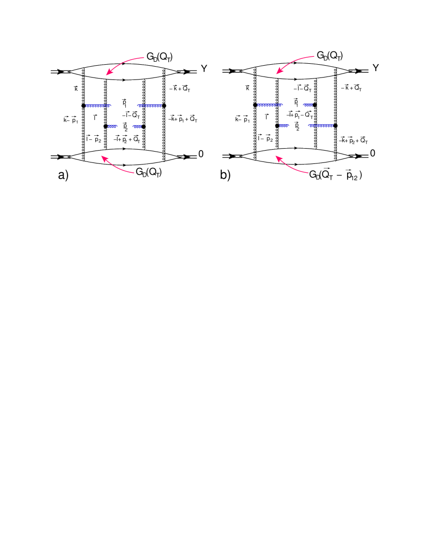
The simplest contribution in the Born approximation of perturbative QCD is shown in Fig. 2. The second diagram describes the interference between two parton showers, shown in Fig. 1-b.
Refer to caption
Figure 2: The double inclusive production of two gluons with rapidities y1subscript𝑦1y_{1} and y2subscript𝑦2y_{2} and transverse momenta 𝒑T1subscript𝒑𝑇1\boldsymbol{p}_{T1} and 𝒑T2subscript𝒑𝑇2\boldsymbol{p}_{T2}, in the Born Approximation of perturbative QCD. The interference diagram of Fig. 2-b gives the correlation function C(RD|𝒑T1𝒑T2|)𝐶subscript𝑅𝐷subscript𝒑𝑇1subscript𝒑𝑇2C\left(R_{D}|\boldsymbol{p}_{T1}\,-\,\boldsymbol{p}_{T2}|\right) of Eq. (2). The solid lines denote nucleons in the deuterons, which are specified by double lines

The analytical expressions take the following forms. For the diagram of Fig. 2-a we have

d2σdy1dy2d2pT1d2pT2(Fig.2a)d2QTGD2(QT)\displaystyle\frac{d^{2}\sigma}{dy_{1}\,dy_{2}d^{2}p_{T1}d^{2}p_{T2}}\left({Fig.~{}\ref{ddba}}-a\right)\,\,\propto\,\int d^{2}Q_{T}G^{2}_{D}\left(Q_{T}\right) (3)
×\displaystyle\times d2ktd2lT(IP(𝒌T,𝒌T+𝑸T)𝒌T2(𝒌𝒑1)T2Γμ(𝒌T,𝒑T1)Γμ(𝒌T+𝑸T,𝒑T1)IP(𝒌T𝒑T1,𝒌T+𝒑T1+𝑸T)(𝒌+𝑸)T2(𝒌+𝒑1+𝑸)T2)superscript𝑑2subscript𝑘𝑡superscript𝑑2subscript𝑙𝑇subscript𝐼𝑃subscript𝒌𝑇subscript𝒌𝑇subscript𝑸𝑇subscriptsuperscript𝒌2𝑇subscriptsuperscript𝒌subscript𝒑12𝑇subscriptΓ𝜇subscript𝒌𝑇subscript𝒑𝑇1subscriptΓ𝜇subscript𝒌𝑇subscript𝑸𝑇subscript𝒑𝑇1subscript𝐼𝑃subscript𝒌𝑇subscript𝒑𝑇1subscript𝒌𝑇subscript𝒑𝑇1subscript𝑸𝑇subscriptsuperscript𝒌𝑸2𝑇subscriptsuperscript𝒌subscript𝒑1𝑸2𝑇\displaystyle\int d^{2}k_{t}\,d^{2}l_{T}\Bigg{(}\frac{I_{P}\left(\boldsymbol{k}_{T},-\boldsymbol{k}_{T}+\boldsymbol{Q}_{T}\right)}{\boldsymbol{k}^{2}_{T}\,\left(\boldsymbol{k}-\boldsymbol{p}_{1}\right)^{2}_{T}}\Gamma_{\mu}\left(\boldsymbol{k}_{T},\boldsymbol{p}_{T1}\right)\,\Gamma_{\mu}\left(-\boldsymbol{k}_{T}+\boldsymbol{Q}_{T},\boldsymbol{p}_{T1}\right)\,\frac{I_{P}\left(\boldsymbol{k}_{T}-\boldsymbol{p}_{T1},-\boldsymbol{k}_{T}+\boldsymbol{p}_{T1}+\boldsymbol{Q}_{T}\right)}{\left(-\boldsymbol{k}+\boldsymbol{Q}\right)^{2}_{T}\,\left(-\boldsymbol{k}+\boldsymbol{p}_{1}+\boldsymbol{Q}\right)^{2}_{T}}\,\Bigg{)}
×\displaystyle\times (IP(𝒍T,𝒍T𝑸T)𝒍T2(𝒍𝒑2)T2Γν(𝒍T,𝒑T2)Γν(𝒍T𝑸T,𝒑T2)IP(𝒍T𝒑T2,𝒍T+𝒑T2𝑸T)(𝒍𝑸)T2(𝒍+𝒑2𝑸)T2)subscript𝐼𝑃subscript𝒍𝑇subscript𝒍𝑇subscript𝑸𝑇subscriptsuperscript𝒍2𝑇subscriptsuperscript𝒍subscript𝒑22𝑇subscriptΓ𝜈subscript𝒍𝑇subscript𝒑𝑇2subscriptΓ𝜈subscript𝒍𝑇subscript𝑸𝑇subscript𝒑𝑇2subscript𝐼𝑃subscript𝒍𝑇subscript𝒑𝑇2subscript𝒍𝑇subscript𝒑𝑇2subscript𝑸𝑇subscriptsuperscript𝒍𝑸2𝑇subscriptsuperscript𝒍subscript𝒑2𝑸2𝑇\displaystyle\Bigg{(}\frac{I_{P}\left(\boldsymbol{l}_{T},-\boldsymbol{l}_{T}-\boldsymbol{Q}_{T}\right)}{\boldsymbol{l}^{2}_{T}\,\left(\boldsymbol{l}-\boldsymbol{p}_{2}\right)^{2}_{T}}\Gamma_{\nu}\left(\boldsymbol{l}_{T},\boldsymbol{p}_{T2}\right)\,\Gamma_{\nu}\left(-\boldsymbol{l}_{T}-\boldsymbol{Q}_{T},\boldsymbol{p}_{T2}\right)\,\frac{I_{P}\left(\boldsymbol{l}_{T}-\boldsymbol{p}_{T2},-\boldsymbol{l}_{T}+\boldsymbol{p}_{T2}-\boldsymbol{Q}_{T}\right)}{\left(-\boldsymbol{l}-\boldsymbol{Q}\right)^{2}_{T}\,\left(-\boldsymbol{l}+\boldsymbol{p}_{2}-\boldsymbol{Q}\right)^{2}_{T}}\,\Bigg{)}

The interference diagram of Fig. 2-b takes the following form

d2σdy1dy2d2pT1d2pT2(Fig.2b)d2QTGD(QT)GD(𝑸T+𝒑T,12)\displaystyle\frac{d^{2}\sigma}{dy_{1}\,dy_{2}d^{2}p_{T1}d^{2}p_{T2}}\left({Fig.~{}\ref{ddba}}-b\right)\,\,\propto\,\int d^{2}Q_{T}G_{D}\left(Q_{T}\right)\,G_{D}\left(\boldsymbol{Q}_{T}\,+\,\boldsymbol{p}_{T,12}\right) (4)
×\displaystyle\times d2kTd2lT(IP(𝒌T,𝒌T+𝑸T)𝒌T2(𝒌𝒑1)T2Γμ(𝒌T,𝒑T1)Γμ(𝒍T𝑸T,𝒑T1)IP(𝒌T𝒑T1,𝒌T+𝒑T1+𝑸T)(𝒍𝑸)T2(𝒍+𝒑1𝑸)T2)superscript𝑑2subscript𝑘𝑇superscript𝑑2subscript𝑙𝑇subscript𝐼𝑃subscript𝒌𝑇subscript𝒌𝑇subscript𝑸𝑇subscriptsuperscript𝒌2𝑇subscriptsuperscript𝒌subscript𝒑12𝑇subscriptΓ𝜇subscript𝒌𝑇subscript𝒑𝑇1subscriptΓ𝜇subscript𝒍𝑇subscript𝑸𝑇subscript𝒑𝑇1subscript𝐼𝑃subscript𝒌𝑇subscript𝒑𝑇1subscript𝒌𝑇subscript𝒑𝑇1subscript𝑸𝑇subscriptsuperscript𝒍𝑸2𝑇subscriptsuperscript𝒍subscript𝒑1𝑸2𝑇\displaystyle\int d^{2}k_{T}\,d^{2}l_{T}\Bigg{(}\frac{I_{P}\left(\boldsymbol{k}_{T},-\boldsymbol{k}_{T}+\boldsymbol{Q}_{T}\right)}{\boldsymbol{k}^{2}_{T}\,\left(\boldsymbol{k}-\boldsymbol{p}_{1}\right)^{2}_{T}}\Gamma_{\mu}\left(\boldsymbol{k}_{T},\boldsymbol{p}_{T1}\right)\,\Gamma_{\mu}\left(-\boldsymbol{l}_{T}-\boldsymbol{Q}_{T},\boldsymbol{p}_{T1}\right)\,\frac{I_{P}\left(\boldsymbol{k}_{T}-\boldsymbol{p}_{T1},-\boldsymbol{k}_{T}+\boldsymbol{p}_{T1}+\boldsymbol{Q}_{T}\right)}{\left(-\boldsymbol{l}-\boldsymbol{Q}\right)^{2}_{T}\,\left(-\boldsymbol{l}+\boldsymbol{p}_{1}-\boldsymbol{Q}\right)^{2}_{T}}\,\Bigg{)}
×\displaystyle\times (IP(𝒍T,𝒍T𝑸T)𝒍T2(𝒌𝒑2)T2Γμ(𝒍T,𝒑T2)Γμ(𝒌T+𝑸T,𝒑T2)IP(𝒍T𝒑T2,𝒍T+𝒑T2𝑸T)(𝒌+𝑸)T2(𝒌+𝒑2+𝑸)T2)subscript𝐼𝑃subscript𝒍𝑇subscript𝒍𝑇subscript𝑸𝑇subscriptsuperscript𝒍2𝑇subscriptsuperscript𝒌subscript𝒑22𝑇subscriptΓ𝜇subscript𝒍𝑇subscript𝒑𝑇2subscriptΓ𝜇subscript𝒌𝑇subscript𝑸𝑇subscript𝒑𝑇2subscript𝐼𝑃subscript𝒍𝑇subscript𝒑𝑇2subscript𝒍𝑇subscript𝒑𝑇2subscript𝑸𝑇subscriptsuperscript𝒌𝑸2𝑇subscriptsuperscript𝒌subscript𝒑2𝑸2𝑇\displaystyle\Bigg{(}\frac{I_{P}\left(\boldsymbol{l}_{T},-\boldsymbol{l}_{T}-\boldsymbol{Q}_{T}\right)}{\boldsymbol{l}^{2}_{T}\,\left(\boldsymbol{k}-\boldsymbol{p}_{2}\right)^{2}_{T}}\Gamma_{\mu}\left(\boldsymbol{l}_{T},\boldsymbol{p}_{T2}\right)\,\Gamma_{\mu}\left(-\boldsymbol{k}_{T}+\boldsymbol{Q}_{T},\boldsymbol{p}_{T2}\right)\,\frac{I_{P}\left(\boldsymbol{l}_{T}-\boldsymbol{p}_{T2},-\boldsymbol{l}_{T}+\boldsymbol{p}_{T2}-\boldsymbol{Q}_{T}\right)}{\left(-\boldsymbol{k}+\boldsymbol{Q}\right)^{2}_{T}\,\left(-\boldsymbol{k}+\boldsymbol{p}_{2}+\boldsymbol{Q}\right)^{2}_{T}}\,\Bigg{)}

The Lipatov vertices ΓμsubscriptΓ𝜇\Gamma_{\mu} have the form (see reference KOLEB for example):

Γμ(kT,pT1)=1pT12(kT2𝒑T1𝒌TpT12);Γμ(kT1,pT2)=1pT22(kT12𝒑T2𝒌T1pT22);formulae-sequencesubscriptΓ𝜇subscript𝑘𝑇subscript𝑝𝑇11superscriptsubscript𝑝𝑇12subscriptsuperscript𝑘2𝑇subscript𝒑𝑇1subscript𝒌𝑇subscriptsuperscript𝑝2𝑇1subscriptΓ𝜇subscript𝑘𝑇1subscript𝑝𝑇21superscriptsubscript𝑝𝑇22subscriptsuperscript𝑘2𝑇1subscript𝒑𝑇2subscript𝒌𝑇1subscriptsuperscript𝑝2𝑇2\Gamma_{\mu}\left(k_{T},p_{T1}\right)\,\,=\,\,\frac{1}{p_{T1}^{2}}\left(\,k^{2}_{T}\,\boldsymbol{p}_{T1}\,-\,\boldsymbol{k}_{T}\,p^{2}_{T1}\right);~{}~{}~{}~{}~{}~{}~{}~{}\Gamma_{\mu}\left(k_{T1},p_{T2}\right)\,\,=\,\,\frac{1}{p_{T2}^{2}}\left(\,k^{2}_{T1}\,\boldsymbol{p}_{T2}\,-\,\boldsymbol{k}_{T1}\,p^{2}_{T2}\right); (5)

and

Γμ(kT,pT1)Γμ(kT1,pT2)=kT12(𝒌T𝒑T2)2pT22+kT2(𝒌T1𝒑T1)2pT12QT2pT,122kT2kT12pT12pT22subscriptΓ𝜇subscript𝑘𝑇subscript𝑝𝑇1subscriptΓ𝜇subscript𝑘𝑇1subscript𝑝𝑇2subscriptsuperscript𝑘2𝑇1superscriptsubscript𝒌𝑇subscript𝒑𝑇22subscriptsuperscript𝑝2𝑇2subscriptsuperscript𝑘2𝑇superscriptsubscript𝒌𝑇1subscript𝒑𝑇12subscriptsuperscript𝑝2𝑇1subscriptsuperscript𝑄2𝑇subscriptsuperscript𝑝2𝑇12subscriptsuperscript𝑘2𝑇subscriptsuperscript𝑘2𝑇1subscriptsuperscript𝑝2𝑇1subscriptsuperscript𝑝2𝑇2\Gamma_{\mu}\left(k_{T},p_{T1}\right)\,\Gamma_{\mu}\left(k_{T1},p_{T2}\right)\,\,=\,\,\frac{k^{2}_{T1}\,\left(\boldsymbol{k}_{T}-\boldsymbol{p}_{T2}\right)^{2}}{p^{2}_{T2}}\,+\,\frac{k^{2}_{T}\,\left(\boldsymbol{k}_{T1}-\boldsymbol{p}_{T1}\right)^{2}}{p^{2}_{T1}}\,-\,Q^{2}_{T}\,-\,p^{2}_{T,12}\frac{k^{2}_{T}\,k^{2}_{T1}}{p^{2}_{T1}\,p^{2}_{T2}} (6)

where 𝒑T,12=𝒑T1𝒑T2subscript𝒑𝑇12subscript𝒑𝑇1subscript𝒑𝑇2\boldsymbol{p}_{T,12}\,=\,\boldsymbol{p}_{T1}-\boldsymbol{p}_{T2} and 𝒌T1=𝒌T𝑸Tsubscript𝒌𝑇1subscript𝒌𝑇subscript𝑸𝑇\boldsymbol{k}_{T1}=\boldsymbol{k}_{T}-\boldsymbol{Q}_{T}. One can see from Eq. (6) that

Γμ(kT,pT1)Γμ(kT1,pT2)subscriptΓ𝜇subscript𝑘𝑇subscript𝑝𝑇1subscriptΓ𝜇subscript𝑘𝑇1subscript𝑝𝑇2\displaystyle\Gamma_{\mu}\left(k_{T},p_{T1}\right)\,\Gamma_{\mu}\left(k_{T1},p_{T2}\right)\,\, kTQTmuch-less-thansubscript𝑘𝑇subscript𝑄𝑇\displaystyle\xrightarrow{k_{T}\,\ll\,Q_{T}}\, kT2(1+𝒪(QpT1;kTpT1))subscriptsuperscript𝑘2𝑇1𝒪𝑄subscript𝑝𝑇1subscript𝑘𝑇subscript𝑝𝑇1\displaystyle\,\,k^{2}_{T}\left(1+{\cal O}\left(\frac{Q}{p_{T1}};\frac{k_{T}}{p_{T1}}\right)\right)
Γμ(kT,pT1)Γμ(kT1,pT2)subscriptΓ𝜇subscript𝑘𝑇subscript𝑝𝑇1subscriptΓ𝜇subscript𝑘𝑇1subscript𝑝𝑇2\displaystyle\Gamma_{\mu}\left(k_{T},p_{T1}\right)\,\Gamma_{\mu}\left(k_{T1},p_{T2}\right)\,\, kT1QTmuch-less-thansubscript𝑘𝑇1subscript𝑄𝑇\displaystyle\xrightarrow{k_{T1}\,\ll\,Q_{T}}\, kT12(1+𝒪(QpT2;kT1pT2));subscriptsuperscript𝑘2𝑇11𝒪𝑄subscript𝑝𝑇2subscript𝑘𝑇1subscript𝑝𝑇2\displaystyle\,\,k^{2}_{T1}\left(1+{\cal O}\left(\frac{Q}{p_{T2}};\frac{k_{T1}}{p_{T2}}\right)\right); (7)

GD(QT)subscript𝐺𝐷subscript𝑄𝑇G_{D}\left(Q_{T}\right) is equal to

GD(QT)=d2rei𝒓𝑸T|ΨD(r)|2subscript𝐺𝐷subscript𝑄𝑇superscript𝑑2𝑟superscript𝑒𝑖𝒓subscript𝑸𝑇superscriptsubscriptΨ𝐷𝑟2G_{D}\left(Q_{T}\right)\,\,=\,\,\int d^{2}r\,e^{i\boldsymbol{r}\cdot\boldsymbol{Q}_{T}}|\Psi_{D}\left(r\right)|^{2}\, (8)

where r𝑟r denotes the distance between the proton and the neutron in the deuteron. The impact factors (IP(𝒌T,𝒌T+𝑸T)subscript𝐼𝑃subscript𝒌𝑇subscript𝒌𝑇subscript𝑸𝑇I_{P}\left(\boldsymbol{k}_{T},-\boldsymbol{k}_{T}+\boldsymbol{Q}_{T}\right) and others in Eq. (3) and Eq. (4)), determine the interaction of two gluons with the nucleon, and their typical momenta are about 1/RN1subscript𝑅𝑁1/R_{N}.

From Eq. (8) we can see that typical QT 1/RDproportional-tosubscript𝑄𝑇1subscript𝑅𝐷Q_{T}\propto\,1/R_{D}, where RDsubscript𝑅𝐷R_{D} is the deuteron radius. In other words, QTsubscript𝑄𝑇Q_{T} (and |𝑸T+𝒑T,12|subscript𝑸𝑇subscript𝒑𝑇12|\boldsymbol{Q}_{T}\,+\,\boldsymbol{p}_{T,12}| in Eq. (4)) turn out to be much smaller than the value of kTsubscript𝑘𝑇k_{T} and lTsubscript𝑙𝑇l_{T}, which are determined by the size of the nucleon (RNsubscript𝑅𝑁R_{N}) kTlT1/RNQT(|𝑸T+𝒑T,12|)1/RDsubscript𝑘𝑇subscript𝑙𝑇similar-to1subscript𝑅𝑁much-greater-thansubscript𝑄𝑇subscript𝑸𝑇subscript𝒑𝑇12similar-to1subscript𝑅𝐷k_{T}\approx l_{T}\sim 1/R_{N}\gg\,Q_{T}(|\boldsymbol{Q}_{T}\,+\,\boldsymbol{p}_{T,12}|)\sim 1/R_{D}, through the impact factors IPsubscript𝐼𝑃I_{P} in Eq. (3) and Eq. (4). The reason is that RDRNmuch-greater-thansubscript𝑅𝐷subscript𝑅𝑁R_{D}\,\,\gg\,\,R_{N}. Neglecting QTsubscript𝑄𝑇Q_{T} and pT,12subscript𝑝𝑇12p_{T,12} in comparison with kTsubscript𝑘𝑇k_{T} and lTsubscript𝑙𝑇l_{T}, we can simplify Eq. (3) and Eq. (4) to the form

d2σdy1dy2d2pT1d2pT2(Fig.2a)+d2σdy1dy2d2pT1d2pT2(Fig.2b)\displaystyle\frac{d^{2}\sigma}{dy_{1}\,dy_{2}d^{2}p_{T1}d^{2}p_{T2}}\left({Fig.~{}\ref{ddba}}-a\right)\,+\,\frac{d^{2}\sigma}{dy_{1}\,dy_{2}d^{2}p_{T1}d^{2}p_{T2}}\left({Fig.~{}\ref{ddba}}-b\right)\,\propto\,
1pT12pT22d2QT{GD2(QT)+12(Nc21)GD(QT)GD(𝑸T+𝒑T,12)}1subscriptsuperscript𝑝2𝑇1subscriptsuperscript𝑝2𝑇2superscript𝑑2subscript𝑄𝑇subscriptsuperscript𝐺2𝐷subscript𝑄𝑇12subscriptsuperscript𝑁2𝑐1subscript𝐺𝐷subscript𝑄𝑇subscript𝐺𝐷subscript𝑸𝑇subscript𝒑𝑇12\displaystyle\frac{1}{p^{2}_{T1}\,p^{2}_{T2}}\,\int d^{2}Q_{T}\Bigg{\{}G^{2}_{D}\left(Q_{T}\right)\,+\,\frac{1}{2\left(N^{2}_{c}-1\right)}\,G_{D}\left(Q_{T}\right)\,G_{D}\left(\boldsymbol{Q}_{T}\,+\,\boldsymbol{p}_{T,12}\right)\Bigg{\}}
×\displaystyle\times d2ktd2lT(IP(𝒌T,𝒌T)IP(𝒌T𝒑T1,𝒌T+𝒑T1)𝒌T2(𝒌𝒑1)T2)×(IP(𝒍T,𝒍T)IP(𝒍T𝒑T2,𝒍T+𝒑T2)𝒍T2(𝒍𝒑2)T2)superscript𝑑2subscript𝑘𝑡superscript𝑑2subscript𝑙𝑇subscript𝐼𝑃subscript𝒌𝑇subscript𝒌𝑇subscript𝐼𝑃subscript𝒌𝑇subscript𝒑𝑇1subscript𝒌𝑇subscript𝒑𝑇1subscriptsuperscript𝒌2𝑇subscriptsuperscript𝒌subscript𝒑12𝑇subscript𝐼𝑃subscript𝒍𝑇subscript𝒍𝑇subscript𝐼𝑃subscript𝒍𝑇subscript𝒑𝑇2subscript𝒍𝑇subscript𝒑𝑇2subscriptsuperscript𝒍2𝑇subscriptsuperscript𝒍subscript𝒑22𝑇\displaystyle\int d^{2}k_{t}\,d^{2}l_{T}\Bigg{(}\frac{I_{P}\left(\boldsymbol{k}_{T},-\boldsymbol{k}_{T}\right)\,I_{P}\left(\boldsymbol{k}_{T}-\boldsymbol{p}_{T1},-\boldsymbol{k}_{T}+\boldsymbol{p}_{T1}\right)}{\boldsymbol{k}^{2}_{T}\,\left(\boldsymbol{k}-\boldsymbol{p}_{1}\right)^{2}_{T}}\Bigg{)}\,\times\,\Bigg{(}\frac{I_{P}\left(\boldsymbol{l}_{T},-\boldsymbol{l}_{T}\right)\,I_{P}\left(\boldsymbol{l}_{T}-\boldsymbol{p}_{T2},-\boldsymbol{l}_{T}+\boldsymbol{p}_{T2}\right)}{\boldsymbol{l}^{2}_{T}\,\left(\boldsymbol{l}-\boldsymbol{p}_{2}\right)^{2}_{T}}\Bigg{)}

In Eq. (II.1) we consider p1=p2subscript𝑝1subscript𝑝2p_{1}=p_{2} for the expressions in ()\Big{(}\dots\Big{)}. Note, that the interference diagram of Fig. 2-b contributes when the polarizations of the produced gluons are the same, this fact is reflected in Eq. (4) by the same indices of Lipatov vertices. In Eq. (II.1) we replace

Γμ(𝒌T,𝒑T1)Γμ(𝒍T𝑸T,𝒑T1)Γμ(𝒍T,𝒑T2)Γμ(𝒌T+𝑸T,𝒑T2)subscriptΓ𝜇subscript𝒌𝑇subscript𝒑𝑇1subscriptΓ𝜇subscript𝒍𝑇subscript𝑸𝑇subscript𝒑𝑇1subscriptΓ𝜇subscript𝒍𝑇subscript𝒑𝑇2subscriptΓ𝜇subscript𝒌𝑇subscript𝑸𝑇subscript𝒑𝑇2\displaystyle\Gamma_{\mu}\left(\boldsymbol{k}_{T},\boldsymbol{p}_{T1}\right)\,\Gamma_{\mu}\left(-\boldsymbol{l}_{T}-\boldsymbol{Q}_{T},\boldsymbol{p}_{T1}\right)\,\Gamma_{\mu}\left(\boldsymbol{l}_{T},\boldsymbol{p}_{T2}\right)\,\Gamma_{\mu}\left(-\boldsymbol{k}_{T}+\boldsymbol{Q}_{T},\boldsymbol{p}_{T2}\right)
12Γμ(𝒌T,𝒑T1)Γμ(𝒌T+𝑸T,𝒑T2)Γν(𝒍T,𝒑T2)Γν(𝒍T𝑸T,𝒑T1)absent12subscriptΓ𝜇subscript𝒌𝑇subscript𝒑𝑇1subscriptΓ𝜇subscript𝒌𝑇subscript𝑸𝑇subscript𝒑𝑇2subscriptΓ𝜈subscript𝒍𝑇subscript𝒑𝑇2subscriptΓ𝜈subscript𝒍𝑇subscript𝑸𝑇subscript𝒑𝑇1\displaystyle~{}~{}~{}~{}~{}~{}~{}~{}~{}~{}~{}~{}~{}~{}~{}~{}~{}~{}~{}~{}~{}~{}~{}~{}~{}~{}~{}~{}~{}~{}~{}~{}\to~{}~{}~{}\frac{1}{2}\Gamma_{\mu}\left(\boldsymbol{k}_{T},\boldsymbol{p}_{T1}\right)\Gamma_{\mu}\left(-\boldsymbol{k}_{T}+\boldsymbol{Q}_{T},\boldsymbol{p}_{T2}\right)\,\Gamma_{\nu}\left(\boldsymbol{l}_{T},\boldsymbol{p}_{T2}\right)\Gamma_{\nu}\left(-\boldsymbol{l}_{T}-\boldsymbol{Q}_{T},\boldsymbol{p}_{T1}\right) (10)
QT,pT,12kt,lT12Γμ(𝒌T,𝒑T1)Γμ(𝒌T,𝒑T1)Γν(𝒍T,𝒑T2)Γν(𝒍T,𝒑T2)formulae-sequencemuch-less-thansubscript𝑄𝑇subscript𝑝𝑇12subscript𝑘𝑡subscript𝑙𝑇absent12subscriptΓ𝜇subscript𝒌𝑇subscript𝒑𝑇1subscriptΓ𝜇subscript𝒌𝑇subscript𝒑𝑇1subscriptΓ𝜈subscript𝒍𝑇subscript𝒑𝑇2subscriptΓ𝜈subscript𝒍𝑇subscript𝒑𝑇2\displaystyle~{}~{}~{}~{}~{}~{}~{}~{}~{}~{}~{}~{}~{}~{}~{}~{}\xrightarrow{Q_{T},p_{T,12}\,\ll\,k_{t},l_{T}}~{}~{}~{}\frac{1}{2}\Gamma_{\mu}\left(\boldsymbol{k}_{T},\boldsymbol{p}_{T1}\right)\Gamma_{\mu}\left(-\boldsymbol{k}_{T},\boldsymbol{p}_{T1}\right)\,\Gamma_{\nu}\left(\boldsymbol{l}_{T},\boldsymbol{p}_{T2}\right)\Gamma_{\nu}\left(-\boldsymbol{l}_{T},\boldsymbol{p}_{T2}\right)
=121pT12pT22kT2(𝒌𝒑1)T2lT2(𝒍𝒑2)T2121subscriptsuperscript𝑝2𝑇1subscriptsuperscript𝑝2𝑇2subscriptsuperscript𝑘2𝑇subscriptsuperscript𝒌subscript𝒑12𝑇subscriptsuperscript𝑙2𝑇subscriptsuperscript𝒍subscript𝒑22𝑇\displaystyle~{}~{}~{}~{}~{}~{}~{}~{}~{}~{}~{}~{}~{}~{}~{}~{}~{}~{}~{}~{}~{}~{}~{}~{}~{}~{}~{}~{}~{}~{}~{}~{}=~{}~{}~{}\,\,\,\,\frac{1}{2}\frac{1}{p^{2}_{T1}\,p^{2}_{T2}}\,k^{2}_{T}\,\left(\boldsymbol{k}-\boldsymbol{p}_{1}\right)^{2}_{T}\,\,l^{2}_{T}\,\left(\boldsymbol{l}-\boldsymbol{p}_{2}\right)^{2}_{T} (11)

Factor 1/(Nc21)1subscriptsuperscript𝑁2𝑐11/\left(N^{2}_{c}-1\right) in Eq. (II.1) reflects that identical gluons have the same colors (Ncsubscript𝑁𝑐N_{c} is the number of colors).

Finally, the correlation function C(Rc|𝒑T1𝒑T2|)𝐶subscript𝑅𝑐subscript𝒑𝑇1subscript𝒑𝑇2C\left(R_{c}|\boldsymbol{p}_{T1}\,-\,\boldsymbol{p}_{T2}|\right) in Eq. (2) is equal to

C(RDpT,12)=12(NC21)d2QTGD(QT)GD(|𝑸T+𝒑T,12|)d2QTGD2(QT)𝐶subscript𝑅𝐷subscript𝑝𝑇1212subscriptsuperscript𝑁2𝐶1superscript𝑑2subscript𝑄𝑇subscript𝐺𝐷subscript𝑄𝑇subscript𝐺𝐷subscript𝑸𝑇subscript𝒑𝑇12superscript𝑑2subscript𝑄𝑇subscriptsuperscript𝐺2𝐷subscript𝑄𝑇C\left(R_{D}\,p_{T,12}\right)\,\,=\,\,\frac{1}{2\left(N^{2}_{C}-1\right)}\frac{\int d^{2}Q_{T}\,G_{D}\left(Q_{T}\right)\,G_{D}\left(|\boldsymbol{Q}_{T}\,+\,\boldsymbol{p}_{T,12}|\right)}{\int d^{2}Q_{T}\,G^{2}_{D}\left(Q_{T}\right)}\, (12)

II.2 Bose-Einstein correlation function with radius 𝑹𝑵proportional-toabsentsubscript𝑹𝑵\propto\,\,R_{N}: Glauber corrections

In this subsection we show that the Glauber corrections due to interaction of one nucleon with two nucleons of the deuteron, shown in Fig. 3, lead to a correlation radius of the order of RNsubscript𝑅𝑁R_{N}. In the diagram of Fig. 3-a, QTsubscript𝑄𝑇Q_{T} is of the order of 1/RD1subscript𝑅𝐷1/R_{D} and, therefore, it is much smaller that the typical values of kTsubscript𝑘𝑇k_{T} and lTsubscript𝑙𝑇l_{T}, which are of the order of 1/RN1subscript𝑅𝑁1/R_{N}. Hence, the contribution of this diagram is similar to Eq. (II.1): viz.
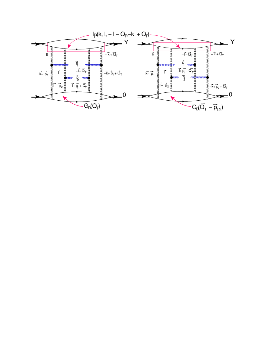
d2σdy1dy2d2pT1d2pT2(Fig.3a)1pT12pT22d2QTGD(QT)\displaystyle\frac{d^{2}\sigma}{dy_{1}\,dy_{2}d^{2}p_{T1}d^{2}p_{T2}}\left({Fig.~{}\ref{pdba}}-a\right)\,\,\propto\,\frac{1}{p^{2}_{T1}\,p^{2}_{T2}}\,\int d^{2}Q_{T}\,G_{D}\left(Q_{T}\right)
×\displaystyle\times d2kTd2lTIP(𝒌T,𝒍T,𝒍T,𝒌T)IP(𝒌T𝒑T1,𝒌T+𝒑T1)IP(𝒍T𝒑T2,𝒍T+𝒑T2)𝒌T2(𝒌𝒑1)T2𝒍T2(𝒍𝒑2)T2superscript𝑑2subscript𝑘𝑇superscript𝑑2subscript𝑙𝑇subscript𝐼𝑃subscript𝒌𝑇subscript𝒍𝑇subscript𝒍𝑇subscript𝒌𝑇subscript𝐼𝑃subscript𝒌𝑇subscript𝒑𝑇1subscript𝒌𝑇subscript𝒑𝑇1subscript𝐼𝑃subscript𝒍𝑇subscript𝒑𝑇2subscript𝒍𝑇subscript𝒑𝑇2subscriptsuperscript𝒌2𝑇subscriptsuperscript𝒌subscript𝒑12𝑇subscriptsuperscript𝒍2𝑇subscriptsuperscript𝒍subscript𝒑22𝑇\displaystyle\int d^{2}k_{T}\,d^{2}l_{T}\,I_{P}\left(\boldsymbol{k}_{T},\boldsymbol{l}_{T},-\boldsymbol{l}_{T},-\boldsymbol{k}_{T}\right)\frac{I_{P}\left(\boldsymbol{k}_{T}-\boldsymbol{p}_{T1},-\boldsymbol{k}_{T}+\boldsymbol{p}_{T1}\right)\,I_{P}\left(\boldsymbol{l}_{T}-\boldsymbol{p}_{T2},-\boldsymbol{l}_{T}+\boldsymbol{p}_{T2}\right)}{\boldsymbol{k}^{2}_{T}\,\left(\boldsymbol{k}-\boldsymbol{p}_{1}\right)^{2}_{T}\,\boldsymbol{l}^{2}_{T}\,\left(\boldsymbol{l}-\boldsymbol{p}_{2}\right)^{2}_{T}}
Refer to caption
Figure 3: The double inclusive production of two gluons with rapidities y1subscript𝑦1y_{1} and y2subscript𝑦2y_{2} and transverse momenta 𝒑T1subscript𝒑𝑇1\boldsymbol{p}_{T1} and 𝒑T2subscript𝒑𝑇2\boldsymbol{p}_{T2} in the Born Approximation of perturbative QCD. The interference diagram of Fig. 3-b yields the correlation function C(RN|𝒑T1𝒑T2|)𝐶subscript𝑅𝑁subscript𝒑𝑇1subscript𝒑𝑇2C\left(R_{N}|\boldsymbol{p}_{T1}\,-\,\boldsymbol{p}_{T2}|\right) of Eq. (2). The solid lines denote nucleons in the deuterons, which are illustated by double lines

Unfortunately, we cannot treat the impact factors IPsubscript𝐼𝑃I_{P} theoretically in the case of nucleon. The phenomenological approach to IPsubscript𝐼𝑃I_{P} has been discussed in Refs.LERE ; GLMBE , and we will return to this below. For the moment we replace the nucleon by the state of a heavy quark and antiquark (onium), to study the key features of the impact factors in the framework of perturbative QCD (see Fig. 4). Introducing, the form factor of the onium in the form

F(QT)=d2rei12𝑸T𝒓|Ψonium(r)|2𝐹subscript𝑄𝑇superscript𝑑2𝑟superscript𝑒𝑖12subscript𝑸𝑇𝒓superscriptsubscriptΨonium𝑟2F\left(Q_{T}\right)\,\,=\,\,\int d^{2}r\,e^{i\frac{1}{2}\boldsymbol{Q}_{T}\cdot\boldsymbol{r}}\,|\Psi_{\rm onium}\left(r\right)|^{2} (13)

we can express the impact factor in the form

IP(𝒌T,𝒌T+𝑸T)subscript𝐼𝑃subscript𝒌𝑇subscript𝒌𝑇subscript𝑸𝑇\displaystyle I_{P}\left(\boldsymbol{k}_{T},-\boldsymbol{k}_{T}+\boldsymbol{Q}_{T}\right) =\displaystyle= F(𝑸T)F(2𝒌T+𝑸T);𝐹subscript𝑸𝑇𝐹2subscript𝒌𝑇subscript𝑸𝑇\displaystyle F\left(\boldsymbol{Q}_{T}\right)\,-\,F\left(2\boldsymbol{k}_{T}+\boldsymbol{Q}_{T}\right); (14)
IP(𝒌T,𝒍T,𝒍T+𝑸T,𝒌T+𝑸T)subscript𝐼𝑃subscript𝒌𝑇subscript𝒍𝑇subscript𝒍𝑇subscript𝑸𝑇subscript𝒌𝑇subscript𝑸𝑇\displaystyle I_{P}\left(\boldsymbol{k}_{T},\boldsymbol{l}_{T},-\boldsymbol{l}_{T}+\boldsymbol{Q}_{T},-\boldsymbol{k}_{T}+\boldsymbol{Q}_{T}\right) =\displaystyle= 1+F(2𝑸T)+F(2(𝒌T+𝒍T))+F(2(𝒌T𝒍T𝑸T))1𝐹2subscript𝑸𝑇𝐹2subscript𝒌𝑇subscript𝒍𝑇𝐹2subscript𝒌𝑇subscript𝒍𝑇subscript𝑸𝑇\displaystyle 1\,+\,F\left(2\boldsymbol{Q}_{T}\right)\,+\,F\left(2(\boldsymbol{k}_{T}+\boldsymbol{l}_{T})\right)\,+\,F\left(2(\boldsymbol{k}_{T}-\boldsymbol{l}_{T}-\boldsymbol{Q}_{T})\right) (15)
\displaystyle- F(2𝒌T)F(2(𝒌T𝑸T))F(2𝒍T)F(2(𝒍T+𝑸T))𝐹2subscript𝒌𝑇𝐹2subscript𝒌𝑇subscript𝑸𝑇𝐹2subscript𝒍𝑇𝐹2subscript𝒍𝑇subscript𝑸𝑇\displaystyle F\left(2\boldsymbol{k}_{T}\right)\,-\,F\left(2(\boldsymbol{k}_{T}-\boldsymbol{Q}_{T})\right)\,-\,F\left(2\boldsymbol{l}_{T}\right)\,-\,F\left(2(\boldsymbol{l}_{T}+\boldsymbol{Q}_{T})\right)

In Eq. (II.2) the impact factors are equal to

IP(𝒌T,𝒌T)subscript𝐼𝑃subscript𝒌𝑇subscript𝒌𝑇\displaystyle I_{P}\left(\boldsymbol{k}_{T},-\boldsymbol{k}_{T}\right) =\displaystyle= 1F(2𝒌T);IP(𝒍T,𝒍T)= 1F(2𝒍T);1𝐹2subscript𝒌𝑇subscript𝐼𝑃subscript𝒍𝑇subscript𝒍𝑇1𝐹2subscript𝒍𝑇\displaystyle 1\,-\,F\left(2\boldsymbol{k}_{T}\right);~{}~{}~{}~{}~{}~{}I_{P}\left(\boldsymbol{l}_{T},-\boldsymbol{l}_{T}\right)\,=\,1\,-\,F\left(2\boldsymbol{l}_{T}\right); (16)
IP(𝒌T,𝒍T,𝒍T,𝒌T)subscript𝐼𝑃subscript𝒌𝑇subscript𝒍𝑇subscript𝒍𝑇subscript𝒌𝑇\displaystyle I_{P}\left(\boldsymbol{k}_{T},\boldsymbol{l}_{T},-\boldsymbol{l}_{T},-\boldsymbol{k}_{T}\right) =\displaystyle= 2+F(2(𝒌T+𝒍T))+F(2(𝒌T𝒍T))F(2𝒌T)F(2(𝒌T))F(2𝒍T)F(2(𝒍T));2𝐹2subscript𝒌𝑇subscript𝒍𝑇𝐹2subscript𝒌𝑇subscript𝒍𝑇𝐹2subscript𝒌𝑇𝐹2subscript𝒌𝑇𝐹2subscript𝒍𝑇𝐹2subscript𝒍𝑇\displaystyle 2\,+\,F\left(2(\boldsymbol{k}_{T}+\boldsymbol{l}_{T})\right)+F\left(2(\boldsymbol{k}_{T}-\boldsymbol{l}_{T})\right)-F\left(2\boldsymbol{k}_{T}\right)\,-\,F\left(2(\boldsymbol{k}_{T})\right)-F\left(2\boldsymbol{l}_{T}\right)-F\left(2(\boldsymbol{l}_{T})\right); (17)

The integration over kTsubscript𝑘𝑇k_{T} and lTsubscript𝑙𝑇l_{T} lead to typical values of kT1/RNsimilar-tosubscript𝑘𝑇1subscript𝑅𝑁k_{T}\sim 1/R_{N} and lT1/RNsimilar-tosubscript𝑙𝑇1subscript𝑅𝑁l_{T}\sim 1/R_{N}, and it does not generate azimuthal angle correlations. Indeed, this is clear from the following features of IPsubscript𝐼𝑃I_{P} from Eq. (17):

RNkT1,RNlT1;IP(𝒌T,𝒍T,𝒍T,𝒌T)formulae-sequencemuch-less-thansubscript𝑅𝑁subscript𝑘𝑇1much-less-thansubscript𝑅𝑁subscript𝑙𝑇1subscript𝐼𝑃subscript𝒌𝑇subscript𝒍𝑇subscript𝒍𝑇subscript𝒌𝑇\displaystyle R_{N}\,k_{T}\ll 1,R_{N}\,l_{T}\ll 1;~{}~{}~{}~{}I_{P}\left(\boldsymbol{k}_{T},\boldsymbol{l}_{T},-\boldsymbol{l}_{T},-\boldsymbol{k}_{T}\right)\, proportional-to\displaystyle\propto kT2lT2;subscriptsuperscript𝑘2𝑇subscriptsuperscript𝑙2𝑇\displaystyle\,k^{2}_{T}\,l^{2}_{T};
RNkT1,RNlT1;IP(𝒌T,𝒍T,𝒍T,𝒌T)formulae-sequencemuch-less-thansubscript𝑅𝑁subscript𝑘𝑇1much-greater-thansubscript𝑅𝑁subscript𝑙𝑇1subscript𝐼𝑃subscript𝒌𝑇subscript𝒍𝑇subscript𝒍𝑇subscript𝒌𝑇\displaystyle R_{N}\,k_{T}\ll 1,R_{N}\,l_{T}\gg 1;~{}~{}~{}~{}I_{P}\left(\boldsymbol{k}_{T},\boldsymbol{l}_{T},-\boldsymbol{l}_{T},-\boldsymbol{k}_{T}\right)\, proportional-to\displaystyle\propto kT2;subscriptsuperscript𝑘2𝑇\displaystyle\,k^{2}_{T};
RNkT1,RNlT1;IP(𝒌T,𝒍T,𝒍T,𝒌T)formulae-sequencemuch-greater-thansubscript𝑅𝑁subscript𝑘𝑇1much-less-thansubscript𝑅𝑁subscript𝑙𝑇1subscript𝐼𝑃subscript𝒌𝑇subscript𝒍𝑇subscript𝒍𝑇subscript𝒌𝑇\displaystyle R_{N}\,k_{T}\gg 1,R_{N}\,l_{T}\ll 1;~{}~{}~{}~{}I_{P}\left(\boldsymbol{k}_{T},\boldsymbol{l}_{T},-\boldsymbol{l}_{T},-\boldsymbol{k}_{T}\right)\, proportional-to\displaystyle\propto lT2;subscriptsuperscript𝑙2𝑇\displaystyle l^{2}_{T};
RNkT1,RNlT1;IP(𝒌T,𝒍T,𝒍T,𝒌T)formulae-sequencemuch-greater-thansubscript𝑅𝑁subscript𝑘𝑇1much-greater-thansubscript𝑅𝑁subscript𝑙𝑇1subscript𝐼𝑃subscript𝒌𝑇subscript𝒍𝑇subscript𝒍𝑇subscript𝒌𝑇\displaystyle R_{N}\,k_{T}\gg 1,R_{N}\,l_{T}\gg 1;~{}~{}~{}~{}I_{P}\left(\boldsymbol{k}_{T},\boldsymbol{l}_{T},-\boldsymbol{l}_{T},-\boldsymbol{k}_{T}\right)\, proportional-to\displaystyle\propto 1;1\displaystyle 1; (18)
Refer to caption
Figure 4: The impact factors for onium for RNkT>1subscript𝑅𝑁subscript𝑘𝑇1R_{N}k_{T}>1, RNlT>1subscript𝑅𝑁subscript𝑙𝑇1R_{N}l_{T}>1 and RNQT>1subscript𝑅𝑁subscript𝑄𝑇1R_{N}Q_{T}>1

In the diagram of Fig. 3-b one can see that GD(𝑸T𝒑12)subscript𝐺𝐷subscript𝑸𝑇subscript𝒑12G_{D}\left(\boldsymbol{Q}_{T}-\boldsymbol{p}_{12}\right) regulates that |𝑸T𝒑12|subscript𝑸𝑇subscript𝒑12|\boldsymbol{Q}_{T}-\boldsymbol{p}_{12}| is of the order of 1/RD1subscript𝑅𝐷1/R_{D}. This means that we can put 𝑸T=𝒑12subscript𝑸𝑇subscript𝒑12\boldsymbol{Q}_{T}=\boldsymbol{p}_{12} in all parts of diagrams, since the typical values of kTsubscript𝑘𝑇k_{T} and lTsubscript𝑙𝑇l_{T} are about 1/RN 1/RDmuch-greater-than1subscript𝑅𝑁1subscript𝑅𝐷1/R_{N}\,\gg\,1/R_{D}. Therefore, the diagram of Fig. 3-b can be reduced to the form

d2σdy1dy2d2pT1d2pT2(Fig.3b)1pT12pT22d2QTGD(𝑸T𝒑12)\displaystyle\frac{d^{2}\sigma}{dy_{1}\,dy_{2}d^{2}p_{T1}d^{2}p_{T2}}\left({Fig.~{}\ref{pdba}}-b\right)\,\,\propto\,\frac{1}{p^{2}_{T1}\,p^{2}_{T2}}\,\int d^{2}Q_{T}G_{D}\left(\boldsymbol{Q}_{T}-\boldsymbol{p}_{12}\right) (19)
×\displaystyle\times d2kTd2lTIP(𝒌T,𝒍T,𝒍T𝒑12,𝒌T+𝒑12)IP(𝒌T𝒑T1,𝒌T+𝒑T1)IP(𝒍T𝒑T2,𝒍T+𝒑T2)superscript𝑑2subscript𝑘𝑇superscript𝑑2subscript𝑙𝑇subscript𝐼𝑃subscript𝒌𝑇subscript𝒍𝑇subscript𝒍𝑇subscript𝒑12subscript𝒌𝑇subscript𝒑12subscript𝐼𝑃subscript𝒌𝑇subscript𝒑𝑇1subscript𝒌𝑇subscript𝒑𝑇1subscript𝐼𝑃subscript𝒍𝑇subscript𝒑𝑇2subscript𝒍𝑇subscript𝒑𝑇2\displaystyle\int d^{2}k_{T}\,d^{2}l_{T}\,I_{P}\left(\boldsymbol{k}_{T},\boldsymbol{l}_{T},-\boldsymbol{l}_{T}-\boldsymbol{p}_{12},-\boldsymbol{k}_{T}+\boldsymbol{p}_{12}\right)\,I_{P}\left(\boldsymbol{k}_{T}-\boldsymbol{p}_{T1},-\boldsymbol{k}_{T}+\boldsymbol{p}_{T1}\right)\,I_{P}\left(\boldsymbol{l}_{T}-\boldsymbol{p}_{T2},-\boldsymbol{l}_{T}+\boldsymbol{p}_{T2}\right)
×\displaystyle\times {(1(𝒌𝒑1)T2(𝒍+𝒑12)T2+1kT2(𝒍𝒑2)T2)(𝒍𝒌+𝒑12)T2pT,12kT2(𝒌𝒑1)T2(𝒍𝒑2)T2(𝒍+𝒑12)2}1subscriptsuperscript𝒌subscript𝒑12𝑇subscriptsuperscript𝒍subscript𝒑122𝑇1subscriptsuperscript𝑘2𝑇subscriptsuperscript𝒍subscript𝒑22𝑇subscriptsuperscript𝒍𝒌subscript𝒑122𝑇subscriptsuperscript𝑝2𝑇1subscriptsuperscript𝑘2𝑇subscriptsuperscript𝒌subscript𝒑12𝑇subscriptsuperscript𝒍subscript𝒑22𝑇superscript𝒍subscript𝒑122\displaystyle\Bigg{\{}\Bigg{(}\frac{1}{\left(\boldsymbol{k}-\boldsymbol{p}_{1}\right)^{2}_{T}\,\left(\boldsymbol{l}+\boldsymbol{p}_{12}\right)^{2}_{T}}\,+\,\frac{1}{k^{2}_{T}\,\left(\boldsymbol{l}-\boldsymbol{p}_{2}\right)^{2}_{T}}\Bigg{)}\,-\,\frac{\left(\boldsymbol{l}-\boldsymbol{k}+\boldsymbol{p}_{12}\right)^{2}_{T}\,p^{2}_{T,1}}{k^{2}_{T}\,\left(\boldsymbol{k}-\boldsymbol{p}_{1}\right)^{2}_{T}\,\left(\boldsymbol{l}-\boldsymbol{p}_{2}\right)^{2}_{T}\,\left(\boldsymbol{l}+\boldsymbol{p}_{12}\right)^{2}}\Bigg{\}}
×\displaystyle\times {(1(𝒍𝒑2)T2(𝒌𝒑12)T2+1lT2(𝒌𝒑1)T2)(𝒍𝒌+𝒑12)T2pT,22lT2(𝒍𝒑2)T2(𝒌𝒑1)T2(𝒌𝒑12)2}1subscriptsuperscript𝒍subscript𝒑22𝑇subscriptsuperscript𝒌subscript𝒑122𝑇1subscriptsuperscript𝑙2𝑇subscriptsuperscript𝒌subscript𝒑12𝑇subscriptsuperscript𝒍𝒌subscript𝒑122𝑇subscriptsuperscript𝑝2𝑇2subscriptsuperscript𝑙2𝑇subscriptsuperscript𝒍subscript𝒑22𝑇subscriptsuperscript𝒌subscript𝒑12𝑇superscript𝒌subscript𝒑122\displaystyle\Bigg{\{}\Bigg{(}\frac{1}{\left(\boldsymbol{l}-\boldsymbol{p}_{2}\right)^{2}_{T}\,\left(\boldsymbol{k}-\boldsymbol{p}_{12}\right)^{2}_{T}}\,+\,\frac{1}{l^{2}_{T}\,\left(\boldsymbol{k}-\boldsymbol{p}_{1}\right)^{2}_{T}}\Bigg{)}\,-\,\frac{\left(\boldsymbol{l}-\boldsymbol{k}+\boldsymbol{p}_{12}\right)^{2}_{T}\,p^{2}_{T,2}}{l^{2}_{T}\,\left(\boldsymbol{l}-\boldsymbol{p}_{2}\right)^{2}_{T}\,\left(\boldsymbol{k}-\boldsymbol{p}_{1}\right)^{2}_{T}\,\left(\boldsymbol{k}-\boldsymbol{p}_{12}\right)^{2}}\Bigg{\}}

The largest contributions to the integrals over kTsubscript𝑘𝑇k_{T} and lTsubscript𝑙𝑇l_{T} lead to the logarithmically large terms, which are proportional to ln(pT12RN2)ln(pT22RN2)subscriptsuperscript𝑝2𝑇1subscriptsuperscript𝑅2𝑁subscriptsuperscript𝑝2𝑇2subscriptsuperscript𝑅2𝑁\ln\left(p^{2}_{T1}\,R^{2}_{N}\right)\,\ln\left(p^{2}_{T2}\,R^{2}_{N}\right). These contribution stems from the terms which are proportional to 1/((𝒌𝒑1)T2)21superscriptsubscriptsuperscript𝒌subscript𝒑12𝑇21/\left(\left(\boldsymbol{k}-\boldsymbol{p}_{1}\right)^{2}_{T}\right)^{2}, and to 1/((𝒍𝒑2)T2)21superscriptsubscriptsuperscript𝒍subscript𝒑22𝑇21/\left(\left(\boldsymbol{l}-\boldsymbol{p}_{2}\right)^{2}_{T}\right)^{2}. We consider the kinematic region in the integration over kTsubscript𝑘𝑇k_{T} and lTsubscript𝑙𝑇l_{T}, where 𝒌T𝒑T1𝒌10subscript𝒌𝑇subscript𝒑𝑇1subscript𝒌10\boldsymbol{k}_{T}-\boldsymbol{p}_{T1}\equiv\boldsymbol{k}_{1}\to 0 and 𝒍T𝒑T2𝒍20subscript𝒍𝑇subscript𝒑𝑇2subscript𝒍20\boldsymbol{l}_{T}-\boldsymbol{p}_{T2}\equiv\boldsymbol{l}_{2}\to 0. For small k1pT2much-less-thansubscript𝑘1subscript𝑝𝑇2k_{1}\,\ll\,p_{T2} and l2pT1much-less-thansubscript𝑙2subscript𝑝𝑇1l_{2}\,\ll\,p_{T1} the product of curly brackets is equal to

1pT12{1k12+1l12(𝒌1𝒍2)2k12l22}1pT22{1k12+1l12(𝒌1𝒍2)2k12l22}=4(𝒌1𝒍2)2pT12pT22k14l24afterintegrationoverangle2pT12pT22k12l221subscriptsuperscript𝑝2𝑇11subscriptsuperscript𝑘211subscriptsuperscript𝑙21superscriptsubscript𝒌1subscript𝒍22subscriptsuperscript𝑘21subscriptsuperscript𝑙221subscriptsuperscript𝑝2𝑇21subscriptsuperscript𝑘211subscriptsuperscript𝑙21superscriptsubscript𝒌1subscript𝒍22subscriptsuperscript𝑘21subscriptsuperscript𝑙224superscriptsubscript𝒌1subscript𝒍22subscriptsuperscript𝑝2𝑇1subscriptsuperscript𝑝2𝑇2subscriptsuperscript𝑘41subscriptsuperscript𝑙42afterintegrationoverangle2subscriptsuperscriptp2T1subscriptsuperscriptp2T2subscriptsuperscriptk21subscriptsuperscriptl22\frac{1}{p^{2}_{T1}}\Bigg{\{}\frac{1}{k^{2}_{1}}\,+\,\frac{1}{l^{2}_{1}}\,-\,\frac{\left(\boldsymbol{k}_{1}\,-\,\boldsymbol{l}_{2}\right)^{2}}{k^{2}_{1}\,l^{2}_{2}}\Bigg{\}}\,\frac{1}{p^{2}_{T2}}\Bigg{\{}\frac{1}{k^{2}_{1}}\,+\,\frac{1}{l^{2}_{1}}\,-\,\frac{\left(\boldsymbol{k}_{1}\,-\,\boldsymbol{l}_{2}\right)^{2}}{k^{2}_{1}\,l^{2}_{2}}\Bigg{\}}=\,\frac{4\left(\boldsymbol{k}_{1}\cdot\boldsymbol{l}_{2}\right)^{2}}{p^{2}_{T1}\,p^{2}_{T2}\,k^{4}_{1}\,l^{4}_{2}}\,\xrightarrow{\rm after\,integration\,over\,angle}\,\frac{2}{p^{2}_{T1}\,p^{2}_{T2}\,k^{2}_{1}\,l^{2}_{2}} (20)

For RNk11much-less-thansubscript𝑅𝑁subscript𝑘11R_{N}k_{1}\ll 1 ,IP(𝒌T𝒑T1,𝒌T+𝒑T1)k12,I_{P}\left(\boldsymbol{k}_{T}-\boldsymbol{p}_{T1},-\boldsymbol{k}_{T}+\boldsymbol{p}_{T1}\right)\propto k^{2}_{1}, and the integral over k1subscript𝑘1k_{1} gives a small contribution of the order of 1/(RN2pT12)1subscriptsuperscript𝑅2𝑁subscriptsuperscript𝑝2𝑇11/(R^{2}_{N}p^{2}_{T1}). Recall that we can use the perturbative QCD approach only if RNpT1 1much-greater-thansubscript𝑅𝑁subscript𝑝𝑇11R_{N}p_{T1}\,\gg\,1 and RNpT2 1much-greater-thansubscript𝑅𝑁subscript𝑝𝑇21R_{N}p_{T2}\,\gg\,1. Therefore, the main contribution occurs from the region of integration (1/RN2)k1pT2much-less-than1subscriptsuperscript𝑅2𝑁subscript𝑘1much-less-thansubscript𝑝𝑇2(1/R^{2}_{N})\ll k_{1}\ll p_{T2} and (1/RN2)l1pT1much-less-than1subscriptsuperscript𝑅2𝑁subscript𝑙1much-less-thansubscript𝑝𝑇1(1/R^{2}_{N})\ll l_{1}\ll p_{T1}. Integration in this region leads to the contribution

d2σdy1dy2d2pT1d2pT2(Fig.3b)\displaystyle\frac{d^{2}\sigma}{dy_{1}\,dy_{2}d^{2}p_{T1}d^{2}p_{T2}}\left({Fig.~{}\ref{pdba}}-b\right)\,\, proportional-to\displaystyle\propto\, 1pT14pT24ln(pT12RN2)ln(pT22RN2)d2QTGD(𝑸T𝒑12)1subscriptsuperscript𝑝4𝑇1subscriptsuperscript𝑝4𝑇2subscriptsuperscript𝑝2𝑇1subscriptsuperscript𝑅2𝑁subscriptsuperscript𝑝2𝑇2subscriptsuperscript𝑅2𝑁superscript𝑑2subscript𝑄𝑇subscript𝐺𝐷subscript𝑸𝑇subscript𝒑12\displaystyle\frac{1}{p^{4}_{T1}\,p^{4}_{T2}}\,\ln\left(p^{2}_{T1}R^{2}_{N}\right)\ln\left(p^{2}_{T2}R^{2}_{N}\right)\int d^{2}Q_{T}G_{D}\left(\boldsymbol{Q}_{T}-\boldsymbol{p}_{12}\right) (21)
×\displaystyle\times IP(𝒑T1,𝒑T2,𝒑T1,𝒑T2)subscript𝐼𝑃subscript𝒑𝑇1subscript𝒑𝑇2subscript𝒑𝑇1subscript𝒑𝑇2\displaystyle I_{P}\left(\boldsymbol{p}_{T1},\boldsymbol{p}_{T2},-\boldsymbol{p}_{T1},-\boldsymbol{p}_{T2}\right)

Therefore, from this kinematic region the correlations are determined by the impact factor. Using the impact factor given in Eq. (15), we see that

IP(𝒑T1,𝒑T2,𝒑T1,𝒑T2)= 2+F(2(𝒑T1+𝒑T2))+F(2𝒑T,12)2F(2𝒑T1)2F(𝒑T2)subscript𝐼𝑃subscript𝒑𝑇1subscript𝒑𝑇2subscript𝒑𝑇1subscript𝒑𝑇22𝐹2subscript𝒑𝑇1subscript𝒑𝑇2𝐹2subscript𝒑𝑇122𝐹2subscript𝒑𝑇12𝐹subscript𝒑𝑇2I_{P}\left(\boldsymbol{p}_{T1},\boldsymbol{p}_{T2},\boldsymbol{p}_{T1},\boldsymbol{p}_{T2}\right)\,=\,2+F\left(2\left(\boldsymbol{p}_{T1}+\boldsymbol{p}_{T2}\right)\right)+F\left(2\boldsymbol{p}_{T,12}\right)-2F\left(2\boldsymbol{p}_{T1}\right)-2F\left(\boldsymbol{p}_{T2}\right) (22)

This function is symmetric with respect to ϕπϕitalic-ϕ𝜋italic-ϕ\phi\to\pi-\phi (𝒑T1𝒑T1subscript𝒑𝑇1subscript𝒑𝑇1\boldsymbol{p}_{T1}\to-\boldsymbol{p}_{T1}), and with such an impact factor, the Born approximation produces only vnsubscript𝑣𝑛v_{n} with even n𝑛n, as was noted in Ref.KOWE ; KOLUCOR . However, this conclusion is based on the impact factor of Eq. (15). Eq. (22) shows that this impact factor leads to pT,121/RNsimilar-tosubscript𝑝𝑇121subscript𝑅𝑁p_{T,12}\sim 1/R_{N}.

Refer to caption
Figure 5: The impact factors for onium for for RNkT>1subscript𝑅𝑁subscript𝑘𝑇1R_{N}k_{T}>1, RNlT>1subscript𝑅𝑁subscript𝑙𝑇1R_{N}l_{T}>1 and RNQT1subscript𝑅𝑁subscript𝑄𝑇1R_{N}Q_{T}\leq 1. The dashed lines denote the Coulomb gluons that form the onium bound state.

Note that the simple expression of Eq. (15) (see Fig. 4) is written for sufficiently hard gluons. For small values of QT=pT,12subscript𝑄𝑇subscript𝑝𝑇12Q_{T}=p_{T,12} we need to add the first diagram of Fig. 5, in which two gluons with large transverse momenta (about pT1subscript𝑝𝑇1p_{T1} or pT2subscript𝑝𝑇2p_{T2} ) but small QTsubscript𝑄𝑇Q_{T}. The final expression for the impact factor takes the form

IPF(𝒌T,𝒍T,𝒍T+𝑸T,𝒌T+𝑸T)=IP(𝒌T,𝒌T+𝑸T)IP(𝒍T,𝒍T𝑸T)+IP(𝒌T,𝒍T,𝒍T+𝑸T,𝒌T+𝑸T)Eq.(15)subscriptsuperscript𝐼𝐹𝑃subscript𝒌𝑇subscript𝒍𝑇subscript𝒍𝑇subscript𝑸𝑇subscript𝒌𝑇subscript𝑸𝑇subscript𝐼𝑃subscript𝒌𝑇subscript𝒌𝑇subscript𝑸𝑇subscript𝐼𝑃subscript𝒍𝑇subscript𝒍𝑇subscript𝑸𝑇subscriptsubscript𝐼𝑃subscript𝒌𝑇subscript𝒍𝑇subscript𝒍𝑇subscript𝑸𝑇subscript𝒌𝑇subscript𝑸𝑇formulae-sequenceEq15I^{F}_{P}\left(\boldsymbol{k}_{T},\boldsymbol{l}_{T},-\boldsymbol{l}_{T}+\boldsymbol{Q}_{T},-\boldsymbol{k}_{T}+\boldsymbol{Q}_{T}\right)\,=\,I_{P}\left(\boldsymbol{k}_{T},-\boldsymbol{k}_{T}+\boldsymbol{Q}_{T}\right)\,I_{P}\left(\boldsymbol{l}_{T},-\boldsymbol{l}_{T}-\boldsymbol{Q}_{T}\right)\,+\,\underbrace{I_{P}\left(\boldsymbol{k}_{T},\boldsymbol{l}_{T},-\boldsymbol{l}_{T}+\boldsymbol{Q}_{T},-\boldsymbol{k}_{T}+\boldsymbol{Q}_{T}\right)}_{\rm{Eq.~{}(\ref{IF2})}} (23)

The first term in Eq. (23) generates the correlation function which is proportional to F2(2𝒑T,12)superscript𝐹22subscript𝒑𝑇12F^{2}\left(2\boldsymbol{p}_{T,12}\right).

Summarizing, we see that the Born approximation of perturbative QCD, generates the correlation function which is determined by the impact factor of the nucleon, the typical correlation length is about RNsubscript𝑅𝑁R_{N}, and even for the unrealistic perturbative model of onium, this correlation function is not symmetric with respect to ϕπϕitalic-ϕ𝜋italic-ϕ\phi\to\pi-\phi. We will consider below the more realistic case, in leading log approximation of perturbative QCD. However, we would like to stress now, that the correlation function stems from the large non-perturbative distances of the order of the nucleon size.

II.3 Bose-Einstein correlation function with radius 𝑹𝑵proportional-toabsentsubscript𝑹𝑵\propto\,\,R_{N}: nucleon-nucleon interaction

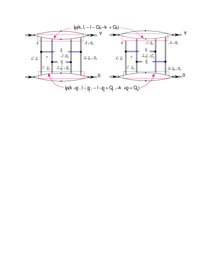
The correlations with Rc=RNsubscript𝑅𝑐subscript𝑅𝑁R_{c}=R_{N} are typical for the nucleon-nucleon interaction ( see Fig. 6 for the Born approximation of perturbative QCD). However, we will consider them below for the general case of the production of two parton showers, since we prefer to use a more phenomenological and realistic approach for the impact factors IPsubscript𝐼𝑃I_{P}, than we explored above, replacing the nucleon by the onium state.
Refer to caption
Figure 6: The double inclusive production of two gluons with rapidities y1subscript𝑦1y_{1} and y2subscript𝑦2y_{2} and transverse momenta 𝒑T1subscript𝒑𝑇1\boldsymbol{p}_{T1} and 𝒑T2subscript𝒑𝑇2\boldsymbol{p}_{T2} in the Born Approximation of perturbative QCD for the nucleon-nucleon interaction. The interference diagram of Fig. 6-b yields the correlation function C(RD|𝒑T1𝒑T2|)𝐶subscript𝑅𝐷subscript𝒑𝑇1subscript𝒑𝑇2C\left(R_{D}|\boldsymbol{p}_{T1}\,-\,\boldsymbol{p}_{T2}|\right) of Eq. (2). The solid lines denote nucleons in the deuterons, which are illustrated by double lines.

III Production of two parton showers

III.1 𝑹𝒄𝑹𝑫proportional-tosubscript𝑹𝒄subscript𝑹𝑫R_{c}\,\,\propto\,\,R_{D}

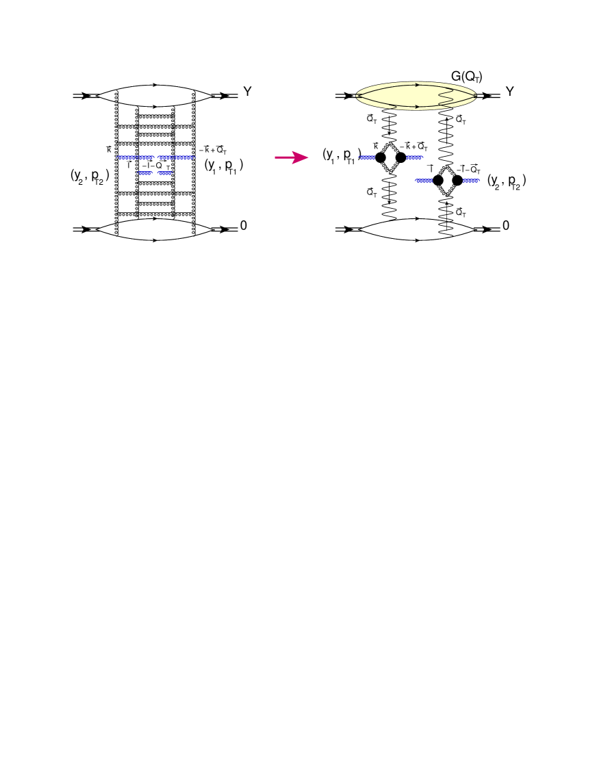
In this section we consider the general case of the production of two parton showers shown in Fig. 1. In the leading log approximation (LLA) of perturbative QCD, the structure of one parton shower is described by the BFKL PomeronBFKL ; LI .
Refer to caption
Figure 7: The double inclusive production of two gluons with rapidities y1subscript𝑦1y_{1} and y2subscript𝑦2y_{2} and transverse momenta 𝒑T1subscript𝒑𝑇1\boldsymbol{p}_{T1} and 𝒑T2subscript𝒑𝑇2\boldsymbol{p}_{T2}, for the exchange of two BFKL Pomerons which are denoted by wavy lines. This diagram is the LLA generalization of Fig. 2-a. The solid lines denote nucleons in the deuterons, which are indicated by double lines.

In the leading log approximation of perturbative QCD the Born diagram of Fig. 2-a can be generalized to Fig. 7. The contribution of this diagram can be written as follows

d2σdy1dy2d2pT1d2pT2(Fig.7)=(2πα¯SCF)21pT,12pT22d2QTGD2(QT)\displaystyle\frac{d^{2}\sigma}{dy_{1}\,dy_{2}d^{2}p_{T1}d^{2}p_{T2}}\left({Fig.~{}\ref{ddspom}}\right)\,\,=\,\,\left(\frac{2\pi\bar{\alpha}_{S}}{C_{F}}\right)^{2}\frac{1}{p^{2}_{T,1}\,p^{2}_{T2}}\int d^{2}Q_{T}G^{2}_{D}\left(Q_{T}\right) (24)
×\displaystyle\times (d2kTϕGN(Yy1;𝒌T,𝒌T+𝑸T)ϕGN(y1;𝒌T𝒑T1,𝒌T+𝒑T1+𝑸T))superscript𝑑2subscript𝑘𝑇subscriptsuperscriptitalic-ϕ𝑁𝐺𝑌subscript𝑦1subscript𝒌𝑇subscript𝒌𝑇subscript𝑸𝑇subscriptsuperscriptitalic-ϕ𝑁𝐺subscript𝑦1subscript𝒌𝑇subscript𝒑𝑇1subscript𝒌𝑇subscript𝒑𝑇1subscript𝑸𝑇\displaystyle\,\Bigg{(}\int d^{2}k_{T}\,\,\phi^{N}_{G}\left(Y-y_{1};\boldsymbol{k}_{T},-\boldsymbol{k}_{T}+\boldsymbol{Q}_{T}\right)\,\phi^{N}_{G}\left(y_{1};\boldsymbol{k}_{T}-\boldsymbol{p}_{T1},-\boldsymbol{k}_{T}+\boldsymbol{p}_{T1}+\boldsymbol{Q}_{T}\right)\Bigg{)}
×\displaystyle\times (d2lTϕGN(Yy2;𝒍T,𝒍T𝑸T)ϕGN(y2;𝒍T𝒑T2,𝒍T+𝒑T2𝑸T))superscript𝑑2subscript𝑙𝑇subscriptsuperscriptitalic-ϕ𝑁𝐺𝑌subscript𝑦2subscript𝒍𝑇subscript𝒍𝑇subscript𝑸𝑇subscriptsuperscriptitalic-ϕ𝑁𝐺subscript𝑦2subscript𝒍𝑇subscript𝒑𝑇2subscript𝒍𝑇subscript𝒑𝑇2subscript𝑸𝑇\displaystyle\,\Bigg{(}\int d^{2}l_{T}\,\,\phi^{N}_{G}\left(Y-y_{2};\boldsymbol{l}_{T},-\boldsymbol{l}_{T}-\boldsymbol{Q}_{T}\right)\,\phi^{N}_{G}\left(y_{2};\boldsymbol{l}_{T}-\boldsymbol{p}_{T2},-\boldsymbol{l}_{T}+\boldsymbol{p}_{T2}-\boldsymbol{Q}_{T}\right)\Bigg{)}

where ϕGN(y,𝒌T,𝒌T+𝑸T)subscriptsuperscriptitalic-ϕ𝑁𝐺𝑦subscript𝒌𝑇subscript𝒌𝑇subscript𝑸𝑇\phi^{N}_{G}\left(y,\boldsymbol{k}_{T},-\boldsymbol{k}_{T}+\boldsymbol{Q}_{T}\right) denotes the probability to find a gluon with rapidity y𝑦y and transverse momentum ksubscript𝑘perpendicular-tok_{\perp}, in the process with momentum transferred QTsubscript𝑄𝑇Q_{T}. In Eq. (24) α¯S=αSNc/πsubscript¯𝛼𝑆subscript𝛼𝑆subscript𝑁𝑐𝜋\bar{\alpha}_{S}\,=\,\alpha_{S}N_{c}/\pi with the number of colours equal to Ncsubscript𝑁𝑐N_{c}. ϕGNsubscriptsuperscriptitalic-ϕ𝑁𝐺\phi^{N}_{G} are the solutions of the BFKL evolution equation

ϕGN(y,𝒌T,𝒌T+𝑸T)ysubscriptsuperscriptitalic-ϕ𝑁𝐺𝑦subscript𝒌𝑇subscript𝒌𝑇subscript𝑸𝑇𝑦\displaystyle\frac{\partial\phi^{N}_{G}\left(y,\boldsymbol{k}_{T},-\boldsymbol{k}_{T}+\boldsymbol{Q}_{T}\right)}{\partial y}\, =\displaystyle= α¯Sd2kT2πK(QT;kT,kT)ϕGN(y,𝒌T,𝒌T+𝑸T)subscript¯𝛼𝑆superscript𝑑2subscriptsuperscript𝑘𝑇2𝜋𝐾subscript𝑄𝑇subscript𝑘𝑇subscriptsuperscript𝑘𝑇subscriptsuperscriptitalic-ϕ𝑁𝐺𝑦subscriptsuperscript𝒌bold-′𝑇subscriptsuperscript𝒌bold-′𝑇subscript𝑸𝑇\displaystyle\,\bar{\alpha}_{S}\int\frac{d^{2}k^{\prime}_{T}}{2\pi}\,K\left(Q_{T};k_{T},k^{\prime}_{T}\right)\,\phi^{N}_{G}\left(y,\boldsymbol{k^{\prime}}_{T},-\boldsymbol{k^{\prime}}_{T}+\boldsymbol{Q}_{T}\right)\,\,
\displaystyle- (ωG(𝑸T𝒌T)+ωG(𝒌T))ϕGN(y,𝒌T,𝒌T+𝑸T)subscript𝜔𝐺subscript𝑸𝑇subscript𝒌𝑇subscript𝜔𝐺subscript𝒌𝑇subscriptsuperscriptitalic-ϕ𝑁𝐺𝑦subscript𝒌𝑇subscript𝒌𝑇subscript𝑸𝑇\displaystyle\,\,\left(\omega_{G}\left(\boldsymbol{Q}_{T}-\boldsymbol{k}_{T}\right)\,+\,\omega_{G}\left(\boldsymbol{k}_{T}\right)\right)\phi^{N}_{G}\left(y,\boldsymbol{k}_{T},-\boldsymbol{k}_{T}+\boldsymbol{Q}_{T}\right)

where

K(QT,kT,kT)𝐾subscript𝑄𝑇subscript𝑘𝑇subscriptsuperscript𝑘𝑇\displaystyle K\left(Q_{T},k_{T},k^{\prime}_{T}\right)\, =\displaystyle= 1(𝒌T𝒌T)2{kT2kT2+(𝑸T𝒌T)2(𝑸T𝒌T)2(𝒌T𝒌T)2kT2(𝑸T𝒌T)2}1superscriptsubscript𝒌𝑇subscriptsuperscript𝒌bold-′𝑇2subscriptsuperscript𝑘2𝑇subscriptsuperscript𝑘2𝑇superscriptsubscript𝑸𝑇subscript𝒌𝑇2superscriptsubscript𝑸𝑇subscriptsuperscript𝒌bold-′𝑇2superscriptsubscript𝒌𝑇subscriptsuperscript𝒌bold-′𝑇2subscriptsuperscript𝑘2𝑇superscriptsubscript𝑸𝑇subscriptsuperscript𝒌bold-′𝑇2\displaystyle\,\frac{1}{\left(\boldsymbol{k}_{T}-\boldsymbol{k^{\prime}}_{T}\right)^{2}}\Bigg{\{}\frac{k^{2}_{T}}{k^{\prime 2}_{T}}\,+\,\frac{\left(\boldsymbol{Q}_{T}-\boldsymbol{k}_{T}\right)^{2}}{\left(\boldsymbol{Q}_{T}-\boldsymbol{k^{\prime}}_{T}\right)^{2}}\,\,-\,\,\frac{\left(\boldsymbol{k}_{T}-\boldsymbol{k^{\prime}}_{T}\right)^{2}}{k^{\prime 2}_{T}\,\left(\boldsymbol{Q}_{T}-\boldsymbol{k^{\prime}}_{T}\right)^{2}}\Bigg{\}} (26)
ωG(𝒌T)subscript𝜔𝐺subscript𝒌𝑇\displaystyle\omega_{G}\left(\boldsymbol{k}_{T}\right) =\displaystyle= 12α¯SkT2d2kT2π1kT2(𝒌T𝒌T)212subscript¯𝛼𝑆subscriptsuperscript𝑘2𝑇superscript𝑑2subscriptsuperscript𝑘𝑇2𝜋1subscriptsuperscript𝑘2𝑇superscriptsubscript𝒌𝑇subscriptsuperscript𝒌bold-′𝑇2\displaystyle\frac{1}{2}\bar{\alpha}_{S}k^{2}_{T}\int\frac{d^{2}k^{\prime}_{T}}{2\pi}\frac{1}{k^{\prime 2}_{T}\,\left(\boldsymbol{k}_{T}-\boldsymbol{k^{\prime}}_{T}\right)^{2}}

The typical momenta in ϕGNsubscriptsuperscriptitalic-ϕ𝑁𝐺\phi^{N}_{G} is about 1/RN1subscript𝑅𝑁1/R_{N} or larger, (about pT1subscript𝑝𝑇1p_{T1}(pT2subscript𝑝𝑇2p_{T2}) or Qssubscript𝑄𝑠Q_{s}, where Qssubscript𝑄𝑠Q_{s} denotes the saturation scale. Bearing this in mind, and noting that QT1/RD 1/RNsimilar-tosubscript𝑄𝑇1subscript𝑅𝐷much-less-than1subscript𝑅𝑁Q_{T}\sim 1/R_{D}\,\ll\,1/R_{N} we can put QT=0subscript𝑄𝑇0Q_{T}=0, in the arguments of ϕGNsubscriptsuperscriptitalic-ϕ𝑁𝐺\phi^{N}_{G}. This simplifies Eq. (24) reducing it to the following expression

d2σdy1dy2d2pT1d2pT2(Fig.7)=d2σdy1d2pT1d2σdy2d2pT2×d2QTGD2(QT)\frac{d^{2}\sigma}{dy_{1}\,dy_{2}d^{2}p_{T1}d^{2}p_{T2}}\left({Fig.~{}\ref{ddspom}}\right)\,\,=\,\,\frac{d^{2}\sigma}{dy_{1}\ d^{2}p_{T1}}\,\frac{d^{2}\sigma}{dy_{2}\ d^{2}p_{T2}}\,\times\,\int d^{2}Q_{T}G^{2}_{D}\left(Q_{T}\right) (27)

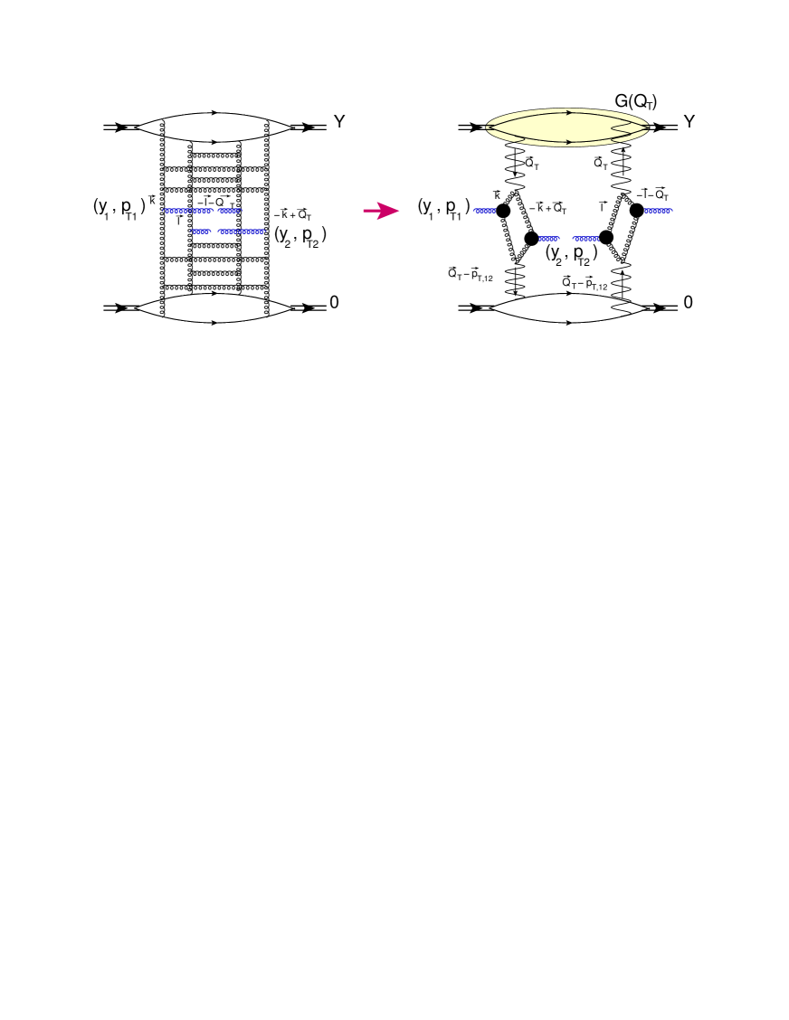
The diagram of Fig. 2-b in the LLA, simplifies the expression for the exchange of two BFKL Pomerons, but with more complicated vertices. Using Eq. (II.1) and considering α¯S(y1y2)1subscript¯𝛼𝑆subscript𝑦1subscript𝑦21\bar{\alpha}_{S}\left(y_{1}-y_{2}\right)\leq 1, we can write this exchange in the form that is represented in Fig. 8, and its contribution has the following form
Refer to caption
Figure 8: The double inclusive production of two gluons with rapidities y1subscript𝑦1y_{1} and y2subscript𝑦2y_{2} and transverse momenta 𝒑T1subscript𝒑𝑇1\boldsymbol{p}_{T1} and 𝒑T2subscript𝒑𝑇2\boldsymbol{p}_{T2} for the exchange of two BFKL Pomerons which are denoted by wavy lines. This diagram is the LLA generalization of Fig. 2-b. The solid lines denote nucleons in the deuterons, which are represented by double lines.
d2σdy1dy2d2pT1d2pT2(Fig.8)=12(2πα¯SCF)2d2QTGD(QT)GD(𝑸T𝒑T,12)\displaystyle\frac{d^{2}\sigma}{dy_{1}\,dy_{2}d^{2}p_{T1}d^{2}p_{T2}}\left({Fig.~{}\ref{ddipom}}\right)\,\,=\,\,\frac{1}{2}\left(\frac{2\pi\bar{\alpha}_{S}}{C_{F}}\right)^{2}\int d^{2}Q_{T}G_{D}\left(Q_{T}\right)\,G_{D}\left(\boldsymbol{Q}_{T}-\boldsymbol{p}_{T,12}\right)
×\displaystyle\times (d2kTϕGN(Yy1;𝒌T,𝒌T+𝑸T)Γμ(kT,pT1)Γμ(𝒌T+𝑸T,pT2)ϕGN(y2;𝒌T𝒑T1,𝒌T+𝒑T2+𝑸T))superscript𝑑2subscript𝑘𝑇subscriptsuperscriptitalic-ϕ𝑁𝐺𝑌subscript𝑦1subscript𝒌𝑇subscript𝒌𝑇subscript𝑸𝑇subscriptΓ𝜇subscript𝑘𝑇subscript𝑝𝑇1subscriptΓ𝜇subscript𝒌𝑇subscript𝑸𝑇subscript𝑝𝑇2subscriptsuperscriptitalic-ϕ𝑁𝐺subscript𝑦2subscript𝒌𝑇subscript𝒑𝑇1subscript𝒌𝑇subscript𝒑𝑇2subscript𝑸𝑇\displaystyle\,\Bigg{(}\int d^{2}k_{T}\,\,\phi^{N}_{G}\left(Y-y_{1};\boldsymbol{k}_{T},-\boldsymbol{k}_{T}+\boldsymbol{Q}_{T}\right)\,\Gamma_{\mu}\left(k_{T},p_{T1}\right)\,\Gamma_{\mu}\left(-\boldsymbol{k}_{T}+\boldsymbol{Q}_{T},p_{T2}\right)\,\phi^{N}_{G}\left(y_{2};\boldsymbol{k}_{T}-\boldsymbol{p}_{T1},-\boldsymbol{k}_{T}+\boldsymbol{p}_{T2}+\boldsymbol{Q}_{T}\right)\Bigg{)}
×\displaystyle\times (d2lTϕGN(Yy1;𝒍T,𝒍T𝑸T)Γμ(lT,pT1)Γμ(𝒍T𝑸T,pT2)ϕGN(y2;𝒍T𝒑T2,𝒍T+𝒑T1𝑸T))superscript𝑑2subscript𝑙𝑇subscriptsuperscriptitalic-ϕ𝑁𝐺𝑌subscript𝑦1subscript𝒍𝑇subscript𝒍𝑇subscript𝑸𝑇subscriptΓ𝜇subscript𝑙𝑇subscript𝑝𝑇1subscriptΓ𝜇subscript𝒍𝑇subscript𝑸𝑇subscript𝑝𝑇2subscriptsuperscriptitalic-ϕ𝑁𝐺subscript𝑦2subscript𝒍𝑇subscript𝒑𝑇2subscript𝒍𝑇subscript𝒑𝑇1subscript𝑸𝑇\displaystyle\,\Bigg{(}\int d^{2}l_{T}\,\,\phi^{N}_{G}\left(Y-y_{1};\boldsymbol{l}_{T},-\boldsymbol{l}_{T}-\boldsymbol{Q}_{T}\right)\,\Gamma_{\mu}\left(l_{T},p_{T1}\right)\,\Gamma_{\mu}\left(-\boldsymbol{l}_{T}-\boldsymbol{Q}_{T},p_{T2}\right)\phi^{N}_{G}\left(y_{2};\boldsymbol{l}_{T}-\boldsymbol{p}_{T2},-\boldsymbol{l}_{T}+\boldsymbol{p}_{T1}-\boldsymbol{Q}_{T}\right)\Bigg{)}

Since QT1/RB 1/RNsimilar-tosubscript𝑄𝑇1subscript𝑅𝐵much-less-than1subscript𝑅𝑁Q_{T}\sim 1/R_{B}\,\ll\,1/R_{N} as well as |𝑸T𝒑T,12|1/RD 1/RNsimilar-tosubscript𝑸𝑇subscript𝒑𝑇121subscript𝑅𝐷much-less-than1subscript𝑅𝑁|\boldsymbol{Q}_{T}-\boldsymbol{p}_{T,12}|\sim 1/R_{D}\,\ll\,1/R_{N}, we can take both QT=0subscript𝑄𝑇0Q_{T}=0 and pT,12=0subscript𝑝𝑇120p_{T,12}=0, but it is not sufficient to reduce Eq. (III.1) to Eq. (12). In addition we need to assume that α¯S(y1y2) 1subscript¯𝛼𝑆subscript𝑦1subscript𝑦21\bar{\alpha}_{S}\left(y_{1}-y_{2}\right)\,\leq\,1. Making this assumption we can replace y2subscript𝑦2y_{2} in ϕGN(y2;𝒌T𝒑T1,𝒌T+𝒑T2+𝑸T)subscriptsuperscriptitalic-ϕ𝑁𝐺subscript𝑦2subscript𝒌𝑇subscript𝒑𝑇1subscript𝒌𝑇subscript𝒑𝑇2subscript𝑸𝑇\phi^{N}_{G}\left(y_{2};\boldsymbol{k}_{T}-\boldsymbol{p}_{T1},-\boldsymbol{k}_{T}+\boldsymbol{p}_{T2}+\boldsymbol{Q}_{T}\right) by y1subscript𝑦1y_{1} and Yy1𝑌subscript𝑦1Y-y_{1}, in ϕGN(Yy1;𝒍T,𝒍T𝑸T)subscriptsuperscriptitalic-ϕ𝑁𝐺𝑌subscript𝑦1subscript𝒍𝑇subscript𝒍𝑇subscript𝑸𝑇\phi^{N}_{G}\left(Y-y_{1};\boldsymbol{l}_{T},-\boldsymbol{l}_{T}-\boldsymbol{Q}_{T}\right) by Yy2𝑌subscript𝑦2Y-y_{2}. After these changes Eq. (III.1) can be reduced to the following expression

d2σdy1dy2d2pT1d2pT2(Fig.8)=d2σdy1d2pT1d2σdy2d2pT2×d2QTGD(QT)GD(𝑸T+𝒑T,12)\frac{d^{2}\sigma}{dy_{1}\,dy_{2}d^{2}p_{T1}d^{2}p_{T2}}\left({Fig.~{}\ref{ddipom}}\right)\,\,=\,\,\frac{d^{2}\sigma}{dy_{1}\ d^{2}p_{T1}}\,\frac{d^{2}\sigma}{dy_{2}\ d^{2}p_{T2}}\,\times\,\int d^{2}Q_{T}G_{D}\left(Q_{T}\right)\,G_{D}\left(\boldsymbol{Q}_{T}+\boldsymbol{p}_{T,12}\right) (29)

Eq. (27) and Eq. (29) lead to the same correlation function (C(RDpT,12)𝐶subscript𝑅𝐷subscript𝑝𝑇12C\left(R_{D}\,p_{T,12}\right)) Eq. (12) as in the Born approximation.

III.2 𝑹𝒄𝑹𝑵proportional-tosubscript𝑹𝒄subscript𝑹𝑵R_{c}\,\,\propto\,\,R_{N}

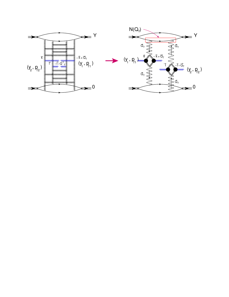
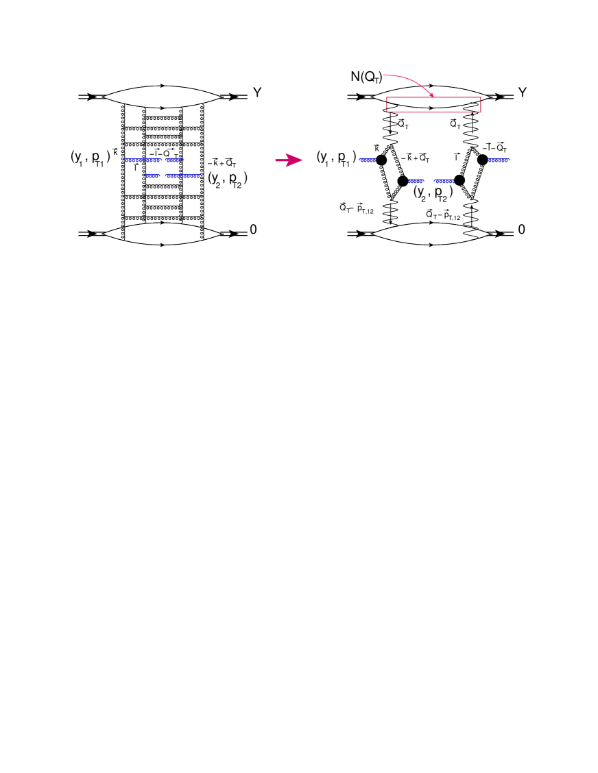
In LLA the diagrams of the Born approximation of Fig. 3 can be generalized in the same way as has been discussed above. Fig. 3-a takes the form of Fig. 9 while the interference diagram of Fig. 3-b becomes Fig. 10.
Refer to caption
Figure 9: The Mueller diagramMUDI for the double inclusive production of two gluons with rapidities y1subscript𝑦1y_{1} and y2subscript𝑦2y_{2} and transverse momenta 𝒑T1subscript𝒑𝑇1\boldsymbol{p}_{T1} and 𝒑T2subscript𝒑𝑇2\boldsymbol{p}_{T2}, for the exchange of two BFKL Pomerons which are denoted by wavy lines. This diagram is the LLA generalization of Fig. 3-a. The solid lines denote nucleons in the deuterons, which are illustrated by double lines.

The contribution of the diagram of Fig. 9 can be written as follows

d2σdy1dy2d2pT1d2pT2(Fig.9)=(2πα¯SCF)21pT,12pT22d2QTN(QT)GD2(QT)\displaystyle\frac{d^{2}\sigma}{dy_{1}\,dy_{2}d^{2}p_{T1}d^{2}p_{T2}}\left({Fig.~{}\ref{pdspom}}\right)\,\,=\,\,\left(\frac{2\pi\bar{\alpha}_{S}}{C_{F}}\right)^{2}\frac{1}{p^{2}_{T,1}\,p^{2}_{T2}}\int d^{2}Q_{T}\,N\left(Q_{T}\right)\,G^{2}_{D}\left(Q_{T}\right) (30)
×\displaystyle\times (d2kTϕGN(Yy1;𝒌T,𝒌T+𝑸T)ϕGN(y1;𝒌T𝒑T1,𝒌T+𝒑T1+𝑸T))superscript𝑑2subscript𝑘𝑇subscriptsuperscriptitalic-ϕ𝑁𝐺𝑌subscript𝑦1subscript𝒌𝑇subscript𝒌𝑇subscript𝑸𝑇subscriptsuperscriptitalic-ϕ𝑁𝐺subscript𝑦1subscript𝒌𝑇subscript𝒑𝑇1subscript𝒌𝑇subscript𝒑𝑇1subscript𝑸𝑇\displaystyle\,\Bigg{(}\int d^{2}k_{T}\,\,\phi^{N}_{G}\left(Y-y_{1};\boldsymbol{k}_{T},-\boldsymbol{k}_{T}+\boldsymbol{Q}_{T}\right)\,\phi^{N}_{G}\left(y_{1};\boldsymbol{k}_{T}-\boldsymbol{p}_{T1},-\boldsymbol{k}_{T}+\boldsymbol{p}_{T1}+\boldsymbol{Q}_{T}\right)\Bigg{)}
×\displaystyle\times (d2lTϕGN(Yy2;𝒍T,𝒍T𝑸T)ϕGN(y2;𝒍T𝒑T2,𝒍T+𝒑T2𝑸T))superscript𝑑2subscript𝑙𝑇subscriptsuperscriptitalic-ϕ𝑁𝐺𝑌subscript𝑦2subscript𝒍𝑇subscript𝒍𝑇subscript𝑸𝑇subscriptsuperscriptitalic-ϕ𝑁𝐺subscript𝑦2subscript𝒍𝑇subscript𝒑𝑇2subscript𝒍𝑇subscript𝒑𝑇2subscript𝑸𝑇\displaystyle\,\Bigg{(}\int d^{2}l_{T}\,\,\phi^{N}_{G}\left(Y-y_{2};\boldsymbol{l}_{T},-\boldsymbol{l}_{T}-\boldsymbol{Q}_{T}\right)\,\phi^{N}_{G}\left(y_{2};\boldsymbol{l}_{T}-\boldsymbol{p}_{T2},-\boldsymbol{l}_{T}+\boldsymbol{p}_{T2}-\boldsymbol{Q}_{T}\right)\Bigg{)}

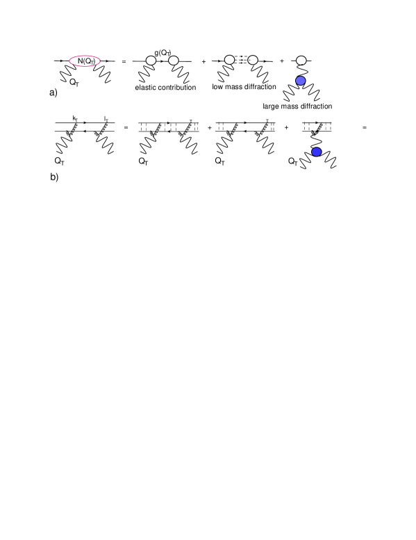
where N(QT)𝑁subscript𝑄𝑇N\left(Q_{T}\right) denotes the integral over all energies of the imaginary part of the Pomeron-nucleon scattering amplitude. This amplitude was introduced in Gribov’s Pomeron calculusGRIBPOM , but it has been proven that we can use this formalism in LLA of perturbative QCDGLR . N(QT)𝑁subscript𝑄𝑇N\left(Q_{T}\right) has the following general form(see Fig. 11)

N(QT)=g2(QT)elasticscattering+Mi=mM0g2(QT;Mi)diffractioninlowmasses+M0dM2M2ϕGN(yM,QT=0;{})G3IP(QT,{})diffractioninhighmassesN\left(Q_{T}\right)\,\,=\,\,\underbrace{g^{2}\left(Q_{T}\right)}_{\rm elastic\,scattering}\,+\,\underbrace{\sum^{M_{0}}_{M_{i}=m}g^{2}\left(Q_{T};M_{i}\right)}_{\rm diffraction\,in\,low\,masses}\,+\,\underbrace{\int_{M_{0}}\frac{dM^{2}}{M^{2}}\phi^{N}_{G}\left(y_{M},Q_{T}=0;\{\dots\}\right)\,G_{3{I\!\!P}}\left(Q_{T},\{\dots\}\right)}_{diffraction\,in\,high\,masses} (31)

where G3IPsubscript𝐺3𝐼𝑃G_{3{I\!\!P}} is the triple BFKL Pomeron vertex, and {}\{\dots\} denotes all transverse momenta which we need to integrate over. yM=ln(M2/M02)subscript𝑦𝑀superscript𝑀2subscriptsuperscript𝑀20y_{M}=\ln\left(M^{2}/M^{2}_{0}\right).

Fig. 11-b shows how all contributions correspond to the onium case, where we can use perturbative QCD for theoretical estimates.
Refer to caption
Figure 10: The Mueller diagram for the double inclusive production of two gluons with rapidities y1subscript𝑦1y_{1} and y2subscript𝑦2y_{2} and transverse momenta 𝒑T1subscript𝒑𝑇1\boldsymbol{p}_{T1} and 𝒑T2subscript𝒑𝑇2\boldsymbol{p}_{T2}, for the exchange of two BFKL Pomerons which are denoted by wavy lines. This diagram is the LLA generalization of Fig. 3-b. The solid lines denote nucleons in the deuterons, which are illustated by double lines.

Since QT1/RD 1.RNformulae-sequencesimilar-tosubscript𝑄𝑇1subscript𝑅𝐷much-less-than1subscript𝑅𝑁Q_{T}\sim 1/R_{D}\,\ll\,1.R_{N}, and all other transverse momenta in Fig. 9 are either of the order of 1/RN1subscript𝑅𝑁1/R_{N} or larger ( of the order of pT1subscript𝑝𝑇1p_{T1},pT2subscript𝑝𝑇2p_{T2} or Qssubscript𝑄𝑠Q_{s}, where Qssubscript𝑄𝑠Q_{s} is the saturation scale), we can safely put QT=0subscript𝑄𝑇0Q_{T}=0 and reduce this contribution to the factorized form:

d2σdy1dy2d2pT1d2pT2(Fig.9)=d2σdy1d2pT1d2σdy2d2pT2N(QT=0)d2QTGD(QT)\frac{d^{2}\sigma}{dy_{1}\,dy_{2}d^{2}p_{T1}d^{2}p_{T2}}\left({Fig.~{}\ref{pdspom}}\right)\,\,=\frac{d^{2}\sigma}{dy_{1}\,d^{2}p_{T1}}\,\frac{d^{2}\sigma}{dy_{2}\,d^{2}p_{T2}}\,N\left(Q_{T}=0\right)\,\int d^{2}Q_{T}G_{D}\left(Q_{T}\right) (32)

The contribution of the relevant diagram, which is shown in Fig. 10, can be written in the form:

d2σdy1dy2d2pT1d2pT2(Fig.10)=12(2πα¯SCF)2d2QTN(QT)GD(𝑸T𝒑T,12)\displaystyle\frac{d^{2}\sigma}{dy_{1}\,dy_{2}d^{2}p_{T1}d^{2}p_{T2}}\left({Fig.~{}\ref{pdipom}}\right)\,\,=\,\,\frac{1}{2}\left(\frac{2\pi\bar{\alpha}_{S}}{C_{F}}\right)^{2}\int d^{2}Q_{T}N\left(Q_{T}\right)\,G_{D}\left(\boldsymbol{Q}_{T}-\boldsymbol{p}_{T,12}\right) (33)
×\displaystyle\times (d2kTϕGN(Yy1;𝒌T,𝒌T+𝑸T)Γμ(kT,pT1)Γμ(𝒌T+𝑸T,pT2)ϕGN(y2;𝒌T𝒑T1,𝒌T+𝒑T2+𝑸T))superscript𝑑2subscript𝑘𝑇subscriptsuperscriptitalic-ϕ𝑁𝐺𝑌subscript𝑦1subscript𝒌𝑇subscript𝒌𝑇subscript𝑸𝑇subscriptΓ𝜇subscript𝑘𝑇subscript𝑝𝑇1subscriptΓ𝜇subscript𝒌𝑇subscript𝑸𝑇subscript𝑝𝑇2subscriptsuperscriptitalic-ϕ𝑁𝐺subscript𝑦2subscript𝒌𝑇subscript𝒑𝑇1subscript𝒌𝑇subscript𝒑𝑇2subscript𝑸𝑇\displaystyle\,\Bigg{(}\int d^{2}k_{T}\,\,\phi^{N}_{G}\left(Y-y_{1};\boldsymbol{k}_{T},-\boldsymbol{k}_{T}+\boldsymbol{Q}_{T}\right)\,\Gamma_{\mu}\left(k_{T},p_{T1}\right)\,\Gamma_{\mu}\left(-\boldsymbol{k}_{T}+\boldsymbol{Q}_{T},p_{T2}\right)\,\phi^{N}_{G}\left(y_{2};\boldsymbol{k}_{T}-\boldsymbol{p}_{T1},-\boldsymbol{k}_{T}+\boldsymbol{p}_{T2}+\boldsymbol{Q}_{T}\right)\Bigg{)}
×\displaystyle\times (d2lTϕGN(Yy1;𝒍T,𝒍T𝑸T)Γμ(lT,pT1)Γμ(𝒍T𝑸T,pT2)ϕGN(y2;𝒍T𝒑T2,𝒍T+𝒑T1𝑸T))superscript𝑑2subscript𝑙𝑇subscriptsuperscriptitalic-ϕ𝑁𝐺𝑌subscript𝑦1subscript𝒍𝑇subscript𝒍𝑇subscript𝑸𝑇subscriptΓ𝜇subscript𝑙𝑇subscript𝑝𝑇1subscriptΓ𝜇subscript𝒍𝑇subscript𝑸𝑇subscript𝑝𝑇2subscriptsuperscriptitalic-ϕ𝑁𝐺subscript𝑦2subscript𝒍𝑇subscript𝒑𝑇2subscript𝒍𝑇subscript𝒑𝑇1subscript𝑸𝑇\displaystyle\,\Bigg{(}\int d^{2}l_{T}\,\,\phi^{N}_{G}\left(Y-y_{1};\boldsymbol{l}_{T},-\boldsymbol{l}_{T}-\boldsymbol{Q}_{T}\right)\,\Gamma_{\mu}\left(l_{T},p_{T1}\right)\,\Gamma_{\mu}\left(-\boldsymbol{l}_{T}-\boldsymbol{Q}_{T},p_{T2}\right)\phi^{N}_{G}\left(y_{2};\boldsymbol{l}_{T}-\boldsymbol{p}_{T2},-\boldsymbol{l}_{T}+\boldsymbol{p}_{T1}-\boldsymbol{Q}_{T}\right)\Bigg{)}

Integration over QTsubscript𝑄𝑇Q_{T} leads to 𝑸T𝒑T,121/RD  1/RNsimilar-tosubscript𝑸𝑇subscript𝒑𝑇121subscript𝑅𝐷much-less-than1subscript𝑅𝑁\boldsymbol{Q}_{T}-\boldsymbol{p}_{T,12}\sim 1/R_{D}\,\ll\,\,1/R_{N} and, therefore, as in the Born approximation we can put 𝑸T=𝒑T,12subscript𝑸𝑇subscript𝒑𝑇12\boldsymbol{Q}_{T}=\boldsymbol{p}_{T,12}. In Eq. (33) we have two sources of pT,12subscript𝑝𝑇12p_{T,12} behavior: N(pT,12)𝑁subscript𝑝𝑇12N\left(p_{T,12}\right) and ϕGNsubscriptsuperscriptitalic-ϕ𝑁𝐺\phi^{N}_{G}. Replacing 𝑸T=𝒑T,12subscript𝑸𝑇subscript𝒑𝑇12\boldsymbol{Q}_{T}=\boldsymbol{p}_{T,12} we obtain

d2σdy1dy2d2pT1d2pT2(Fig.10)=12(2πα¯SCF)2d2QTN(pT,12)GD(𝑸T𝒑T,12)\displaystyle\frac{d^{2}\sigma}{dy_{1}\,dy_{2}d^{2}p_{T1}d^{2}p_{T2}}\left({Fig.~{}\ref{pdipom}}\right)\,\,=\,\,\frac{1}{2}\left(\frac{2\pi\bar{\alpha}_{S}}{C_{F}}\right)^{2}\int d^{2}Q_{T}N\left(p_{T,12}\right)\,G_{D}\left(\boldsymbol{Q}_{T}-\boldsymbol{p}_{T,12}\right) (34)
×\displaystyle\times (d2kTϕGN(Yy1;𝒌T,𝒌T+𝒑T,12)1kT2(𝒌T𝒑T,12)2(𝒌T𝒑T,1)4ϕGN(y2;𝒌T𝒑T1,𝒌T+𝒑T1)\displaystyle\,\Bigg{(}\int d^{2}k_{T}\,\,\phi^{N}_{G}\left(Y-y_{1};\boldsymbol{k}_{T},-\boldsymbol{k}_{T}+\boldsymbol{p}_{T,12}\right)\,\frac{1}{k^{2}_{T}\,\left(\boldsymbol{k}_{T}-\boldsymbol{p}_{T,12}\right)^{2}\left(\boldsymbol{k}_{T}-\boldsymbol{p}_{T,1}\right)^{4}}\phi^{N}_{G}\left(y_{2};\boldsymbol{k}_{T}-\boldsymbol{p}_{T1},-\boldsymbol{k}_{T}+\boldsymbol{p}_{T1}\right)
×\displaystyle\times {(𝒌T𝒑T,12)2(𝒌T𝒑T,1)2pT22+kT2(𝒌T𝒑T,1𝒑T,12)2pT21pT,122pT,122kT2(𝒌T𝒑T,12)2pT21pT,22})\displaystyle\Bigg{\{}\frac{\left(\boldsymbol{k}_{T}-\boldsymbol{p}_{T,12}\right)^{2}\,\left(\boldsymbol{k}_{T}-\boldsymbol{p}_{T,1}\right)^{2}}{p^{2}_{T2}}\,+\,\frac{k^{2}_{T}\,\left(\boldsymbol{k}_{T}-\boldsymbol{p}_{T,1}-\boldsymbol{p}_{T,12}\right)^{2}}{p^{1}_{T2}}\,-\,p^{2}_{T,12}\,-\,p^{2}_{T,12}\frac{k^{2}_{T}\,\left(\boldsymbol{k}_{T}-\boldsymbol{p}_{T,12}\right)^{2}}{p^{1}_{T2}p^{2}_{T,2}}\Bigg{\}}\Bigg{)}
×\displaystyle\times (d2lTϕGN(Yy1;𝒍T,𝒍T𝒑T,12)1lT2(𝒍T+𝒑T,12)2(𝒍T𝒑T,2)4ϕGN(y2;𝒍T𝒑T2,𝒍T+𝒑T2)\displaystyle\,\Bigg{(}\int d^{2}l_{T}\,\,\phi^{N}_{G}\left(Y-y_{1};\boldsymbol{l}_{T},-\boldsymbol{l}_{T}-\boldsymbol{p}_{T,12}\right)\,\,\frac{1}{l^{2}_{T}\,\left(\boldsymbol{l}_{T}+\boldsymbol{p}_{T,12}\right)^{2}\left(\boldsymbol{l}_{T}-\boldsymbol{p}_{T,2}\right)^{4}}\phi^{N}_{G}\left(y_{2};\boldsymbol{l}_{T}-\boldsymbol{p}_{T2},-\boldsymbol{l}_{T}+\boldsymbol{p}_{T2}\right)
×\displaystyle\times {(𝒍T+𝒑T,12)2(𝒍T𝒑T,1)2pT22+lT2(𝒍T𝒑T,2)2pT21pT,122pT,122lT2(𝒍T+𝒑T,12)2pT21pT,22})\displaystyle\Bigg{\{}\frac{\left(\boldsymbol{l}_{T}+\boldsymbol{p}_{T,12}\right)^{2}\,\left(\boldsymbol{l}_{T}-\boldsymbol{p}_{T,1}\right)^{2}}{p^{2}_{T2}}\,+\,\frac{l^{2}_{T}\,\left(\boldsymbol{l}_{T}-\boldsymbol{p}_{T,2}\right)^{2}}{p^{1}_{T2}}\,-\,p^{2}_{T,12}\,-\,p^{2}_{T,12}\frac{l^{2}_{T}\,\left(\boldsymbol{l}_{T}+\boldsymbol{p}_{T,12}\right)^{2}}{p^{1}_{T2}p^{2}_{T,2}}\Bigg{\}}\Bigg{)}

The products of GμGμsubscript𝐺𝜇subscript𝐺𝜇G_{\mu}G_{\mu} are written in Eq. (34) {}\{\dots\} explicitly using Eq. (6), and ϕDNsubscriptsuperscriptitalic-ϕ𝑁𝐷\phi^{N}_{D} are the solution of Eq. (III.1). Recall that ϕDN(𝒌T,𝒌T+𝑸T)subscriptsuperscriptitalic-ϕ𝑁𝐷subscript𝒌𝑇subscript𝒌𝑇subscript𝑸𝑇\phi^{N}_{D}\left(\boldsymbol{k}_{T},-\boldsymbol{k}_{T}+\boldsymbol{Q}_{T}\right) vanishes both at kT0subscript𝑘𝑇0k_{T}\to 0 and 𝒌T𝑸T0subscript𝒌𝑇subscript𝑸𝑇0\boldsymbol{k}_{T}-\boldsymbol{Q}_{T}\to 0. Since the products of Gμsubscript𝐺𝜇G_{\mu} vanish at 𝒌T𝒑T1 0subscript𝒌𝑇subscript𝒑𝑇1 0\boldsymbol{k}_{T}-\boldsymbol{p}_{T1}\,\to\,0 or 𝒍T𝒑T2 0subscript𝒍𝑇subscript𝒑𝑇2 0\boldsymbol{l}_{T}-\boldsymbol{p}_{T2}\,\to\,0, respectively, we can conclude that the integrals over kTsubscript𝑘𝑇k_{T} and lTsubscript𝑙𝑇l_{T} do not have large contributions at kTsubscript𝑘𝑇k_{T} of the order of pT1subscript𝑝𝑇1p_{T1}, and at lTsubscript𝑙𝑇l_{T} of the order of pT2subscript𝑝𝑇2p_{T2}.

Refer to caption
Figure 11: The structure of the amplitude N(QT)𝑁subscript𝑄𝑇N\left(Q_{T}\right): Fig. 11-a for the BFKL Pomeron-nucleon interaction and Fig. 11-b for the BFKL Pomeron-onium interactions. The blob shows the triple BFKL Pomeron vertex which is the same for both figures. The dashed vertical lines describe the Coulomb gluons that create the bound state: onium.

In the appendix we show that the typical value of QTsubscript𝑄𝑇Q_{T} for the BFKL Pomeron ϕGN(Y;kT,kT,QT)subscriptsuperscriptitalic-ϕ𝑁𝐺𝑌subscriptsuperscript𝑘𝑇subscript𝑘𝑇subscript𝑄𝑇\phi^{N}_{G}\left(Y;k^{\prime}_{T},k_{T},Q_{T}\right) is determined by the smallest value of transverse momentum QTmin{k;T,kT}Q_{T}\sim min\{k;_{T},k_{T}\}. In our case this means that QT=pT,121/RNpT1subscript𝑄𝑇subscript𝑝𝑇12similar-to1subscript𝑅𝑁much-greater-thansubscript𝑝𝑇1Q_{T}=p_{T,12}\,\sim 1/R_{N}\,\gg\,p_{T1} and/or pT2subscript𝑝𝑇2p_{T2}.

Therefore, we can re-write Eq. (34) as follows:

d2σdy1dy2d2pT1d2pT2(Fig.10)\displaystyle\frac{d^{2}\sigma}{dy_{1}\,dy_{2}d^{2}p_{T1}d^{2}p_{T2}}\left({Fig.~{}\ref{pdipom}}\right)\, =\displaystyle= 12(2πα¯SCF)21pT12pT22d2QTN(pT,12)GD(𝑸T𝒑T,12)12superscript2𝜋subscript¯𝛼𝑆subscript𝐶𝐹21subscriptsuperscript𝑝2𝑇1subscriptsuperscript𝑝2𝑇2superscript𝑑2subscript𝑄𝑇𝑁subscript𝑝𝑇12subscript𝐺𝐷subscript𝑸𝑇subscript𝒑𝑇12\displaystyle\,\,\frac{1}{2}\left(\frac{2\pi\bar{\alpha}_{S}}{C_{F}}\right)^{2}\frac{1}{p^{2}_{T1}\,p^{2}_{T2}}\,\int d^{2}Q_{T}N\left(p_{T,12}\right)\,G_{D}\left(\boldsymbol{Q}_{T}-\boldsymbol{p}_{T,12}\right) (35)
×\displaystyle\times (d2kTϕGN(Yy1;𝒌T,𝒌T)ϕGN(y2;𝒌T𝒑T1,𝒌T+𝒑T1))superscript𝑑2subscript𝑘𝑇subscriptsuperscriptitalic-ϕ𝑁𝐺𝑌subscript𝑦1subscript𝒌𝑇subscript𝒌𝑇subscriptsuperscriptitalic-ϕ𝑁𝐺subscript𝑦2subscript𝒌𝑇subscript𝒑𝑇1subscript𝒌𝑇subscript𝒑𝑇1\displaystyle\,\Bigg{(}\int d^{2}k_{T}\,\,\phi^{N}_{G}\left(Y-y_{1};\boldsymbol{k}_{T},-\boldsymbol{k}_{T}\right)\,\phi^{N}_{G}\left(y_{2};\boldsymbol{k}_{T}-\boldsymbol{p}_{T1},-\boldsymbol{k}_{T}+\boldsymbol{p}_{T1}\right)\Bigg{)}
×\displaystyle\times (d2lTϕGN(Yy1;𝒍T,𝒍T)ϕGN(y2;𝒍T𝒑T2,𝒍T+𝒑T2))superscript𝑑2subscript𝑙𝑇subscriptsuperscriptitalic-ϕ𝑁𝐺𝑌subscript𝑦1subscript𝒍𝑇subscript𝒍𝑇subscriptsuperscriptitalic-ϕ𝑁𝐺subscript𝑦2subscript𝒍𝑇subscript𝒑𝑇2subscript𝒍𝑇subscript𝒑𝑇2\displaystyle\Bigg{(}\int d^{2}l_{T}\,\,\phi^{N}_{G}\left(Y-y_{1};\boldsymbol{l}_{T},-\boldsymbol{l}_{T}\right)\,\phi^{N}_{G}\left(y_{2};\boldsymbol{l}_{T}-\boldsymbol{p}_{T2},-\boldsymbol{l}_{T}+\boldsymbol{p}_{T2}\right)\Bigg{)}

In Eq. (35) we introduce ϕGN(𝒌t,𝒌T)=(1/kT2)ϕGN(𝒌t,𝒌T)(Eq.(34))\phi^{N}_{G}\left(\boldsymbol{k}_{t},-\boldsymbol{k}_{T}\right)=(1/k^{2}_{T})\phi^{N}_{G}\left(\boldsymbol{k}_{t},-\boldsymbol{k}_{T}\right)({Eq.~{}(\ref{RN4})}). Comparing Eq. (32) and Eq. (35), one can see that the correlation function is equal to

C(RN2pT,122)=N(p122)𝐶subscriptsuperscript𝑅2𝑁subscriptsuperscript𝑝2𝑇12𝑁subscriptsuperscript𝑝212C\left(R^{2}_{N}\,p^{2}_{T,12}\right)\,\,=\,\,N\left(p^{2}_{12}\right) (36)

for α¯S(y1y2)1subscript¯𝛼𝑆subscript𝑦1subscript𝑦21\bar{\alpha}_{S}(y_{1}-y_{2})\leq 1.

The three terms of N(QT)𝑁subscript𝑄𝑇N\left(Q_{T}\right) are shown in Fig. 11-a. The first contribution N(QT)=g2(QT)𝑁subscript𝑄𝑇superscript𝑔2subscript𝑄𝑇N\left(Q_{T}\right)\,=\,g^{2}\left(Q_{T}\right), can easily be evaluated from the differential elastic cross section, which is proportional to g4(QT)superscript𝑔4subscript𝑄𝑇g^{4}\left(Q_{T}\right). Recall, that the BFKL Pomeron does not generate the shrinkage of the diffraction peak seen in the experimental data. This indicates that the exchange of the single BFKL Pomeron is not sufficient to describe the high energy amplitude, and we need to use a more phenomenological approach to describe the elastic contribution to the correlation function (see Ref.GLMBE in which we tried to describe these correlations using a particular model for high energy scattering, which is based on CGC/saturation approach).

For the onium, g(QT)𝑔subscript𝑄𝑇g\left(Q_{T}\right) can be calculated (see Fig. 11-b and Eq. (76)) in the following way

g(QT)=Vonium(𝑸T)𝑔subscript𝑄𝑇superscript𝑉oniumsubscript𝑸𝑇\displaystyle g\left(Q_{T}\right)\,=\,V^{\rm onium}\left(\boldsymbol{Q}_{T}\right)\, =\displaystyle= d2kTIP(𝒌T,𝒌T+𝑸T)Vpr(𝒌T,𝑸T)superscript𝑑2subscriptsuperscript𝑘𝑇subscript𝐼𝑃subscript𝒌𝑇subscriptsuperscript𝒌bold-′𝑇subscript𝑸𝑇superscript𝑉prsubscriptsuperscript𝒌bold-′𝑇subscript𝑸𝑇\displaystyle\,\int d^{2}k^{\prime}_{T}I_{P}\left(\boldsymbol{k}_{T},-\boldsymbol{k^{\prime}}_{T}+\boldsymbol{Q}_{T}\right)V^{\rm pr}\left(\boldsymbol{k^{\prime}}_{T},\boldsymbol{Q}_{T}\right)\, (37)
=\displaystyle= d2kT(F(QT)F(2𝒌T𝑸T))V12pr(𝒌𝑻,𝑸T)superscript𝑑2subscriptsuperscript𝑘𝑇𝐹subscript𝑄𝑇𝐹2subscriptsuperscript𝒌bold-′𝑇subscript𝑸𝑇subscriptsuperscript𝑉pr12subscriptsuperscript𝒌bold-′𝑻subscript𝑸𝑇\displaystyle\,\int d^{2}k^{\prime}_{T}\left(F\left(Q_{T}\right)-F\left(2\boldsymbol{k^{\prime}}_{T}-\boldsymbol{Q}_{T}\right)\right)\,V^{\rm pr}_{\frac{1}{2}}\left(\boldsymbol{k^{\prime}_{T}},\boldsymbol{Q}_{T}\right)

where Vprsuperscript𝑉prV^{\rm pr} is determined by Eq. (75). In Eq. (37) kT1/RNkTsimilar-tosubscriptsuperscript𝑘𝑇1subscript𝑅𝑁much-less-thansubscript𝑘𝑇k^{\prime}_{T}\sim 1/R_{N}\,\ll\,k_{T}. Assuming that F(QT)𝐹subscript𝑄𝑇F\left(Q_{T}\right) of Eq. (14) is equal to 1/(1+RN2QT2)11subscriptsuperscript𝑅2𝑁subscriptsuperscript𝑄2𝑇1/\left(1+R^{2}_{N}\,Q^{2}_{T}\right), we find that at large QTsubscript𝑄𝑇Q_{T}, g(RNQT)𝑔subscript𝑅𝑁subscript𝑄𝑇g\left(R_{N}\,Q_{T}\right) decreases as 1/QT1subscript𝑄𝑇1/Q_{T}.

The second term of Fig. 11-b can be evaluated from the process of diffraction dissociation in the region of small masses. However, we need to use a model for this term to be able to extract its QTsubscript𝑄𝑇Q_{T} dependence from the experimental data. For example, we can replace the sum of possible produced diffractive states by one state, as has been done in Ref.GLMBE . For the onium state this term has the following form

Ndiff(QT)=d2kTd2lTIP(𝒌T,𝒍T,𝒍T+𝑸T,𝒌T+𝑸T)Vpr(𝒌T;𝑸T)Vpr(𝒍T;𝑸T)subscript𝑁diffsubscript𝑄𝑇superscript𝑑2subscriptsuperscript𝑘𝑇superscript𝑑2subscriptsuperscript𝑙𝑇subscript𝐼𝑃subscript𝒌𝑇subscript𝒍𝑇subscript𝒍𝑇subscript𝑸𝑇subscript𝒌𝑇subscript𝑸𝑇superscript𝑉prsubscriptsuperscript𝒌bold-′𝑇subscript𝑸𝑇superscript𝑉prsubscriptsuperscript𝒍bold-′𝑇subscript𝑸𝑇N_{\rm diff}\left(Q_{T}\right)\,=\,\int d^{2}k^{\prime}_{T}\int d^{2}l^{\prime}_{T}\,I_{P}\left(\boldsymbol{k}_{T},\boldsymbol{l}_{T},-\boldsymbol{l}_{T}+\boldsymbol{Q}_{T},-\boldsymbol{k}_{T}+\boldsymbol{Q}_{T}\right)\,V^{\rm pr}\left(\boldsymbol{k^{\prime}}_{T};\boldsymbol{Q}_{T}\right)\,\,V^{\rm pr}\left(\boldsymbol{l^{\prime}}_{T};\boldsymbol{Q}_{T}\right) (38)

where IPsubscript𝐼𝑃I_{P} is taken from Eq. (15).

Using Eq. (75) we calculate Ndiff(QT)subscript𝑁diffsubscript𝑄𝑇N_{\rm diff}\left(Q_{T}\right) which decreases as 1/QT21subscriptsuperscript𝑄2𝑇1/Q^{2}_{T} at large QTsubscript𝑄𝑇Q_{T}.

III.3 𝑹𝒄  1/𝑸𝒔proportional-tosubscript𝑹𝒄1subscript𝑸𝒔R_{c}\,\,\propto\,\,1/Q_{s}

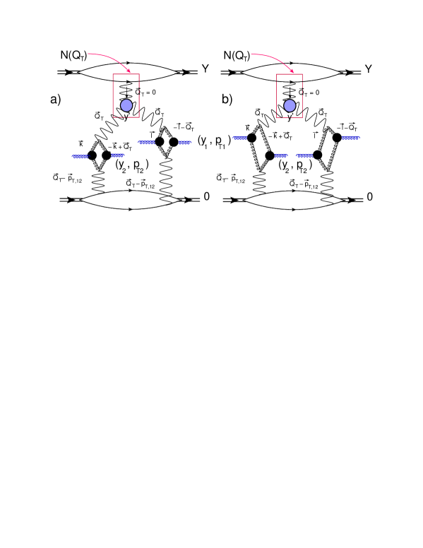
The last term in Fig. 11-a, gives the contribution of large mass production in the diffraction dissociation process. The QTsubscript𝑄𝑇Q_{T} dependence of this term, is determined by the triple BFKL Pomeron vertex in perturbative QCD (see Fig. 12). Therefore, this term generates correlations, whose length is determined by the BFKL Pomeron structure, and it is closely related to the typical saturation momentum Qssubscript𝑄𝑠Q_{s}.

Refer to caption
Figure 12: The large mass diffraction contribution to N(QT)𝑁subscript𝑄𝑇N\left(Q_{T}\right): the source for the correlation length of about 1/Qs1subscript𝑄𝑠1/Q_{s}. The blue blob denotes the triple BFKL Pomeron vertex. The red square indicates the contribution of N(QT)𝑁subscript𝑄𝑇N\left(Q_{T}\right), which includes the integration over rapidity ysuperscript𝑦y^{\prime}.

Comparing Fig. 12 with Fig. 9 and Fig. 10, one can see that the difference is only in expression for N(QT)𝑁subscript𝑄𝑇N\left(Q_{T}\right) which has the following form

Nlargemassdiffraction(QT)=dyϕGN(Yy;QT=0;qT,qT)d2qTG3IP(qT;kT,lT,QT)N_{\rm large\,mass\,diffraction}\left(Q_{T}\right)\,\,=\,\,\int\,d\,y^{\prime}\,\phi^{N}_{G}\left(Y-y^{\prime};Q_{T}=0;q_{T},q^{\prime}_{T}\right)d^{2}q^{\prime}_{T}G_{3{I\!\!P}}\left(q^{\prime}_{T};k^{\prime}_{T},l^{\prime}_{T},Q_{T}\right) (39)

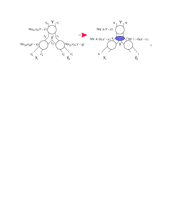
We can obtain the form of G3IPsubscript𝐺3𝐼𝑃G_{3{I\!\!P}} in momentum space starting from the coordinate representation, where the contribution of the triple Pomeron diagram of Fig. 13 is knownBRAUN ; KLP :

α¯Sd2x0d2x1d2x2x012x022x212N(x01,x01;𝒃𝒃;Yy)N(x02,x02;𝒃12𝒙21;yy1)N(x21,x21;𝒃12𝒙02;yy2)subscript¯𝛼𝑆superscript𝑑2subscript𝑥0superscript𝑑2subscript𝑥1superscript𝑑2subscript𝑥2subscriptsuperscript𝑥201subscriptsuperscript𝑥202subscriptsuperscript𝑥221𝑁subscriptsuperscript𝑥01subscript𝑥01𝒃superscript𝒃bold-′𝑌superscript𝑦𝑁subscriptsuperscript𝑥02subscript𝑥02superscript𝒃bold-′12subscript𝒙21superscript𝑦subscript𝑦1𝑁subscriptsuperscript𝑥21subscript𝑥21superscript𝒃bold-′12subscript𝒙02superscript𝑦subscript𝑦2\bar{\alpha}_{S}\int\frac{d^{2}x_{0}\,d^{2}x_{1}\,d^{2}x_{2}}{x^{2}_{01}\,x^{2}_{02}\,x^{2}_{21}}N\left(x^{\prime}_{01},x_{01};\boldsymbol{b}-\boldsymbol{b^{\prime}};Y-y^{\prime}\right)\,N\left(x^{\prime}_{02},x_{02};\boldsymbol{b^{\prime}}-\frac{1}{2}\boldsymbol{x}_{21};y^{\prime}-y_{1}\right)\,N\left(x^{\prime}_{21},x_{21};\boldsymbol{b^{\prime}}-\frac{1}{2}\boldsymbol{x}_{02};y^{\prime}-y_{2}\right) (40)

IntroducingKOLEB

N(x01,b;Y)=x012d2kd2QTei𝒌T𝒙01+i𝑸T𝒃N(kT,QT)𝑁subscript𝑥01𝑏𝑌subscriptsuperscript𝑥201superscript𝑑2𝑘superscript𝑑2subscript𝑄𝑇superscript𝑒𝑖subscript𝒌𝑇subscript𝒙01𝑖subscript𝑸𝑇𝒃𝑁subscript𝑘𝑇subscript𝑄𝑇N\left(x_{01},b;Y\right)\,\,=\,\,x^{2}_{01}\int d^{2}kd^{2}Q_{T}\,e^{i\boldsymbol{k}_{T}\cdot\boldsymbol{x}_{01}\,+\,i\,\boldsymbol{Q}_{T}\cdot\boldsymbol{b}}N\left(k_{T},Q_{T}\right) (41)

we see that Eq. (40) can be re-written in the form

α¯Sd2qTN(qT,qT,QT=0,Yy)G3IP(qT;kT,lT,QT)N(kT,kT,QT,yy1)N(lT,lT,QT,yy2)\bar{\alpha}_{S}\int d^{2}q^{\prime}_{T}\,N\left(q_{T},q^{\prime}_{T},Q_{T}=0,Y-y^{\prime}\right)\,G_{3{I\!\!P}}\left(q^{\prime}_{T};k^{\prime}_{T},l^{\prime}_{T},Q_{T}\right)N\left(k^{\prime}_{T},k_{T},Q_{T},y^{\prime}-y_{1}\right)\,N\left(l^{\prime}_{T},l_{T},-Q_{T},y^{\prime}-y_{2}\right) (42)

with

G3IP(qT;kT,lT,QT)=δ(2)(𝒌T𝒒+12𝑸T)δ(2)(𝒍T𝒒12𝑸T)subscript𝐺3𝐼𝑃subscriptsuperscript𝑞𝑇subscriptsuperscript𝑘𝑇subscriptsuperscript𝑙𝑇subscript𝑄𝑇superscript𝛿2subscriptsuperscript𝒌bold-′𝑇superscript𝒒bold-′12subscript𝑸𝑇superscript𝛿2subscriptsuperscript𝒍bold-′𝑇superscript𝒒bold-′12subscript𝑸𝑇G_{3{I\!\!P}}\left(q^{\prime}_{T};k^{\prime}_{T},l^{\prime}_{T},Q_{T}\right)\,\,=\,\,\delta^{(2)}\left(\boldsymbol{k^{\prime}}_{T}\,-\boldsymbol{q^{\prime}}\,+\frac{1}{2}\boldsymbol{Q}_{T}\right)\,\delta^{(2)}\left(\boldsymbol{l^{\prime}}_{T}\,-\boldsymbol{q^{\prime}}\,-\frac{1}{2}\boldsymbol{Q}_{T}\right)\, (43)
Refer to caption
Figure 13: The triple BFKL Pomeron vertex in coordinate and momentum representations. The blue blob denotes the triple Pomeron vertex

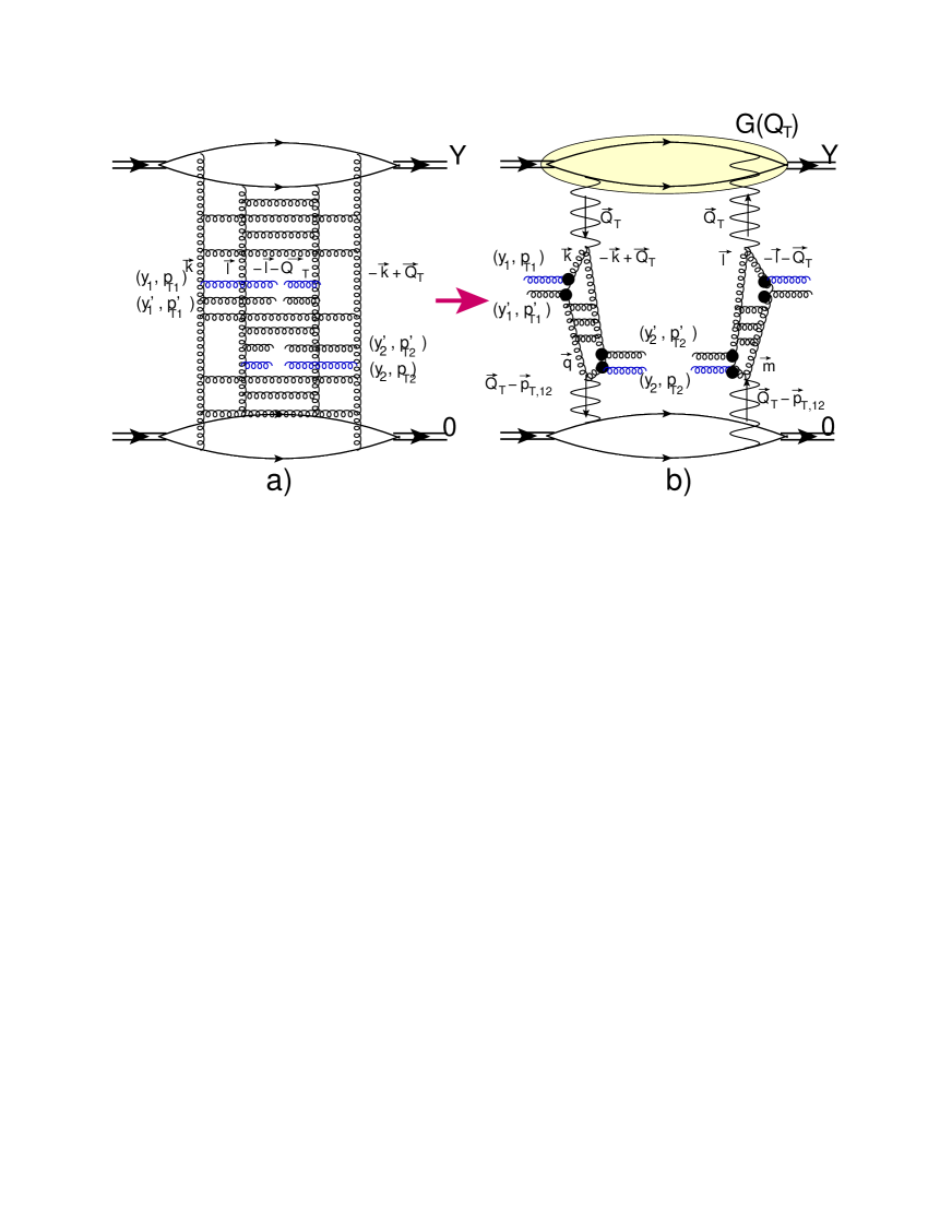
In Eq. (39) we use the following notation for ϕGN(Yy;QT=0;ki,kf)\phi^{N}_{G}\left(Y-y^{\prime};Q_{T}=0;k_{i},k_{f}\right): Yy𝑌superscript𝑦Y-y^{\prime} is the rapidity, QTsubscript𝑄𝑇Q_{T} is the momentum transfer of the BFKL Pomeron, kisubscript𝑘𝑖k_{i} and kfsubscript𝑘𝑓k_{f} are initial and final transverse momenta. Plugging Eq. (43) in the general expression for the interference diagram of Fig. 12-b, we see that instead of Eq. (34) we obtain

d2σdy1dy2d2pT1d2pT2(Fig.12b)=\displaystyle\frac{d^{2}\sigma}{dy_{1}\,dy_{2}d^{2}p_{T1}d^{2}p_{T2}}\left({Fig.~{}\ref{lmdiff}}-b\right)\,\,= (44)
12(2πα¯SCF)2d2QTGD(𝑸T𝒑T,12)dyϕGN(Yy;QT=0;qT,qT)d2qT\displaystyle\,\,\frac{1}{2}\left(\frac{2\pi\bar{\alpha}_{S}}{C_{F}}\right)^{2}\int d^{2}Q_{T}G_{D}\left(\boldsymbol{Q}_{T}-\boldsymbol{p}_{T,12}\right)\,\,\int\,d\,y^{\prime}\,\int\phi^{N}_{G}\left(Y-y^{\prime};Q_{T}=0;q_{T},q^{\prime}_{T}\right)\ d^{2}q^{\prime}_{T}
×\displaystyle\times (GBFKL(yy1;pT,12;𝒒T12𝒑T,12,kT)1kT2(𝒌T𝒑T,12)2(𝒌T𝒑T,1)4GBFKL(y2;0;𝒌T𝒑T1,kN)\displaystyle\Bigg{(}G^{\rm BFKL}\left(y^{\prime}-y_{1};p_{T,12};\boldsymbol{q^{\prime}}_{T}-\frac{1}{2}\boldsymbol{p}_{T,12},k_{T}\right)\,\,\frac{1}{k^{2}_{T}\,\left(\boldsymbol{k}_{T}-\boldsymbol{p}_{T,12}\right)^{2}\left(\boldsymbol{k}_{T}-\boldsymbol{p}_{T,1}\right)^{4}}G^{\rm BFKL}\left(y_{2};0;\boldsymbol{k}_{T}-\boldsymbol{p}_{T1},k_{N}\right)
×\displaystyle\times {(𝒌T𝒑T,12)2(𝒌T𝒑T,1)2pT22+kT2(𝒌T𝒑T,1𝒑T,12)2pT21pT,122pT,122kT2(𝒌T𝒑T,12)2pT21pT,22})\displaystyle\Bigg{\{}\frac{\left(\boldsymbol{k}_{T}-\boldsymbol{p}_{T,12}\right)^{2}\,\left(\boldsymbol{k}_{T}-\boldsymbol{p}_{T,1}\right)^{2}}{p^{2}_{T2}}\,+\,\frac{k^{2}_{T}\,\left(\boldsymbol{k}_{T}-\boldsymbol{p}_{T,1}-\boldsymbol{p}_{T,12}\right)^{2}}{p^{1}_{T2}}\,-\,p^{2}_{T,12}\,-\,p^{2}_{T,12}\frac{k^{2}_{T}\,\left(\boldsymbol{k}_{T}-\boldsymbol{p}_{T,12}\right)^{2}}{p^{1}_{T2}p^{2}_{T,2}}\Bigg{\}}\Bigg{)}
×\displaystyle\times (d2lTGBFKL(yy1;pT,12,𝒒T+12𝒑T,12,lT)1lT2(𝒍T+𝒑T,12)2(𝒍T𝒑T,2)4GBFKL(y2;0;𝒍T𝒑T2,lN)\displaystyle\,\Bigg{(}\int d^{2}l_{T}\,G^{\rm BFKL}\left(y^{\prime}-y_{1};p_{T,12},\boldsymbol{q^{\prime}}_{T}+\frac{1}{2}\boldsymbol{p}_{T,12},l_{T}\right)\,\,\frac{1}{l^{2}_{T}\,\left(\boldsymbol{l}_{T}+\boldsymbol{p}_{T,12}\right)^{2}\left(\boldsymbol{l}_{T}-\boldsymbol{p}_{T,2}\right)^{4}}G^{\rm BFKL}\left(y_{2};0;\boldsymbol{l}_{T}-\boldsymbol{p}_{T2},l_{N}\right)
×\displaystyle\times {(𝒍T+𝒑T,12)2(𝒍T𝒑T,1)2pT22+lT2(𝒍T𝒑T,2)2pT21pT,122pT,122lT2(𝒍T+𝒑T,12)2pT21pT,22})\displaystyle\Bigg{\{}\frac{\left(\boldsymbol{l}_{T}+\boldsymbol{p}_{T,12}\right)^{2}\,\left(\boldsymbol{l}_{T}-\boldsymbol{p}_{T,1}\right)^{2}}{p^{2}_{T2}}\,+\,\frac{l^{2}_{T}\,\left(\boldsymbol{l}_{T}-\boldsymbol{p}_{T,2}\right)^{2}}{p^{1}_{T2}}\,-\,p^{2}_{T,12}\,-\,p^{2}_{T,12}\frac{l^{2}_{T}\,\left(\boldsymbol{l}_{T}+\boldsymbol{p}_{T,12}\right)^{2}}{p^{1}_{T2}p^{2}_{T,2}}\Bigg{\}}\Bigg{)}

The main difference between Eq. (44) and Eq. (34), is that qTsubscriptsuperscript𝑞𝑇q^{\prime}_{T} is larger than qT 1/RNsubscript𝑞𝑇1subscript𝑅𝑁q_{T}\approx\,1/R_{N}. Indeed, the typical value of qT=Qs(Yy)(1/RN2)exp(λ(Yy))subscriptsuperscript𝑞𝑇subscript𝑄𝑠𝑌superscript𝑦similar-to1subscriptsuperscript𝑅2𝑁𝜆𝑌superscript𝑦q^{\prime}_{T}=Q_{s}\left(Y-y^{\prime}\right)\,\sim\left(1/R^{2}_{N}\right)\exp\left(\lambda\left(Y-y^{\prime}\right)\right), where λ=ω(γcr,0)/(1γcr\lambda=\omega\left(\gamma_{cr},0\right)/(1-\gamma_{cr} with γcr=0.37subscript𝛾𝑐𝑟0.37\gamma_{cr}=0.37 in leading order of perturbative QCD KOLEB ,

From Eq. (70) one can see that each ϕDN(Yy)eω(12,0)(Yy)proportional-tosubscriptsuperscriptitalic-ϕ𝑁𝐷𝑌superscript𝑦superscript𝑒𝜔120𝑌superscript𝑦\phi^{N}_{D}(Y-y^{\prime})\propto e^{\omega\left(\frac{1}{2},0\right)\,\left(Y-y^{\prime}\right)}, ϕDN(yy1)eω(12,0)(yy1)proportional-tosubscriptsuperscriptitalic-ϕ𝑁𝐷superscript𝑦subscript𝑦1superscript𝑒𝜔120superscript𝑦subscript𝑦1\phi^{N}_{D}(y^{\prime}-y_{1})\,\propto e^{\omega\left(\frac{1}{2},0\right)\,\left(y^{\prime}-y_{1}\right)}, and ϕDN(yy2)eω(12,0)(yy2)proportional-tosubscriptsuperscriptitalic-ϕ𝑁𝐷superscript𝑦subscript𝑦2superscript𝑒𝜔120superscript𝑦subscript𝑦2\phi^{N}_{D}(y^{\prime}-y_{2})\propto e^{\omega\left(\frac{1}{2},0\right)\,\left(y^{\prime}-y_{2}\right)}, since γ=12+iν𝛾12𝑖𝜈\gamma=\frac{1}{2}+i\nu with small ν𝜈\nu. Therefore, integration over ysuperscript𝑦y^{\prime} results in Yy1/ω(12,0)1/α¯Ssimilar-to𝑌superscript𝑦1𝜔120proportional-to1subscript¯𝛼𝑆Y-y^{\prime}\sim 1/\omega\left(\frac{1}{2},0\right)\propto 1/\bar{\alpha}_{S} while yy1superscript𝑦subscript𝑦1y^{\prime}-y_{1} and yy2superscript𝑦subscript𝑦2y^{\prime}-y_{2} are large (of the order of Y𝑌Y). Since Yyyy1much-less-than𝑌superscript𝑦superscript𝑦subscript𝑦1Y-y^{\prime}\ll y^{\prime}-y_{1}(Yyyy2much-less-than𝑌superscript𝑦superscript𝑦subscript𝑦2Y-y^{\prime}\ll y^{\prime}-y_{2}) we can use the factorized formula of Eq. (69) for ϕGN(yy1;pT,12;𝒒T12𝒑T,12,kT)subscriptsuperscriptitalic-ϕ𝑁𝐺superscript𝑦subscript𝑦1subscript𝑝𝑇12subscriptsuperscript𝒒bold-′𝑇12subscript𝒑𝑇12subscript𝑘𝑇\phi^{N}_{G}\left(y^{\prime}-y_{1};p_{T,12};\boldsymbol{q^{\prime}}_{T}-\frac{1}{2}\boldsymbol{p}_{T,12},k_{T}\right) and for ϕGN(yy1;pT,12,𝒒T+12𝒑T,12,lT)subscriptsuperscriptitalic-ϕ𝑁𝐺superscript𝑦subscript𝑦1subscript𝑝𝑇12subscriptsuperscript𝒒bold-′𝑇12subscript𝒑𝑇12subscript𝑙𝑇\phi^{N}_{G}\left(y^{\prime}-y_{1};p_{T,12},\boldsymbol{q^{\prime}}_{T}+\frac{1}{2}\boldsymbol{p}_{T,12},l_{T}\right). Using Eq. (69) we find that pT,12subscript𝑝𝑇12p_{T,12} will be determined by the lowest momenta in the BFKL Pomeron with yy1superscript𝑦subscript𝑦1y^{\prime}-y_{1}, and it will have the form

C(pT,12)d2qTIγ(qT)Vγ(𝒒T12𝑸T,𝑸T)Vγ(𝒒T+12𝑸T,𝑸T)proportional-to𝐶subscript𝑝𝑇12superscript𝑑2subscriptsuperscript𝑞𝑇subscript𝐼𝛾subscriptsuperscript𝑞𝑇subscript𝑉𝛾subscriptsuperscript𝒒bold-′𝑇12subscript𝑸𝑇subscript𝑸𝑇subscript𝑉𝛾subscriptsuperscript𝒒bold-′𝑇12subscript𝑸𝑇subscript𝑸𝑇C\left(p_{T,12}\right)\,\,\propto\,\,\int d^{2}q^{\prime}_{T}I_{-\gamma}\left(q^{\prime}_{T}\right)\,V_{\gamma}\left(\boldsymbol{q^{\prime}}_{T}-\frac{1}{2}\boldsymbol{Q}_{T},\boldsymbol{Q}_{T}\right)\,V_{\gamma}\left(\boldsymbol{q^{\prime}}_{T}+\frac{1}{2}\boldsymbol{Q}_{T},\boldsymbol{Q}_{T}\right) (45)

where V𝑉V is determined by Eq. (66), and QT=pT,12subscript𝑄𝑇subscript𝑝𝑇12Q_{T}=p_{T,12}. In Eq. (45) we can put γ=12𝛾12\gamma\,=\,\frac{1}{2}, assuming yy1superscript𝑦subscript𝑦1y^{\prime}-y_{1} is suffiently large, that we can neglect ν𝜈\nu.

IV Bose-Einstein correlation function in the nucleon-nucleon interaction

In this section we discuss the Bose-Einstein correlations in nucleon-nucleon scattering. The Mueller diagrams for the square of the diagrams Fig. 1-a and Fig. 1-b, and for the interference diagrams, are shown in Fig. 14. This differs from the diagrams that have been discussed above, only in the appearance of the second N(QT)𝑁subscript𝑄𝑇N\left(Q_{T}\right), which reflects the fact that we do not have small ( about 1/RD1subscript𝑅𝐷1/R_{D}) momenta in this process. Note, we can use perturbative QCD only if pT1pT21/RNsimilar-tosubscript𝑝𝑇1subscript𝑝𝑇2much-greater-than1subscript𝑅𝑁p_{T1}\sim p_{T2}\gg 1/R_{N}. Recalling that the QTsubscript𝑄𝑇Q_{T} dependence of the BFKL Pomeron is determined by the smallest transverse momentum, we conclude that in Fig. 14 the QTsubscript𝑄𝑇Q_{T} dependence is determined by the function N(QT)𝑁subscript𝑄𝑇N\left(Q_{T}\right). For the first two contributions to N(QT)𝑁subscript𝑄𝑇N\left(Q_{T}\right) (see Fig. 11-a), this is accurate to the order of 1/(RNpT1)1subscript𝑅𝑁subscript𝑝𝑇11/\left(R_{N}\,p_{T1}\right). For the third contribution of the large mass diffraction, the accuracy is about Qs/pT1subscript𝑄𝑠subscript𝑝𝑇1Q_{s}/p_{T1}, where Qssubscript𝑄𝑠Q_{s} denotes the saturation momentum of the BFKL Pomeron with rapidity Yy𝑌superscript𝑦Y-y^{\prime}.

In spite of the fact that we indicate in Fig. 11-a the sources of experimental information on each contribution, the situation turns out to be more complicated. As an example, we discuss the elastic contribution. This gives N(QT)=g2(QT)𝑁subscript𝑄𝑇superscript𝑔2subscript𝑄𝑇N\left(Q_{T}\right)=g^{2}\left(Q_{T}\right), where g(QT)𝑔subscript𝑄𝑇g\left(Q_{T}\right) is the Pomeron-hadron vertex. At first sight we can extract this vertex directly from the experimental values of dσel/dt𝑑subscript𝜎𝑒𝑙𝑑𝑡d\sigma_{el}/dt. However, this is certainly not correct. Indeed, the BFKL Pomeron cannot explain the shrinkage of the diffraction peak which is seen experimentally, and which gives almost a half of the slope of the elastic cross section for the energy range W=40 7000GeV𝑊407000𝐺𝑒𝑉W=40\,-\,7000\,GeVTOTEM . In the only modelGLM2CH for the soft interaction at high energy that is based on the BFKL Pomeron and Colour Glass Condensate (CGC) approachBK ; JIMWLK , the effective shrinkage of the diffraction peak stems from strong shadowing corrections, which lead to an elastic amplitude that is different from that for the exchange of the BFKL Pomeron. However, it turns out that the most essential shadowing corrections originate from the BFKL Pomeron interaction of two scattering hadrons. Such corrections do not contribute to the inclusive cross sections, as well as to the correlation due to AGK cutting rulesAGK .

It turns out to be an even more complicated problem to extract from the experimental data, the diffraction contribution to N(QT)𝑁subscript𝑄𝑇N\left(Q_{T}\right) in the region of small masses. The lack of a theory, as well as insufficient experimental data, especially of the momentum transfer distribution of the diffractively produced state with fixed mass, lead to the necessity of modeling this process. The two extreme cases of such a modeling illustrates the difficulties: in our model GLM2CH the rich variety of the produced states were replaced by a single state: and in the constituent quark modelCQM the small mass diffraction stems from production of the state of free three constituent quarks. In our model the typical slope for gdiff(QT)exp(BQT2)proportional-tosubscript𝑔𝑑𝑖𝑓𝑓subscript𝑄𝑇𝐵subscriptsuperscript𝑄2𝑇g_{diff}\left(Q_{T}\right)\propto\exp\left(-B\,Q^{2}_{T}\right) turns out to be 1/4 from the elastic slope, while in the CQM the size of the constituent quark is very small.
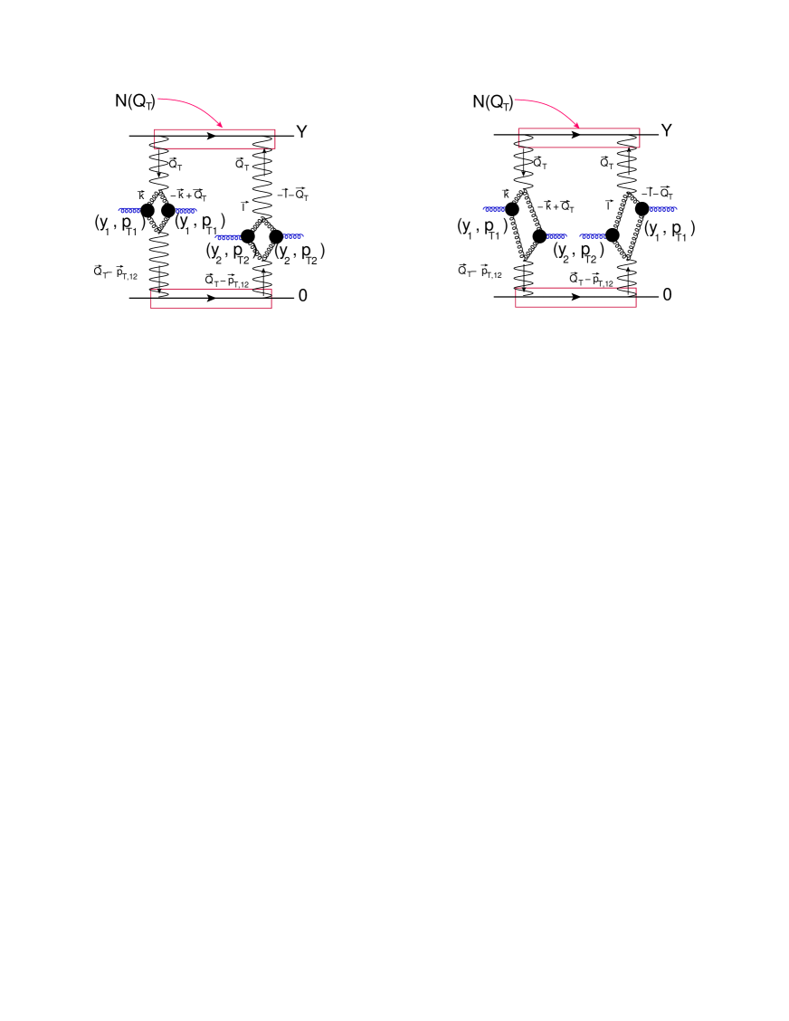
Refer to caption
Figure 14: The Mueller diagram for the double inclusive production of two gluons with rapidities y1subscript𝑦1y_{1} and y2subscript𝑦2y_{2} and transverse momenta 𝒑T1subscript𝒑𝑇1\boldsymbol{p}_{T1} and 𝒑T2subscript𝒑𝑇2\boldsymbol{p}_{T2} in the nucleon-nucleon interaction. The BFKL Pomerons are denoted by wavy lines. The first diagram corresponds to the square of the amplitude for two parton showers production, while the second diagram describes the interference.

Taking the above into consideration, the uncertainties in the large mass diffraction term look small, and for the triple BFKL Pomeron vertex, both the value and transverse momenta dependence follow directly from the Balitsky-Kovchegov equationBK . Bearing this in mind, we can write the expression for the interference diagram of Fig. 14, for the large mass diffraction contribution ( see Fig. 11). As we have discussed in this case QTQs(Yy)min{pT1(pT2),Qs(yy1)}similar-tosubscript𝑄𝑇subscript𝑄𝑠𝑌superscript𝑦much-less-thansubscript𝑝𝑇1subscript𝑝𝑇2subscript𝑄𝑠superscript𝑦subscript𝑦1Q_{T}\sim Q_{s}\left(Y-y^{\prime}\right)\,\,\ll\,\,\min\Big{\{}p_{T1}(p_{T2}),Q_{s}\left(y^{\prime}-y_{1}\right)\Big{\}}, |𝑸T𝒑T,12|Qs(Yy)min{pT1(pT2),Qs(yy1)}similar-tosubscript𝑸𝑇subscript𝒑𝑇12subscript𝑄𝑠𝑌superscript𝑦much-less-thansubscript𝑝𝑇1subscript𝑝𝑇2subscript𝑄𝑠superscript𝑦subscript𝑦1|\boldsymbol{Q}_{T}-\boldsymbol{p}_{T,12}|\sim\,Q_{s}\left(Y-y^{\prime}\right)\,\,\ll\,\,\min\Big{\{}p_{T1}(p_{T2}),Q_{s}\left(y^{\prime}-y_{1}\right)\Big{\}}, and kTmin{pT1(pT2),Qs(yy1)}similar-tosubscriptsuperscript𝑘𝑇subscript𝑝𝑇1subscript𝑝𝑇2subscript𝑄𝑠superscript𝑦subscript𝑦1k^{\prime}_{T}\sim\min\Big{\{}p_{T1}(p_{T2}),Q_{s}\left(y^{\prime}-y_{1}\right)\Big{\}} ( lTmin{pT1(pT2),Qs(yy1)}similar-tosubscriptsuperscript𝑙𝑇subscript𝑝𝑇1subscript𝑝𝑇2subscript𝑄𝑠superscript𝑦subscript𝑦1l^{\prime}_{T}\sim\min\Big{\{}p_{T1}(p_{T2}),Q_{s}\left(y^{\prime}-y_{1}\right)\Big{\}}). Hence, we can use the factorized form for ϕNGsubscriptsuperscriptitalic-ϕ𝐺𝑁\phi^{G}_{N} given by Eq. (69) and Eq. (70).

Finally, the large mass contribution for the interference diagram takes the form

d2σdy1dy2d2pT1d2pT2(Fig.14,interference diagram)=\displaystyle\frac{d^{2}\sigma}{dy_{1}\,dy_{2}d^{2}p_{T1}d^{2}p_{T2}}\left({Fig.~{}\ref{pppom}},\mbox{interference diagram}\right)\,\,=\,\,
121Nc21(2πα¯SCF)21pT12pT22dyϕGN(Yy;QT=0;qN,qT)\displaystyle\,\frac{1}{2}\frac{1}{N^{2}_{c}-1}\left(\frac{2\pi\bar{\alpha}_{S}}{C_{F}}\right)^{2}\frac{1}{p^{2}_{T1}\,p^{2}_{T2}}\,\,\int\,d\,y^{\prime}\,\int\phi^{N}_{G}\left(Y-y^{\prime};Q_{T}=0;q_{N},q^{\prime}_{T}\right)
d2qTd2kTGBFKL(yy1;QT;𝒒T12𝑸T,kT)𝑑y′′GBFKL(y2y′′;𝑸T𝒑T,12;𝒌T𝒑T1,𝒎T12(𝑸T𝒑T,12))superscript𝑑2subscriptsuperscript𝑞𝑇superscript𝑑2subscript𝑘𝑇superscript𝐺BFKLsuperscript𝑦subscript𝑦1subscript𝑄𝑇subscriptsuperscript𝒒bold-′𝑇12subscript𝑸𝑇subscript𝑘𝑇differential-dsuperscript𝑦′′superscript𝐺BFKLsubscript𝑦2superscript𝑦′′subscript𝑸𝑇subscript𝒑𝑇12subscript𝒌𝑇subscript𝒑𝑇1subscriptsuperscript𝒎𝑇12subscript𝑸𝑇subscript𝒑𝑇12\displaystyle\int d^{2}q^{\prime}_{T}\,d^{2}k_{T}G^{\rm BFKL}\left(y^{\prime}-y_{1};Q_{T};\boldsymbol{q^{\prime}}_{T}-\frac{1}{2}\boldsymbol{Q}_{T},k_{T}\right)\,\int dy^{\prime\prime}\,G^{\rm BFKL}\left(y_{2}-y^{\prime\prime};\boldsymbol{Q}_{T}-\boldsymbol{p}_{T,12};\boldsymbol{k}_{T}-\boldsymbol{p}_{T1},\boldsymbol{m}^{\prime}_{T}-\frac{1}{2}\left(\boldsymbol{Q}_{T}-\boldsymbol{p}_{T,12}\right)\right)
×d2lTd2mTGBFKL(yy1;QT,𝒒T+12𝑸T,lT)GBFKL(y2y′′;𝑸T𝒑T,12;𝒍T𝒑T2,𝒎T+12(𝑸T𝒑T,12))\displaystyle\times\,\,\int d^{2}l_{T}\,d^{2}m^{\prime}_{T}\,G^{\rm BFKL}\left(y^{\prime}-y_{1};Q_{T},\boldsymbol{q^{\prime}}_{T}+\frac{1}{2}\boldsymbol{Q}_{T},l_{T}\right)\,\,G^{\rm BFKL}\left(y_{2}-y^{\prime\prime};\boldsymbol{Q}_{T}-\boldsymbol{p}_{T,12};\boldsymbol{l}_{T}-\boldsymbol{p}_{T2},\boldsymbol{m}^{\prime}_{T}+\frac{1}{2}\left(\boldsymbol{Q}_{T}-\boldsymbol{p}_{T,12}\right)\right)
×ϕGN(y′′;QT=0;mN,mT)\displaystyle\times\,\,\phi^{N}_{G}\left(y^{\prime\prime};Q_{T}=0;m_{N},m^{\prime}_{T}\right) (46)

In the diagram for the square of the amplitude we can put 𝒑T,12=0subscript𝒑𝑇120\boldsymbol{p}_{T,12}=0. Thus, the correlation function with the correlation length of the order of 1/Qs(Yy)1subscript𝑄𝑠𝑌superscript𝑦1/Q_{s}\left(Y-y^{\prime}\right), takes the following form

C(pT,12/Qs)=121Nc21ND𝐶subscript𝑝𝑇12subscript𝑄𝑠121subscriptsuperscript𝑁2𝑐1𝑁𝐷C\left(p_{T,12}/Q_{s}\right)\,\,=\,\,\frac{1}{2}\frac{1}{N^{2}_{c}-1}\,\frac{N}{D} (47)

where

N=d2QTdyϕGN(Yy;QT=0;qN,qT)\displaystyle N\,=\,\,\,\int d^{2}Q_{T}\,\int\,d\,y^{\prime}\,\int\phi^{N}_{G}\left(Y-y^{\prime};Q_{T}=0;q_{N},q^{\prime}_{T}\right) (48)
d2qTd2kTGBFKL(yy1;QT;𝒒T12𝑸T,kT)𝑑y′′GBFKL(y2y′′;𝑸T𝒑T,12;𝒌T𝒑T1,𝒎T12(𝑸T𝒑T,12))superscript𝑑2subscriptsuperscript𝑞𝑇superscript𝑑2subscript𝑘𝑇superscript𝐺BFKLsuperscript𝑦subscript𝑦1subscript𝑄𝑇subscriptsuperscript𝒒bold-′𝑇12subscript𝑸𝑇subscript𝑘𝑇differential-dsuperscript𝑦′′superscript𝐺BFKLsubscript𝑦2superscript𝑦′′subscript𝑸𝑇subscript𝒑𝑇12subscript𝒌𝑇subscript𝒑𝑇1subscriptsuperscript𝒎𝑇12subscript𝑸𝑇subscript𝒑𝑇12\displaystyle\,\int d^{2}q^{\prime}_{T}\,d^{2}k_{T}G^{\rm BFKL}\left(y^{\prime}-y_{1};Q_{T};\boldsymbol{q^{\prime}}_{T}-\frac{1}{2}\boldsymbol{Q}_{T},k_{T}\right)\,\int dy^{\prime\prime}\,G^{\rm BFKL}\left(y_{2}-y^{\prime\prime};\boldsymbol{Q}_{T}-\boldsymbol{p}_{T,12};\boldsymbol{k}_{T}-\boldsymbol{p}_{T1},\boldsymbol{m}^{\prime}_{T}-\frac{1}{2}\left(\boldsymbol{Q}_{T}-\boldsymbol{p}_{T,12}\right)\right)
×\displaystyle\times d2lTd2mTGBFKL(yy1;QT,𝒒T+12𝑸T,lT)GBFKL(y2y′′;𝑸T𝒑T,12;𝒍T𝒑T2,𝒎T+12(𝑸T𝒑T,12))superscript𝑑2subscript𝑙𝑇superscript𝑑2subscriptsuperscript𝑚𝑇superscript𝐺BFKLsuperscript𝑦subscript𝑦1subscript𝑄𝑇subscriptsuperscript𝒒bold-′𝑇12subscript𝑸𝑇subscript𝑙𝑇superscript𝐺BFKLsubscript𝑦2superscript𝑦′′subscript𝑸𝑇subscript𝒑𝑇12subscript𝒍𝑇subscript𝒑𝑇2subscriptsuperscript𝒎𝑇12subscript𝑸𝑇subscript𝒑𝑇12\displaystyle\int d^{2}l_{T}\,d^{2}m^{\prime}_{T}\,G^{\rm BFKL}\left(y^{\prime}-y_{1};Q_{T},\boldsymbol{q^{\prime}}_{T}+\frac{1}{2}\boldsymbol{Q}_{T},l_{T}\right)\,\,G^{\rm BFKL}\left(y_{2}-y^{\prime\prime};\boldsymbol{Q}_{T}-\boldsymbol{p}_{T,12};\boldsymbol{l}_{T}-\boldsymbol{p}_{T2},\boldsymbol{m}^{\prime}_{T}+\frac{1}{2}\left(\boldsymbol{Q}_{T}-\boldsymbol{p}_{T,12}\right)\right)
×\displaystyle\times ϕGN(y′′;QT=0;mN,mT)\displaystyle\phi^{N}_{G}\left(y^{\prime\prime};Q_{T}=0;m_{N},m^{\prime}_{T}\right)

and

D=d2QTdyϕGN(Yy;QT=0;qN,qT)\displaystyle D\,=\,\,\,\int d^{2}Q_{T}\,\int\,d\,y^{\prime}\,\int\phi^{N}_{G}\left(Y-y^{\prime};Q_{T}=0;q_{N},q^{\prime}_{T}\right) (49)
d2qTd2kTϕGN(yy1;QT;𝒒T12𝑸T,kT)𝑑y′′ϕGN(y2y′′;𝑸T𝒑T,12;𝒌T𝒑T1,𝒎T12𝑸T)superscript𝑑2subscriptsuperscript𝑞𝑇superscript𝑑2subscript𝑘𝑇subscriptsuperscriptitalic-ϕ𝑁𝐺superscript𝑦subscript𝑦1subscript𝑄𝑇subscriptsuperscript𝒒bold-′𝑇12subscript𝑸𝑇subscript𝑘𝑇differential-dsuperscript𝑦′′subscriptsuperscriptitalic-ϕ𝑁𝐺subscript𝑦2superscript𝑦′′subscript𝑸𝑇subscript𝒑𝑇12subscript𝒌𝑇subscript𝒑𝑇1subscriptsuperscript𝒎𝑇12subscript𝑸𝑇\displaystyle\,\int d^{2}q^{\prime}_{T}\,d^{2}k_{T}\phi^{N}_{G}\left(y^{\prime}-y_{1};Q_{T};\boldsymbol{q^{\prime}}_{T}-\frac{1}{2}\boldsymbol{Q}_{T},k_{T}\right)\,\int dy^{\prime\prime}\,\phi^{N}_{G}\left(y_{2}-y^{\prime\prime};\boldsymbol{Q}_{T}-\boldsymbol{p}_{T,12};\boldsymbol{k}_{T}-\boldsymbol{p}_{T1},\boldsymbol{m}^{\prime}_{T}-\frac{1}{2}\boldsymbol{Q}_{T}\right)
×\displaystyle\times d2lTd2mTϕGN(yy1;QT,𝒒T+12𝑸T,lT)ϕGN(y2y′′;𝑸T;𝒍T,𝒎T+12𝑸T)superscript𝑑2subscript𝑙𝑇superscript𝑑2subscriptsuperscript𝑚𝑇subscriptsuperscriptitalic-ϕ𝑁𝐺superscript𝑦subscript𝑦1subscript𝑄𝑇subscriptsuperscript𝒒bold-′𝑇12subscript𝑸𝑇subscript𝑙𝑇subscriptsuperscriptitalic-ϕ𝑁𝐺subscript𝑦2superscript𝑦′′subscript𝑸𝑇subscript𝒍𝑇subscriptsuperscript𝒎𝑇12subscript𝑸𝑇\displaystyle\int d^{2}l_{T}\,d^{2}m^{\prime}_{T}\,\phi^{N}_{G}\left(y^{\prime}-y_{1};Q_{T},\boldsymbol{q^{\prime}}_{T}+\frac{1}{2}\boldsymbol{Q}_{T},l_{T}\right)\,\,\phi^{N}_{G}\left(y_{2}-y^{\prime\prime};\boldsymbol{Q}_{T};\boldsymbol{l}_{T},\boldsymbol{m}^{\prime}_{T}+\frac{1}{2}\boldsymbol{Q}_{T}\right)
×\displaystyle\times ϕGN(y′′;QT=0;mN,mT)\displaystyle\phi^{N}_{G}\left(y^{\prime\prime};Q_{T}=0;m_{N},m^{\prime}_{T}\right)

The rather long algebraic expression of Eq. (48) and Eq. (49) can be simplified using Eq. (71) and they take the following forms

N𝑁\displaystyle N\, =\displaystyle= d2QTdye2ω(12,0)yd2qTϕGN(Yy;QT=0;qN,qT)V12(𝒒𝑻,𝑸T12𝒑T,12)V12(𝒒𝑻,𝑸T+12𝒑T,12)|𝑸T12𝒑T,12||𝑸T+12𝒑T,12|\displaystyle\,\int d^{2}Q_{T}\,\int dy^{\prime}e^{2\omega\left(\frac{1}{2},0\right)\,y^{\prime}}\,d^{2}q^{\prime}_{T}\phi^{N}_{G}\left(Y-y^{\prime};Q_{T}=0;q_{N},q^{\prime}_{T}\right)\frac{V_{\frac{1}{2}}\left(\boldsymbol{q^{\prime}_{T}},\boldsymbol{Q}_{T}-\frac{1}{2}\boldsymbol{p}_{T,12}\right)\,V_{\frac{1}{2}}\left(\boldsymbol{q^{\prime}_{T}},\boldsymbol{Q}_{T}+\frac{1}{2}\boldsymbol{p}_{T,12}\right)}{|\boldsymbol{Q}_{T}-\frac{1}{2}\boldsymbol{p}_{T,12}|\,|\boldsymbol{Q}_{T}+\frac{1}{2}\boldsymbol{p}_{T,12}|} (50)
×\displaystyle\times dy′′e2ω(12,0)y′′d2lTϕGN(y′′;QT=0;lN,lT)V12(𝒍𝑻,𝑸T)V12(𝒍𝑻,𝑸T)QT2\displaystyle\,\,\int dy^{\prime\prime}e^{2\omega\left(\frac{1}{2},0\right)\,y^{\prime\prime}}\,d^{2}l^{\prime}_{T}\phi^{N}_{G}\left(y^{\prime\prime};Q_{T}=0;l_{N},l^{\prime}_{T}\right)\frac{V_{\frac{1}{2}}\left(\boldsymbol{l^{\prime}_{T}},\boldsymbol{Q}_{T}\right)\,V_{\frac{1}{2}}\left(\boldsymbol{l^{\prime}_{T}},\boldsymbol{Q}_{T}\right)}{Q^{2}_{T}}
D𝐷\displaystyle D\, =\displaystyle= d2QTdye2ω(12,0)yd2qTϕGN(Yy;QT=0;qN,qT)V12(𝒒𝑻,𝑸T)V12(𝒒𝑻,𝑸T)QT2\displaystyle\,\int d^{2}Q_{T}\,\int dy^{\prime}e^{2\omega\left(\frac{1}{2},0\right)\,y^{\prime}}\,d^{2}q^{\prime}_{T}\phi^{N}_{G}\left(Y-y^{\prime};Q_{T}=0;q_{N},q^{\prime}_{T}\right)\frac{V_{\frac{1}{2}}\left(\boldsymbol{q^{\prime}_{T}},\boldsymbol{Q}_{T}\right)\,V_{\frac{1}{2}}\left(\boldsymbol{q^{\prime}_{T}},\boldsymbol{Q}_{T}\right)}{Q^{2}_{T}} (51)
×\displaystyle\times dy′′e2ω(12,0)y′′d2lTϕGN(y′′;QT=0;lN,lT)V12(𝒍𝑻,𝑸T)V12(𝒍𝑻,𝑸T)QT2\displaystyle\,\,\int dy^{\prime\prime}e^{2\omega\left(\frac{1}{2},0\right)\,y^{\prime\prime}}\,d^{2}l^{\prime}_{T}\phi^{N}_{G}\left(y^{\prime\prime};Q_{T}=0;l_{N},l^{\prime}_{T}\right)\frac{V_{\frac{1}{2}}\left(\boldsymbol{l^{\prime}_{T}},\boldsymbol{Q}_{T}\right)\,V_{\frac{1}{2}}\left(\boldsymbol{l^{\prime}_{T}},\boldsymbol{Q}_{T}\right)}{Q^{2}_{T}}

V 𝜶¯𝑺(𝒚𝟏𝒚𝟐)  1much-greater-thansubscriptbold-¯𝜶𝑺subscript𝒚1subscript𝒚21\bar{\alpha}_{S}\left(y_{1}\,-\,y_{2}\right)\,\,\gg\,\,1

All our previous estimates were performed for small rapidity difference: α¯S|y1y2| 1subscript¯𝛼𝑆subscript𝑦1subscript𝑦21\bar{\alpha}_{S}|y_{1}-y_{2}|\,\leq\,1. In this section we discuss large rapidity differences (α¯S|y1y2| 1subscript¯𝛼𝑆subscript𝑦1subscript𝑦21\bar{\alpha}_{S}|y_{1}-y_{2}|\,\geq\,1). For simplicity, we consider only correlations with the typical length of the order of RDsubscript𝑅𝐷R_{D}. In other words, we discuss the generalization of Fig. 7 and Fig. 8 to the case of large y12=|y1y2|subscript𝑦12subscript𝑦1subscript𝑦2y_{12}=|y_{1}-y_{2}|. This generalization is shown in Fig. 15 for the interference diagrams. The new features here are that at rapidity y1<y1subscriptsuperscript𝑦1subscript𝑦1y^{\prime}_{1}<y_{1}, we need to emit an additional gluon, and integrate over both its rapidity (y1subscriptsuperscript𝑦1y^{\prime}_{1}) and its transferred momentum (pT1subscriptsuperscript𝑝𝑇1p^{\prime}_{T1}). Indeed, without this emission the ladder between rapidities y1subscriptsuperscript𝑦1y^{\prime}_{1} and y2subscriptsuperscript𝑦2y^{\prime}_{2} in Fig. 15-b will be in the octet state of color SU3𝑆subscript𝑈3SU_{3}. The main idea is, that the principle contribution stems from pT1pT1much-less-thansubscriptsuperscript𝑝𝑇1subscript𝑝𝑇1p^{\prime}_{T1}\ll p_{T1}. In this case the BFKL Pomeron between rapidities y1superscriptsubscript𝑦1y_{1}^{\prime} and y2subscriptsuperscript𝑦2y^{\prime}_{2} has the momentum transfer which is equal to pT1subscript𝑝𝑇1p_{T1}. After emission of two extra gluons with rapidities y2subscriptsuperscript𝑦2y^{\prime}_{2} and y2subscript𝑦2y_{2}, we obtain that the lower BFKL Pomeron, that has momentum transfer pT,12subscript𝑝𝑇12p_{T,12}, as in Fig. 8-b. In this diagram QT1/RDproportional-tosubscript𝑄𝑇1subscript𝑅𝐷Q_{T}\propto 1/R_{D}, and can be put equal to zero in all parts of the diagrams, except of G(QT)𝐺subscript𝑄𝑇G\left(Q_{T}\right) and G(𝑸T𝒑T,12)𝐺subscript𝑸𝑇subscript𝒑𝑇12G\left(\boldsymbol{Q}_{T}-\boldsymbol{p}_{T,12}\right).

Refer to caption
Figure 15: The double inclusive production of two gluons with rapidities y1subscript𝑦1y_{1} and y2subscript𝑦2y_{2} in the case of large |y1y2|subscript𝑦1subscript𝑦2|y_{1}-y_{2}| ( α¯S|y1y2| 1much-greater-thansubscript¯𝛼𝑆subscript𝑦1subscript𝑦21\bar{\alpha}_{S}\,|y_{1}-y_{2}|\,\gg\,1) and transverse momenta 𝒑T1subscript𝒑𝑇1\boldsymbol{p}_{T1} and 𝒑T2subscript𝒑𝑇2\boldsymbol{p}_{T2}, for the exchange of two BFKL Pomerons which are denoted by wavy lines. This diagram is the LLA generalization of Fig. 8. The solid lines denote nucleons in the deuterons, which are illustrated by double lines. Note, that the ladder, shown in Fig. 15-b, represents the BFKL Pomeron with the momentum transferred 𝒑T1+𝒑T1𝒑T1subscript𝒑𝑇1subscriptsuperscript𝒑𝑇1subscript𝒑𝑇1\boldsymbol{p}_{T1}+\boldsymbol{p}^{\prime}_{T1}\approx\boldsymbol{p}_{T1} for pT1pT2much-less-thansubscriptsuperscript𝑝𝑇1subscript𝑝𝑇2p^{\prime}_{T1}\ll p_{T2} (see the text).

First, we need to integrate over pT1subscriptsuperscript𝑝𝑇1p^{\prime}_{T1}. The vertex of the emission is shown in Fig. 16 which can be written as

α¯S2Γμ(𝒌T,𝒑T1)Γμ(𝒍T,𝒑T1)1kT2lT2Γν(𝒌T,𝒑T1)Γν(𝒍T,𝒑T1)1kT′′2lT′′2superscriptsubscript¯𝛼𝑆2subscriptΓ𝜇subscript𝒌𝑇subscript𝒑𝑇1subscriptΓ𝜇subscript𝒍𝑇subscript𝒑𝑇11subscriptsuperscript𝑘2𝑇subscriptsuperscript𝑙2𝑇subscriptΓ𝜈subscriptsuperscript𝒌𝑇subscript𝒑𝑇1subscriptΓ𝜈subscriptsuperscript𝒍𝑇subscript𝒑𝑇11subscriptsuperscript𝑘′′2𝑇subscriptsuperscript𝑙′′2𝑇\bar{\alpha}_{S}^{2}\,\Gamma_{\mu}\left(\boldsymbol{k}_{T},\boldsymbol{p}_{T1}\right)\,\Gamma_{\mu}\left(\boldsymbol{l}_{T},\boldsymbol{p}_{T1}\right)\,\frac{1}{k^{\prime 2}_{T}\,l^{\prime 2}_{T}}\Gamma_{\nu}\left(\boldsymbol{k}^{\prime}_{T},\boldsymbol{p}_{T1}\right)\,\Gamma_{\nu}\left(\boldsymbol{l}^{\prime}_{T},\boldsymbol{p}_{T1}\right)\,\frac{1}{k^{\prime\prime 2}_{T}\,l^{\prime\prime 2}_{T}} (52)

with 𝒌T=𝒌T𝒑T1subscriptsuperscript𝒌𝑇subscript𝒌𝑇subscript𝒑𝑇1\boldsymbol{k}^{\prime}_{T}=\boldsymbol{k}_{T}-\boldsymbol{p}_{T1} and 𝒌T′′=𝒌T𝒑T1=𝒌T𝒑T1𝒑T1subscriptsuperscript𝒌′′𝑇subscriptsuperscript𝒌𝑇subscriptsuperscript𝒑𝑇1subscript𝒌𝑇subscript𝒑𝑇1subscriptsuperscript𝒑𝑇1\boldsymbol{k}^{\prime\prime}_{T}=\boldsymbol{k}^{\prime}_{T}-\boldsymbol{p}^{\prime}_{T1}=\boldsymbol{k}_{T}-\boldsymbol{p}_{T1}-\boldsymbol{p}^{\prime}_{T1}. Plugging in Eq. (5),Eq. (6) andEq. (26) one can see that Eq. (52) takes the form

α¯S2d2pT11pT12{kT2kT2+lT2lT2pT12kT2lT2}1pT12{kT2kT′′2+lT2lT′′2pT12kT′′2lT′′2}superscriptsubscript¯𝛼𝑆2superscript𝑑2subscriptsuperscript𝑝𝑇11subscriptsuperscript𝑝2𝑇1subscriptsuperscript𝑘2𝑇subscriptsuperscript𝑘2𝑇subscriptsuperscript𝑙2𝑇subscriptsuperscript𝑙2𝑇subscriptsuperscript𝑝2𝑇1subscriptsuperscript𝑘2𝑇subscriptsuperscript𝑙2𝑇1subscriptsuperscript𝑝2𝑇1subscriptsuperscript𝑘2𝑇subscriptsuperscript𝑘′′2𝑇subscriptsuperscript𝑙2𝑇subscriptsuperscript𝑙′′2𝑇subscriptsuperscript𝑝2𝑇1subscriptsuperscript𝑘′′2𝑇subscriptsuperscript𝑙′′2𝑇\displaystyle\bar{\alpha}_{S}^{2}\,\int d^{2}p^{\prime}_{T1}\frac{1}{p^{2}_{T1}}\Bigg{\{}\frac{k^{2}_{T}}{k^{\prime 2}_{T}}\,+\,\frac{l^{2}_{T}}{l^{\prime 2}_{T}}\,-\,\frac{p^{2}_{T1}}{k^{\prime 2}_{T}\,l^{\prime 2}_{T}}\Bigg{\}}\,\frac{1}{p^{\prime 2}_{T1}}\Bigg{\{}\frac{k^{\prime 2}_{T}}{k^{\prime\prime 2}_{T}}\,+\,\frac{l^{\prime 2}_{T}}{l^{\prime\prime 2}_{T}}\,-\,\frac{p^{\prime 2}_{T1}}{k^{\prime\prime 2}_{T}\,l^{\prime\prime 2}_{T}}\Bigg{\}}\, (53)
pT1kT(lT) 2α¯S2kTd2pT1pT12[1pT12{kT2kT2+lT2lT2pT12kT2lT2}]=  2α¯S2min{kT,lT}d2pT1pT12K(𝒌T𝒍T,𝒌T,𝒌T)much-less-thansubscriptsuperscript𝑝𝑇1subscriptsuperscript𝑘𝑇subscriptsuperscript𝑙𝑇absent2superscriptsubscript¯𝛼𝑆2superscriptsubscriptsuperscript𝑘𝑇superscript𝑑2subscriptsuperscript𝑝𝑇1subscriptsuperscript𝑝2𝑇1delimited-[]1subscriptsuperscript𝑝2𝑇1subscriptsuperscript𝑘2𝑇subscriptsuperscript𝑘2𝑇subscriptsuperscript𝑙2𝑇subscriptsuperscript𝑙2𝑇subscriptsuperscript𝑝2𝑇1subscriptsuperscript𝑘2𝑇subscriptsuperscript𝑙2𝑇2superscriptsubscript¯𝛼𝑆2superscriptminsubscriptsuperscript𝑘𝑇subscriptsuperscript𝑙𝑇superscript𝑑2subscriptsuperscript𝑝𝑇1subscriptsuperscript𝑝2𝑇1𝐾subscript𝒌𝑇subscript𝒍𝑇subscript𝒌𝑇subscriptsuperscript𝒌𝑇\displaystyle\xrightarrow{p^{\prime}_{T1}\ll k^{\prime}_{T}(l^{\prime}_{T})}\,2\,\bar{\alpha}_{S}^{2}\,\int^{k^{\prime}_{T}}\frac{d^{2}p^{\prime}_{T1}}{p^{\prime 2}_{T1}}\left[\frac{1}{p^{2}_{T1}}\Bigg{\{}\frac{k^{2}_{T}}{k^{\prime 2}_{T}}\,+\,\frac{l^{2}_{T}}{l^{\prime 2}_{T}}\,-\,\frac{p^{2}_{T1}}{k^{\prime 2}_{T}\,l^{\prime 2}_{T}}\Bigg{\}}\right]\,\,=\,\,2\,\bar{\alpha}_{S}^{2}\,\int^{{\rm min}\{k^{\prime}_{T},l^{\prime}_{T}\}}\frac{d^{2}p^{\prime}_{T1}}{p^{\prime 2}_{T1}}\,K\left(\boldsymbol{k}_{T}-\boldsymbol{l}_{T},\boldsymbol{k}_{T},\boldsymbol{k}^{\prime}_{T}\right)

Note that the term []delimited-[]\Big{[}\dots\Big{]} is the same as in Fig. 8 and K(𝒌T𝒍T,𝒌T,𝒌T)𝐾subscript𝒌𝑇subscript𝒍𝑇subscript𝒌𝑇subscriptsuperscript𝒌𝑇K\left(\boldsymbol{k}_{T}-\boldsymbol{l}_{T},\boldsymbol{k}_{T},\boldsymbol{k}^{\prime}_{T}\right) is given by Eq. (26).

Refer to caption
Figure 16: The part of the diagram of Fig. 15-a with the vertex of emission of two gluons.

Finally, we obtain the following expression for the interference diagram of Fig. 16

d2σdy1dy2d2pT1d2pT2(Fig.15b)=  2(2πα¯SCF)2α¯S2d2QTGD(QT)GD(𝑸T𝒑T,12)\displaystyle\frac{d^{2}\sigma}{dy_{1}\,dy_{2}d^{2}p_{T1}d^{2}p_{T2}}\left({Fig.~{}\ref{ddipomlay}}-b\right)\,\,=\,\,2\left(\frac{2\pi\bar{\alpha}_{S}}{C_{F}}\right)^{2}\bar{\alpha}_{S}^{2}\int d^{2}Q_{T}G_{D}\left(Q_{T}\right)\,G_{D}\left(\boldsymbol{Q}_{T}-\boldsymbol{p}_{T,12}\right)
×d2kTd2lTϕGN(Yy1;𝒌T,𝒌T)ϕGN(Yy1;𝒍T,𝒍T)\displaystyle\times\,\int d^{2}k_{T}\,\,\int d^{2}l_{T}\,\,\phi^{N}_{G}\left(Y-y_{1};\boldsymbol{k}_{T},-\boldsymbol{k}_{T}\right)\,\,\phi^{N}_{G}\left(Y-y_{1};\boldsymbol{l}_{T},-\boldsymbol{l}_{T}\right)\,
min{kT,lT}y1𝑑y1d2pT1pT12K(𝒌T𝒍T,𝒌T,𝒌T)y2𝑑y2min{qT,mT}d2pT2pT22K(𝒒T𝒎T,𝒒T,𝒒T)superscriptminsubscriptsuperscript𝑘𝑇subscriptsuperscript𝑙𝑇superscriptsubscript𝑦1differential-dsubscriptsuperscript𝑦1superscript𝑑2subscriptsuperscript𝑝𝑇1subscriptsuperscript𝑝2𝑇1𝐾subscript𝒌𝑇subscript𝒍𝑇subscript𝒌𝑇subscriptsuperscript𝒌𝑇subscriptsubscript𝑦2differential-dsubscriptsuperscript𝑦2superscriptminsubscriptsuperscript𝑞𝑇subscriptsuperscript𝑚𝑇superscript𝑑2subscriptsuperscript𝑝𝑇2subscriptsuperscript𝑝2𝑇2𝐾subscript𝒒𝑇subscript𝒎𝑇subscript𝒒𝑇subscriptsuperscript𝒒𝑇\displaystyle\int^{{\rm min}\{k^{\prime}_{T},l^{\prime}_{T}\}}\int^{y_{1}}dy^{\prime}_{1}\,\frac{d^{2}p^{\prime}_{T1}}{p^{\prime 2}_{T1}}\,K\left(\boldsymbol{k}_{T}-\boldsymbol{l}_{T},\boldsymbol{k}_{T},\boldsymbol{k}^{\prime}_{T}\right)\int_{y_{2}}dy^{\prime}_{2}\,\int^{{\rm min}\{q^{\prime}_{T},m^{\prime}_{T}\}}\frac{d^{2}p^{\prime}_{T2}}{p^{\prime 2}_{T2}}\,K\left(\boldsymbol{q}_{T}-\boldsymbol{m}_{T},\boldsymbol{q}_{T},\boldsymbol{q}^{\prime}_{T}\right)
d2qTd2mTGBFKL(y1y2;𝒑T1;𝒌T𝒑T1,𝒒T+𝒑T2)GBFKL(y1y2;𝒑T1;𝒍T𝒑T1,𝒎T+𝒑T2)superscript𝑑2subscript𝑞𝑇superscript𝑑2subscript𝑚𝑇superscript𝐺BFKLsubscriptsuperscript𝑦1subscriptsuperscript𝑦2subscript𝒑𝑇1subscriptsuperscript𝒌bold-′𝑇subscriptsuperscript𝒑𝑇1subscriptsuperscript𝒒𝑇subscriptsuperscript𝒑𝑇2superscript𝐺BFKLsubscriptsuperscript𝑦1subscriptsuperscript𝑦2subscript𝒑𝑇1subscriptsuperscript𝒍𝑇subscriptsuperscript𝒑𝑇1subscriptsuperscript𝒎𝑇subscriptsuperscript𝒑𝑇2\displaystyle\int d^{2}q_{T}\int d^{2}m_{T}\,G^{\rm BFKL}\left(y^{\prime}_{1}-y^{\prime}_{2};\boldsymbol{p}_{T1};\boldsymbol{k^{\prime}}_{T}-\boldsymbol{p}^{\prime}_{T1},\boldsymbol{q}^{\prime}_{T}+\boldsymbol{p}^{\prime}_{T2}\right)G^{\rm BFKL}\left(y^{\prime}_{1}-y^{\prime}_{2};-\boldsymbol{p}_{T1};\boldsymbol{l}^{\prime}_{T}-\boldsymbol{p}^{\prime}_{T1},\boldsymbol{m}^{\prime}_{T}+\boldsymbol{p}^{\prime}_{T2}\right)
ϕGN(y2;𝒒T𝒑T1,𝒒T+𝒑T2)ϕGN(y2;𝒎T,𝒎T)subscriptsuperscriptitalic-ϕ𝑁𝐺subscript𝑦2subscript𝒒𝑇subscript𝒑𝑇1subscript𝒒𝑇subscript𝒑𝑇2subscriptsuperscriptitalic-ϕ𝑁𝐺subscript𝑦2subscript𝒎𝑇subscript𝒎𝑇\displaystyle\phi^{N}_{G}\left(y_{2};\boldsymbol{q}_{T}-\boldsymbol{p}_{T1},-\boldsymbol{q}_{T}+\boldsymbol{p}_{T2}\right)\,\phi^{N}_{G}\left(y_{2};\boldsymbol{m}_{T},-\boldsymbol{m}_{T}\right) (54)

In Eq. (V) we put QT=0subscript𝑄𝑇0Q_{T}=0 everywhere, except in GD(QT)subscript𝐺𝐷subscript𝑄𝑇G_{D}\left(Q_{T}\right) and GD(𝑸T𝒑T,12)subscript𝐺𝐷subscript𝑸𝑇subscript𝒑𝑇12G_{D}\left(\boldsymbol{Q}_{T}-\boldsymbol{p}_{T,12}\right), since QT 1/RDsimilar-tosubscript𝑄𝑇1subscript𝑅𝐷much-less-thanabsentQ_{T}\,\sim\,1/R_{D}\ll all other momenta. At first sight Eq. (V) gives the cross section which is suppressed as α¯S2superscriptsubscript¯𝛼𝑆2\bar{\alpha}_{S}^{2} in comparison with Eq. (III.1). However, the integration over y1subscriptsuperscript𝑦1y^{\prime}_{1} and y2subscriptsuperscript𝑦2y^{\prime}_{2} leads to 1/α¯S21superscriptsubscript¯𝛼𝑆21/\bar{\alpha}_{S}^{2} contributions, resulting in a cross section of the order of α¯S2superscriptsubscript¯𝛼𝑆2\bar{\alpha}_{S}^{2}. One can also see, that the cross section does not depend on the rapidity difference y12subscript𝑦12y_{12} for the large values of this difference.

The generalization to other cases, which we have considered above, is straightforward, and we not discuss it here.

VI Conclusions

VI.1 Comparison with other estimates in perturbative QCD

The first estimate of the azimuthal correlations due to the Bose-Einstein correlation in perturbative QCD, was performed in Ref.KOWE (see also Ref.KOLUCOR ). The diagrams, that were considered in these papers, are shown in Fig. 17-a. The observation is that these diagrams give rather strong azimuthal correlations, but they are symmetric with respect to ϕπϕitalic-ϕ𝜋italic-ϕ\phi\to\pi-\phi, and only generate vnsubscript𝑣𝑛v_{n} with even n𝑛n. The general origin of this symmetry was discussed in section II-B for slightly different diagrams. In Refs.KOWE ; KOLUCOR the QTsubscript𝑄𝑇Q_{T} dependence was neglected leading to δ𝛿\delta-function contributions, which were smeared out by QTsubscript𝑄𝑇Q_{T} dependance, with QT1/Rsimilar-tosubscript𝑄𝑇1𝑅Q_{T}\sim 1/R, where R𝑅R is the size of the interacting dipoles in Fig. 17-a.
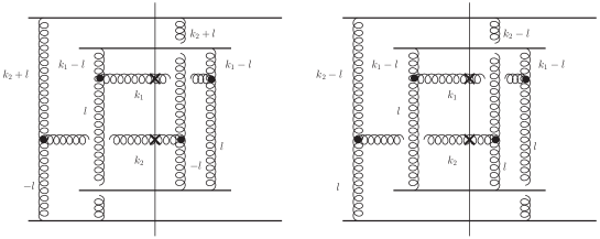
Refer to caption Refer to caption
Fig. 17-a Fig. 17-b
Figure 17: Fig. 17-a is taken from Ref.KOWE and describe the correlation in a one parton shower (see Fig. 17-b).

Since Fig. 17-a describes the production of two identical gluons in the dipole-dipole amplitude, in the Born approximation of perturbative QCD, these diagrams are responsible for the azimuthal correlations in one parton cascade shown in Fig. 17-b. It is worthwhile mentioning that the diagram of Fig. 17-a leads to a contribution which is proportional to exp(ω(12,0)y12)𝜔120subscript𝑦12\exp\left(-\omega\left(\frac{1}{2},0\right)\,y_{12}\right) and describes the correlations that decrease for large y12subscript𝑦12y_{12}. Therefore, only for ω(12,0)y121much-less-than𝜔120subscript𝑦121\omega\left(\frac{1}{2},0\right)\,y_{12}\ll 1, can we consider this diagram as a source of correlations which are independent of y12subscript𝑦12y_{12}.

Refer to caption
Figure 18: The generalized diagram of Fig. 17-a, taking into account the gluon emission (two parton shower contribution).

Taking into account the emission of gluons, we can generalize the diagram of Fig. 17-a to the diagram of Fig. 18. We have considered this diagram above, and have shown that there is no symmetry with respect of ϕπϕitalic-ϕ𝜋italic-ϕ\phi\to\pi-\phi in such diagrams. Therefore, we conclude that the symmetry ϕπϕitalic-ϕ𝜋italic-ϕ\phi\to\pi-\phi, is a feature of the azimuthal correlations in the one parton shower, in the Born approximation of perturbative QCD.

VI.2 Summary

In this paper, we found within the framework of perturbative QCD, that the Bose-Einstein correlations due to two parton shower production, induce azimuthal angle correlations, with three correlation lengths: the size of the deuteron, the proton radius, and the size of the BFKL Pomeron which is closely related to the saturation momentum (Rc1/Qssimilar-tosubscript𝑅𝑐1subscript𝑄𝑠R_{c}\sim 1/Q_{s}). These correlations are independent of the values of rapidities of produced gluons (long range rapidity correlations), and have no symmetry with respect to ϕπϕitalic-ϕ𝜋italic-ϕ\phi\to\pi-\phi (𝒑T1𝒑T1subscript𝒑𝑇1subscript𝒑𝑇1\boldsymbol{p}_{T1}\to-\boldsymbol{p}_{T1}). Therefore, they give rise to vnsubscript𝑣𝑛v_{n} for all values of n𝑛n, not only even values.

We reproduce the result of Refs.KOWE ; KOLUCOR which show this symmetry in the Born approximation of perturbative QCD. However, even in the Born approximation, this symmetry depends on the amplitude of the gluon - nucleon interaction at large distances, of about the nucleon size and, therefore, it inherently has a non-perturbative nature. Replacing the nucleon by an onium: the quark-antiquark bound state of heavy quarks, we see that symmetry ϕπϕitalic-ϕ𝜋italic-ϕ\phi\to\pi-\phi (𝒑T1𝒑T1subscript𝒑𝑇1subscript𝒑𝑇1\boldsymbol{p}_{T1}\to-\boldsymbol{p}_{T1}), does not hold for distances of the order of the size of the onium.

We demonstrated that the azimuthal correlations with the correlation length (Rcsubscript𝑅𝑐R_{c}) of about the size of the deuteron, and the size of nucleon, stem from a non-perturbative contribution, and their estimates demand a lot of modeling due to the embryonic state of the theory in the non-perturbative region. However, the correlations with Rc1/Qssimilar-tosubscript𝑅𝑐1subscript𝑄𝑠R_{c}\sim 1/Q_{s} have a perturbative origin, and can be evaluated in the framework of the Colour Gluon Condensate (CGC) approach.

We show that the two parton showers contributions, generate long range rapidity azimuthal angle correlations, which intuitively have been expected. In other words, we demonstrate that the azimuthal angle correlations do not depend on y12=|y1y2|subscript𝑦12subscript𝑦1subscript𝑦2y_{12}=|y_{1}-y_{2}| for large values of y12subscript𝑦12y_{12} (α¯Sy12 1subscript¯𝛼𝑆subscript𝑦121\bar{\alpha}_{S}\,y_{12}\,\geq\,1). We illustrate that the correlation of Refs.KOWE ; KOLUCOR , actually describe the correlations in a one parton shower, and can be viewed, as independent of the rapidity difference, only in the narrow rapidity window α¯Sy121much-less-thansubscript¯𝛼𝑆subscript𝑦121\bar{\alpha}_{S}y_{12}\ll 1.

Acknowledgements We thank our colleagues at Tel Aviv University and UTFSM for encouraging discussions. Our special thanks go to Carlos Cantreras, Alex Kovner and Michel Lublinsky for elucidating discussions on the subject of this paper.

This research was supported by the BSF grant 2012124, by Proyecto Basal FB 0821(Chile) , Fondecyt (Chile) grant 1140842, and by CONICYT grant PIA ACT1406.

Appendix A 𝑸𝑻subscript𝑸𝑻Q_{T} dependence of the BFKL Pomeron

The impact parameter dependence of the BFKL Pomeron is well knownLI , and it has the following form for the scattering of two dipoles (r1subscript𝑟1r_{1} and r2subscript𝑟2r_{2} ) at impact parameter b𝑏bLI ; NAPE :

NIP(r1,r2;Y,b)=dγ2πieω(γ,0)YHγ(w,w)subscript𝑁𝐼𝑃subscript𝑟1subscript𝑟2𝑌𝑏𝑑𝛾2𝜋𝑖superscript𝑒𝜔𝛾0𝑌superscript𝐻𝛾𝑤superscript𝑤N_{I\!\!P}\left(r_{1},r_{2};Y,b\right)\,\,=\,\,\int\frac{d\gamma}{2\,\pi\,i}\,e^{\omega(\gamma,0)\,Y}\,H^{\gamma}\left(w,w^{*}\right) (55)

where

ω(γ,0)=α¯S(2ψ(1)ψ(γ)ψ(1γ))𝜔𝛾0subscript¯𝛼𝑆2𝜓1𝜓𝛾𝜓1𝛾\omega(\gamma,0)\,\,=\,\,\bar{\alpha}_{S}\left(2\psi(1)-\psi(\gamma)-\psi(1-\gamma)\right) (56)

and where ψ(z)𝜓𝑧\psi(z) is the Euler ψ(z)=dlnΓ(z)/dz𝜓𝑧𝑑Γ𝑧𝑑𝑧\psi(z)=d\ln\Gamma\left(z\right)/dz (digamma function) (see Ref.RY formula 8.360 - 8.367).

Hγ(w,w)superscript𝐻𝛾𝑤superscript𝑤\displaystyle H^{\gamma}\left(w,w^{*}\right)\,\, \displaystyle\equiv (γ12)2(γ(1γ))2{bγwγwγF(γ,γ,2γ,w)F(γ,γ,2γ,w)+\displaystyle\,\frac{(\gamma-\frac{1}{2})^{2}}{(\gamma(1-\gamma))^{2}}\Bigg{\{}b_{\gamma}\,w^{\gamma}\,{w^{*}}^{\gamma}\,F\left(\gamma,\gamma,2\gamma,w\right)\,F\left(\gamma,\gamma,2\gamma,w^{*}\right)\,+ (57)
b1γw1γw1γF(1γ,1γ,22γ,w)F(1γ,1γ,22γ,w)}\displaystyle b_{1-\gamma}w^{1-\gamma}{w^{*}}^{1-\gamma}F\left(1-\gamma,1-\gamma,2-2\gamma,w\right)\,F\left(1-\gamma,1-\gamma,2-2\gamma,w^{*}\right)\Bigg{\}}
ww 1much-less-than𝑤superscript𝑤1\displaystyle\xrightarrow{w\,w^{*}\,\ll\,1} (γ12)2(γ(1γ))2{bγwγwγ+b1γw1γw1γ}superscript𝛾122superscript𝛾1𝛾2subscript𝑏𝛾superscript𝑤𝛾superscriptsuperscript𝑤𝛾subscript𝑏1𝛾superscript𝑤1𝛾superscriptsuperscript𝑤1𝛾\displaystyle\,\frac{(\gamma-\frac{1}{2})^{2}}{(\gamma(1-\gamma))^{2}}\Bigg{\{}b_{\gamma}\,w^{\gamma}\,{w^{*}}^{\gamma}\,\,+\,b_{1-\gamma}w^{1-\gamma}{w^{*}}^{1-\gamma}\Bigg{\}} (58)

where FF12𝐹subscriptsubscript𝐹12F\,\equiv\,{}_{2}F_{1} is hypergeometric function RY . In Eq. (57) ww𝑤superscript𝑤w\,w^{*} is equal to

ww=r12r22(𝒃12(𝒓1𝒓2))2(𝒃+12(𝒓1𝒓2))2𝑤superscript𝑤subscriptsuperscript𝑟21subscriptsuperscript𝑟22superscript𝒃12subscript𝒓1subscript𝒓22superscript𝒃12subscript𝒓1subscript𝒓22w\,w^{*}\,\,=\,\,\frac{r^{2}_{1}\,r^{2}_{2}}{\left(\boldsymbol{b}-\frac{1}{2}\left(\,\boldsymbol{r}_{1}\,-\,\boldsymbol{r}_{2}\right)\right)^{2}\,\left(\boldsymbol{b}\,+\,\frac{1}{2}\left(\,\boldsymbol{r}_{1}\,-\,\boldsymbol{r}_{2}\right)\right)^{2}} (59)

and bγsubscript𝑏𝛾b_{\gamma} is given by

bγ=π3 24(1/2γ)Γ(γ)Γ(1/2γ)Γ(1γ)Γ(1/2+γ).subscript𝑏𝛾superscript𝜋3superscript2412𝛾Γ𝛾Γ12𝛾Γ1𝛾Γ12𝛾b_{\gamma}\,=\,\pi^{3}\,2^{4(1/2-\gamma)}\,\frac{\Gamma\left(\gamma\right)}{\Gamma\left(1/2-\gamma\right)}\,\frac{\Gamma\left(1-\gamma\right)}{\Gamma\left(1/2+\gamma\right)}. (60)

From Eq. (57) and Eq. (59) we see that (i) b𝑏b is about of the size of the largest dipole (br2similar-to𝑏subscript𝑟2b\sim r_{2} for r2r1much-greater-thansubscript𝑟2subscript𝑟1r_{2}\gg r_{1}); and (ii) the scattering amplitude has a symmetry with respect to 𝒃𝒃𝒃𝒃\boldsymbol{b}\,\to\,-\boldsymbol{b}. QTsubscript𝑄𝑇Q_{T} is the conjugated variable to b𝑏b, since

NIP(r1,r2;b;Y)=r12r22d2kd2kei𝒌T𝒓1+i𝒌T𝒓2d2QTei𝑸T𝒃GBFKL(Y;QT;kT,kT)subscript𝑁𝐼𝑃subscript𝑟1subscript𝑟2𝑏𝑌subscriptsuperscript𝑟21subscriptsuperscript𝑟22superscript𝑑2𝑘superscript𝑑2superscript𝑘superscript𝑒𝑖subscript𝒌𝑇subscript𝒓1𝑖subscriptsuperscript𝒌bold-′𝑇subscript𝒓2superscript𝑑2subscript𝑄𝑇superscript𝑒𝑖subscript𝑸𝑇𝒃superscript𝐺BFKL𝑌subscript𝑄𝑇subscriptsuperscript𝑘𝑇subscript𝑘𝑇N_{I\!\!P}\left(r_{1},r_{2};b;Y\right)\,\,=\,\,r^{2}_{1}r^{2}_{2}\int d^{2}k\,d^{2}k^{\prime}e^{i\boldsymbol{k}_{T}\cdot\boldsymbol{r}_{1}\,+\,i\boldsymbol{k^{\prime}}_{T}\cdot\boldsymbol{r}_{2}}\int d^{2}Q_{T}\,e^{i\boldsymbol{Q}_{T}\cdot\boldsymbol{b}}\,G^{\rm BFKL}\left(Y;Q_{T};k^{\prime}_{T},k_{T}\right)\, (61)

we see that the value of typical QT1/r21/RNproportional-tosubscript𝑄𝑇1subscript𝑟21subscript𝑅𝑁Q_{T}\propto 1/r_{2}\approx 1/R_{N}. In Eq. (61) GBFKL(yy;QT;kT,kT)superscript𝐺BFKL𝑦superscript𝑦subscript𝑄𝑇subscriptsuperscript𝑘𝑇subscript𝑘𝑇G^{\rm BFKL}\left(y-y^{\prime};Q_{T};k^{\prime}_{T},k_{T}\right) denotes the BFKL Pomeron Green’s function with the momentum transferred QTsubscript𝑄𝑇Q_{T}, and the transverse momenta of gluons kTsubscript𝑘𝑇k_{T} at y and kTsubscriptsuperscript𝑘𝑇k^{\prime}_{T} at y’. The initial condition for the BFKL Green’s function is the exchange of two gluons at y=y𝑦superscript𝑦y=y^{\prime}.

In Eq. (61), the value of r1subscript𝑟1r_{1} in our problem, is about 1/pT11subscript𝑝𝑇11/p_{T1} or 1/pT21subscript𝑝𝑇21/p_{T2}, and we trust perturbative QCD calculations only if pT1pT2 1/RNsimilar-tosubscript𝑝𝑇1subscript𝑝𝑇2much-greater-than1subscript𝑅𝑁p_{T1}\sim p_{T2}\,\gg\,1/R_{N}. Since r1r2much-less-thansubscript𝑟1subscript𝑟2r_{1}\ll r_{2} we can use Eq. (58) and take ww𝑤superscript𝑤w\,w^{*} to be equal to

ww=r12r22(𝒃12𝒓2)2(𝒃+12𝒓2)2𝑤superscript𝑤subscriptsuperscript𝑟21subscriptsuperscript𝑟22superscript𝒃12subscript𝒓22superscript𝒃12subscript𝒓22w\,w^{*}\,\,=\,\,\frac{r^{2}_{1}\,r^{2}_{2}}{\left(\boldsymbol{b}-\frac{1}{2}\boldsymbol{r}_{2}\right)^{2}\,\left(\boldsymbol{b}\,+\,\frac{1}{2}\boldsymbol{r}_{2}\right)^{2}} (62)

Bearing in mind that

Iγ(𝒌)=d2r(r2)γei𝒌𝒓=  212γΓ(1γ)Γ(γ)1(k2)1γsubscript𝐼𝛾𝒌superscript𝑑2𝑟superscriptsuperscript𝑟2𝛾superscript𝑒𝑖𝒌𝒓superscript212𝛾Γ1𝛾Γ𝛾1superscriptsuperscript𝑘21𝛾I_{\gamma}\left(\boldsymbol{k}\right)\,\,=\,\,\int\frac{d^{2}r}{\left(r^{2}\right)^{\gamma}}\,e^{i\boldsymbol{k}\cdot\boldsymbol{r}}\,\,=\,\,2^{1-2\gamma}\frac{\Gamma\left(1-\gamma\right)}{\Gamma\left(\gamma\right)}\frac{1}{\left(k^{2}\right)^{1-\gamma}} (63)

Plugging Eq. (63) in Eq. (61) we obtain

GBFKL(γ;𝑸T;𝒌T,𝒌T)=(γ12)2(γ(1γ))2superscript𝐺BFKL𝛾subscript𝑸𝑇subscriptsuperscript𝒌bold-′𝑇subscript𝒌𝑇superscript𝛾122superscript𝛾1𝛾2\displaystyle G^{\rm BFKL}\left(\gamma;\boldsymbol{Q}_{T};\boldsymbol{k^{\prime}}_{T},\boldsymbol{k}_{T}\right)\,\,=\,\,\frac{\left(\gamma-\frac{1}{2}\right)^{2}}{\left(\gamma(1-\gamma)\right)^{2}} (64)
×\displaystyle\times {bγd2mTI1γ(𝒌T𝒎T)Iγ(𝒎12𝑸T)Iγ(𝒎+12𝑸T)I1γ(𝒌T)\displaystyle\Bigg{\{}b_{\gamma}\,\int d^{2}m^{\prime}_{T}I_{1-\gamma}\left(\boldsymbol{k^{\prime}}_{T}-\boldsymbol{m^{\prime}}_{T}\right)\,I_{\gamma}\left(\boldsymbol{m^{\prime}}-\frac{1}{2}\boldsymbol{Q}_{T}\right)\,I_{\gamma}\left(\boldsymbol{m^{\prime}}+\frac{1}{2}\boldsymbol{Q}_{T}\right)\,I_{1-\gamma}\left(\boldsymbol{k}_{T}\right)\,
+\displaystyle+ b1γd2mTIγ(𝒌T𝒎T)I1γ(𝒎12𝑸T)I1γ(𝒎+12𝑸T)Iγ(𝒌T)}}\displaystyle\,b_{1-\gamma}\int d^{2}m_{T}I_{\gamma}\left(\boldsymbol{k^{\prime}}_{T}-\boldsymbol{m}_{T}\right)\,I_{1-\gamma}\left(\boldsymbol{m}-\frac{1}{2}\boldsymbol{Q}_{T}\right)\,I_{1-\gamma}\left(\boldsymbol{m}+\frac{1}{2}\boldsymbol{Q}_{T}\right)\,I_{\gamma}\left(\boldsymbol{k}_{T}\right)\}\Bigg{\}}\,

The integrals over msuperscript𝑚m^{\prime} can be taken by replacing vector variables by the complex coordinatesLI

𝒌ρk=kx+iky;ρk=kxiky;formulae-sequence𝒌subscript𝜌𝑘subscript𝑘𝑥𝑖subscript𝑘𝑦subscriptsuperscript𝜌𝑘subscript𝑘𝑥𝑖subscript𝑘𝑦\boldsymbol{k}\,\,\to\,\,\rho_{k}\,=\,k_{x}\,+\,i\,k_{y};~{}~{}~{}~{}~{}~{}\rho^{*}_{k}\,=\,k_{x}\,-\,i\,k_{y}; (65)

where kxsubscript𝑘𝑥k_{x} and kysubscript𝑘𝑦k_{y} denote the x𝑥x and y𝑦y projections of 𝒌𝒌\boldsymbol{k}. Using formula 3.197(1) of Ref.RY we can take integrals over d2m=dρmdρmsuperscript𝑑2superscript𝑚𝑑subscript𝜌superscript𝑚𝑑subscriptsuperscript𝜌superscript𝑚d^{2}m^{\prime}\,=\,d\rho_{m^{\prime}}\,d\rho^{*}_{m^{\prime}}:

Vγ(𝒌𝑻,𝑸T)=d2mTI1γ(𝒌T𝒎T)Iγ(𝒎12𝑸T)Iγ(𝒎+12𝑸T)=subscript𝑉𝛾subscriptsuperscript𝒌bold-′𝑻subscript𝑸𝑇superscript𝑑2subscriptsuperscript𝑚𝑇subscript𝐼1𝛾subscriptsuperscript𝒌bold-′𝑇subscriptsuperscript𝒎bold-′𝑇subscript𝐼𝛾superscript𝒎bold-′12subscript𝑸𝑇subscript𝐼𝛾superscript𝒎bold-′12subscript𝑸𝑇absent\displaystyle V_{\gamma}\left(\boldsymbol{k^{\prime}_{T}},\boldsymbol{Q}_{T}\right)\,=\,\int d^{2}m^{\prime}_{T}I_{1-\gamma}\left(\boldsymbol{k^{\prime}}_{T}-\boldsymbol{m^{\prime}}_{T}\right)\,I_{\gamma}\left(\boldsymbol{m^{\prime}}-\frac{1}{2}\boldsymbol{Q}_{T}\right)\,I_{\gamma}\left(\boldsymbol{m^{\prime}}+\frac{1}{2}\boldsymbol{Q}_{T}\right)\,=
dρmdρmI1γ((ρkρm(ρkρm))Iγ((ρm+12ρQ)(ρm+12ρQ))Iγ((ρm12ρQ)(ρm12ρQ))\displaystyle\,\int d\rho_{m^{\prime}}\,d\rho^{*}_{m^{\prime}}I_{1-\gamma}\left((\rho_{k}-\rho_{m^{\prime}}(\rho^{*}_{k}-\rho^{*}_{m^{\prime}})\right)\,I_{\gamma}\left((\rho_{m^{\prime}}+\frac{1}{2}\rho_{Q})(\rho^{*}_{m^{\prime}}+\frac{1}{2}\rho^{*}_{Q})\right)\,I_{\gamma}\left((\rho_{m^{\prime}}-\frac{1}{2}\rho_{Q})(\rho^{*}_{m^{\prime}}-\frac{1}{2}\rho^{*}_{Q})\right)
= 224γΓ4(1γ)1((𝒌T12𝑸T)2)γ1(QT2)12γF(γ,γ,1,ρk+12ρQρk12ρQ)F(γ,γ,1,ρk+12ρQρk12ρQ)absentsuperscript224𝛾superscriptΓ41𝛾1superscriptsuperscriptsubscript𝒌𝑇12subscript𝑸𝑇2𝛾1superscriptsubscriptsuperscript𝑄2𝑇12𝛾𝐹𝛾𝛾1subscript𝜌𝑘12subscript𝜌𝑄subscript𝜌𝑘12subscript𝜌𝑄𝐹𝛾𝛾1subscriptsuperscript𝜌𝑘12subscriptsuperscript𝜌𝑄subscriptsuperscript𝜌𝑘12subscriptsuperscript𝜌𝑄\displaystyle=\,2^{2-4\gamma}\Gamma^{4}\left(1-\gamma\right)\,\frac{1}{\left(\left(\boldsymbol{k}_{T}-\frac{1}{2}\boldsymbol{Q}_{T}\right)^{2}\right)^{\gamma}}\,\frac{1}{\left(Q^{2}_{T}\right)^{1-2\gamma}}\,F\left(\gamma,\gamma,1,\frac{\rho_{k}+\frac{1}{2}\rho_{Q}}{\rho_{k}-\frac{1}{2}\rho_{Q}}\right)\,\,F\left(\gamma,\gamma,1,\frac{\rho^{*}_{k}+\frac{1}{2}\rho^{*}_{Q}}{\rho^{*}_{k}-\frac{1}{2}\rho^{*}_{Q}}\right) (66)
=(9.131(1) of Ref.RY ) 224γΓ4(1γ)1(QT2)γF(γ,1γ,1,ρk+ρQρQ)F(γ,1γ,1,ρk+ρQρQ)absent(9.131(1) of Ref.RY )superscript224𝛾superscriptΓ41𝛾1superscriptsubscriptsuperscript𝑄2𝑇𝛾𝐹𝛾1𝛾1subscript𝜌𝑘subscript𝜌𝑄subscript𝜌𝑄𝐹𝛾1𝛾1subscriptsuperscript𝜌𝑘subscriptsuperscript𝜌𝑄subscriptsuperscript𝜌𝑄\displaystyle=~{}~{}\mbox{\Bigg{(}{\bf 9.131(1)} of Ref.\cite[cite]{\@@bibref{Authors Phrase1YearPhrase2}{RY}{\@@citephrase{(}}{\@@citephrase{)}}}\Bigg{)}}~{}~{}\,2^{2-4\gamma}\Gamma^{4}\left(1-\gamma\right)\frac{1}{\left(Q^{2}_{T}\right)^{\gamma}}\,F\left(\gamma,1-\gamma,1,\frac{\rho_{k}+\rho_{Q}}{\rho_{Q}}\right)\,F\left(\gamma,1-\gamma,1,\frac{\rho^{*}_{k}+\rho^{*}_{Q}}{\rho^{*}_{Q}}\right) (67)
=(9.132(2) of Ref.RY )  224γΓ4(1γ)1((𝒌T+𝑸T)2)γabsent(9.132(2) of Ref.RY )superscript224𝛾superscriptΓ41𝛾1superscriptsuperscriptsubscript𝒌𝑇subscript𝑸𝑇2𝛾\displaystyle=~{}~{}\mbox{\Bigg{(}{\bf 9.132(2)} of Ref.\cite[cite]{\@@bibref{Authors Phrase1YearPhrase2}{RY}{\@@citephrase{(}}{\@@citephrase{)}}}\Bigg{)}}~{}~{}\,\,2^{2-4\gamma}\Gamma^{4}\left(1-\gamma\right)\frac{1}{\left(\left(\boldsymbol{k}_{T}+\boldsymbol{Q}_{T}\right)^{2}\right)^{\gamma}} (68)
×{Γ(12γ)Γ2(1γ)F(γ,γ,2γ,ρQρk+ρQ)+(ρQρk+ρQ)12γΓ(1+2γ)Γ2(1γ)F(1γ,1γ,2(1γ),ρQρk+ρQ)}absentΓ12𝛾superscriptΓ21𝛾𝐹𝛾𝛾2𝛾subscript𝜌𝑄subscript𝜌𝑘subscript𝜌𝑄superscriptsubscript𝜌𝑄subscript𝜌𝑘subscript𝜌𝑄12𝛾Γ12𝛾superscriptΓ21𝛾𝐹1𝛾1𝛾21𝛾subscript𝜌𝑄subscript𝜌𝑘subscript𝜌𝑄\displaystyle\,\times\Bigg{\{}\frac{\Gamma\left(1-2\gamma\right)}{\Gamma^{2}\left(1-\gamma\right)}F\left(\gamma,\gamma,2\gamma,\frac{\rho_{Q}}{\rho_{k}+\rho_{Q}}\right)\,+\,\left(\frac{\rho_{Q}}{\rho_{k}+\rho_{Q}}\right)^{1-2\gamma}\,\frac{\Gamma\left(-1+2\gamma\right)}{\Gamma^{2}\left(1\gamma\right)}F\left(1-\gamma,1-\gamma,2(1-\gamma),\frac{\rho_{Q}}{\rho_{k}+\rho_{Q}}\right)\Bigg{\}}
×{Γ(12γ)Γ2(1γ)F(γ,γ,2γ,ρQρk+ρQ)+(ρQρk+ρQ)12γΓ(1+2γ)Γ2(1γ)F(1γ,1γ,2(1γ),ρQρk+ρQ)}\displaystyle\times\Bigg{\{}\frac{\Gamma\left(1-2\gamma\right)}{\Gamma^{2}\left(1-\gamma\right)}F\left(\gamma,\gamma,2\gamma,\frac{\rho^{*}_{Q}}{\rho^{*}_{k}+\rho^{*}_{Q}}\right)\,+\,\left(\frac{\rho^{*}_{Q}}{\rho^{*}_{k}+\rho^{*}_{Q}}\right)^{1-2\gamma}\,\frac{\Gamma\left(-1+2\gamma\right)}{\Gamma^{2}\left(1\gamma\right)}F\left(1-\gamma,1-\gamma,2(1-\gamma),\frac{\rho*_{Q}}{\rho^{*}_{k}+\rho^{*}_{Q}}\right)\Bigg{\}}

Plugging Eq. (65) in Eq. (64) one can see that ϕGN(γ,𝒌T,𝒌T,𝑸T)subscriptsuperscriptitalic-ϕ𝑁𝐺𝛾subscriptsuperscript𝒌bold-′𝑇subscript𝒌𝑇subscript𝑸𝑇\phi^{N}_{G}\left(\gamma,\boldsymbol{k^{\prime}}_{T},\boldsymbol{k}_{T},\boldsymbol{Q}_{T}\right) can be written in the factorized form:

GBFKL(γ;𝑸T;𝒌T,𝒌T)=Vγ(𝒌𝑻,𝑸T)Iγ(𝒌T)+V1γ(𝒌𝑻,𝑸T)I1γ(𝒌T)superscript𝐺BFKL𝛾subscript𝑸𝑇subscriptsuperscript𝒌bold-′𝑇subscript𝒌𝑇subscript𝑉𝛾subscriptsuperscript𝒌bold-′𝑻subscript𝑸𝑇subscript𝐼𝛾subscript𝒌𝑇subscript𝑉1𝛾subscriptsuperscript𝒌bold-′𝑻subscript𝑸𝑇subscript𝐼1𝛾subscript𝒌𝑇G^{\rm BFKL}\left(\gamma;\boldsymbol{Q}_{T};\boldsymbol{k^{\prime}}_{T},\boldsymbol{k}_{T}\right)\,=\,V_{\gamma}\left(\boldsymbol{k^{\prime}_{T}},\boldsymbol{Q}_{T}\right)\,I_{\gamma}\left(\boldsymbol{k}_{T}\right)\,\,+\,\,V_{1-\gamma}\left(\boldsymbol{k^{\prime}_{T}},\boldsymbol{Q}_{T}\right)\,I_{1-\gamma}\left(\boldsymbol{k}_{T}\right) (69)

ϕGNsubscriptsuperscriptitalic-ϕ𝑁𝐺\phi^{N}_{G} in the rapidity representation can be calculated as

GBFKL(Y;,𝑸T;𝒌T,𝒌T)=ϵiϵ+idγ2πieω(γ,0)YGBFKL(γ,𝒌T,𝒌T,𝑸T)G^{\rm BFKL}\left(Y;,\boldsymbol{Q}_{T};\boldsymbol{k^{\prime}}_{T},\boldsymbol{k}_{T}\right)\,\,=\,\,\int^{\epsilon+i\infty}_{\epsilon-i\infty}\frac{d\gamma}{2\pi i}\,e^{\omega\left(\gamma,0\right)Y}\,G^{\rm BFKL}\left(\gamma,\boldsymbol{k^{\prime}}_{T},\boldsymbol{k}_{T},\boldsymbol{Q}_{T}\right) (70)

Taking the integral over γ𝛾\gamma in Eq. (70) by the method of steepest descend KOLEB , we see that for large Y1much-greater-than𝑌1Y\gg 1 the essential γ=12+iν𝛾12𝑖𝜈\gamma=\frac{1}{2}+i\nu, where ν𝜈\nu is small. Bearing this in mind, we can see from Eq. (67) that at large QTkTmuch-greater-thansubscript𝑄𝑇subscriptsuperscript𝑘𝑇Q_{T}\gg k^{\prime}_{T}, GBFKL(Y;,𝑸T;𝒌T,𝒌T)  1/(QT2)γ1/QTG^{\rm BFKL}\left(Y;,\boldsymbol{Q}_{T};\boldsymbol{k^{\prime}}_{T},\boldsymbol{k}_{T}\right)\,\propto\,\,1/\left(Q^{2}_{T}\right)^{\gamma}\approx 1/Q_{T}. At QT0subscript𝑄𝑇0Q_{T}\to 0 QTkTmuch-greater-thansubscript𝑄𝑇subscriptsuperscript𝑘𝑇Q_{T}\gg k^{\prime}_{T} GBFKL(Y;,𝑸T;𝒌T,𝒌T)G^{\rm BFKL}\left(Y;,\boldsymbol{Q}_{T};\boldsymbol{k^{\prime}}_{T},\boldsymbol{k}_{T}\right)\,\to\, Const. Therefore, we conclude that the typical value QTsubscript𝑄𝑇Q_{T} in the BFKL Pomeron, is about kTsubscriptsuperscript𝑘𝑇k^{\prime}_{T}: the smallest transverse momenta.

At large Y𝑌Y we can simplify Eq. (70) using Eq. (69) and the small size of ν𝜈\nu. Plugging GBFKL(Y;,𝑸T;𝒌T,𝒌T)G^{\rm BFKL}\left(Y;,\boldsymbol{Q}_{T};\boldsymbol{k^{\prime}}_{T},\boldsymbol{k}_{T}\right) from Eq. (69) in Eq. (70), we have

GBFKL(Y;𝑸T;𝒌T,𝒌T)superscript𝐺BFKL𝑌subscript𝑸𝑇subscriptsuperscript𝒌bold-′𝑇subscript𝒌𝑇\displaystyle G^{\rm BFKL}\left(Y;\boldsymbol{Q}_{T};\boldsymbol{k^{\prime}}_{T},\boldsymbol{k}_{T}\right)\,\, =\displaystyle= ϵiϵ+idγ2πieω(γ,0)Y 2V12+iν(𝒌𝑻,𝑸T)Iγ(𝒌T)subscriptsuperscriptitalic-ϵ𝑖italic-ϵ𝑖𝑑𝛾2𝜋𝑖superscript𝑒𝜔𝛾0𝑌2subscript𝑉12𝑖𝜈subscriptsuperscript𝒌bold-′𝑻subscript𝑸𝑇subscript𝐼𝛾subscript𝒌𝑇\displaystyle\,\,\int^{\epsilon+i\infty}_{\epsilon-i\infty}\frac{d\gamma}{2\pi i}\,e^{\omega\left(\gamma,0\right)Y}\,2\,V_{\frac{1}{2}+i\nu}\left(\boldsymbol{k^{\prime}_{T}},\boldsymbol{Q}_{T}\right)\,I_{\gamma}\left(\boldsymbol{k}_{T}\right)\, (71)
ν1much-less-than𝜈1\displaystyle\xrightarrow{\nu\ll 1} 2C(γ=12)kTkTV12(𝒌𝑻,𝑸T)+iϵ++iϵdν2πe(ω(12,0)Dν2)Y+iνln(kT2/kT2)2𝐶𝛾12subscriptsuperscript𝑘𝑇subscript𝑘𝑇subscript𝑉12subscriptsuperscript𝒌bold-′𝑻subscript𝑸𝑇subscriptsuperscript𝑖italic-ϵ𝑖italic-ϵ𝑑𝜈2𝜋superscript𝑒𝜔120𝐷superscript𝜈2𝑌𝑖𝜈subscriptsuperscript𝑘2𝑇subscriptsuperscript𝑘2𝑇\displaystyle\,\,\frac{2\,C\left(\gamma=\frac{1}{2}\right)}{k^{\prime}_{T}\,k_{T}}V_{\frac{1}{2}}\left(\boldsymbol{k^{\prime}_{T}},\boldsymbol{Q}_{T}\right)\int^{+\infty+i\epsilon}_{-\infty+i\epsilon}\frac{d\nu}{2\pi}\,\,e^{\left(\omega\left(\frac{1}{2},0\right)\,-\,D\,\nu^{2}\right)\,Y\,+i\nu\ln\left(k^{2}_{T}/k^{\prime 2}_{T}\right)}
=\displaystyle= 2C(γ=12)kTkTV12(𝒌𝑻,𝑸T)(2πDYeω(12,0)Yln2(kT2/kT2)4DY)2𝐶𝛾12subscriptsuperscript𝑘𝑇subscript𝑘𝑇subscript𝑉12subscriptsuperscript𝒌bold-′𝑻subscript𝑸𝑇2𝜋𝐷𝑌superscript𝑒𝜔120𝑌superscript2subscriptsuperscript𝑘2𝑇subscriptsuperscript𝑘2𝑇4𝐷𝑌\displaystyle\,\,\frac{2\,C\left(\gamma=\frac{1}{2}\right)}{k^{\prime}_{T}\,k_{T}}V_{\frac{1}{2}}\left(\boldsymbol{k^{\prime}_{T}},\boldsymbol{Q}_{T}\right)\Bigg{(}\sqrt{\frac{2\pi}{D\,Y}}\,e^{\omega\left(\frac{1}{2},0\right)\,Y\,-\,\frac{\ln^{2}\left(k^{\prime 2}_{T}/k^{2}_{T}\right)}{4\,D\,Y}}\Bigg{)}

Integral in Eq. (71) is taken in the saddle point approximation with νSP=iln(kT2/kT2)/2DY  1subscript𝜈𝑆𝑃𝑖subscriptsuperscript𝑘2𝑇subscriptsuperscript𝑘2𝑇2𝐷𝑌much-less-than1\nu_{SP}=i\ln\left(k^{2}_{T}/k^{\prime 2}_{T}\right)/2\,D\,Y\,\,\ll\,\,1 and ω(12=iν,0)=ω(12,0)Dν2𝜔12𝑖𝜈0𝜔120𝐷superscript𝜈2\omega\left(\frac{1}{2}=i\nu,0\right)\,\,=\,\,\omega\left(\frac{1}{2},0\right)\,\,-\,\,D\,\nu^{2}.

Appendix B The BFKL Pomeron - onium vertex

The scattering amplitude of a dipole of size x01subscript𝑥01x_{01} with an onium has the following form:

A(Y,x01;QT)=d2x01ei𝒙01𝑸TΨonium(x01)N(Y;x01,x01,QT)Ψonium(x01)𝐴𝑌subscript𝑥01subscript𝑄𝑇superscript𝑑2subscriptsuperscript𝑥01superscript𝑒𝑖subscriptsuperscript𝒙bold-′01subscript𝑸𝑇subscriptsuperscriptΨoniumsubscriptsuperscript𝑥01𝑁𝑌subscriptsuperscript𝑥01subscript𝑥01subscript𝑄𝑇subscriptsuperscriptΨoniumsubscriptsuperscript𝑥01A\left(Y,x_{01};Q_{T}\right)\,\,=\,\,\int d^{2}x^{\prime}_{01}\,e^{i\boldsymbol{x^{\prime}}_{01}\cdot\boldsymbol{Q}_{T}}\,\Psi^{*}_{\rm onium}\left(x^{\prime}_{01}\right)\,N\left(Y;x^{\prime}_{01},x_{01},Q_{T}\right)\,\Psi^{*}_{\rm onium}\left(x^{\prime}_{01}\right) (72)

In the momentum representation it can be written as

A(γ,kT,kT,QT)=(F(QT)F(2𝒌T𝑸T))d2x01ei𝒌T𝒙01i𝒌T𝒙01N(γ;x01,x01,QT)/x012𝐴𝛾subscriptsuperscript𝑘𝑇subscript𝑘𝑇subscript𝑄𝑇𝐹subscript𝑄𝑇𝐹2subscriptsuperscript𝒌bold-′𝑇subscript𝑸𝑇superscript𝑑2subscriptsuperscript𝑥01superscript𝑒𝑖subscriptsuperscript𝒌bold-′𝑇subscriptsuperscript𝒙bold-′01𝑖subscript𝒌𝑇subscript𝒙01𝑁𝛾subscriptsuperscript𝑥01subscript𝑥01subscript𝑄𝑇subscriptsuperscript𝑥201A\left(\gamma,k^{\prime}_{T},k_{T},Q_{T}\right)\,=\,\left(F\left(Q_{T}\right)-F\left(2\boldsymbol{k^{\prime}}_{T}-\boldsymbol{Q}_{T}\right)\right)\int d^{2}x^{\prime}_{01}e^{-i\boldsymbol{k^{\prime}}_{T}\cdot\boldsymbol{x^{\prime}}_{01}-i\boldsymbol{k}_{T}\cdot\boldsymbol{x}_{01}}\,N\left(\gamma;x^{\prime}_{01},x_{01},Q_{T}\right)/x^{2}_{01} (73)

The amplitude ei𝒌T𝒙01i𝒌T𝒙01N(γ;x01,x01,QT)/x012superscript𝑒𝑖subscriptsuperscript𝒌bold-′𝑇subscriptsuperscript𝒙bold-′01𝑖subscript𝒌𝑇subscript𝒙01𝑁𝛾subscriptsuperscript𝑥01subscript𝑥01subscript𝑄𝑇subscriptsuperscript𝑥201e^{-i\boldsymbol{k^{\prime}}_{T}\cdot\boldsymbol{x^{\prime}}_{01}-i\boldsymbol{k}_{T}\cdot\boldsymbol{x}_{01}}\,N\left(\gamma;x^{\prime}_{01},x_{01},Q_{T}\right)/x^{2}_{01} can be written in the factorized form of Eq. (69):

ei𝒌T𝒙01i𝒌T𝒙01N(γ;x01,x01,QT)/x012=Vγpr(𝒌𝑻,𝑸T)Nγ(𝒌T)+V1γpr(𝒌𝑻,𝑸T)N1γ(𝒌T)superscript𝑒𝑖subscriptsuperscript𝒌bold-′𝑇subscriptsuperscript𝒙bold-′01𝑖subscript𝒌𝑇subscript𝒙01𝑁𝛾subscriptsuperscript𝑥01subscript𝑥01subscript𝑄𝑇subscriptsuperscript𝑥201subscriptsuperscript𝑉pr𝛾subscriptsuperscript𝒌bold-′𝑻subscript𝑸𝑇subscript𝑁𝛾subscript𝒌𝑇subscriptsuperscript𝑉pr1𝛾subscriptsuperscript𝒌bold-′𝑻subscript𝑸𝑇subscript𝑁1𝛾subscript𝒌𝑇e^{-i\boldsymbol{k^{\prime}}_{T}\cdot\boldsymbol{x^{\prime}}_{01}-i\boldsymbol{k}_{T}\cdot\boldsymbol{x}_{01}}\,N\left(\gamma;x^{\prime}_{01},x_{01},Q_{T}\right)/x^{2}_{01}\,\,=\,\,\,V^{\rm pr}_{\gamma}\left(\boldsymbol{k^{\prime}_{T}},\boldsymbol{Q}_{T}\right)\,N_{\gamma}\left(\boldsymbol{k}_{T}\right)\,\,+\,\,V^{\rm pr}_{1-\gamma}\left(\boldsymbol{k^{\prime}_{T}},\boldsymbol{Q}_{T}\right)\,N_{1-\gamma}\left(\boldsymbol{k}_{T}\right) (74)

where Vγpr(𝒌𝑻,𝑸T)subscriptsuperscript𝑉pr𝛾subscriptsuperscript𝒌bold-′𝑻subscript𝑸𝑇V^{\rm pr}_{\gamma}\left(\boldsymbol{k^{\prime}_{T}},\boldsymbol{Q}_{T}\right) is equal to

Vγpr(𝒌𝑻,𝑸T)=d2mTIγ(𝒌T𝒎T)Iγ(𝒎12𝑸T)Iγ(𝒎+12𝑸T)=subscriptsuperscript𝑉pr𝛾subscriptsuperscript𝒌bold-′𝑻subscript𝑸𝑇superscript𝑑2subscriptsuperscript𝑚𝑇subscript𝐼𝛾subscriptsuperscript𝒌bold-′𝑇subscriptsuperscript𝒎bold-′𝑇subscript𝐼𝛾superscript𝒎bold-′12subscript𝑸𝑇subscript𝐼𝛾superscript𝒎bold-′12subscript𝑸𝑇absent\displaystyle V^{\rm pr}_{\gamma}\left(\boldsymbol{k^{\prime}_{T}},\boldsymbol{Q}_{T}\right)\,=\,\int d^{2}m^{\prime}_{T}I_{-\gamma}\left(\boldsymbol{k^{\prime}}_{T}-\boldsymbol{m^{\prime}}_{T}\right)\,I_{\gamma}\left(\boldsymbol{m^{\prime}}-\frac{1}{2}\boldsymbol{Q}_{T}\right)\,I_{\gamma}\left(\boldsymbol{m^{\prime}}+\frac{1}{2}\boldsymbol{Q}_{T}\right)\,= (75)
dρmdρmIγ((ρkρm(ρkρm))Iγ((ρm+12ρQ)(ρm+12ρQ))Iγ((ρm12ρQ)(ρm12ρQ))\displaystyle\,\int d\rho_{m^{\prime}}\,d\rho^{*}_{m^{\prime}}I_{-\gamma}\left((\rho_{k}-\rho_{m^{\prime}}(\rho^{*}_{k}-\rho^{*}_{m^{\prime}})\right)\,I_{\gamma}\left((\rho_{m^{\prime}}+\frac{1}{2}\rho_{Q})(\rho^{*}_{m^{\prime}}+\frac{1}{2}\rho^{*}_{Q})\right)\,I_{\gamma}\left((\rho_{m^{\prime}}-\frac{1}{2}\rho_{Q})(\rho^{*}_{m^{\prime}}-\frac{1}{2}\rho^{*}_{Q})\right)
= 232γΓ(1+γ)Γ2(1γ)Γ(γ)Γ2(γ)1((𝒌T12𝑸T)2)1+γ1(QT2)12γF(1+γ,γ,2,ρk+12ρQρk12ρQ)F(1+γ,γ,2,ρk+12ρQρk12ρQ)absentsuperscript232𝛾Γ1𝛾superscriptΓ21𝛾Γ𝛾superscriptΓ2𝛾1superscriptsuperscriptsubscript𝒌𝑇12subscript𝑸𝑇21𝛾1superscriptsubscriptsuperscript𝑄2𝑇12𝛾𝐹1𝛾𝛾2subscript𝜌𝑘12subscript𝜌𝑄subscript𝜌𝑘12subscript𝜌𝑄𝐹1𝛾𝛾2subscriptsuperscript𝜌𝑘12subscriptsuperscript𝜌𝑄subscriptsuperscript𝜌𝑘12subscriptsuperscript𝜌𝑄\displaystyle=\,2^{3-2\gamma}\frac{\Gamma\left(1+\gamma\right)\Gamma^{2}\left(1-\gamma\right)}{\Gamma\left(-\gamma\right)\,\Gamma^{2}\left(\gamma\right)}\,\frac{1}{\left(\left(\boldsymbol{k}_{T}-\frac{1}{2}\boldsymbol{Q}_{T}\right)^{2}\right)^{1+\gamma}}\,\frac{1}{\left(Q^{2}_{T}\right)^{1-2\gamma}}\,F\left(1+\gamma,\gamma,2,\frac{\rho_{k}+\frac{1}{2}\rho_{Q}}{\rho_{k}-\frac{1}{2}\rho_{Q}}\right)\,\,F\left(1+\gamma,\gamma,2,\frac{\rho^{*}_{k}+\frac{1}{2}\rho^{*}_{Q}}{\rho^{*}_{k}-\frac{1}{2}\rho^{*}_{Q}}\right)

Finally, the BFKL Pomeron-onium vertex takes the form

Vγonium(QT)=d2kT(F(QT)F(2𝒌T𝑸T))Vγpr(𝒌𝑻,𝑸T)subscriptsuperscript𝑉onium𝛾subscript𝑄𝑇superscript𝑑2subscriptsuperscript𝑘𝑇𝐹subscript𝑄𝑇𝐹2subscriptsuperscript𝒌bold-′𝑇subscript𝑸𝑇subscriptsuperscript𝑉pr𝛾subscriptsuperscript𝒌bold-′𝑻subscript𝑸𝑇V^{\rm onium}_{\gamma}\left(Q_{T}\right)\,=\,\int d^{2}k^{\prime}_{T}\left(F\left(Q_{T}\right)-F\left(2\boldsymbol{k^{\prime}}_{T}-\boldsymbol{Q}_{T}\right)\right)\,V^{\rm pr}_{\gamma}\left(\boldsymbol{k^{\prime}_{T}},\boldsymbol{Q}_{T}\right) (76)

References

  • (1) E. M. Levin, M. G. Ryskin and S. I. Troian, Sov. J. Nucl. Phys.  23 (1976) 222 [Yad. Fiz.  23 (1976) 423];     A. Capella, A. Krzywicki and E. M. Levin, Phys. Rev. D 44 (1991) 704.
  • (2) Y. V. Kovchegov and D. E. Wertepny, Nucl. Phys. A 906 (2013) 50, [arXiv:1212.1195 [hep-ph]];   
  • (3) T. Altinoluk, N. Armesto, G. Beuf, A. Kovner and M. Lublinsky, Phys. Lett. B 752 (2016) 113, [arXiv:1509.03223 [hep-ph]];    T. Altinoluk, N. Armesto, G. Beuf, A. Kovner and M. Lublinsky, Phys. Lett. B 751 (2015) 448, [arXiv:1503.07126 [hep-ph]].
  • (4) E. Gotsman, E. Levin and U. Maor, “Bose-Einstein correlations and 𝐯𝟐𝐧subscript𝐯2𝐧\mathbf{v_{2n}} and 𝐯𝟐𝐧𝟏subscript𝐯2𝐧1\mathbf{v_{2n-1}} in hadron and nucleus collisions,” arXiv:1604.04461 [hep-ph];    “CGC/saturation approach for high energy soft interactions: ‘soft’ Pomeron structure and vnsubscript𝑣𝑛v_{n} in hadron and nucleus collisions from Bose-Einstein correlation,” arXiv:1607.00594 [hep-ph].
  • (5) V. Khachatryan et al. [CMS Collaboration], arXiv:1510.03068 [nucl-ex];  JHEP 1009 (2010) 091 [arXiv:1009.4122 [hep-ex]]. arXiv:1510.03068 [nucl-ex].
  • (6) J. Adams et al. [STAR Collaboration], Phys. Rev. Lett.  95 (2005) 152301 [nucl-ex/0501016].
  • (7) B. Alver et al. [PHOBOS Collaboration], Phys. Rev. Lett.  104 (2010) 062301 [arXiv:0903.2811 [nucl-ex]].
  • (8) H. Agakishiev et al. [STAR Collaboration], arXiv:1010.0690 [nucl-ex].
  • (9) S. Chatrchyan et al. [CMS Collaboration], Phys. Lett. B 718 (2013) 795 [arXiv:1210.5482 [nucl-ex]];    V. Khachatryan et al. [CMS Collaboration], JHEP 1009 (2010) 091, [arXiv:1009.4122 [hep-ex]].
  • (10) S. Chatrchyan et al. [CMS Collaboration], JHEP 1402 (2014) 088, [arXiv:1312.1845 [nucl-ex]];  Phys. Rev. C 89 (2014) no.4, 044906;  [arXiv:1310.8651 [nucl-ex]];  “Centrality dependence of dihadron correlations and azimuthal anisotropy harmonics in PbPb collisions at sNN=2.76subscript𝑠𝑁𝑁2.76\sqrt{s_{NN}}=2.76 TeV,” Eur. Phys. J. C 72 (2012) 2012 [arXiv:1201.3158 [nucl-ex]];    JHEP 1402 (2014) 088 doi:10.1007/JHEP02(2014)088 [arXiv:1312.1845 [nucl-ex]].
  • (11) J. Adam et al. [ALICE Collaboration], arXiv:1604.07663 [nucl-ex];    Phys. Rev. Lett.  116 (2016) no.13, 132302 doi:10.1103/PhysRevLett.116.132302 [arXiv:1602.01119 [nucl-ex]];    L. Milano [ALICE Collaboration], Nucl. Phys. A 931 (2014) 1017, [arXiv:1407.5808 [hep-ex]];   Y. Zhou [ALICE Collaboration], J. Phys. Conf. Ser.  509 (2014) 012029, [arXiv:1309.3237 [nucl-ex]].   
  • (12) B. B. Abelev et al. [ALICE Collaboration], Phys. Rev. C 90 (2014) no.5, 054901, [arXiv:1406.2474 [nucl-ex]];    B. B. Abelev et al. [ALICE Collaboration], Phys. Lett. B 726 (2013) 164 doi:10.1016/j.physletb.2013.08.024 [arXiv:1307.3237 [nucl-ex]];   B. Abelev et al. [ALICE Collaboration], Phys. Lett. B 719 (2013) 29, [arXiv:1212.2001 [nucl-ex]].
  • (13) G. Aad et al. [ATLAS Collaboration], Phys. Rev. Lett.  116 (2016) 172301, [arXiv:1509.04776 [hep-ex]].
  • (14) G. Aad et al. [ATLAS Collaboration], Phys. Rev. C 90 (2014) no.4, 044906;  [arXiv:1409.1792 [hep-ex]];    B. Wosiek [ATLAS Collaboration], Annals Phys.  352 (2015) 117;   G. Aad et al. [ATLAS Collaboration], Phys. Lett. B 725 (2013) 60, [arXiv:1303.2084 [hep-ex]]. 
  • (15) B. Wosiek [ATLAS Collaboration], Phys. Rev. C 86 (2012) 014907, [arXiv:1203.3087 [hep-ex]].  
  • (16) R. Hanbury Brown and R. Q. Twiss, Nature 178 (1956) 1046.
  • (17) G. Goldhaber, W. B. Fowler, S. Goldhaber and T. F. Hoang, Phys. Rev. Lett.  3, 181 (1959);    G. I. Kopylov and M. I. Podgoretsky, Sov. J. Nucl. Phys.  15, 219 (1972) [Yad. Fiz.  15, 392 (1972)];    G. Alexander, Rept. Prog. Phys.  66 (2003) 481, [hep-ph/0302130].
  • (18) Yuri V Kovchegov and Eugene Levin, “ Quantum Choromodynamics at High Energies", Cambridge Monographs on Particle Physics, Nuclear Physics and Cosmology, Cambridge University Press, 2012 .
  • (19) R.J. Glauber, In: Lectures in Theor. Phys., v. 1, ed. W.E. Brittin and L.G. Duham. NY: Intersciences, 1959
  • (20) V. A. Abramovsky, V. N. Gribov and O. V. Kancheli, Yad. Fiz.  18, 595 (1973) [Sov. J. Nucl. Phys.  18, 308 (1974)].
  • (21) E. A. Kuraev, L. N. Lipatov, and F. S. Fadin, Sov. Phys. JETP 45, 199 (1977);     Ya. Ya. Balitsky and L. N. Lipatov, Sov. J. Nucl. Phys.28, 22 (1978).
  • (22) L. N. Lipatov, Phys. Rep. 286 (1997) 131; Sov. Phys. JETP 63 (1986) 904 and references therein.
  • (23)  H. Navelet   and  R. B.  Peschanski, Nucl. Phys. B 507, 35 (1997) [hep-ph/9703238];  Phys. Rev. Lett.  82 (1999) 1370 [hep-ph/9809474];  Nucl. Phys. B 634 (2002) 291 [hep-ph/0201285].
  • (24) E. Levin and A. H. Rezaeian, Phys. Rev. D 84 (2011) 034031, [arXiv:1105.3275 [hep-ph]].
  • (25) E. Gotsman, E. Levin, U. Maor and S. Tapia, Phys. Rev. D 93 (2016) no.7, 074029, [arXiv:1603.02143 [hep-ph]].
  • (26) V. N. Gribov, Sov. Phys. JETP 26 (1968) 414 [Zh. Eksp. Teor. Fiz.  53 (1967) 654].
  • (27) L. V. Gribov, E. M. Levin and M. G. Ryskin, Phys. Rep. 100 (1983) 1.
  • (28) A. H. Mueller, Phys. Rev. D2 (1970) 2963.
  • (29) M. A. Braun, Phys. Lett. B 632 (2006) 297, [Eur. Phys. J. C 48 (2006) 511] [hep-ph/0512057];  “Conformal invariant equations for nucleus-nucleus scattering in perturbative QCD with N(c) to infinity,” hep-ph/0504002;  Eur. Phys. J. C 16 (2000) 337 [hep-ph/0001268].
  • (30) M. Kozlov, E. Levin and A. Prygarin, Nucl. Phys. A 792 (2007) 122, [arXiv:0704.2124 [hep-ph]].
  • (31) I. Gradstein and I. Ryzhik, Table of Integrals, Series, and Products, Fifth Edition, Academic Press, London, 1994.
  • (32) F. Ferro [TOTEM Collaboration], AIP Conf. Proc.  1350, 172 (2011) ;   G. Antchev et al. [TOTEM Collaboration], Europhys. Lett.  96, 21002 (2011), 95, 41001 (2011) [arXiv:1110.1385 [hep-ex]];    G. Antchev et al. [TOTEM Collaboration], Phys. Rev. Lett.  111 (2013) 26, 262001 [arXiv:1308.6722 [hep-ex]].
  • (33) E. Gotsman, E. Levin and U. Maor, Eur. Phys. J. C 75 (2015) 5, 179 [arXiv:1502.05202 [hep-ph]];   Eur. Phys. J. C 75 (2015) 1, 18 [arXiv:1408.3811 [hep-ph]];    Phys. Lett. B 746 (2015) 154 [arXiv:1503.04294 [hep-ph]];  . Eur. Phys. J. C 75 (2015) 11, 518 [arXiv:1508.04236 [hep-ph]].
  • (34) I. Balitsky, [arXiv:hep-ph/9509348];   Phys. Rev. D60, 014020 (1999) [arXiv:hep-ph/9812311];     Y. V. Kovchegov, Phys. Rev. D60, 034008 (1999), [arXiv:hep-ph/9901281].
  • (35)  J. Jalilian-Marian, A. Kovner, A. Leonidov and H. Weigert, Phys. Rev.D59, 014014 (1999), [arXiv:hep-ph/9706377];   Nucl. Phys.B504, 415 (1997), [arXiv:hep-ph/9701284];     J. Jalilian-Marian, A. Kovner and H. Weigert, Phys. Rev. D59, 014015 (1999), [arXiv:hep-ph/9709432];    A. Kovner, J. G. Milhano and H. Weigert, Phys. Rev. D62, 114005 (2000), [arXiv:hep-ph/0004014] ;     E. Iancu, A. Leonidov and L. D. McLerran, Phys. Lett.B510, 133 (2001); [arXiv:hep-ph/0102009];   Nucl. Phys.A692, 583 (2001), [arXiv:hep-ph/0011241];    E. Ferreiro, E. Iancu, A. Leonidov and L. McLerran, Nucl. Phys.  A703, 489 (2002), [arXiv:hep-ph/0109115];    H. Weigert, Nucl. Phys. A703, 823 (2002), [arXiv:hep-ph/0004044].
  • (36) Y. M. Shabelski and A. G. Shuvaev, Eur. Phys. J. C 75 (2015) no.9, 438, [arXiv:1504.03499 [hep-ph]];   JHEP 1411 (2014) 023, [arXiv:1406.1421 [hep-ph]];  S. Bondarenko and E. Levin, Eur. Phys. J. C 51 (2007) 65, [hep-ph/0511124];    S. Bondarenko, E. Levin and J. Nyiri, Eur. Phys. J. C 25 (2002) 277, [hep-ph/0204156];    J.J.J. Kokkedee, “ The Quark Model”, NY, W.A. Benjamin, 1969 and references therein;    H. J. Lipkin and F. Scheck, Phys. Rev. Lett.  16 (1966) 71;    E. M. Levin and L. L. Frankfurt, JETP Lett.  2 (1965) 65.