Social influence makes self-interested crowds smarter:
an optimal control perspective

Abstract

It is very common to observe crowds of individuals solving similar problems with similar information in a largely independent manner. We argue here that crowds can become “smarter,” i.e., more efficient and robust, by partially following the average opinion. This observation runs counter to the widely accepted claim that the wisdom of crowds deteriorates with social influence. The key difference is that individuals are self-interested and hence will reject feedbacks that do not improve their performance. We propose a control-theoretic methodology to compute the degree of social influence, i.e., the level to which one accepts the population feedback, that optimizes performance. We conducted an experiment with human subjects ($N=194$), where the participants were first asked to solve an optimization problem independently, i.e., under no social influence. Our theoretical methodology estimates a $30\%$ degree of social influence to be optimal, resulting in a $29\%$ improvement in the crowd’s performance. We then let the same cohort solve a new problem and have access to the average opinion. Surprisingly, we find the average degree of social influence in the cohort to be $32\%$ with a $29\%$ improvement in performance: In other words, the crowd self-organized into a near-optimal setting. We believe this new paradigm for making crowds “smarter” has the potential for making a significant impact on a diverse set of fields including population health to government planning. We include a case study to show how a crowd of states can collectively learn the level of taxation and expenditure that optimizes economic growth.

I Introduction

Often, large crowds of decision makers are attempting to solve the same problem with similar information in a largely independent manner. For the common man, these problems could be as simple as choosing the most appropriate product or improving personal fitness. For a crowd of local governments or nations, the problem could be optimal taxation to promote economic growth. The process of identifying the appropriate decision involves an expensive trial and error process to explore the entire space. Minimizing this search cost by coordinating and improving this collective learning process, by making crowds “smarter,” has immense societal value.

Optimization typically involves balancing trade-offs. Consider the problem of optimal taxation. Under-taxation results in insufficient funds towards public services and government functioning, whereas over-taxation drives businesses to places where taxes are lower, leading once again to a deficit for the state. Local governments face similar dilemma when setting expenditure to balance between under- and over-spending. To illustrate the learning process to set the optimal taxation and expenditure, in Fig. 1 we plot the license tax as a fraction of the total state revenue from 1946 to 2014, and the secondary education expenditure as a fraction of the total state spending from 1977 to 2013. The trajectories appear to have converged in the last decade. A large majority of the states have converged to the same decision. The main question we address in this paper is whether one can accelerate convergence by making the crowd of fifty states “smarter.” Even a small improvement in the convergence rate, magnified by the scale of the problem, could potentially save the nation billions of dollars while improving the overall welfare.

Figure 1: Left: state tax percentage of total revenue (total license taxes, from 1946 to 2014) [1]. Right: state expenditure percentage of total spending (secondary education direct administrative expenditures, from 1977 to 2013) [2]. Each colored dashed line indicates the time series for one of the 50 states (and District of Columbia). The blue dotted line indicates the arithmetic mean. Error bars reflect the standard errors of the mean.

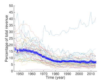
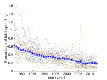
Using a coordinated crowd or swarm to solve complex problems is well studied in the literature. Particle swarm optimization (PSO) [3] is a widely adopted global optimization technique that uses a crowd of simple solvers to explore the fitness landscape of a problem. This swarm of PSO solvers mimics the swarming behavior observed in nature, e.g., among bees, ants, and birds. Each PSO solver revises its search direction based on its past performance and the position of the solver that observes the highest fitness. The PSO technique is very effective in solving deterministic problems that have multiple local extrema. However, PSO or any other parallel computing methodology cannot help us in improving the rate for learning in the optimal taxation and expenditure setting. The critical difference is that in the PSO setting each solver observes the same function; however, the reward or fitness of an individual in a crowd is typically subjective, private, very noisy, and often, not even numerically expressible. On the other hand, the inputs to the fitness function are numerically well defined. We exploit this feature to develop a learning algorithm.

Wisdom of crowds describes the phenomenon — first introduced as vox populi in 1907 by Francis Galton [4], then rediscovered and popularized by James Surowiecki a century later [5] — that the average opinion of a crowd is remarkably close to the otherwise unknown truth although the opinions of individuals in the crowd are very erroneous. This phenomenon partially justifies the efficiency of polling and prediction markets, where a surveyor can gather an accurate estimate of an unknown variable by averaging over multiple independent and informed guesses. Explanations [6, 7, 8] for the success of the wisdom of crowds assume that individuals’ estimates are unbiased and independently distributed [5, 9, 10, 11, 12, 13]. Social influence renders the wisdom of crowds ineffective  [10, 11, 14], and in order to guarantee accuracy, interactions among the respondents should be discouraged. Since individuals make decisions solely based on their prior knowledge and expertise, some even suggest vox expertorum, instead of vox populi, to be a more suitable name [10, 15, 16].

Increasingly, today individuals are getting all their information from highly inter-connected online social networks; thus, truly independent opinions are becoming rare. The existing literature suggests that vox populi should not be effective. And yet, online networks with very high degree of social interaction appear to be able to harness information effectively to benefit the individuals. We are relying on polling evermore, for selecting movies, restaurants, books, shows, etc. The polls appear to be working in identifying good options, even though the votes are highly correlated. The crowd benefits from these interactions by converging to optimum faster. Social influence here improves, rather than undermines, the collective learning process. How does one reconcile with the previous results on the degradation of the impact of vox populi in the presence of social influence? Is there an optimal degree of social influence for a learning crowd? This is the question we address in this study.

In this work, we use control theory to show that self-interested decision makers can benefit by partially following the wisdom of crowds. Too little social influence prevents individuals to harness the wisdom of crowds effect; however, too high a social influence has an adverse effect on the accuracy of the wisdom of crowds. The optimal degree of social influence balances these two effects.

We designed a human subject experiment called the “Fitness Game” that mimics the real-world situation where individuals alter their diets to improve health. By analyzing experiment results, we identify the individual learning dynamics, determine the average degree of social influence when subjects partially follow the wisdom of crowds feedback, and calculate the optimal degree of social influence that could have maximally improved the crowd’s performance.

II Experiment Design

We conducted an online experiment on Amazon Mechanical Turk with human subjects. There were three sets of experiments: B, N, and S. We focus our analysis on set B ($N=194$) only but present the final results for all three sets. Each set consisted of five replications of the experiment with its unique conditions.

The participants (or players of the “Fitness Game”) were asked to estimate the “diet level” that maximizes the “fitness” of a virtual character. The true relationship between the diet level and fitness was a given deterministic and concave function (i.e., there exists a unique diet level that maximizes the fitness); however, the players received a noisy value of the fitness associated with the guessed diet level. This noise, in reality, could be from other external factors such as environment and mood. The players were allowed multiple guesses, and were rewarded instantly based on the character’s fitness level. The players also received monetary rewards based on their relative performances.

We conducted five replications of the “Fitness Game” for each experiment set. In replication $p\in\{1,\ldots,5\}$, the $n_{p}$ participants first entered a session where they played the game in an open loop for 240 seconds (four minutes). In this session, each participant entered a series of guesses to best predict the unknown optimal diet level $\theta^{\ast}\in[2000,2500]$ kcal. When a player entered a guess for the optimal $\theta^{\ast}$, the interface would refresh and the player would see the virtual character’s fitness level (maximum $100$%) for the guessed value. The player could then enter a new value until this session ended. The term open loop indicates that individual decisions did not interact with each other; thus, the vox populi feedback was absent.

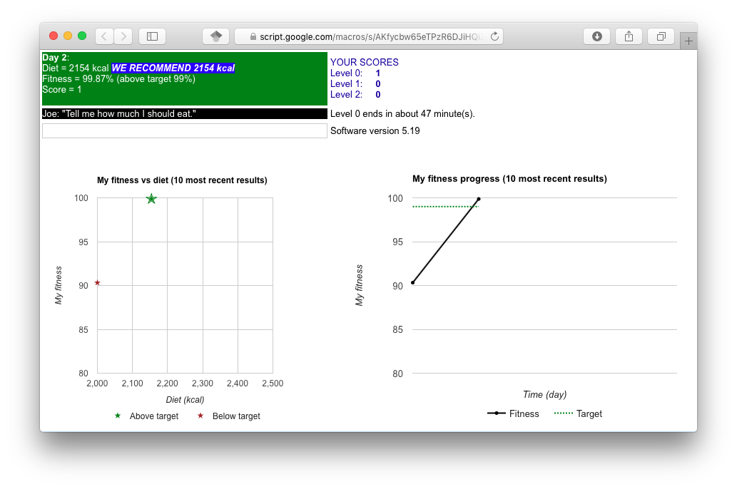
Subsequently, the same cohort entered the treatment session where they played the same game with a population feedback. The game was reset and a new optimal diet level $\theta^{\ast}$ was chosen. In this session, in addition to the fitness level corresponding to their own guess $z$, players also received a feedback saying “We recommend $\frac{1}{n_{p}}\sum_{i=1}^{n_{p}}{z}_{i}$ kcal,” where ${z}_{i}$ denotes the most recent guess of the $i$-th player. This feedback only updated when the players took actions. The players had the option of using the feedback in any manner they desired. See Appendix A for detailed descriptions of the “Fitness Game” interface.

In this treatment group, we revealed the population average of the diet level to each player. Thus, the choices of the players were not independent. However, we allowed the players the freedom to accept, reject, or partially accept such a population feedback, i.e., set the diet level to be a combination of their individual guesses and the feedback. We call this “soft feedback” in the sense that learners are allowed to choose the degree to which they adopt the feedback.

In a previous work [17], we had introduced the possibility of partial acceptance of population recommendation in the context of regulating emerging industries. In the regulatory context, we termed this as “soft” regulation in contrast to the conventional “hard” regulation where the regulated entities face fines and other punitive consequences for non-compliance. In our current setting, the individuals are allowed to partially accept the population feedback. This contrasts feedback in control theory, which is hard in the sense that it has to be followed. We showed that soft regulation is appropriate and efficient (and desirable) when the observed outcomes are very noisy, individual decision makers are rational utility-maximizing agents, and the agents are exploiting abundant resources, and therefore, not competing. Medical research and health optimization using large-scale social interactions, for example via Apple’s ResearchKit and CareKit [18], are examples of systems that satisfy these three conditions. The “Fitness Game” is meant to mimic these conditions.

Upon completion, participants received monetary rewards based on their relative game scores within the same cohort. We hoped to incentivize the participants in this way so that they would make rational decisions and actively optimize their virtual character’s fitness, instead of making random guesses to get the participation rewards.

III A Multi-Agent Control Model

We propose the following state-space control model to describe the collective dynamics of an $n$-agent crowd in the open loop setting:

$$x_{i}(t+1)=g_{i}\big{(}x_{i}(t)\big{)}+\omega_{i}(t).$$ (1)

In the soft feedback setting, we have

$$x_{i}(t+1) =(1-\beta_{i})\Big{(}g_{i}\big{(}x_{i}(t)\big{)}+{\omega}_{i}(t)\Big{)}+\beta_{i}u(t).$$ (2)

where $x_{i}(t)$ is the state variable of the $i$-th agent $(i=1,\ldots,n)$ at time $t$; $g_{i}(\cdot)$ is the learning function; $\omega_{i}(t)$ is a zero-mean random variable; $u(t)$ is the soft feedback, and $\beta_{i}$ is the degree of social influence.

III-A State $x_{i}(t)$ of the $i$-th Agent

The state variable $x_{i}(t)=z_{i}(t)-\theta^{\ast}$ is the decision error, i.e., difference between the individual decision $z_{i}(t)$ and the optimal decision $\theta^{\ast}$. $x_{i}^{*}=0$ indicates the optimal state (or the solution).

III-B Learning Function $g_{i}(\cdot)$ and Noise $\omega_{i}(t)$

The learning function $g_{i}$ of the $i$-th player encodes the process where the agent makes a decision, observes the corresponding utility, and then updates the state. We assume that the optimal state $x_{i}^{\ast}=0$ is an attracting and unique fixed point of $g_{i}(\cdot)$, i.e., $g_{i}(0)=0$. Thus, regardless of the optimization technique or the initial decision, an agent can always reach the optimum. We further assume that $g_{i}(x)$ is differential and $|g^{\prime}_{i}(x)|<1$, i.e., $g_{i}(x)$ is a contraction [19]. The closer $|g_{i}^{\prime}(x)|$ is to $1$, the slower $g_{i}(x)$ converges. From mean value theorem, we can also establish that $g_{i}(x)/x=g_{i}^{\prime}(\delta x)$, where $0\leq\delta\leq 1$, is strictly less than 1. We define learning gain, denoted by $\tilde{g}_{i}^{\prime}\equiv g_{i}(x)/x$, as the amplification of decision error.

$\omega_{i}(t)$ is a zero-mean random variable with variance $\sigma_{\omega}^{2}$ sampled at $t$. It represents the impact of the error in function evaluation on the decision. Such error can be a result of noise in measurement or external disturbance.

III-C Soft Feedback $u(t)$

We denote the soft feedback as the population average:

$$u(t)=\frac{1}{n}\sum_{j=1}^{n}x_{j}(t).$$ (3)

Again, unlike feedback in control theory, soft feedback does not have to be followed. The value of $u$ represents the error of the wisdom of crowds.

III-D Degree of Social Influence $\beta_{i}$

The degree of social influence denotes the weight the $i$-th player places on the feedback while learning. $\beta_{i}=0$ reduces the soft feedback setting in (2) to the open loop setting in (1).

III-E Convergence of the Soft Feedback Mechanism

We have previously established the following properties of soft feedback [17]: Social influence does not destabilize the system, nor does it alter the convergence provided $0\leq\beta_{i}<100\%$. We can write the noiseless soft feedback dynamics by replacing $g_{i}(\cdot)$ with the learning gain $\tilde{g}_{i}^{\prime}(t)$ computed at $t$:

$$x_{i}(t+1)=(1-\beta_{i})\tilde{g}_{i}^{\prime}(t)x_{i}(t)+\beta_{i}u(t).$$ (4)

In vector form, we have

$$\mathbf{x}(t+1)=(I-B)G^{\prime}(t)\mathbf{x}(t)+BS\mathbf{x}(t),$$ (5)

where $\mathbf{x}(t)=[x_{1}(t),\ldots,x_{n}(t)]^{\top}$, $B=\operatorname{diag}(\beta_{1},\ldots,\beta_{n})$, $G^{\prime}(t)=\operatorname{diag}\big{(}\tilde{g}_{1}^{\prime}(t),\ldots,\tilde{g}_{n}^{\prime}(t)\big{)}$, and $S=\frac{1}{n}\mathbf{1}\mathbf{1}^{\top}$. It is easy to identify that the largest eigenvalue of the matrix $(I-B)G^{\prime}(t)+BS$ is always strictly less than 1 if $0\leq\beta_{i}<100\%$. This implies the soft feedback dynamics also converges to the solution and is robust against bounded noise. See Appendix B for detailed proofs.

III-F Efficiency of the Soft Feedback Mechanism

We define the following optimal control problem for computing the optimal degree of social influence $\beta_{i}$ that minimizes the cost function $V$:

$$\min_{B}\quad V\big{(}B;\mathbf{x}(0),\boldsymbol{\omega}(t),T\big{)}=\mathbb{E}\left[\sum_{t=0}^{T-1}\frac{1}{n}\mathbf{x}(t)^{\top}\mathbf{x}(t)\right],$$ (6)

$$\operatorname{s.t.}\quad\mathbf{x}(t+1)=(I-B)\big{(}G^{\prime}(t)\mathbf{x}(t)+\boldsymbol{\omega}(t)\big{)}+BS\mathbf{x}(t),$$ (7)

where $\boldsymbol{\omega}(t)=[\omega_{1}(t),\ldots,\omega_{n}(t)]^{\top}$ denotes a series of noise vectors. The above optimal control problem minimizes the cumulative expected mean squared errors (MSE) over a finite time horizon $T$.

The time evolution of the total MSE in (6) depends on two factors: the rate of convergence controlled by $\big{(}(I-B)G^{\prime}(t)+BS\big{)}\mathbf{x}(t)$ and the noise reduction controlled by $(I-B)\boldsymbol{\omega}(t)$. A stronger social influence, i.e., high $\beta_{i}$, leads to less noise. The contraction effect depends on the largest singular value of the matrix $(I-B)G^{\prime}(t)+BS$. Given $G^{\prime}(t)$ and $S$, there always exists a social influence profile $B$ such that the largest singular value is minimized.

The overall problem is a non-convex optimization problem and difficult to solve analytically. We further simplify the problem by assuming $\tilde{g}^{\prime}_{i}(t)\equiv\tilde{g}$ is uniform across all participants, and the learning function is approximately linear. Similarly, we assume $\beta_{i}\equiv\beta$ is uniform across participants. The original dynamics is reduced into the following linear stochastic dynamics:

$$\mathbf{x}(t+1)=\big{[}(1-\beta)\tilde{g}+\beta S\big{]}\mathbf{x}(t)+(1-\beta)\boldsymbol{\omega}(t).$$ (8)

We can obtain the upper bound of the expected MSE as

$$\mathbb{E}\big{[}\operatorname{MSE}(t+1)\big{]}\leq m^{2}\operatorname{MSE}(t)+(1-\beta)^{2}\sigma_{\omega}^{2},$$ (9)

where $m=(1-\beta)\tilde{g}+\beta$ (see Appendix B for detailed derivation). This is a conservative (or worst case) estimation of the expected MSE evolution. The practice of computing the optimal control against worst case scenario is known as robust control. In this setting, one computes the control by minimizing the maximum cumulative expected MSE. We denote the robust solution as $\beta^{\ast}_{\text{R}}$:

$$\beta^{\ast}_{\text{R}}=\min_{\beta}\max_{\boldsymbol{\omega}(t)}V\big{(}\beta,\boldsymbol{\omega}(t);\mathbf{x}(0),T\big{)}.$$ (10)

The worst case $V(T)$ follows

$$\frac{V(T)}{\operatorname{MSE}(0)} \leq\left[\frac{1-m^{2T}}{1-m^{2}}+\right.$$ (11)

$$\left.\left(T-\frac{1-m^{2T}}{1-m^{2}}\right)\frac{(1-\beta)^{2}}{1-m^{2}}\frac{\sigma_{\omega}^{2}}{\operatorname{MSE}(0)}\right].$$

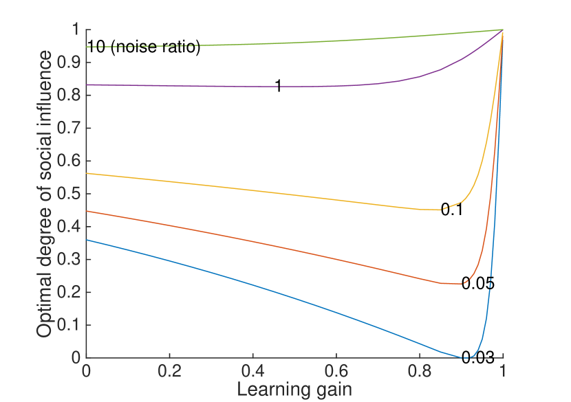
In Fig. 2 we plot the value of $\beta^{\ast}_{\text{R}}$ as a function of the noise-to-initial-MSE ratio $\sigma_{\omega}^{2}/\operatorname{MSE}(0)$ and the characteristic learning gain $\tilde{g}$ (given $T=30$ and $n=40$). A moderate social influence is optimal when systems are uncertain and one needs the system to equilibrate quickly.

Figure 2: Optimal degree of social influence from robust control by minimizing the RHS of (11). The general trend is that a moderately strong social influence is desirable if the system is uncertain (high noise-to-initial-MSE ratio) or the learning gain is low (fast open loop convergence). An interesting observation is that as the learning gain crosses a certain threshold (e.g., 0.9), the optimal degree of social influence rapidly increases as the learning gain increases. For a high learning gain, the contraction becomes insensitive to the change in $\beta$ while the noise reduction still does.

IV Results

IV-A Wisdom of Crowds Effect

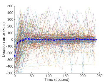
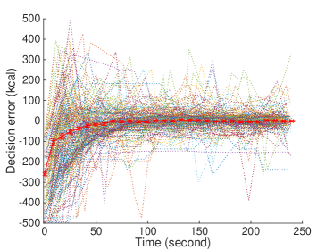
Let’s begin with the analysis of the wisdom of crowds effect. We plot the time series of each individual player’s decision error ($x_{i}$) as well as that of the wisdom of crowds ($u$) in Fig. 3 (similar to the state tax and expenditure time series in Fig. 1). The performance of the wisdom of crowds is clearly superior: $u$ steadily and quickly reaches the solution within the first minute while individual players lag behind.

Fig. 3 also confirms the behavior observed in the literature: The wisdom of crowds significantly outperforms the individual estimates, but such effect is weakened by social influence. The average in the soft feedback setting (red, right) slightly lags behind that in the open loop (blue, left).

Figure 3: Learning process of each individual player (time series of $x_{i}$) and the wisdom of crowds (time series of $u$) (left: open loop setting, right: soft feedback setting). Each colored dashed line represents an individual participant’s time series of decision error. The solid line is the arithmetic average of individual decision errors. Error bars reflect the standard errors of the mean.

IV-B Improvement from Soft Feedback

Now, let’s analyze how soft feedback improves the crowd’s learning performance. By visually inspecting Fig. 3, we observe the narrowing of individual error distribution in the soft feedback setting: There are fewer extreme errors than those in the open loop setting; most guesses are confined within $\pm 100$ kcal around optimum. In contrast, there are a significant number of players making completely off guesses ($\pm 500$ kcal) in the open loop (even towards the end of sessions).

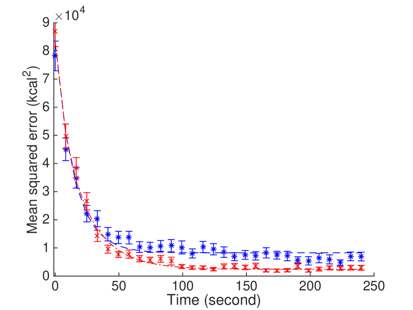
In Fig. 4 we plot the MSE time series to quantitatively assess the crowd’s performance. The total MSE is approximately $30$% lower in the soft feedback setting than in the open loop setting. Unlike the deterioration in the performance of wisdom of crowds, here social influence improves convergence and reduces the effect of noise. The critical feature of soft feedback is that the players can ignore the feedback. Since self-interested individuals reject feedbacks that appear unhelpful, the self-filtered social feedback significantly improves performance.

The observed improvement from soft feedback indicates that, without external interference, partially following the average opinion helped the players solve the “Fitness Game” problems. In the next section, we will characterize the system and estimate how much social influence was present in the experiment, and the optimal degree of social influence that would have optimized the crowd’s performance.

Figure 4: MSE progression. Blue (or red) dots are the MSE values sampled at different points in time ($T=30$) in the open loop (or soft feedback) setting. The dashed lines are simulation results based on models from system identification.

IV-C System Identification

We assumed that $g_{i}(x)\equiv g(x)=\tilde{g}x$ and the degree of social influence $\beta_{i}\equiv\beta$. The estimate $\hat{g}(x)=0.75x$ and $\hat{\sigma}_{\omega}=60$ ($r^{2}=0.97$) was computed using the open loop results. From (9), we first estimated $\tilde{g}$ and $\sigma_{\omega}$ by regressing $\operatorname{MSE}(t+1)$ against $\operatorname{MSE}(t)$. Using these estimates as an initial guess, we then ran a Monte Carlo simulation with 5000 samples and computed the average MSE time series. By minimizing the mean squared difference between that with the open loop MSE time series, we obtained the $\tilde{g}$ and $\sigma_{\omega}$ estimates. The corresponding MSE evolution is plotted in Fig. 4.

The estimate $\hat{\beta}=32\%$ ($r^{2}=0.99$) for the degree of social influence was computed using the results where the players received the population feedback. The corresponding MSE evolution is plotted in Fig. 4. Following the studies [20, 21] that have established that people rely more on themselves when the opinions of others are very dissimilar, we computed an “opinion distance” function $\beta(d)$, where $d=|g(x)-u|$ is the distance of an individual decision from the population feedback. We found it to be $\hat{\beta}(d)=\exp(-0.011d)$ ($r^{2}=0.98$).

IV-D Optimal Degree of Social Influence

Figure 5: Monte Carlo simulation of the expected MSE time series. Blue (or red) dashed line with $\ast$ (or $\times$) markers is the simulation of the open loop (or soft feedback) MSE. Left: Red dashed line is the simulation of the soft feedback MSE with estimate social influence profile $\hat{\beta}(d)$; magenta dotted line is the simulation of MSE with optimal degree of social influence $\beta^{\ast}_{\text{R}}$ through robust control; black dash-dot line is with true optimal degree of social influence $\beta^{\ast}_{\text{MC}}$; black solid line is with true optimal social influence profile $\beta^{\ast}_{\text{MC}}(d)$. Right: Red dashed line with markers is with dynamic social influence $\beta^{\ast}_{\text{R}}(t)$; magenta dotted line is the dynamic social influence time series.

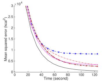
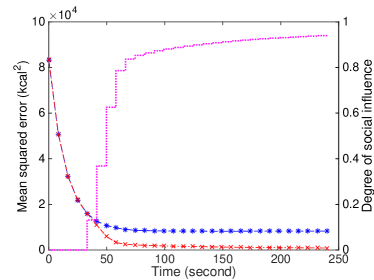
Given the estimates $\hat{g}(x)$ and $\hat{\sigma}_{\omega}$, one can compute the optimal degree of social influence $\beta^{\ast}$ that, hypothetically, would optimize the soft feedback performance. The results are summarized in Table I, and the associated MSE time series are displayed in Fig. 5. We first consider the case where the degree of social influence $\beta$ is fixed. The empirical estimate $\hat{\beta}$ of social influence computed from experiment data is listed as a reference. The robust social influence ${\beta}^{\ast}_{\text{R}}$ was calculated by minimizing the RHS in (11), i.e., optimizing the worst case cumulative expected MSE. The Monte Carlo (MC) estimate ${\beta}^{\ast}_{\text{MC}}$ was calculated by minimizing the total MSE in (6) with the expectation approximated by a Monte Carlo estimate. We regard $\beta^{\ast}_{\rm MC}$ as the true optimal degree of social influence. In Table I, the column labeled $\Delta$MSE lists the decrease of the cumulative expected MSE from the open loop to the soft feedback setting. The performances of the empirical estimate $\hat{\beta}$, the robust estimate $\beta^{\ast}_{\text{R}}$, and the optimal value $\beta^{\ast}_{\text{MC}}$ are quite close. It is comforting to know that the social influence present in the experiment was close to the optimum.

We expect the degree of social influence, a function of the opinion distance or a function of time, to likely improve convergence. The $\hat{\beta}(d)$ profile estimated from experimental data results in $\Delta\text{MSE}=30\%$, which is not distinguishable from the performance of a constant $\beta$. However, the optimal $\beta$ profile ${\beta}^{\ast}_{\text{MC}}(d)$ with $\Delta\text{MSE}=47\%$ is significantly superior. The performance of the optimal dynamic robust social influence $\beta^{\ast}_{\text{R}}(t)$ is also listed in Table I. Since we do not have evidence to suggest the subjects used a dynamic value for $\beta$, and the performance of $\hat{\beta}(d)$ is close to $\hat{\beta}$, we assume that the subjects used the constant $\hat{\beta}$ for the rest of our results.

TABLE I: Optimal degree of social influence

Type Value $\Delta$MSE $\beta$ (observed) $\hat{\beta}=32\%$ 29% $\beta$ (robust) $\beta^{\ast}_{\text{R}}=23\%$ 27% $\beta$ (MC, true optimum) $\beta^{\ast}_{\text{MC}}=30\%$ 29% $\beta$ profile (observed) $\hat{\beta}(d)=\exp(-0.011d)$ 30% $\beta$ profile (MC, true optimum) $\beta^{\ast}_{\text{MC}}(d)=\exp(-0.026d)$ 47% Dynamic $\beta$ (robust) $\beta^{\ast}_{\text{R}}(t)$ 39%

IV-E U.S. State Tax and Expenditure Case Study

Next, we apply this control-theoretic analysis to the state tax and expenditure case study. The results are displayed in Table II. The learning gains of the states are all very close to $1$, i.e., in a noiseless setting, the convergence is very slow. A possible explanation is that drastic change of tax and expenditure strategies is either prohibited or discouranged. A larger noise (see e.g., T09 and E065) or a smaller learning gain (see e.g., T20 and E65) calls for a larger optimal degree of social influence, which is consistent with the results presented in Fig. 2. The improvement from soft feedback ranges from $14$% to $73$%. As mentioned earlier, even a small improvement could make a significant difference in the nation’s overall welfare.

TABLE II: All Results

Description Duration Crowd size ($n$) Horizon ($T$) Learning gain ($\hat{\tilde{g}}$) Noise ($\hat{\sigma}_{\omega}$) $r^{2}$ Noise ratio Optimal $\beta$ $\Delta$MSE The Fitness Game (Set B) 0-240s 39 30 0.75 60 0.97 5% 30% 29% The Fitness Game (Set N) 0-240s 41 30 0.7 57 0.98 4% 32% 25% The Fitness Game (Set S) 0-240s 9 30 0.65 51 0.98 3% 30% 17% Total Gen Sales Tax (T09) 1946-2014 50 69 0.96 4 0.89 3% 35% 73% Total License Taxes (C118) 1946-2014 50 69 0.97 0.82 0.89 0.4% 14% 34% Alcoholic Beverage Lic (T20) 1946-2014 50 69 0.93 0.04 0.99 0.09% 20% 34% Individual Income Tax (T40) 1946-2014 50 69 0.98 2.9 0.86 1% 14% 32% Educ-NEC-Dir Expend (E037) 1977-2013 51 37 0.96 0.097 0.85 1% 28% 54% Emp Sec Adm-Direct Exp (E040) 1977-2013 51 37 0.93 0.037 0.99 0.6% 11% 14% Total Highways-Dir Exp (E065) 1977-2013 51 37 0.93 0.76 0.89 3% 31% 53% Liquor Stores-Tot Exp (E107) 1977-2013 51 37 0.95 0.17 0.95 1% 42% 67%

V Discussion

There is a fundamental difference between vox populi and the soft feedback mechanism proposed in this paper. Even though both come under the umbrella of “collective intelligence,” the vox populi aggregates the wisdom of experts while the latter harnesses the wisdom of learners. Experts base their opinions on prior knowledge. Such knowledge comes from experience and beliefs, which are unlikely to change. Independency and diversity of opinions prevent the “groupthink” behavior — undesirable convergence of individual estimates [22]. In this setting, social influence, which violates independency, reduces the accuracy of the wisdom of crowds.

Learners, on the other hand, revise their decisions by interacting with the problem as well as other learners. Consider, for example, flocking birds. The birds have to adapt to changing weather; they gather local information, follow their closest neighbors, and revise directions constantly [23]. In this collective learning environment, individuals, like the flocking birds, are both respondents who generate new information, and surveyors who poll their social networks to improve decisions.

It appears that a social influence degree of $30$% is robust across many different scenarios. In Table II, the optimal degree of social influence ranges from 30% to 32% for the “Fitness Game” experiment. Prior literature [20, 24, 25, 26, 27] also reports 30% to be the commonly observed degree of social influence on average. Whether this value is a mere coincidence requires further investigation.

The self-interested filtering of the feedback is key to ensuring the accuracy and efficiency of the soft feedback mechanism. Individuals will reject the feedbacks that appear useless. The experimentally observed magnitude of soft feedback is close to the theoretically predicted value for the optimal degree of social influence. This discovery suggests the promise of soft feedback for challenging real-world problems that require collective learning and action.

Appendix A The “Fitness Game”

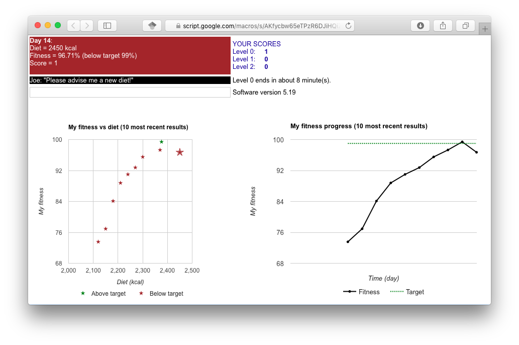
All experiments have been approved by the IRB of Columbia University (Protocol Number: IRB-AAAQ2603). We developed the “Fitness Game” using Google Apps Script and conducted the experiments on Amazon Mechanical Turk (AMT). All the data were stored in Google Sheets. Once the players accepted the task on AMT, they were first asked to carefully read the game instructions (see Fig. 6). The total task duration was ten minutes. The open loop (game level 1) and soft feedback (game level 2) sessions lasted precisely four minutes each. Players who wished to practice could enter the practice mode (game level 0) any time before open loop session began. After completing both open loop and soft feedback sessions, the players received a message about compensation information.

The interactive app (see Fig. 7) consists of the following components: The upper left panel shows the number of attempted guesses, the most recent guess, the fitness level, and the latest score. The panel changes from red to green whenever the player earns one point. In the soft feedback session, an additional message recommends the current vox populi population feedback (see Fig. 7, right). The upper right panel records latest game scores. The lower left scatter chart plots the ten most recent entries (fitness versus diet). The lower right line chart plots the fitness history of the ten most recent entries.

Figure 6: Instructions.

Figure 7: Game interface.

The virtual character’s random fitness level $f(x)$ as a function of the input $x=z-\theta^{\ast}$ was given by

$$f(x)=f_{0}-\Big{(}\frac{x}{\kappa}\Big{)}^{2}+\tilde{\omega},$$

where $f_{0}=98\%$ is the maximum achievable fitness, $\kappa=500~{}\text{kcal}$ is the scale of the fitness function, and $\tilde{\omega}$ is a sample from a random variable uniformly distributed over $[-2\%,2\%]$. The player was awarded one score point whenever the guess led to a fitness level of 99% or higher.

Appendix B Mathematical Model and Proofs

We first begin with the noiseless dynamics and then extend the model to include noise. The noiseless dynamics for the $n$-player “Fitness Game” is as follows:

$$x_{i}(t+1)=(1-\beta_{i})g_{i}\big{(}x_{i}(t)\big{)}+\beta_{i}u(t),$$

where $x_{i}(t)$ is the $i$-th player’s state, i.e., deviation from optimum $\theta^{\ast}$ at time $t$, and restricted to belong to a bounded set $\mathbb{X}\subseteq\mathbb{R}$, the learning function $g_{i}(\cdot)$ denotes the player’s own state update process, $\beta_{i}\in[0,1]$ (degree of social influence) is the weight player $i$ puts on the soft feedback $u(t)=\frac{1}{n}\sum_{i}x_{i}(t)$. Note that in the paper, we refer to $\beta$ as percentage. The individual learning functions $\{g_{i}(x):1\leq i\leq n\}$ are assumed to satisfy the following regularity condition:

Assumption 1.

For all $i\in\{1,\ldots,n\}$, the function $g_{i}$ is differentiable, $x^{\ast}=0$ is the unique attracting fixed point of $g_{i}$, and furthermore, $g_{i}$ is a contraction, i.e., $|g_{i}^{\prime}(x)|<1$ for all $1\leq i\leq n$ and $x\in\mathbb{X}$.

This assumption is motivated by the fact that all players converged to the optimal point in the open loop setting independent of the starting guess.

Let $\mathbf{x}\equiv[x_{1},\dots,x_{n}]^{\top}\in\mathbb{X}^{n}$ denote the state vector for the $n$ agents. The soft feedback map for the vector $\mathbf{x}$ is given by $\mathbf{x}(t+1)=\mathbf{h}\big{(}\mathbf{x}(t)\big{)}$ where the map

$$\mathbf{h}(\mathbf{x}) = \begin{bmatrix}(1-\beta_{1})g_{1}(x_{1})&\dots&0\\ \vdots&\ddots&\vdots\\ 0&\dots&(1-\beta_{n})g_{n}(x_{n})\end{bmatrix}+$$

$$\frac{1}{n}\begin{bmatrix}\beta_{1}\\ \vdots\\ \beta_{n}\end{bmatrix}\mathbf{1}^{\top}\mathbf{x}.$$

We first show that the state vector $\mathbf{x}(t)$ converges to $\mathbf{x}^{\ast}=\mathbf{0}$ if the functions $\{g_{i}(x):1\leq i\leq n\}$ satisfy Assumption 1 and $0\leq\max_{i}\beta_{i}<1$.

Theorem 1.

The spectral radius $\rho\big{(}J(\mathbf{x})\big{)}$ of the Jacobian matrix of the soft feedback map $\mathbf{h}(\mathbf{x})$ satisfies $\rho\big{(}J(\mathbf{x})\big{)}\leq m=\max_{1\leq i\leq n,x\in\mathbb{X}}\Big{\{}(1-\beta_{i})|g_{i}^{\prime}(x)|+\beta_{i}\Big{\}}<1$.

Proof.

The Jacobian of $\mathbf{h}(\mathbf{x})$ is

$$J(\mathbf{x}) = \operatorname{diag}\big{(}(1-\beta_{1})g_{1}^{\prime}(x_{1}),\dots,(1-\beta_{n})g_{n}^{\prime}(x_{n})\big{)}+$$

$$\frac{1}{n}\begin{bmatrix}\beta_{1}\\ \vdots\\ \beta_{n}\end{bmatrix}\mathbf{1}^{\top}.$$

The induced $\infty$-norm $\|J(\mathbf{x})\|_{\infty}$ of the Jacobian $J$ satisfies

$$\|J(\mathbf{x})\|_{\infty} = \max_{\|\mathbf{v}\|_{\infty}=1}\|J(\mathbf{x})\mathbf{v}\|_{\infty},$$

$$= \max_{\|\mathbf{v}\|_{\infty}=1}\max_{1\leq i\leq n}|J_{i}(\mathbf{x})\mathbf{v}|,$$

$$= \max_{\|\mathbf{v}\|_{\infty}=1}\max_{1\leq i\leq n}\Big{[}(1-\beta_{i})|g_{i}^{\prime}(x_{i})|v_{i}+$$

$$\frac{1}{n}\beta_{i}(\mathbf{1}^{\top}\mathbf{v})\Big{]},$$

$$\leq m(\mathbf{x}),$$

where $J_{i}(\mathbf{x})$ denotes the $i$-th row of the Jacobian $J(\mathbf{x})$. The result follows from noting that $\rho\big{(}J(\mathbf{x})\big{)}\leq\|J(\mathbf{x})\|_{\infty}=m(\mathbf{x})$. It is easy to see that $m(\mathbf{x})<1$ whenever $\max_{i}\beta_{i}<1$. ∎

This result immediately implies that $\mathbf{x}^{\ast}=0$ is an asymptotically stable fixed point of the map $\mathbf{h}(\mathbf{x})$.

Theorem 2.

The fixed point $\mathbf{x}^{\ast}=\mathbf{0}$ of the map $\mathbf{h}$ is robust when subjected to bounded disturbances.

Proof.

Let $V(\mathbf{x})=\|\mathbf{x}\|_{\infty}$. Since $\mathbf{h}(\mathbf{0})=\mathbf{0}$, the mean value theorem implies that

$$\mathbf{h}(\mathbf{x})=\begin{bmatrix}J_{1}(\delta_{1}\mathbf{x})\\ \vdots\\ J_{n}(\delta_{n}\mathbf{x})\end{bmatrix}\mathbf{x},$$

for some $\delta_{i}\in[0,1]$, $i=1,\ldots,n$, and $J_{i}(\delta_{i}\mathbf{x})$ denotes the $i$-th row of the Jacobian of $\mathbf{h}(\delta_{i}\mathbf{x})$. Thus,

$$V\big{(}\mathbf{h}(\mathbf{x})\big{)} =\|\mathbf{h}(\mathbf{x})\|_{\infty},$$

$$=\max_{1\leq i\leq n}|J_{i}(\delta_{i}\mathbf{x})\mathbf{x}|,$$

$$\leq\Big{(}\max_{1\leq i\leq n}\|J(\delta_{i}\mathbf{x})\|_{\infty}\Big{)}\|\mathbf{x}\|_{\infty},$$

$$<m\|\mathbf{x}\|_{\infty},$$

where the first inequality follows from the definition of $\|J(\delta_{i}\mathbf{x})\|_{\infty}$.

Since the continuous function $V(\mathbf{x})$ is a Lyapunov function for $\mathbf{h}$, the result follows from standard results in stability theory [28]. ∎

In the rest of this section, we will assume that $\beta_{i}$ are identically equal to $\beta$.

Theorem 3.

Suppose $\beta_{i}$ are all identically equal to $\beta$. Then $\|\mathbf{h}(\mathbf{x})\|_{2}\leq m\|\mathbf{x}\|_{2}$, where $m=(1-\beta)\max_{1\leq i\leq n,x\in\mathbb{X}}|g_{i}^{\prime}(x)|+\beta$.

Proof.

Using the mean value theorem, one can write

$$\mathbf{h}(\mathbf{x})=\Big{(}(1-\beta)\text{diag}\big{(}g_{1}^{\prime}(\delta_{1}x_{1}),\dots,g_{n}^{\prime}(\delta_{n}x_{n})\big{)}+\frac{\beta}{n}\mathbf{1}\mathbf{1}^{\top}\Big{)}\mathbf{x},$$

where $\delta_{i}\in[0,1]$ for $i=1,\ldots,n$. Let $G^{\prime}=\text{diag}(g_{1}^{\prime}(\delta_{1}x_{1}),\dots,g_{n}^{\prime}(\delta_{n}x_{n}))$ and $J=(1-\beta)G^{\prime}+\frac{\beta}{n}\mathbf{1}\mathbf{1}^{\top}$. Then

$$\|G^{\prime}\|_{2}^{2} = \max_{\|\mathbf{v}\|_{2}=1}\|G^{\prime}\mathbf{v}\|_{2}^{2},$$

$$= \max_{\|\mathbf{v}\|_{2}=1}\sum_{i}|g^{\prime}_{i}(\delta_{i}x)|^{2}v_{i}^{2},$$

$$\leq \max_{1\leq i\leq n}|g^{\prime}_{i}(\delta_{i}x_{i})|^{2}$$

$$\leq \max_{1\leq i\leq n,x\in\mathbb{X}}|g_{i}^{\prime}(x)|^{2}.$$

Thus, $\|G^{\prime}\|_{2}\leq\max_{1\leq i\leq n,x\in\mathbb{X}}|g_{i}^{\prime}(x)|$. Therefore,

$$\|J\|_{2}^{2} = \max_{\|\mathbf{v}\|_{2}=1}\|J\mathbf{v}\|_{2}^{2},$$

$$= \max_{\|\mathbf{v}\|_{2}=1}\left\{(1-\beta)^{2}\|G^{\prime}\mathbf{v}\|_{2}^{2}+\frac{\beta^{2}}{n^{2}}(\mathbf{1}^{\top}\mathbf{v})^{2}\|\mathbf{1}\|_{2}^{2}+\right.$$

$$\left.\frac{2\beta(1-\beta)}{n}(\mathbf{1}^{\top}\mathbf{v})(\mathbf{1}^{\top}G^{\prime}\mathbf{v})\right\},$$

$$\leq (1-\beta)^{2}\|G^{\prime}\|_{2}^{2}+\beta^{2}+$$

$$\frac{2\beta(1-\beta)}{n}\big{(}\max_{\|\mathbf{v}\|_{2}=1}|\mathbf{1}^{\top}v|\big{)}\big{(}\max_{\|\mathbf{v}\|_{2}=1}|\mathbf{1}^{\top}G^{\prime}\mathbf{v}|\big{)},$$

$$\leq (1-\beta)^{2}\|G^{\prime}\|_{2}^{2}+\beta^{2}+$$

$$\frac{2\beta(1-\beta)}{\sqrt{n}}\|\mathbf{1}\|_{2}\big{(}\max_{\|\mathbf{v}\|_{2}=1}\|G^{\prime}\mathbf{v}\|_{2}\big{)},$$

$$= (1-\beta)^{2}\|G^{\prime}\|_{2}^{2}+\beta^{2}+2\beta(1-\beta)\|G^{\prime}\|_{2}=m^{2}.$$

Since $\mathbf{h}(\mathbf{x})=J\mathbf{x}$, it follows that $\|\mathbf{h}(\mathbf{x})\|_{2}=\|J\mathbf{x}\|_{2}\leq\|J\|_{2}\|\mathbf{x}\|_{2}\leq m\|x\|_{2}$. ∎

Next, we introduce noise in the game dynamics. Let $\{\boldsymbol{\omega}(t)\in\mathbb{R}^{n}:t\geq 0\}$ denote an IID sequence of random vectors where $\boldsymbol{\omega}(t)=[\omega_{1}(t),\dots,\omega_{n}(t)]^{\top}$, and each $\omega_{i}(t)$ is an IID sample of a zero mean random variable with variance $\sigma_{\omega}^{2}$. The noisy game dynamics is given by

$$x_{i}(t+1)=(1-\beta_{i})\Big{(}g_{i}\big{(}x_{i}(t)\big{)}+\omega_{i}(t)\Big{)}+\beta_{i}u(t),$$

i.e., we replace $g_{i}\big{(}x_{i}(t)\big{)}$ by the noisy state update $g_{i}\big{(}x_{i}(t)\big{)}+\omega_{i}(t)$. This modification models the fact that the players sample a noisy version of the fitness function, and use these noisy samples to generate the update; therefore, we expect the state update to be noisy. Note that the noise is not measurement noise, rather noise in the function evaluation.

Define the mean squared error MSE

$$\operatorname{MSE}(t)=\frac{1}{n}\sum_{i}x_{i}(t)^{2}=\frac{1}{n}\|\mathbf{x}(t)\|_{2}^{2}.$$

Then

$$\mathbb{E}\big{[}\operatorname{MSE}(t+1)\mid\mathbf{x}(t)\big{]}$$ (12)

$$= \frac{1}{n}\mathbb{E}\Big{[}\|\mathbf{x}(t+1)\|_{2}^{2}\mid\mathbf{x}(t)\Big{]},$$

$$= \frac{1}{n}\mathbb{E}\Big{[}\|\mathbf{h}(\mathbf{x}(t))+(1-\beta)\boldsymbol{\omega}(t)\|_{2}^{2}\mid\mathbf{x}(t)\Big{]},$$

$$= \frac{1}{n}\|\mathbf{h}(\mathbf{x}(t))\|_{2}^{2}+\frac{(1-\beta)^{2}}{n}\mathbb{E}\big{[}\|\boldsymbol{\omega}(t)\|_{2}^{2}\big{]},$$

$$\leq \frac{m^{2}}{n}\|\mathbf{x}(t)\|_{2}^{2}+(1-\beta)^{2}\sigma_{\omega}^{2},$$ (13)

$$= m^{2}\operatorname{MSE}(t)+(1-\beta)^{2}\sigma_{\omega}^{2},$$ (14)

where (12) follows from the fact that $\boldsymbol{\omega}(t)$ is independent of $\mathbf{x}(t)$, and (13) follows from the bound in Theorem 3. Iterating the bound (14) we get

$$\mathbb{E}[\text{MSE}(t)]\leq m^{2t}\text{MSE}(0)+\frac{(1-\beta)^{2}(1-m^{2t})}{(1-m^{2})}\sigma_{\omega}^{2}.$$

References

- [1] T. U. C. Bureau, “Historical data,” State Government Tax Collection, 2015. [Online]. Available: https://www.census.gov/govs/statetax/historical_data.html
- [2] T. P. Center. (2015) Expenditure data for the united states (1977-2012). [Online]. Available: http://slfdqs.taxpolicycenter.org
- [3] J. Kennedy, “Particle swarm optimization,” in Encyclopedia of Machine Learning. Springer, 2010, pp. 760–766.
- [4] F. Galton, “Vox populi (the wisdom of crowds),” Nature, vol. 75, pp. 450–451, 1907.
- [5] J. Surowiecki, The wisdom of crowds. Anchor, 2005.
- [6] N. De Condorcet, Essai sur l’application de l’analyse à la probabilité des décisions rendues à la pluralité des voix. Cambridge University Press, 2014.
- [7] G. Bergman and K. O. Donner, An analysis of the spring migration of the common scoter and the long-tailed duck in southern Finland. Societas pro fauna et flora Fennica, 1964.
- [8] A. M. Simons, “Many wrongs: the advantage of group navigation,” Trends in ecology & evolution, vol. 19, no. 9, pp. 453–455, 2004.
- [9] A. Kittur and R. E. Kraut, “Harnessing the wisdom of crowds in wikipedia: quality through coordination,” in Proceedings of the 2008 ACM conference on Computer supported cooperative work. ACM, 2008, pp. 37–46.
- [10] R. L. Goldstone and T. M. Gureckis, “Collective behavior,” Topics in cognitive science, vol. 1, no. 3, pp. 412–438, 2009.
- [11] J. Lorenz, H. Rauhut, F. Schweitzer, and D. Helbing, “How social influence can undermine the wisdom of crowd effect,” Proceedings of the National Academy of Sciences, vol. 108, no. 22, pp. 9020–9025, 2011.
- [12] A. J. Quinn and B. B. Bederson, “Human computation: a survey and taxonomy of a growing field,” in Proceedings of the SIGCHI conference on human factors in computing systems. ACM, 2011, pp. 1403–1412.
- [13] G. A. Alvarez, “Representing multiple objects as an ensemble enhances visual cognition,” Trends in cognitive sciences, vol. 15, no. 3, pp. 122–131, 2011.
- [14] D. J. Sumpter and S. C. Pratt, “Quorum responses and consensus decision making,” Philosophical Transactions of the Royal Society of London B: Biological Sciences, vol. 364, no. 1518, pp. 743–753, 2009.
- [15] F. Galton, “The ballot-box,” Nature, vol. 75, pp. 509–510, 1907.
- [16] L. Conradt and T. J. Roper, “Consensus decision making in animals,” Trends in ecology & evolution, vol. 20, no. 8, pp. 449–456, 2005.
- [17] Y. Luo, G. Iyengar, and V. Venkatasubramanian, “Soft regulation with crowd recommendation: Coordinating self-interested agents in sociotechnical systems under imperfect information,” PLoS ONE, vol. 11, no. 3, p. e0150343, 2016.
- [18] Apple. (2016) Researchkit and carekit. [Online]. Available: http://www.apple.com/researchkit/
- [19] F. E. Browder, “Fixed-point theorems for noncompact mappings in hilbert space,” Proceedings of the National Academy of Sciences, vol. 53, no. 6, pp. 1272–1276, 1965.
- [20] J. B. Soll and R. P. Larrick, “Strategies for revising judgment: How (and how well) people use others’ opinions.” Journal of Experimental Psychology: Learning, Memory, and Cognition, vol. 35, no. 3, p. 780, 2009.
- [21] M. Moussaïd, J. E. Kämmer, P. P. Analytis, and H. Neth, “Social influence and the collective dynamics of opinion formation,” PLoS One, vol. 8, no. 11, p. e78433, 2013.
- [22] C. Sunstein and R. Hastie, Wiser: Getting Beyond Groupthink to Make Groups Smarter. Harvard Business Review Press, 2014.
- [23] C. W. Reynolds, “Flocks, herds and schools: A distributed behavioral model,” in Proceedings of the 14th annual conference on Computer graphics and interactive techniques, ser. SIGGRAPH ’87. New York, NY, USA: ACM, 1987, pp. 25–34.
- [24] N. Harvey and I. Fischer, “Taking advice: Accepting help, improving judgment, and sharing responsibility,” Organizational Behavior and Human Decision Processes, vol. 70, no. 2, pp. 117–133, 1997.
- [25] J. S. Lim and M. O’Connor, “Judgemental adjustment of initial forecasts: Its effectiveness and biases,” Journal of Behavioral Decision Making, vol. 8, no. 3, pp. 149–168, 1995.
- [26] I. Yaniv, “Receiving other people’s advice: Influence and benefit,” Organizational Behavior and Human Decision Processes, vol. 93, no. 1, pp. 1–13, 2004.
- [27] I. Yaniv and E. Kleinberger, “Advice taking in decision making: Egocentric discounting and reputation formation,” Organizational behavior and human decision processes, vol. 83, no. 2, pp. 260–281, 2000.
- [28] A. R. Teel, “Discrete time receding horizon optimal control: Is the stability robust?” in Optimal Control, Stabilization and Nonsmooth Analysis. Springer, 2004, pp. 3–27.