Topology and Geometry of Half-Rectified Network Optimization
Abstract
The loss surface of deep neural networks has recently attracted interest in the optimization and machine learning communities as a prime example of high-dimensional non-convex problem. Some insights were recently gained using spin glass models and mean-field approximations, but at the expense of strongly simplifying the nonlinear nature of the model.
In this work, we do not make any such assumption and study conditions on the data distribution and model architecture that prevent the existence of bad local minima. Our theoretical work quantifies and formalizes two important folklore facts: (i) the landscape of deep linear networks has a radically different topology from that of deep half-rectified ones, and (ii) that the energy landscape in the non-linear case is fundamentally controlled by the interplay between the smoothness of the data distribution and model over-parametrization. Our main theoretical contribution is to prove that half-rectified single layer networks are asymptotically connected, and we provide explicit bounds that reveal the aforementioned interplay.
The conditioning of gradient descent is the next challenge we address. We study this question through the geometry of the level sets, and we introduce an algorithm to efficiently estimate the regularity of such sets on large-scale networks. Our empirical results show that these level sets remain connected throughout all the learning phase, suggesting a near convex behavior, but they become exponentially more curvy as the energy level decays, in accordance to what is observed in practice with very low curvature attractors.
1 Introduction
Optimization is a critical component in deep learning, governing its success in different areas of computer vision, speech processing and natural language processing. The prevalent optimization strategy is Stochastic Gradient Descent, invented by Robbins and Munro in the 50s. The empirical performance of SGD on these models is better than one could expect in generic, arbitrary non-convex loss surfaces, often aided by modifications yielding significant speedups Duchi et al. , (2011); Hinton et al. , (2012); Ioffe & Szegedy, (2015); Kingma & Ba, (2014). This raises a number of theoretical questions as to why neural network optimization does not suffer in practice from poor local minima.
The loss surface of deep neural networks has recently attracted interest in the optimization and machine learning communities as a paradigmatic example of a hard, high-dimensional, non-convex problem. Recent work has explored models from statistical physics such as spin glasses Choromanska et al. , (2015), in order to understand the macroscopic properties of the system, but at the expense of strongly simplifying the nonlinear nature of the model. Other authors have advocated that the real danger in high-dimensional setups are saddle points rather than poor local minima Dauphin et al. , (2014), although recent results rigorously establish that gradient descent does not get stuck on saddle points Lee et al. , (2016) but merely slowed down. Other notable recent contributions are Kawaguchi, (2016), which further develops the spin-glass connection from Choromanska et al. , (2015) and resolves the linear case by showing that no poor local minima exist; Sagun et al. , (2014) which also discusses the impact of stochastic vs plain gradient, Soudry & Carmon, (2016), that studies Empirical Risk Minimization for piecewise multilayer neural networks under overparametrization (which needs to grow with the amount of available data), and Goodfellow et al. , (2014), which provided insightful intuitions on the loss surface of large deep learning models and partly motivated our work. Additionally, the work Safran & Shamir, (2015) studies some topological properties of homogeneous nonlinear networks and shows how overparametrization acts upon these properties, and the pioneering Shamir, (2016) studied the distribution-specific hardness of optimizing non-convex objectives. Lastly, several papers submitted concurrently and independently of this one deserve note, particularly Swirszcz et al. , (2016) which analyzes the explicit criteria under which sigmoid-based neural networks become trapped by poor local minima, as well as Tian, (2017), which offers a complementary study of two layer ReLU based networks, and their learning dynamics.
In this work, we do not make any linearity assumption and study conditions on the data distribution and model architecture that prevent the existence of bad local minima. The loss surface of a given model can be expressed in terms of its level sets , which contain for each energy level all parameters yielding a loss smaller or equal than . A first question we address concerns the topology of these level sets, i.e. under which conditions they are connected. Connected level sets imply that one can always find a descent direction at each energy level, and therefore that no poor local minima can exist. In absence of nonlinearities, deep (linear) networks have connected level sets Kawaguchi, (2016). We first generalize this result to include ridge regression (in the two layer case) and provide an alternative, more direct proof of the general case. We then move to the half-rectified case and show that the topology is intrinsically different and clearly dependent on the interplay between data distribution and model architecture. Our main theoretical contribution is to prove that half-rectified single layer networks are asymptotically connected, and we provide explicit bounds that reveal the aforementioned interplay.
Beyond the question of whether the loss contains poor local minima or not, the immediate follow-up question that determines the convergence of algorithms in practice is the local conditioning of the loss surface. It is thus related not to the topology but to the shape or geometry of the level sets. As the energy level decays, one expects the level sets to exhibit more complex irregular structures, which correspond to regions where has small curvature. In order to verify this intuition, we introduce an efficient algorithm to estimate the geometric regularity of these level sets by approximating geodesics of each level set starting at two random boundary points. Our algorithm uses dynamic programming and can be efficiently deployed to study mid-scale CNN architectures on MNIST, CIFAR-10 and RNN models on Penn Treebank next word prediction. Our empirical results show that these models have a nearly convex behavior up until their lowest test errors, with a single connected component that becomes more elongated as the energy decays. The rest of the paper is structured as follows. Section 2 presents our theoretical results on the topological connectedness of multilayer networks. Section 3 presents our path discovery algorithm and Section 4 covers the numerical experiments.
2 Topology of Level Sets
Let be a probability measure on a product space , where we assume and are Euclidean vector spaces for simplicity. Let be an iid sample of size drawn from defining the training set. We consider the classic empirical risk minimization of the form
| (1) |
where encapsulates the feature representation that uses parameters and is a regularization term. In a deep neural network, contains the weights and biases used in all layers. For convenience, in our analysis we will also use the oracle risk minimization:
| (2) |
Our setup considers the case where consists on either or norms, as we shall describe below. They correspond to well-known sparse and ridge regularization respectively.
2.1 Poor local minima characterization from topological connectedness
We define the level set of as
| (3) |
The first question we study is the structure of critical points of and when is a multilayer neural network. For simplicity, we consider first a strict notion of local minima: is a strict local minima of if there is with for all and . In particular, we are interested to know whether has local minima which are not global minima. This question is answered by knowing whether is connected at each energy level :
Proposition 2.1.
If is connected for all then every local minima of is a global minima.
Strict local minima implies that and , but avoids degenerate cases where is constant along a manifold intersecting . In that scenario, if denotes that manifold, our reasoning immediately implies that if are connected, then for all there exists with and . In other words, some element at the boundary of must be a saddle point. A stronger property that eliminates the risk of gradient descent getting stuck at is that all elements at the boundary of are saddle points. This can be guaranteed if one can show that there exists a path connecting any to the lowest energy level such that is strictly decreasing along it.
Such degenerate cases arise in deep linear networks in absence of regularization. If denotes any parameter value, with denoting the hidden layer sizes, and are arbitrary elements of the general linear group of invertible matrices with positive determinant, then
In particular, has a Lie Group structure. In the half-rectified nonlinear case, the general linear group is replaced by the Lie group of homogeneous invertible matrices with .
This proposition shows that a sufficient condition to prevent the existence of poor local minima is having connected level sets, but this condition is not necessary: one can have isolated local minima lying at the same energy level. This can be the case in systems that are defined up to a discrete symmetry group, such as multilayer neural networks. However, as we shall see next, this case puts the system in a brittle position, since one needs to be able to account for all the local minima (and there can be exponentially many of them as the parameter dimensionality increases) and verify that their energy is indeed equal.
2.2 The Linear Case
We first consider the particularly simple case where is a multilayer network defined by
| (4) |
and the ridge regression . This model defines a non-convex (and non-concave) loss . When , it has been shown in Saxe et al. , (2013) and Kawaguchi, (2016) that in this case, every local minima is a global minima. We provide here an alternative proof of that result that uses a somewhat simpler argument and allows for in the case .
Proposition 2.2.
Let be weight matrices of sizes , , and let , denote the risk minimizations using as in (4). Assume that for . Then (and ) is connected for all and all when , and for when ; and therefore there are no poor local minima in these cases. Moreover, any can be connected to the lowest energy level with a strictly decreasing path.
Let us highlight that this result is slightly complementary than that of Kawaguchi, (2016), Theorem 2.3. Whereas we require for and our analysis does not inform about the order of the saddle points, we do not need full rank assumptions on nor the weights .
This result does also highlight a certain mismatch between the picture of having no poor local minima and generalization error. Incorporating regularization drastically changes the topology, and the fact that we are able to show connectedness only in the two-layer case with ridge regression is profound; we conjecture that extending it to deeper models requires a different regularization, perhaps using more general atomic norms Bach, (2013). But we now move our interest to the nonlinear case, which is more relevant to our purposes.
2.3 Half-Rectified Nonlinear Case
We now study the setting given by
| (5) |
where . The biases can be implemented by replacing the input vector with and by rebranding each parameter matrix as
where contains the biases for each layer. For simplicity, we continue to use and in the following.
2.3.1 Nonlinear models are generally disconnected
One may wonder whether the same phenomena of global connectedness also holds in the half-rectified case. A simple motivating counterexample shows that this is not the case in general. Consider a simple setup with drawn from a mixture of two Gaussians and , and let , where is the (hidden) mixture component taking values. Let be a single-hidden layer ReLU network, with two hidden units. Let be a configuration that bisects the two mixture components, and let the same configuration, but swapping the bisectrices. One can verify that they can both achieve arbitrarily small risk by letting the covariance of the mixture components go to . However, any path that connects to must necessarily pass through a point in which has rank , which leads to an estimator with risk at least .
In fact, it is easy to see that this counter-example can be extended to any generic half-rectified architecture, if one is allowed to adversarially design a data distribution. For any given with arbitrary architecture and current parameters , let be the underlying tessellation of the input space given by our current choice of parameters; that is, is piece-wise linear and contains those pieces. Now let be any arbitrary distribution with density for all , for example a Gaussian, and let . Since is invariant under a subgroup of permutations of its hidden layers, it is easy to see that one can find two parameter values and such that , but any continuous path from to will have a different tessellation and therefore won’t satisfy . Moreover, one can build on this counter-example to show that not only the level sets are disconnected, but also that there exist poor local minima. Let be a different set of parameters, and be a different target distribution. Now consider the data distribution given by the mixture
By adjusting the mixture component we can clearly change the risk at and and make them different, but we conjecture that this preserves the status of local minima of and . Appendix E constructs a counter-example numerically.
This illustrates an intrinsic difficulty in the optimization landscape if one is after universal guarantees that do not depend upon the data distribution. This difficulty is non-existent in the linear case and not easy to exploit in mean-field approaches such as Choromanska et al. , (2015), and shows that in general we should not expect to obtain connected level sets. However, connectedness can be recovered if one is willing to accept a small increase of energy and make some assumptions on the complexity of the regression task. Our main result shows that the amount by which the energy is allowed to increase is upper bounded by a quantity that trades-off model overparametrization and smoothness in the data distribution.
For that purpose, we start with a characterization of the oracle loss, and for simplicity let us assume and let us first consider the case with a single hidden layer and regularization: .
2.3.2 Preliminaries
Before proving our main result, we need to introduce preliminary notation and results. We first describe the case with a single hidden layer of size .
We define
| (6) |
to be the oracle risk using hidden units with norm and using sparse regression. It is a well known result by Hornik and Cybenko that a single hidden layer is a universal approximator under very mild assumptions, i.e. . This result merely states that our statistical setup is consistent, and it should not be surprising to the reader familiar with classic approximation theory. A more interesting question is the rate at which decays, which depends on the smoothness of the joint density relative to the nonlinear activation family we have chosen.
For convenience, we redefine and and . We also write where and is any deterministic vector. Let be the covariance operator of the random input . We assume .
A fundamental property that will be essential to our analysis is that, despite the fact that is nonlinear, the quantity is locally equivalent to the linear metric , and that the linearization error decreases with the angle between and . Without loss of generality, we assume here that , and we write .
Proposition 2.3.
Let be the angle between unitary vectors and and let be their unitary bisector. Then
| (7) |
The term is overly pessimistic: we can replace it by the energy of projected into the subspace spanned by and (which is bounded by ). When is small, a Taylor expansion of the trigonometric terms reveals that
and similarly
The local behavior of parameters on our regression problem is thus equivalent to that of having a linear layer, provided and are sufficiently close to each other. This result can be seen as a spoiler of what is coming: increasing the hidden layer dimensionality will increase the chances to encounter pairs of vectors with small angle; and with it some hope of approximating the previous linear behavior thanks to the small linearization error.
In order to control the connectedness, we need a last definition. Given a hidden layer of size with current parameters , we define a “robust compressibility” factor as
| (8) |
This quantity thus measures how easily one can compress the current hidden layer representation, by keeping only a subset of its units, but allowing these units to move by a small amount controlled by . It is a form of -width similar to Kolmogorov width Donoho, (2006) and is also related to robust sparse coding from Tang et al. , (2013); Ekanadham et al. , (2011).
2.3.3 Main result
Our main result considers now a non-asymptotic scenario given by some fixed size of the hidden layer. Given two parameter values and with , we show that there exists a continuous path connecting and such that its oracle risk is uniformly bounded by , where decreases with model overparametrization.
Theorem 2.4.
For any and satisfying , there exists a continuous path such that , and
| (9) |
| (10) | ||||
| (11) |
where is an absolute constant depending only on and .
Some remarks are in order. First, our regularization term is currently a mix between norm constraints on the first layer and norm constraints on the second layer. We believe this is an artifact of our proof technique, and we conjecture that more general regularizations yield similar results. Next, this result uses the data distribution through the oracle bound and the covariance term. The extension to empirical risk is accomplished by replacing the probability measure by the empirical measure . However, our asymptotic analysis has to be carefully reexamined to take into account and avoid the trivial regime when outgrows . A consequence of Theorem 2.4 is that as increases, the model becomes asymptotically connected, as proven in the following corollary.
Corollary 2.5.
As increases, the energy gap satisfies and therefore the level sets become connected at all energy levels.
This is consistent with the overparametrization results from Safran & Shamir, (2015); Shamir, (2016) and the general common knowledge amongst deep learning practitioners. Our next sections explore this question, and refine it by considering not only topological properties but also some rough geometrical measure of the level sets.
3 Geometry of Level Sets
3.1 The Greedy Algorithm
The intuition behind our main result is that, for smooth enough loss functions and for sufficient overparameterization, it should be “easy” to connect two equally powerful models—i.e., two models with . A sensible measure of this ease-of-connectedness is the normalized length of the geodesic connecting one model to the other: . This length represents approximately how far of an excursion one must make in the space of models relative to the euclidean distance between a pair of models. Thus, convex models have a geodesic length of , because the geodesic is simply linear interpolation between models, while more non-convex models have geodesic lengths strictly larger than .
Because calculating the exact geodesic is difficult, we approximate the geodesic paths via a dynamic programming approach we call Dynamic String Sampling. We comment on alternative algorithms in Appendix A.
For a pair of models with network parameters , , each with below a threshold , we aim to efficienly generate paths in the space of weights where the empirical loss along the path remains below . These paths are continuous curves belonging to –that is, the level sets of the loss function of interest.
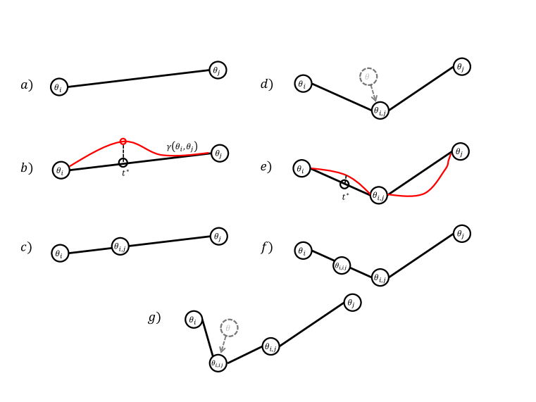
The algorithm recursively builds a string of models in the space of weights which continuously connect to . Models are added and trained until the pairwise linearly interpolated loss, i.e. for , is below the threshold, , for every pair of neighboring models on the string. We provide a cartoon of the algorithm in Appendix C.
3.2 Failure Conditions and Practicalities
While the algorithm presented will faithfully certify two models are connected if the algorithm converges, it is worth emphasizing that the algorithm does not guarantee that two models are disconnected if the algorithm fails to converge. In general, the problem of determining if two models are connected can be made arbitrarily difficult by choice of a particularly pathological geometry for the loss function, so we are constrained to heuristic arguments for determining when to stop running the algorithm. Thankfully, in practice, loss function geometries for problems of interest are not intractably difficult to explore. We comment more on diagnosing disconnections more carefully in Appendix E.
Further, if the exceeds for every new recursive branch as the algorithm progresses, the worst case runtime scales as . Empirically, we find that the number of new models added at each depth does grow, but eventually saturates, and falls for a wide variety of models and architectures, so that the typical runtime is closer to —at least up until a critical value of .
To aid convergence, either of the choices in line of the algorithm works in practice—choosing at a local maximum can provide a modest increase in algorithm runtime, but can be unstable if the the calculated interpolated loss is particularly flat or noisy. is more stable, but slower. Finally, we find that training to for in line of the algorithm tends to aid convergence without noticeably impacting our numerics. We provide further implementation details in 4.
4 Numerical Experiments
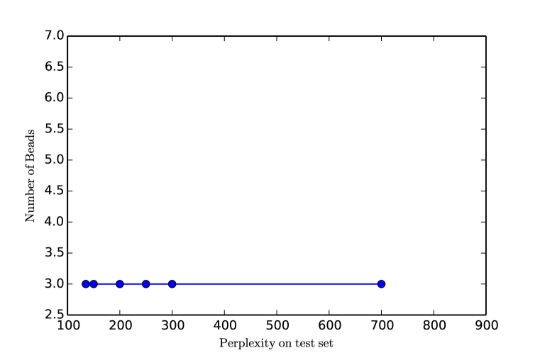
For our numerical experiments, we calculated normalized geodesic lengths for a variety of regression and classification tasks. In practice, this involved training a pair of randomly initialized models to the desired test loss value/accuracy/perplexity, and then attempting to connect that pair of models via the Dynamic String Sampling algorithm. We also tabulated the average number of “beads”, or the number intermediate models needed by the algorithm to connect two initial models. For all of the below experiments, the reported losses and accuracies are on a restricted test set. For more complete architecture and implementation details, see our GitHub page.
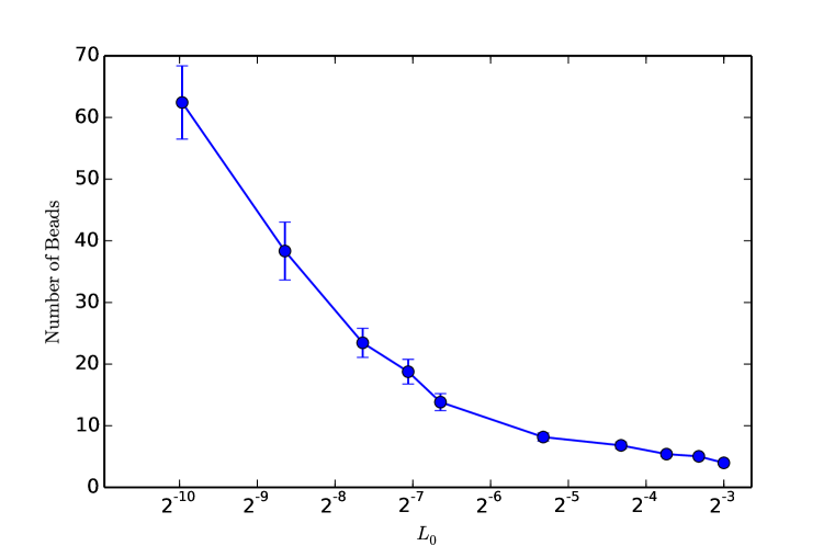
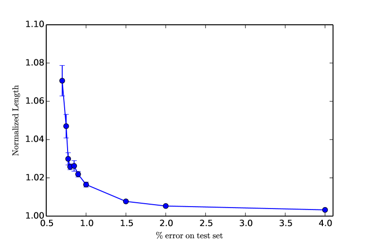
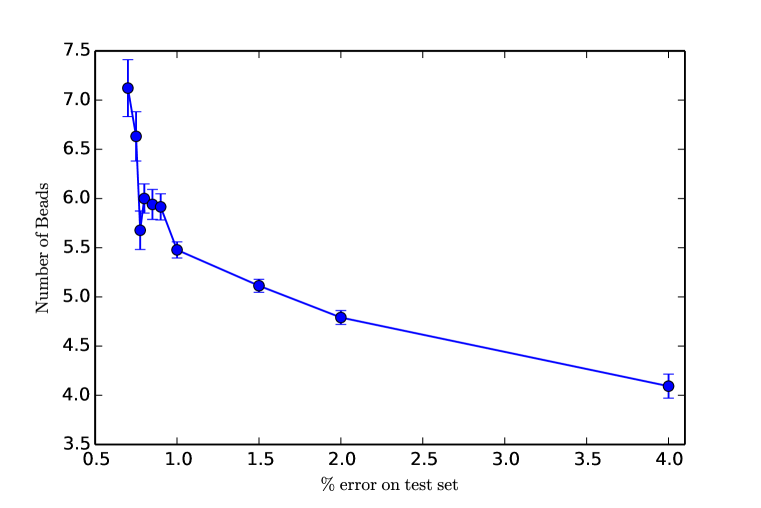
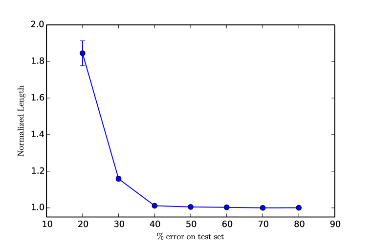
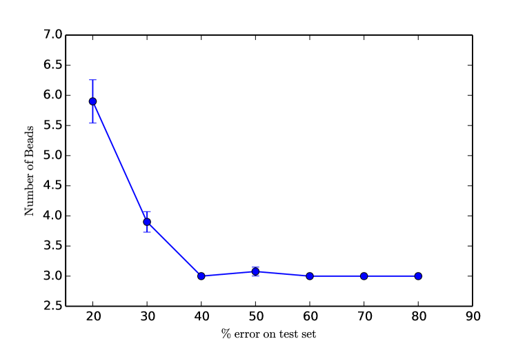
The results are broadly organized by increasing model complexity and task difficulty, from easiest to hardest. Throughout, and remarkably, we were able to easily connect models for every dataset and architecture investigated except the one explicitly constructed counterexample discussed in Appendix E.1. Qualitatively, all of the models exhibit a transition from a highly convex regime at high loss to a non-convex regime at low loss, as demonstrated by the growth of the normalized length as well as the monotonic increase in the number of required “beads” to form a low-loss connection.
4.1 Polynomial Regression
We studied a 1-4-4-1 fully connected multilayer perceptron style architecture with sigmoid nonlinearities and RMSProp/ADAM optimization. For ease-of-analysis, we restricted the training and test data to be strictly contained in the interval and . The number of required beads, and thus the runtime of the algorithm, grew approximately as a power-law, as demonstrated in Table 1 Fig. 1. We also provide a visualization of a representative connecting path between two models of equivalent power in Appendix D.
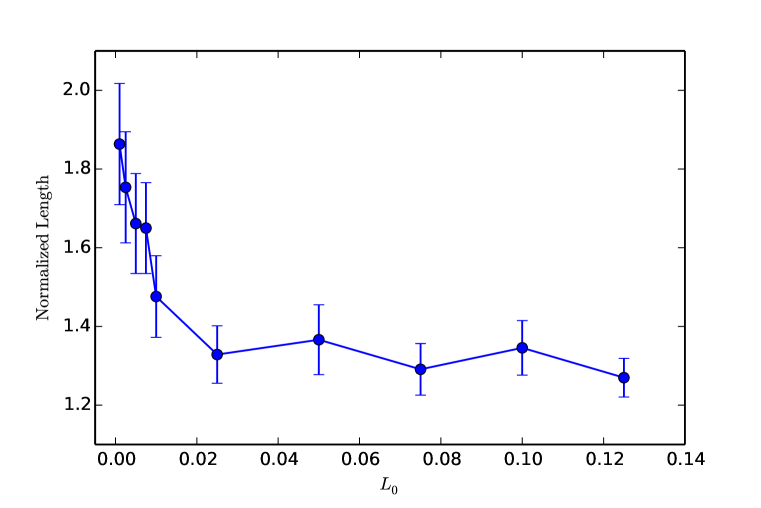
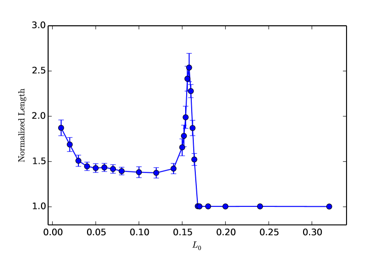
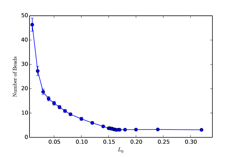
The cubic regression task exhibits an interesting feature around in Table 1 Fig. 2, where the normalized length spikes, but the number of required beads remains low. Up until this point, the cubic model is strongly convex, so this first spike seems to indicate the onset of non-convex behavior and a concomitant radical change in the geometry of the loss surface for lower loss.
4.2 Convolutional Neural Networks
To test the algorithm on larger architectures, we ran it on the MNIST hand written digit recognition task as well as the CIFAR10 image recognition task, indicated in Table 1, Figs. 3 and 4. Again, the data exhibits strong qualitative similarity with the previous models: normalized length remains low until a threshold loss value, after which it grows approximately as a power law. Interestingly, the MNIST dataset exhibits very low normalized length, even for models nearly at the state of the art in classification power, in agreement with the folk-understanding that MNIST is highly convex and/or “easy”. The CIFAR10 dataset, however, exhibits large non-convexity, even at the modest test accuracy of 80%.
4.3 Recurrent Neural Networks
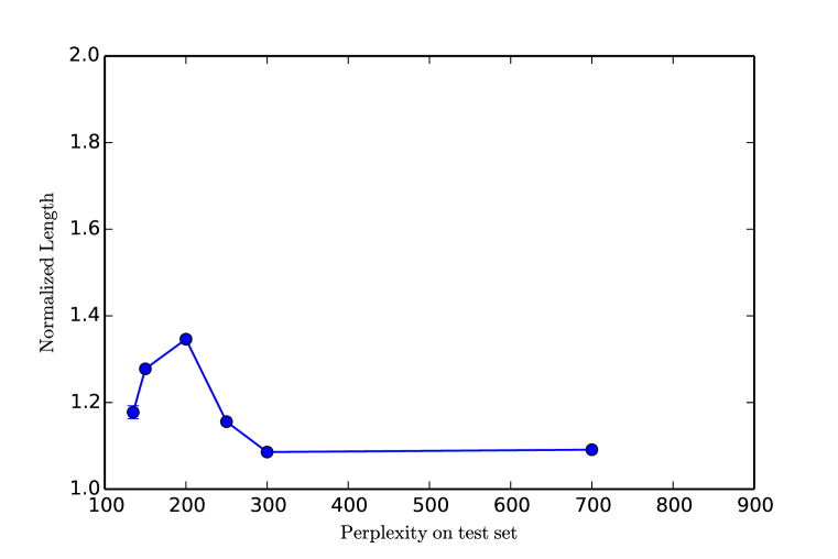
To gauge the generalizability of our algorithm, we also applied it to an LSTM architecture for solving the next word prediction task on the PTB dataset, depicted in Table 1 Fig. 5. Noteably, even for a radically different architecture, loss function, and data set, the normalized lengths produced by the DSS algorithm recapitulate the same qualitative features seen in the above datasets—i.e., models can be easily connected at high perplexity, and the normalized length grows at lower and lower perplexity after a threshold value, indicating an onset of increased non-convexity of the loss surface.
5 Discussion
We have addressed the problem of characterizing the loss surface of neural networks from the perspective of gradient descent algorithms. We explored two angles – topological and geometrical aspects – that build on top of each other.
On the one hand, we have presented new theoretical results that quantify the amount of uphill climbing that is required in order to progress to lower energy configurations in single hidden-layer ReLU networks, and proved that this amount converges to zero with overparametrization under mild conditions. On the other hand, we have introduced a dynamic programming algorithm that efficiently approximates geodesics within each level set, providing a tool that not only verifies the connectedness of level sets, but also estimates the geometric regularity of these sets. Thanks to this information, we can quantify how ‘non-convex’ an optimization problem is, and verify that the optimization of quintessential deep learning tasks – CIFAR-10 and MNIST classification using CNNs, and next word prediction using LSTMs – behaves in a nearly convex fashion up until they reach high accuracy levels.
That said, there are some limitations to our framework. In particular, we do not address saddle-point issues that can greatly affect the actual convergence of gradient descent methods. There are also a number of open questions; amongst those, in the near future we shall concentrate on:
-
•
Extending Theorem 2.4 to the multilayer case. We believe this is within reach, since the main analytic tool we use is that small changes in the parameters result in small changes in the covariance structure of the features. That remains the case in the multilayer case.
-
•
Empirical versus Oracle Risk. A big limitation of our theory is that right now it does not inform us on the differences between optimizing the empirical risk versus the oracle risk. Understanding the impact of generalization error and stochastic gradient in the ability to do small uphill climbs is an open line of research.
-
•
Influence of symmetry groups. Under appropriate conditions, the presence of discrete symmetry groups does not prevent the loss from being connected, but at the expense of increasing the capacity. An important open question is whether one can improve the asymptotic properties by relaxing connectedness to being connected up to discrete symmetry.
-
•
Improving numerics with Hyperplane method. Our current numerical experiments employ a greedy (albeit faster) algorithm to discover connected components and estimate geodesics. We plan to perform experiments using the less greedy algorithm described in Appendix A.
Acknowledgments
We would like to thank Mark Tygert for pointing out the reference to the -nets and Kolmogorov capacity, and Martin Arjovsky for spotting several bugs in early version of the results. We would also like to thank Maithra Raghu and Jascha Sohl-Dickstein for enlightening discussions, as well as Yasaman Bahri for helpful feedback on an early version of the manuscript. CDF was supported by the NSF Graduate Research Fellowship under Grant DGE-1106400.
References
- Bach, [2013] Bach, Francis. 2013. Convex relaxations of structured matrix factorizations. arXiv preprint arXiv:1309.3117.
- Choromanska et al. , [2015] Choromanska, Anna, Henaff, Mikael, Mathieu, Michael, Arous, Gérard Ben, & LeCun, Yann. 2015. The Loss Surfaces of Multilayer Networks. In: Proc. AISTATS.
- Dauphin et al. , [2014] Dauphin, Yann N, Pascanu, Razvan, Gulcehre, Caglar, Cho, Kyunghyun, Ganguli, Surya, & Bengio, Yoshua. 2014. Identifying and attacking the saddle point problem in high-dimensional non-convex optimization. Pages 2933–2941 of: Advances in Neural Information Processing Systems.
- Donoho, [2006] Donoho, David L. 2006. Compressed sensing. IEEE Transactions on information theory, 52(4), 1289–1306.
- Duchi et al. , [2011] Duchi, John, Hazan, Elad, & Singer, Yoram. 2011. Adaptive subgradient methods for online learning and stochastic optimization. Journal of Machine Learning Research, 12(Jul), 2121–2159.
- Ekanadham et al. , [2011] Ekanadham, Chaitanya, Tranchina, Daniel, & Simoncelli, Eero P. 2011. Recovery of sparse translation-invariant signals with continuous basis pursuit. IEEE transactions on signal processing, 59(10), 4735–4744.
- Goodfellow et al. , [2014] Goodfellow, Ian J, Vinyals, Oriol, & Saxe, Andrew M. 2014. Qualitatively characterizing neural network optimization problems. arXiv preprint arXiv:1412.6544.
- Hinton et al. , [2012] Hinton, Geoffrey, Srivastava, N, & Swersky, Kevin. 2012. Lecture 6a Overview of mini–batch gradient descent. Coursera Class.
- Ioffe & Szegedy, [2015] Ioffe, Sergey, & Szegedy, Christian. 2015. Batch normalization: Accelerating deep network training by reducing internal covariate shift. arXiv preprint arXiv:1502.03167.
- Kawaguchi, [2016] Kawaguchi, Kenji. 2016. Deep Learning without Poor Local Minima. arXiv preprint arXiv:1605.07110.
- Kingma & Ba, [2014] Kingma, Diederik, & Ba, Jimmy. 2014. Adam: A method for stochastic optimization. arXiv preprint arXiv:1412.6980.
- Lee et al. , [2016] Lee, Jason D, Simchowitz, Max, Jordan, Michael I, & Recht, Benjamin. 2016. Gradient descent converges to minimizers. University of California, Berkeley, 1050, 16.
- Safran & Shamir, [2015] Safran, Itay, & Shamir, Ohad. 2015. On the quality of the initial basin in overspecified neural networks. arXiv preprint arXiv:1511.04210.
- Sagun et al. , [2014] Sagun, Levent, Guney, V Ugur, Arous, Gerard Ben, & LeCun, Yann. 2014. Explorations on high dimensional landscapes. arXiv preprint arXiv:1412.6615.
- Saxe et al. , [2013] Saxe, Andrew M, McClelland, James L, & Ganguli, Surya. 2013. Exact solutions to the nonlinear dynamics of learning in deep linear neural networks. arXiv preprint arXiv:1312.6120.
- Shamir, [2016] Shamir, Ohad. 2016. Distribution-Specific Hardness of Learning Neural Networks. arXiv:1609.01037.
- Soudry & Carmon, [2016] Soudry, Daniel, & Carmon, Yair. 2016. No bad local minima: Data independent training error guarantees for multilayer neural networks. arXiv preprint arXiv:1605.08361.
- Swirszcz et al. , [2016] Swirszcz, Grzegorz, Czarnecki, Wojciech Marian, & Pascanu, Razvan. 2016. Local minima in training of neural networks. arXiv preprint arXiv:1611.06310.
- Tang et al. , [2013] Tang, Gongguo, Bhaskar, Badri Narayan, Shah, Parikshit, & Recht, Benjamin. 2013. Compressed sensing off the grid. IEEE Transactions on Information Theory, 59(11), 7465–7490.
- Tian, [2017] Tian, Yuandong. 2017. Symmetry-breaking convergence analysis of certain two-layered neural networks with ReLU nonlinearity. ICLR Workshop 2017.
- Vershynin, [2010] Vershynin, Roman. 2010. Introduction to the non-asymptotic analysis of random matrices. arXiv preprint arXiv:1011.3027.
Appendix A Constrained Dynamic String Sampling
While the algorithm presented in Sec. 3.1 is fast for sufficiently smooth families of loss surfaces with few saddle points, here we present a slightly modified version which, while slower, provides more control over the convergence of the string. We did not use the algorithm presented in this section for our numerical studies.
Instead of training intermediate models via full SGD to a desired accuracy as in step of the algorithm, intermediate models are be subject to a constraint that ensures they are “close” to the neighboring models on the string. Specifically, intermediate models are constrained to the unique hyperplane in weightspace equidistant from its two neighbors. This can be further modified by additional regularization terms to control the “springy-ness” of the string. These heuristics could be chosen to try to more faithfully sample the geodesic between two models.
In practice, for a given model on the string, , these two regularizations augment the standard loss by: . The regularization term controls the “springy-ness” of the weightstring, and the regularization term controls how far off the hyperplane a new model can deviate.
Because adapting DSS to use this constraint is straightforward, here we will describe an alternative “breadth-first” approach wherein models are trained in parallel until convergence. This alternative approach has the advantage that it will indicate a disconnection between two models “sooner” in training. The precise geometry of the loss surface will dictate which approach to use in practice.
Given two random models and where , we aim to follow the evolution of the family of models connecting to . Intuitively, almost every continuous path in the space of random models connecting to has, on average, the same (high) loss. For simplicity, we choose to initialize the string to the linear segment interpolating between these two models. If this entire segment is evolved via gradient descent, the segment will either evolve into a string which is entirely contained in a basin of the loss surface, or some number of points will become fixed at a higher loss. These fixed points are difficult to detect directly, but will be indirectly detected by the persistence of a large interpolated loss between two adjacent models on the string.
The algorithm proceeds as follows:
(0.) Initialize model string to have two models, and .
1. Begin training all models to the desired loss, keeping the instantaneous loss, , of all models being trained approximately constant.
2. If the pairwise interpolated loss between and exceeds , insert a new model at the maximum of the interpolated loss (or halfway) between these two models.
3. Repeat steps (1) and (2) until all models (and interpolated errors) are below a threshold loss , or until a chosen failure condition (see 3.2).
Appendix B Proofs
B.1 Proof of Proposition 2.1
Suppose that is a local minima and is a global minima, but . If , then clearly and both belong to . Suppose now that is connected. Then we could find a smooth (i.e. continuous and differentiable) path with , and . But this contradicts the strict local minima status of , and therefore cannot be connected .
B.2 Proof of Proposition 2.2
Let us first consider the case with . We proceed by induction over the number of layers . For , the loss is convex. Let , be two arbitrary points in a level set . Thus and . By definition of convexity, a linear path is sufficient in that case to connect and :
Suppose the result is true for . Let and with , . Since for , we can find such that . For each , we denote for and . By induction hypothesis, the loss expressed in terms of is connected between and . Let the corresponding linear path projected in the layer . We need to produce a path in the variables , such that:
-
i
, ,
-
ii
, ,
-
iii
for .
For simplicity, we denote by and the dimensions of , and assume without loss of generality that .
Suppose first that . Hence . Let , be the singular value decomposition of and respectively, with . Observe that by appropriately flipping the signs of columns of and , we can always assume that . Since has two connected components and and belong to the same one, we can find a continuous path with , and for all . Also, since by assumption, we can always complete the rectangular matrices into , such that . It follows that we can also consider a path with , and for all . In particular, since for all , the restriction of to its first columns, , has rank for all . Finally, since the singular values , are lower bounded by , we can construct a path such that is diagonal, , , and for all .
We consider the path
| (12) |
has the property that , . Thanks to the fact that for all , there exists such that
| (13) |
Finally, we need to show that the path is continuous and satisfies , . Since by construction the paths are continuous in , it only remains to be shown that
| (14) |
From (13) we have
Consider first the case . Since is continuous in a compact interval, we have . Also, , so we have
| (15) | |||||
since and are both continuous at . Analogously we have .
Finally, if either or , we denote by (resp ) the orthogonal complement of (resp ), and by (resp ) the orthogonal complement of (resp ). Observe that if either intersects with (resp intersects with ), we can shrink in the intersection with no effect in the loss. We can thus assume without loss of generality that . In that case, increasing the range of until it has rank has no effect in the loss either, since the new directions will fall in the kernel of . Therefore, by applying the necessary corrections to and (resp and ) we can reduce ourselves to the previous case.
Finally, let us prove that the result is also true when and . We construct the path using the variational properties of atomic norms [1]. When we pick the ridge regression regularization, the corresponding atomic norm is the nuclear norm:
The path is constructed by exploiting the convexity of the variational norm . Let and , and we define . Since , it results that
| (16) |
From (16) it results that the loss can be minored by another loss expressed in terms of of the form
which is convex with respect to . Thus a linear path in from to is guaranteed to be below . Let us define
One can verify that we can first consider a path from to such that
and similarly for to . The path satisfies (i-iii) by definition. We also verify that
Finally, we verify that the paths we have just created, when applied to arbitrary and a global minimum, are strictly decreasing, again by induction. For , this is again an immediate consequence of convexity. For , our inductive construction guarantees that for any , the path satisfies . This concludes the proof .
B.3 Proof of Proposition 2.3
Let
By definition, we have
| (17) | |||||
| (18) | |||||
| (19) |
where is the orthogonal projection onto the space spanned by and and is the marginal density on that subspace. Since this projection does not interfere with the rest of the proof, we abuse notation by dropping the and still referring to as the probability density.
Now, let and . By construction we have
and thus
| (20) |
By denoting , observe that . Let us denote by the disjoint complement. It results that
| (21) | |||||
We conclude by bounding each error term and separately:
| (22) |
since every point in by definition has angle greater than from . Also,
| (23) |
by direct application of Cauchy-Schwartz. The proof is completed by plugging the bounds from (22) and (23) into (B.3) .
B.4 Proof of Theorem 2.4
Consider a generic and . A path from to will be constructed by concatenating the following paths:
-
1.
from to , the best linear predictor using the same first layer as ,
-
2.
from to , the best -term approximation using perturbed atoms from ,
-
3.
from to the oracle term approximation,
-
4.
from to , the best -term approximation using perturbed atoms from ,
-
5.
from to , the best linear predictor using the same first layer as ,
-
6.
from to .
The proof will study the increase in the loss along each subpath and aggregate the resulting increase into a common bound.
Subpaths (1) and (6) only involve changing the parameters of the second layer while leaving the first-layer weights fixed, which define a convex loss. Therefore a linear path is sufficient to guarantee that the loss along that path will be upper bounded by on the first end and on the other end.
Concerning subpaths (3) and (4), we notice that they can also be constructed using only parameters of the second layer, by observing that one can fit into a single parameter matrix both the -term approximation and the oracle -term approximation. Indeed, let us describe subpath (3) in detail ( subpath (4) is constructed analogously by replacing the role of with ). Let the first-layer parameter matrix associated with the -sparse solution , and let denote its second layer coefficients, which is a -dimensional vector with at most non-zero coefficients. Let be the first-layer matrix of the -term oracle approximation, and the corresponding second-layer coefficients. Since there are only columns of that are used, corresponding to the support of , we can consider a path that replaces the remaining columns with those from while keeping the second-layer vector fixed. Since the modified columns correspond to zeros in , such paths have constant loss. Call the resulting first-layer matrix, containing both the active active columns of and the columns of in the positions determined by the zeros of . Now we can consider the linear subpath that interpolates between and while keeping the first layer fixed at . Since again this is a linear subpath that only moves second-layer coefficients, it is non-increasing thanks to the convexity of the loss while fixing the first layer. We easily verify that at the end of this linear subpath we are using the oracle -term approximation, which has loss , and therefore subpath (3) incurs in a loss that is bounded by its extremal values and .
Finally, we need to show how to construct the subpaths (2) and (5), which are the most delicate step since they cannot be bounded using convexity arguments as above. Let be the resulting perturbed first-layer parameter matrix with sparse coefficients . Let us consider an auxiliary regression of the form
and regression parameters
Clearly
and similarly for . By convexity, the augmented linear path thus satisfies
Let us now approximate this augmented linear path with a path in terms of first and second layer weights. We consider
We have that
| (24) | |||||
| (25) |
Finally, we verify that
| (26) | |||
Indeed, from Proposition 2.3, and using the fact that
we can write
with and using concavity of the moments. Thus
which proves (26).
We have just constructed a path from to , in which all subpaths except (2) and (5) have energy maximized at the extrema due to convexity, given respectively by , , , , , and . For the two subpaths (2) and (5), (26) shows that it is sufficient to add the corresponding upper bound to the linear subpath, which is of the form where is an explicit constant independent of . Since and are arbitrary, we are free to pick the infimum, which concludes the proof.
B.5 Proof of Corollary 2.5
Let us consider a generic first layer weight matrix . Without loss of generality, we can assume that for all , since increasing the norm of within the unit ball has no penalty in the loss, and we can compensate this scaling in the second layer thanks to the homogeneity of the half-rectification. Since this results in an attenuation of these second layer weights, they too are guaranteed not to increase the loss.
From [21] [Lemma 5.2] we verify that the covering number of the Euclidean unit sphere satisfies
which means that we can cover the unit sphere with an -net of size .
Let , and let us pick, for each , . Let us consider its corresponding -net of size
Since we have vectors in the unit sphere, it results from the pigeonhole principle that at least one element of the net will be associated with at least vectors; in other words, we are guaranteed to find amongst our weight vector a collection of vectors that are all at an angle at most apart. Let us now apply Theorem 2.4 by picking and . We need to see that the terms involved in the bound all converge to as .
The contribution of the oracle error goes to zero as by the fact that exists (it is a decreasing, positive sequence) and that .
Let us now verify that also converges to zero. We are going to prune the first layer by removing one by one the vectors in . Removing one of these vectors at a time incurs in an error of the order of . Indeed, let be one of such vectors and let be the solution of
where is a shorthand for the matrix containing the rest of the vectors that have not been discarded yet. Removing the vector from the first layer increases the loss by a factor that is upper bounded by , where
since now is a feasible solution for the pruned first layer.
Let us finally bound .
Since , it results from Proposition 2.3 that
with for some constant independent of . By redefining and , we have
where only depends on . We also verify that .
It results that removing of such vectors incurs an increase of the loss at most . Since we picked such that , this term converges to zero. The proof is finished.
Appendix C Cartoon of Algorithm
Refer to Fig. 2.
Appendix D Visualization of Connection
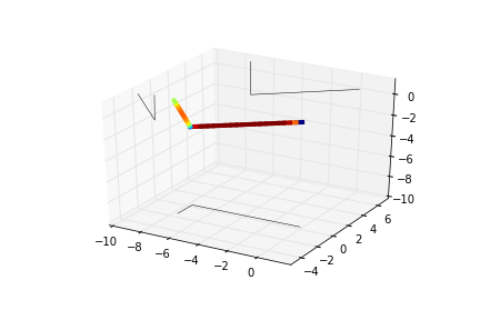
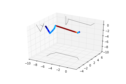
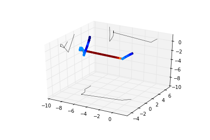
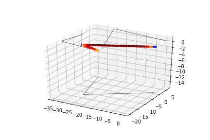
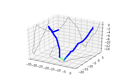
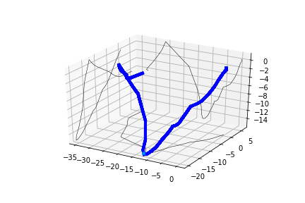
Because the weight matrices are anywhere from high to extremely high dimensional, for the purposes of visualization we projected the models on the connecting path into a three dimensionsal subspace. Snapshots of the algorithm in progress for the quadratic regression task are indicated in Fig. 3. This was done by vectorizing all of the weight matrices for all the beads for a given connecting path, and then performing principal component analysis to find the three highest weight projections for the collection of models that define the endpoints of segments for a connecting path—i.e., the discussed in the algorithm. We then projected the connecting string of models onto these three directions.
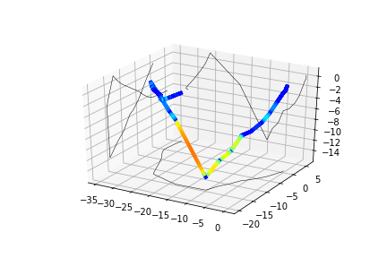
The color of the strings was chosen to be representative of the test loss under a log mapping, so that extremely high test loss mapped to red, whereas test loss near the threshold mapped to blue. An animation of the connecting path can be seen on our Github page.
Finally, projections onto pairs of principal components are indicated by the black curves.
Appendix E A Disconnection
E.1 A Disconnection
As a sanity check for the algorithm, we also applied it to a problem for which we know that it is not possible to connect models of equivalent power by the arguments of section 2.3.1. The input data is 3 points in , and the task is to permute the datapoints, i.e. map . This map requires at least 12 parameters in general for the three linear maps which take for . Our archticture was a 2-3-2 fully connected neural network with a single relu nonlinearity after the hidden layer—a model which clearly has 12 free parameters by construction. The two models we tried to connect were a single model, , and a copy of with the first two neurons in the hidden layer permuted, . The algorithm fails to converge when initialized with these two models. We provide a visualization of the string of models produced by the algorithm in Fig. 4.
In general, a persistent high interpolated loss between two neighboring beads on the string of models could arise from either a slowly converging, connected pair of models or from a truly disconnected pair of models. “Proving” a disconnection at the level of numerical experiments is intractable in general, but a collection of negative results—i.e., failures to converge—are highly suggestive of a true disconnection.
