Lens Modeling Abell 370: Crowning the Final Frontier Field with MUSE
Abstract
We present a strong lensing analysis on the massive cluster Abell 370 (A370; ), using a combination of deep multi-band Hubble Space Telescope (HST) imaging and Multi-Unit Spectroscopic Explorer (MUSE) spectroscopy. From only two hours of MUSE data, we are able to measure 120 redshifts in the Southern BCG area, including several multiply-imaged lens systems. In total, we increase the number of multiply-imaged systems with a secure redshift from 4 to 15, nine of which are newly discovered. Of these, eight are located at , greatly extending the redshift range of spectroscopically-confirmed systems over previous work. Using these systems as constraints, we update a parametric lens model of A370, probing the mass distribution from cluster to galaxy scales. Overall, we find that a model with only two cluster-scale dark matter halos (one for each BCG) does a poor job of fitting these new image constraints. Instead, two additional mass clumps – a central “bar” of mass located between the BCGs, and another clump located within a “crown” of galaxies in the Northern part of the cluster field – provide significant improvements to the fit. Additional physical evidence suggests these clumps are indeed real features of the system, but with relatively few image constraints in the crown region, this claim is difficult to evaluate from a modeling perspective. Additional MUSE observations of A370 covering the entire strong-lensing region will greatly help these efforts, further improving our understanding of this intriguing cluster.
keywords:
gravitational lensing: strong – galaxies: clusters: individual: Abell 370 – techniques: imaging spectroscopy – dark matter – galaxies: high redshift1 Introduction
Galaxy clusters acting as strong gravitational lenses are powerful astrophysical laboratories. The lensed background sources constrain the cluster mass model, providing insight into the mass environments of the densest regions of the Universe (Bradač et al., 2008a, b; Hsu, Ebeling, & Richard, 2013; Massey et al., 2015). At the same time, the cluster magnifies these sources, making them larger, brighter, and better resolved. This allows for more detailed studies of faint, low-mass, high-redshift galaxies, opening a window into the early Universe (Ebeling et al., 2009; Sharon et al., 2012; Monna et al., 2014; Patrício et al., 2016). Over the past decade, cluster lensing science has significantly expanded, and hundreds of new lensed systems have been discovered (e.g., Zitrin et al., 2011; Jauzac et al., 2015; Hoag et al., 2016; Kawamata et al., 2016). This is largely thanks to improved modeling techniques (such as Jullo et al. 2007 and Oguri 2010) and the efforts of deep, high-resolution imaging campaigns (e.g., Postman et al., 2012; Schmidt et al., 2014; Lotz et al., 2016), driven primarily by the Hubble Space Telescope (HST).
But while these imaging campaigns are able to identify and resolve background sources like never before, imaging alone does not provide high-precision () redshift information, a crucial component in interpreting models and deriving their physical values. While some spectroscopic campaigns are underway (e.g., Rosati et al., 2014; Treu et al., 2015), acquiring spectra of lensed systems has, to date, largely been a long, costly, and inefficient process. With the advent of Integral Field Unit (IFU) spectroscopy, however, this situation is rapidly changing. Leading the way in these efforts is the Multi-Unit Spectroscopic Explorer (MUSE; Bacon et al. 2010) a wide-field IFU on the Very Large Telescope (VLT) in Chile. With a large arcmin2 field of view and high sensitivity between 4800 and 9300 Å, MUSE is an incredibly efficient redshift engine, providing several hundred redshifts between and in only a few hours of exposure time (e.g. Bacon et al., 2015). As an IFU, MUSE is also well-suited for blind redshift surveys, able to detect emission lines from continuum-free sources without pre-selecting a redshift range. These objects (which are often missed in traditional broad-band imaging campaigns) include high-redshift, lensed Lyman- emitters. This has been, unsurprisingly, a boon to the lensing community, and some studies have already begun to take advantage of MUSE data (e.g., Karman et al., 2015; Richard et al., 2015; Bina et al., 2016; Jauzac et al., 2016; Caminha et al., 2016).
In this work, we present new MUSE data of the strong lensing cluster Abell 370 (A370; Abell 1958). A370 is a massive cluster (; Umetsu et al. 2011) at redshift (Mellier et al., 1988) with historical significance to lensing: it contains one of the first known “Giant Luminous Arc” features (Lynds & Petrosian, 1986), which later became the first spectroscopically-confirmed giant-arc lens system (Soucail et al., 1987, 1988; Lynds & Petrosian, 1989). Thanks to this discovery, and the identification of other lensed features (Fort et al., 1988; Mellier et al., 1991; Kneib et al., 1993), A370 became an important benchmark in the early days of lens modeling (e.g., Kneib et al., 1993; Smail et al., 1996; Bézecourt et al., 1999a, b). However, after an initial period of activity, interest in A370 slowly waned; there was little spectroscopic follow-up on the cluster, and it was not selected to be a part of massive cluster surveys such as MACS (Ebeling, Edge, & Henry, 2001) or CLASH (Postman et al., 2012), in spite of its high X-ray luminosity ( erg s-1; Morandi, Ettori, & Moscardini 2007).
In 2010, a newly-refurbished HST observed A370 to test its deep-imaging capabilities, generating renewed interest. This led to a new lens model (Richard et al., 2010), additional weak-lensing analyses (Medezinski et al., 2011; Umetsu et al., 2011), and its eventual selection as one of the Hubble Frontier Fields (HFF) clusters (Lotz et al., 2016). Several groups have since modeled the cluster (see the HFF archive111https://archive.stsci.edu/pub/hlsp/frontier/abell370/models/ and also Richard et al. 2014 and Johnson et al. 2014), but (until recently) only three lensed systems have had a secure redshift, all with (see section 3.1.1 for details.) As a result, these models are only able to probe the critical line region of the cluster out to small radii. While recent work by Diego et al. (2016) has increased the number of secure-redshift systems to five, the highest of these is still . Here, we extend the redshift range of spectroscopically-confirmed systems even further and present newly-discovered systems as well. By combining the MUSE spectroscopy with the current HFF data, we can therefore improve on existing lens models, probing the mass distribution out to larger scales and with much higher precision. In this way, we can improve our view of this massive cluster in conjunction with the final HFF data release.
Overall, this work is organized as follows: In Section 2, we describe the MUSE and HFF data and the data reduction processes we used. In Section 3, we describe how we extract MUSE redshifts and present the A370 redshift catalog, paying particular attention to redshifts of the multiply-imaged galaxies. Using these redshifts, we construct a new mass model, which we present in Section 4. We discuss the results of the mass modeling and make predictions for future work in Section 5. Finally, we briefly conclude in Section 6. Throughout this paper, we assume a standard cosmological model with , , and = 70 km s-1 Mpc-1. Using this model, one arcsecond covers a physical distance of 5.162 kpc at the A370 redshift (). All magnitudes are measured using the AB system.
2 Data
Lensing is a three-dimensional effect, sensitive to both the transverse and line-of-sight distances between objects. Therefore, we need a combination of imaging data (to identify lensed objects and measure their apparent positions) and redshift data (to measure radial distances) to construct an accurate lens model of A370.
2.1 HST Imaging
HST imaging data of A370 were taken as part of the Hubble Frontier Fields (HFF) Program, and are publicly available on the HFF website222http://www.stsci.edu/hst/campaigns/frontier-fields/. While the imaging campaign for A370 is now complete, the Epoch 1 (v1.0) mosaics that we use in this work consist of deep Advanced Camera for Surveys (ACS; Ford et al. 2003) data in three optical bands, F435W, F606W, and F814W (ID: 13504, PI: J. Lotz). These are supplemented by shallower F814W imaging from archival programs: (ID: 11507, PI: K. Noll) and (ID: 11591, PI J.-P. Kneib). Additionally, shallow, archival, Wide-Field Camera 3 (WFC3; Kimble et al. 2008) data is available in three bands: F105W (ID: 13459, PI: T. Treu), F140W (ID: 11108, PI: E. Hu; ID: 13459, PI: T. Treu), and F160W (ID: 11591, PI: J.-P. Kneib; ID: 14216, PI: R. Kirshner), and a shallow, pilot HFF exposure, also in the F140W band.
Individual exposures are reduced and stacked by the HFF team directly, using the standard Pyraf/STSDAS pipeline. Additionally, the ACS mosaics are further corrected with a “self-calibration” technique to eliminate Charge Transfer Inefficiency (CTI) effects and low-level pixel noise333http://www.stsci.edu/hst/acs/software/Selfcal (J. Anderson, in prep). The full reduction procedure is described in the A370 HFF data archive444https://archive.stsci.edu/pub/hlsp/frontier/abell370/images/hst/v1.0-epoch1/hlsp_frontier_hst_acs-00_abell370_v1.0-epoch1_readme.pdf.
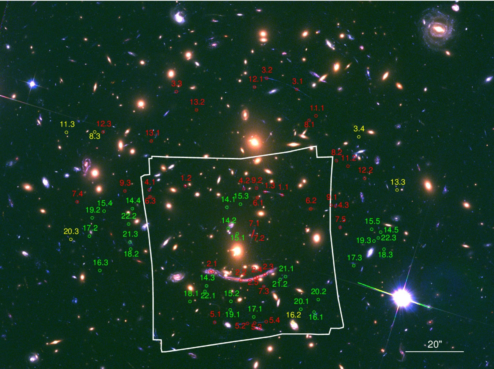
After combining all exposures, total integration times are 51400, 25316, 130643, 2335, 12894, and 9647 seconds for the F435W, F606W, F814W, F105W, F140W, and F160W bands, respectively. This is equivalent to 20, 10, 52, 1, 5, and 4 HST orbits. Collectively, this represents one of the deepest, highest resolution imaging of A370 ever taken, and corresponds to average limiting magnitudes of 29.3 in the optical bands and 27.6 in the near-IR bands. A color image of the cluster field consisting of the F435W, F606W, and F814W mosaics is shown in Figure 1.
2.2 MUSE Spectroscopy
MUSE observations of A370 were taken on UT 2014 November 20, as part of the Guaranteed Time Observing (GTO) Program 094.A-0115(A) (PI:Richard). In total, we observed four 30-minute exposures in WFM-NOAO-N mode, centered at ( , ). We applied a small ( 0.5″) dither pattern between exposures to average out systematics on the detector, and we alternated taking exposures between PA = 0° and PA = 8° to reduce the systematic striping pattern caused by the IFU image slicers. The full observational footprint can be seen in Figure 1. Typical seeing during the observations was 0.75″, as measured by stars in the field.
The raw data were reduced through the MUSE pipeline (Weilbacher et al., 2012, 2014) provided by ESO (version 1.2). This pipeline performs all basic reduction techniques: bias and flat-field correction (using a combination of internal flats and illumination and twilight exposures), wavelength and geometric calibration, sky subtraction, flux calibration, and telluric correction. The A370 data were flux-calibrated using a combination of several standard stars observed under photometric conditions. After basic corrections we align individual exposures to a common WCS with SCAMP (Bertin, 2006), shifting each frame relative to a reference image, which in this case is the F814W HFF data. We then transform the re-aligned images into data cubes, resampling all pixels onto a common 3-dimensional grid with two spatial and one spectral axis. The final spectral resolution of the cubes varies from R=2000 to R=4000, with a spectral range between 4750 and 9350 Å. To ensure that cubes are properly Nyquist-sampled, we set the wavelength grid to 1.25 Åpixel-1. The final spatial resolution is 0.2″pixel-1 in order to properly sample the PSF.
Next, we process each cube with the Zurich Atmosphere Purge (ZAP; Soto et al. 2016), a software package that uses a principal component analysis technique to remove known systematics from the sky model, further improving sky-subtraction residuals. To account for changes in sky transmittance from exposure to exposure, we compare the fluxes of stars common to each cube. The cube with the brightest flux values is taken as a new photometric standard, and we scale the zeropoints of the other cubes until the fluxes agree across all exposures. We then merge all cubes together to create a combined master cube. During the merging process, we apply a 3- clipping routine to reject outliers, eliminating cosmic-ray strikes and hot pixels on the detector. As a final step, we re-run the ZAP process on the master cube in order to eliminate low-level sky residuals that can only be seen in the improved signal-to-noise ratio of the combined data.
3 Redshift Measurement and Spectroscopic Catalog
After reducing the data, we probe the MUSE cube for redshifts using two complementary techniques: 1.) an automated emission line detection program, and 2.) a customized, interactive data visualization tool designed to extract MUSE aperture spectra by hand.
The automated program, MUSELET555http://mpdaf.readthedocs.io/en/latest/muselet.html, is included as part of the Muse Python Data Analysis Framework (MPDAF666https://git-cral.univ-lyon1.fr/MUSE/mpdaf) version 2.0. It first creates narrow-band images of the data, averaging the flux over a narrow emission wavelength range and then subtracting a local continuum. For the A370 cube, we choose an emission window of 6.25 Å (spanning five MUSE wavelength slices), with each window centered on one of the original wavelength planes. The continuum is created by averaging two 25 Å slices, immediately blue- and red-ward of the emission window. After creating the narrow-band images, MUSELET uses Source Extractor (Bertin & Arnouts, 1996) to identify emission features in each image, then merges these features together into a final master catalog. Emission features at different wavelengths are considered to belong to the same source if they fall within 0.8″ of each other (i.e., within the seeing FWHM) in the case of continuum-free detections, or if they fall within half of the effective radius (/2) of a continuum-emission object. For every source that has multiple emission lines identified, MUSELET fits a redshift using a template of known spectral lines. To ensure the accuracy of the MUSELET fit, we manually inspect the line features of each identified redshift before adding it to the final catalog.
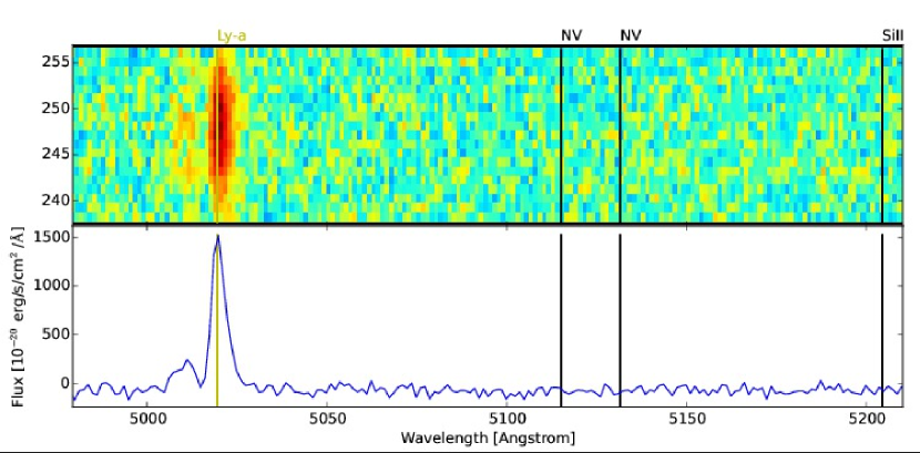
In cases where an obvious galaxy appears in the HST image or MUSE cube but is undetected (absorption galaxies) or unclassified (single emission-line galaxies) by MUSELET, we instead use the interactive tool. The tool, a custom-made Python script, collapses the data cube along the wavelength axis, creating a “white-light” image of the field. A second panel, matched to the WCS of the cube, shows a corresponding HST image to help identify the target galaxy. Once a galaxy has been identified, a user can draw a (circular or rectangular) aperture around the target object, which will extract both a 2D and 1D spectrum from the cube. From these spectra, the user can then interactively fit a redshift to the galaxy, using the same set of lines as the automatic line-finder. An example of this process can be seen in Figure 2. As an additional check, we run AutoZ (Baldry et al., 2014) on the extracted 1D spectrum. In all cases, we find the difference between the manual and AutoZ fits to be less than
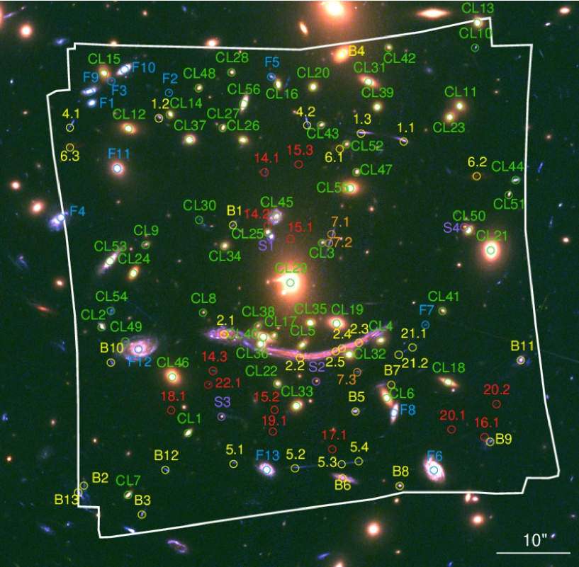
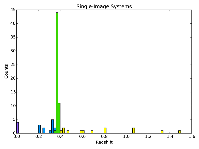
After running both methods on the A370 cube, we combine all of the redshift results into a final catalog. Overall, we securely identify 120 redshifts, consisting of multiply-imaged systems, cluster members, foreground interlopers, background sources, and stars. The spatial and spectral distributions of these redshifts are shown in Figure 3.
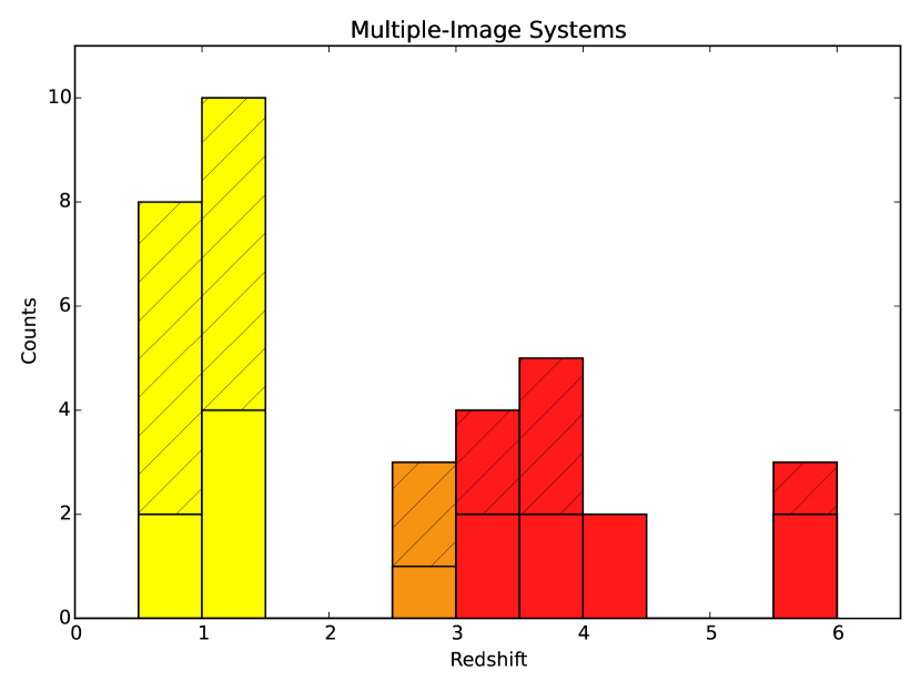
3.1 Multiply-Imaged Systems
Multiply-imaged background sources are particularly important in this work, since they provide strong constraints on the lensing mass model (see Section 4). Using a combination of HFF imaging and MUSE spectroscopy, we are able to identify and confirm the redshifts of previously known multi-image systems and identify new systems as well.
3.1.1 Previously Known Systems
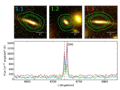
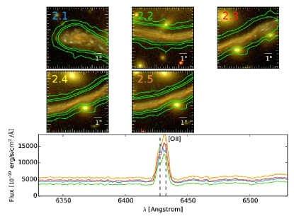
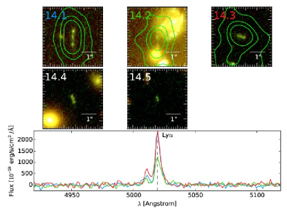
Prior to the release of the newest HFF and MUSE data, 13 multi-image objects were identified in the A370 field (Richard et al., 2014) including three with known redshifts: Systems 1 (Kneib et al., 1993), 2 (Soucail et al., 1988), and 6 (Richard et al., 2014). A tentative guess for System 4 () using VLT/FORS2 grism spectroscopy was also presented in (Richard et al., 2014). Of these systems, seven have at least one image that falls within the MUSE A370 footprint: Systems 1, 2, 4, 5, 6, 7, and 9. Using the MUSE data, we are able to confirm the previous redshifts of Systems 1 (), 2 (), and 6 (), refine and secure the redshift for System 4 (), and provide new redshifts for Systems 5 () and 7 (). We note that these new redshifts are within 2- of the values predicted in the Richard et al. (2014) lens model (System 4: ; System 5: ; System 7: ), a reasonably good agreement. We are unable to identify any strong features in System 9 because it is too faint for a secure measurement. However, Diego et al. (2016) identify [OII] and [OIII] features for the system in HST grism spectroscopy, placing it at We note that this redshift is consistent with a non-detection in MUSE, since it falls in the “redshift desert” where no strong emission features appear in the MUSE wavelength range. Additionally, Diego et al. (2016) also identify faint [OIII] emission for System 3 at . We adopt these redshift values in this work, also.
3.1.2 New Systems
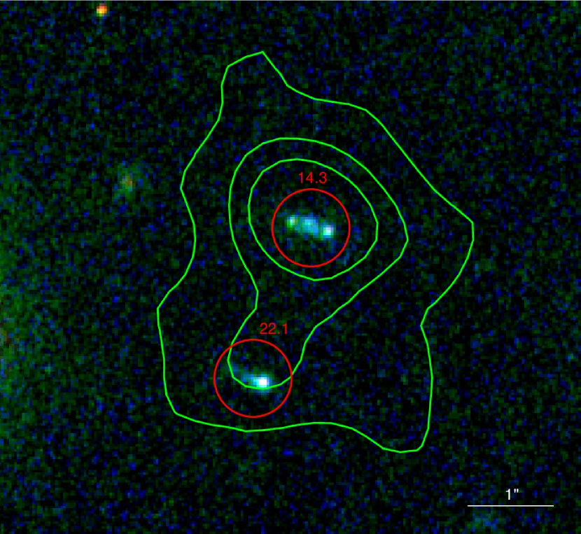
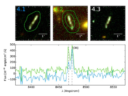
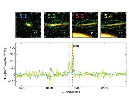
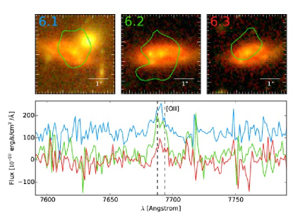
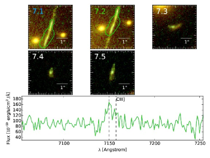
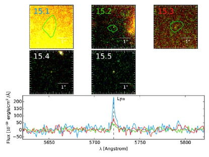
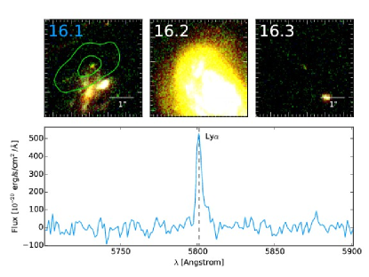
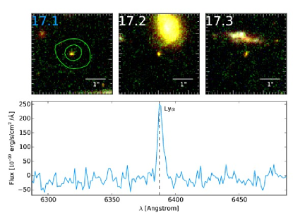
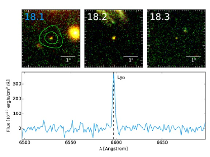
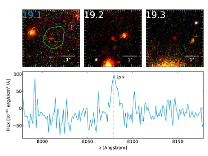
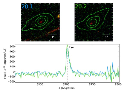
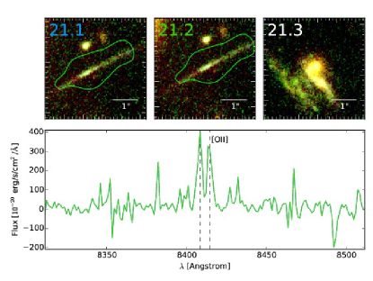
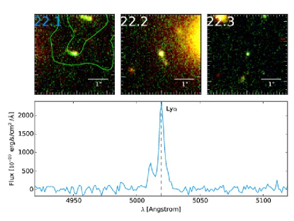
In addition to the known objects, we also identify nine new multiply-imaged systems in the MUSE field (Systems 14 – 22). Diego et al. (2016) independently identify four of these systems: 14, 20, 21, and 22 (labeled Systems 10, 29, 26, and 18, respectively, in their work) though without spectroscopic redshifts. With the exception of System 21 (identified by [OII]), these new systems are all strong Lyman- emitters, located at considerably higher redshifts () than those previously identified. Systems 14 and 22 are particularly interesting, as they are reasonably close together and have an identical redshift (). This suggests that they could be an interacting pair of galaxies, and indeed, narrow-band imaging shows that the emission-line regions of the two are clearly overlapping (Figure 4.) Careful observation of the HFF data reveals at least some flux associated with each of the new systems in broadband imaging, but in some cases – especially Systems 15 and 16 – this flux is extremely faint and contaminated by brighter objects nearby. Spectra of all systems in the MUSE field of view are shown in Figure 5. The full list of multiply-imaged systems, including all identified and/or model-predicted counterimages of a given system, is presented in Table 1.
| ID | RA | Dec | range | |
| 1.1 | 39.967047 | -1.5769172 | 0.8041 | |
| 1.2 | 39.976273 | -1.5760558 | 0.8041 | |
| 1.3 | 39.968691 | -1.5766113 | 0.8041 | |
| 2.1 | 39.973825 | -1.5842290 | 0.7251 | |
| 2.2 | 39.971003 | -1.5850422 | 0.7251 | |
| 2.3 | 39.968722 | -1.5845058 | 0.7251 | |
| 2.4 | 39.969394 | -1.5847328 | 0.7251 | |
| 2.5 | 39.969630 | -1.5848508 | 0.7251 | |
| 3.1 | 39.965658 | -1.5668560 | 1.95 d | |
| 3.2 | 39.968526 | -1.5657906 | 1.95 d | |
| 3.3 | 39.977293 | -1.5672022 | 1.95 d | |
| 3.4 | 39.959758 | -1.5713806 | – | |
| 4.1 | 39.979704 | -1.5764364 | 1.2728 | |
| 4.2 | 39.970688 | -1.5763221 | 1.2728 | |
| 4.3 | 39.961971 | -1.5779671 | 1.2728 | |
| 5.1 | 39.973473 | -1.5890463 | 1.2775 | |
| 5.2 | 39.971110 | -1.5892363 | 1.2775 | |
| 5.3 | 39.969472 | -1.5890961 | 1.2775 | |
| 5.4 | 39.968580 | -1.5890045 | 1.2775 | |
| 6.1 | 39.969405 | -1.5771811 | 1.0633 | |
| 6.2 | 39.964334 | -1.5782307 | 1.0633 | |
| 6.3 | 39.979641 | -1.5770904 | 1.0633 | |
| 7.1 | 39.969788 | -1.5804299 | 2.7512 | |
| 7.2 | 39.969882 | -1.5807608 | 2.7512 | |
| 7.3 | 39.968815 | -1.5856313 | 2.7512 | |
| 7.4 | 39.986567 | -1.5775688 | – | |
| 7.5 | 39.961533 | -1.5800028 | – | |
| *8.1 | 39.964485 | -1.5698065 | {2.042} | [0.5 – 5.0] |
| 8.2 | 39.961889 | -1.5736473 | {2.042} | |
| *8.3 | 39.984904 | -1.5709139 | {2.042} | |
| 9.1 | 39.962402 | -1.5778911 | 1.52 d | |
| 9.2 | 39.969486 | -1.5762654 | 1.52 d | |
| 9.3 | 39.982022 | -1.5765337 | 1.52 d | |
| *10.1 | 39.968585 | -1.5717898 | – | |
| 10.2 | 39.968017 | -1.5708820 | – | |
| *11.1 | 39.963839 | -1.5693802 | {4.667} | [2.5 – 10.0] |
| 11.2 | 39.960789 | -1.5741702 | {4.667} | |
| *11.3 | 39.987592 | -1.5709501 | {4.667} |
| ID | RA | Dec | range | |
|---|---|---|---|---|
| *12.1 | 39.969682 | -1.5666360 | {2.858} | [0.5 – 5.0] |
| 12.2 | 39.959198 | -1.5753221 | {2.858} | |
| 12.3 | 39.984100 | -1.5709127 | {2.858} | |
| *13.1 | 39.979513 | -1.5717782 | {5.119} | [0.5 – 5.0] |
| 13.2 | 39.975210 | -1.5688203 | {5.119} | |
| *13.3 | 39.956112 | -1.5764444 | {5.119} | |
| 14.1 | 39.972309 | -1.5780910 | 3.1309 | |
| 14.2 | 39.972192 | -1.5801027 | 3.1309 | |
| 14.3 | 39.974254 | -1.5855770 | 3.1309 | |
| 14.4 | 39.981313 | -1.5782202 | – | |
| 14.5 | 39.957673 | -1.5804590 | – | |
| 15.1 | 39.971328 | -1.5806040 | 3.7084 | |
| 15.2 | 39.971935 | -1.5870512 | 3.7084 | |
| 15.3 | 39.971027 | -1.5777907 | 3.7084 | |
| 15.4 | 39.984017 | -1.5784514 | – | |
| 15.5 | 39.958410 | -1.5793722 | – | |
| 16.1 | 39.964016 | -1.5880782 | 3.7743 | |
| *16.2 | 39.966037 | -1.5890355 | – | |
| 16.3 | 39.984414 | -1.5841111 | – | |
| 17.1 | 39.969758 | -1.5885333 | 4.2567 | |
| 17.2 | 39.985403 | -1.5808406 | – | |
| 17.3 | 39.960235 | -1.5836508 | – | |
| 18.1 | 39.975830 | -1.5870613 | 4.4296 | |
| 18.2 | 39.981476 | -1.5820728 | – | |
| 18.3 | 39.957362 | -1.5820861 | – | |
| 19.1 | 39.971996 | -1.5878654 | 5.6493 | |
| 19.2 | 39.985142 | -1.5790944 | – | |
| 19.3 | 39.958316 | -1.5813093 | – | |
| 20.1 | 39.965279 | -1.5878055 | 5.7505 | |
| 20.2 | 39.963619 | -1.5868798 | 5.7505 | |
| 20.3 | 39.986651 | -1.5812606 | – | |
| 21.1 | 39.966733 | -1.5846943 | 1.2567 | |
| 21.2 | 39.967252 | -1.5849694 | 1.2567 | |
| 21.3 | 39.981539 | -1.5814028 | – | |
| 22.1 | 39.974406 | -1.5861017 | 3.1309 | |
| 22.2 | 39.981675 | -1.5796852 | – | |
| 22.3 | 39.957906 | -1.5810108 | – |
a Images labeled with an asterisk (*) fall outside of the MUSE cube and do not have secure redshifts. We identify them in the HFF data, using the A370 mass model as a guide.
b Images in italics are predicted by the model, but no suitable counterimage is seen in HST data. We do not include these images as model constraints, but we present them here for completeness. Image 16.2, which is in the MUSE field of view but predicted to fall behind a bright cluster galaxy, is also included here, since it is undetected in MUSE.
c Redshifts enclosed in braces ({}) are fit by the model as free parameters. The fit range is given in the “ range” column.
d Redshifts for these systems are taken from Diego et al. (2016)
3.2 Cluster Members
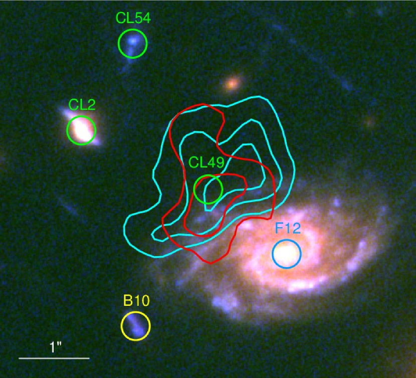
Cluster members make up the largest subgroup in the spectroscopic catalog, with 56 confirmed redshifts. To identify cluster members, we select all galaxies that fall between and , a km s-1 cut in velocity space centered on the A370 central redshift (). In the overall redshift catalog, these boundaries naturally separate the cluster overdensity from all other objects, and a large fraction of galaxies in this range fall on both the (F435W - F606W) and (F606W - F814W) red sequences. While a majority of objects are passive, elliptical galaxies showing only absorption features, some do show strong [OII], [OIII], and/or H emission. Of these emission-line galaxies, CL49 (located close to the bright, foreground spiral F12) is unique, as it is the only detected cluster member in the MUSE field of view without an HST counterpart (Figure 6.) Strangely, the object also appears to have a divergent velocity field: moving in either direction along the long axis, the flux becomes more and more redshifted relative to the center. We do not have an explanation for this behavior at this time, though it would be interesting to revisit in future work.
Cluster galaxy positions are represented by green circles in the top panel of Figure 3. The redshifts themselves are presented in Table 2.
| ID | RA | Dec | z | Type | |||
|---|---|---|---|---|---|---|---|
| Cl1 | 39.975198 | -1.5879282 | 0.3582 | 23.98 | 22.31 | 21.55 | Ca ii H, K |
| Cl2 | 39.978460 | -1.5839292 | 0.3606 | 24.16 | 22.96 | 22.34 | H |
| Cl3 | 39.970141 | -1.5807560 | 0.3609 | 25.56 | 24.02 | 23.18 | Ca ii H, K |
| Cl4 | 39.967945 | -1.5844368 | 0.3624 | 24.47 | 22.56 | 21.59 | Ca ii H, K |
| Cl5 | 39.970898 | -1.5846121 | 0.3635 | 24.52 | 22.54 | 21.59 | Ca ii H, K |
| Cl6 | 39.967716 | -1.5866033 | 0.3639 | 22.83 | 20.89 | 19.86 | Ca ii H, K |
| Cl7 | 39.977458 | -1.5902598 | 0.3645 | 24.27 | 22.71 | 21.99 | Ca ii H, K |
| Cl8 | 39.974634 | -1.5833866 | 0.3648 | 26.09 | 24.55 | 23.72 | Ca ii H, K |
| Cl9 | 39.976794 | -1.5808331 | 0.3649 | 25.41 | 23.76 | 23.00 | Ca ii H, K |
| Cl10 | 39.964373 | -1.5734012 | 0.3660 | 23.18 | 21.25 | 20.29 | Ca ii H, K |
| Cl11 | 39.964968 | -1.5756005 | 0.3660 | 23.42 | 21.40 | 20.41 | Ca ii H, K |
| Cl12 | 39.977446 | -1.5764519 | 0.3680 | 23.16 | 21.07 | 20.02 | Ca ii H, K |
| Cl13 | 39.964290 | -1.5724542 | 0.3681 | 23.18 | 21.25 | 20.29 | Ca ii H, K |
| Cl14 | 39.975885 | -1.5759172 | 0.3683 | 24.37 | 22.42 | 21.41 | Ca ii H, K |
| Cl15 | 39.978375 | -1.5743572 | 0.3683 | 23.68 | 21.53 | 20.49 | Ca ii H, K |
| Cl16 | 39.971815 | -1.5747844 | 0.3685 | 23.54 | 21.84 | 20.92 | Ca ii H, K |
| Cl17 | 39.971961 | -1.5842487 | 0.3687 | 25.34 | 23.30 | 22.30 | Ca ii H, K |
| Cl18 | 39.965402 | -1.5860164 | 0.3701 | 23.19 | 21.18 | 20.15 | Ca ii H, K |
| Cl19 | 39.969599 | -1.5837975 | 0.3708 | 22.67 | 20.66 | 19.66 | H |
| Cl20 | 39.970497 | -1.5748780 | 0.3708 | 24.06 | 22.01 | 21.01 | Ca ii H, K |
| Cl21 | 39.963783 | -1.5810351 | 0.3710 | 21.76 | 19.82 | 18.81 | Ca ii H, K |
| Cl22 | 39.971829 | -1.5860732 | 0.3711 | 24.65 | 22.77 | 21.87 | Ca ii H, K |
| Cl23 | 39.965344 | -1.5760183 | 0.3716 | 23.62 | 21.57 | 20.54 | Ca ii H, K |
| Cl24 | 39.977262 | -1.5819075 | 0.3718 | 23.37 | 21.18 | 20.07 | Ca ii H, K |
| Cl25 | 39.972201 | -1.5803644 | 0.3727 | 24.83 | 23.12 | 22.24 | Ca ii H, K |
| Cl26 | 39.973141 | -1.5768829 | 0.3728 | 23.88 | 21.94 | 20.95 | Ca ii H, K |
| Cl27 | 39.973889 | -1.5764248 | 0.3728 | 25.00 | 23.21 | 22.25 | Ca ii H, K |
| Cl28 | 39.973560 | -1.5743250 | 0.3728 | 25.05 | 23.17 | 22.19 | Ca ii H, K |
| Cl29 | 39.971337 | -1.5822570 | 0.3731 | 22.00 | 19.74 | 18.66 | Ca ii H, K |
| Cl30 | 39.974778 | -1.5798886 | 0.3738 | 25.44 | 24.60 | 24.26 | H |
| Cl31 | 39.968403 | -1.5746894 | 0.3742 | 22.96 | 20.99 | 19.95 | Ca ii H, K |
| Cl32 | 39.969132 | -1.5849674 | 0.3742 | 23.58 | 21.57 | 20.52 | Ca ii H, K |
| Cl33 | 39.971118 | -1.5869043 | 0.3749 | 23.13 | 21.16 | 20.12 | Ca ii H, K |
| Cl34 | 39.973823 | -1.5808796 | 0.3753 | 24.39 | 22.47 | 21.51 | Ca ii H, K |
| Cl35 | 39.970597 | -1.5837833 | 0.3756 | 23.83 | 21.72 | 20.67 | Ca ii H, K |
| Cl36 | 39.972478 | -1.5845667 | 0.3756 | 23.01 | 21.05 | 20.07 | Ca ii H, K |
| Cl37 | 39.975144 | -1.5768716 | 0.3762 | 23.08 | 21.21 | 20.25 | Ca ii H, K |
| Cl38 | 39.968075 | -1.5756317 | 0.3766 | 23.74 | 21.77 | 20.76 | Ca ii H, K |
| Cl39 | 39.972565 | -1.5838926 | 0.3783 | 23.01 | 21.05 | 20.07 | Ca ii H, K |
| Cl40 | 39.972358 | -1.5843052 | 0.3784 | 23.01 | 21.05 | 20.07 | Ca ii H, K |
| Cl41 | 39.965603 | -1.5833191 | 0.3789 | 25.22 | 23.43 | 22.49 | Ca ii H, K |
| Cl42 | 39.967642 | -1.5734009 | 0.3795 | 25.21 | 23.46 | 22.48 | Ca ii H, K |
| Cl43 | 39.970183 | -1.5763142 | 0.3798 | 25.13 | 23.40 | 22.46 | Ca ii H, K |
| Cl44 | 39.962843 | -1.5783866 | 0.3802 | 24.52 | 23.60 | 23.25 | H |
| Cl45 | 39.971870 | -1.5797518 | 0.3807 | 22.85 | 21.71 | 21.07 | H |
| Cl46 | 39.975789 | -1.5858086 | 0.3810 | 22.52 | 20.37 | 19.29 | Ca ii H, K |
| Cl47 | 39.968845 | -1.5780882 | 0.3826 | 24.96 | 22.98 | 21.98 | Ca ii H, K |
| Cl48 | 39.974799 | -1.5749206 | 0.3839 | 25.04 | 23.02 | 22.01 | Ca ii H, K |
| Cl49 | 39.977573 | -1.5844846 | 0.3843 | 26.76 | 26.11 | 25.62 | [OII] |
| Cl50 | 39.964628 | -1.5802868 | 0.3844 | 23.74 | 21.76 | 20.73 | Ca ii H, K |
| Cl51 | 39.963103 | -1.5789205 | 0.3848 | 25.57 | 23.82 | 23.03 | Ca ii H, K |
| Cl52 | 39.969230 | -1.5770399 | 0.3855 | 24.12 | 23.14 | 22.30 | Ca ii H, K |
| Cl53 | 39.978147 | -1.5814394 | 0.3873 | 22.20 | 20.84 | 20.12 | H |
| Cl54 | 39.978109 | -1.5833172 | 0.3873 | 24.16 | 22.96 | 22.34 | H |
| Cl55 | 39.969088 | -1.5786944 | 0.3885 | 22.74 | 20.54 | 19.46 | Ca ii H, K |
| Cl56 | 39.973107 | -1.5755088 | 0.3905 | 22.91 | 21.26 | 20.53 | Ca ii H, K |
a Listed emission/absorption lines refer to the most prominent features seen in the galaxy’s spectrum.
3.3 Other Objects
In addition to cluster members and multiply-imaged systems, the catalog also contains a number of foreground objects and singly-imaged background objects at various redshifts. We identify four stars within the MUSE field of view, mostly located near the BCG. Beyond the Milky Way, we find 13 galaxies in the foreground of the cluster, between and . Nearly all of these objects are optically blue and have emission features, in particular a very strong H- line. However, object F11 () shows strong absorption line features, with only weak [OII] emission. Behind the cluster, we find an additional 13 objects at redshifts between and . Here again, these systems are largely identified by strong [OII] and/or [OIII] emission lines, however object B4 () is another absorption-line galaxy showing weak [OII] emission. Information on all singly-imaged objects can be found in Table 3.
| ID | RA | Dec | z | Type |
|---|---|---|---|---|
| S1 | 39.972077 | -1.5805308 | 0.0000 | |
| S2 | 39.970365 | -1.5859742 | 0.0000 | |
| S3 | 39.973933 | -1.5873072 | 0.0000 | |
| S4 | 39.964779 | -1.5801536 | 0.0000 | |
| F1 | 39.978832 | -1.5754827 | 0.2067 | H |
| F2 | 39.975921 | -1.5750762 | 0.2070 | [OIII] |
| F3 | 39.978088 | -1.5746502 | 0.2181 | H |
| F4 | 39.980006 | -1.5797900 | 0.2558 | H |
| F5 | 39.972050 | -1.5744911 | 0.2559 | H |
| F6 | 39.965942 | -1.5893178 | 0.3050 | H |
| F7 | 39.966252 | -1.5838533 | 0.3247 | H |
| F8 | 39.967436 | -1.5871793 | 0.3261 | H |
| F9 | 39.978915 | -1.5750390 | 0.3263 | H |
| F10 | 39.977545 | -1.5741827 | 0.3264 | H |
| F11 | 39.977866 | -1.5779488 | 0.3275 | Ca ii H, K |
| F12 | 39.977060 | -1.5847684 | 0.3461 | H |
| F13 | 39.972236 | -1.5893030 | 0.3465 | H |
| B1 | 39.973514 | -1.5800835 | 0.4104 | [OIII] |
| B2 | 39.979117 | -1.5898644 | 0.4223 | [OIII] |
| B3 | 39.976931 | -1.5909864 | 0.4225 | [OIII] |
| B4 | 39.969400 | -1.5736444 | 0.4655 | Ca ii H, K |
| B5 | 39.968908 | -1.5871056 | 0.5804 | [OIII] |
| B6 | 39.969464 | -1.5895997 | 0.6037 | [OII] |
| B7 | 39.967551 | -1.5861036 | 0.6801 | [OIII] |
| B8 | 39.967227 | -1.5899252 | 0.8040 | [OIII] |
| B9 | 39.963801 | -1.5882507 | 0.8049 | [OIII] |
| B10 | 39.978094 | -1.5852708 | 1.0606 | [OII] |
| B11 | 39.962676 | -1.5851813 | 1.0635 | [OII] |
| B12 | 39.976042 | -1.5893204 | 1.3398 | [OII] |
| B13 | 39.979281 | -1.5902451 | 1.4497 | [OII] |
4 Lens Modeling
To measure the mass distribution of A370, we follow a procedure used in previous works (e.g., Richard et al., 2014; Johnson et al., 2014): namely, we model the system as a collection of mass clumps, including both large-scale dark matter halos representing cluster potentials and smaller, galaxy-scale halos representing individual galaxies. Each halo, regardless of size, is assumed to have a truncated Dual Pseudo-Isothermal Elliptical mass distribution (dPIE; Elíasdóttir et al. 2007). The dPIE halo consists of seven parameters: position ( and ), velocity dispersion (), position angle (), ellipticity (), and two scale radii ( and ) that modify the halo’s mass slope. represents the halo’s inner core radius, inside of which the mass slope flattens instead of increasing isothermally. represents the halo’s cutoff radius, outside of which the mass slope drops more steeply.
During the optimization process, we allow most cluster halo parameters to freely vary within a given prior distribution, but we fix to a large value of 800 kpc (155″). This is because the current data do not extend far enough to meaningfully constrain its value. To limit the overall size of the parameter space, we place additional restrictions on the galaxy-scale halos, adopting a light-traces-mass approach that assumes correlation between the observed baryons and their galaxy halos. Galaxy positions, ellipticities, and position angles are fixed to values measured from the F814W HFF data, while , , and are scaled based on the galaxy’s luminosity (), relative to an galaxy. At the A370 cluster redshift, = 18.31. We fix to be 0.15 kpc, while we allow to vary with a uniform prior between 10 and 50 kpc. The value is kept low to account for tidal stripping effects by the cluster halos (Limousin et al., 2007b; Halkola, Seitz, & Pannella, 2007; Natarajan et al., 2009). Similarly, we allow () to vary, but we instead assume a Gaussian prior distribution with mean = 158 km s-1 and width = 27 km s-1, following the Bernardi et al. (2003) observations of early-type galaxies in high-density environments in the Sloan Digital Sky Survey (SDSS).
Finally, we model three galaxy scale halos separately from the scaling relation: the two BCGs and another bright galaxy (GAL1) lying close to the System 2 giant arc. The Southern BCG and GAL1 (objects Cl29 and Cl32, respectively, in Figure 3) are close enough and massive enough to significantly affect the shape of System 2. The Northern BCG mildly influences the orientation of the Northern cluster potential. Like the other galaxy potentials, we fix the position, PA, and ellipticity values to match the F814W HFF data. We also fix , though we assume different values (0.14 kpc for the BCGs, 0.06 kpc for GAL1) based on their magnitudes. and are allowed to vary freely, using their magnitude-scaled values relative to as a starting point.
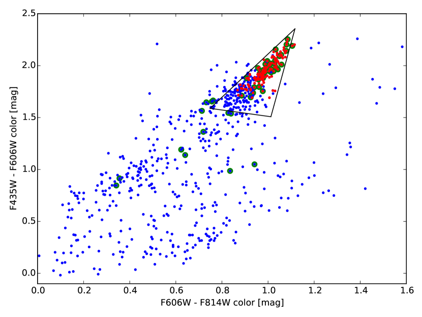
Individual galaxies are selected through a color cut, using the three optical HFF bands. In particular, we construct the F435W-F606W and F606W-F814W color-magnitude diagrams and look for evidence of a red-sequence. We then combine the two plots into a color-color diagram and select galaxies which fall into the tight cluster locus (Figure 7). To measure galaxy photometry, we run SExtractor (Bertin & Arnouts, 1996) in dual-image mode, using the F814W band data as the detection template. In the region covered by the MUSE footprint, we further refine the selection process by including all spectroscopically-confirmed cluster members and rejecting all non cluster members regardless of their colors. Additionally, we limit the selection to bright galaxies (), since beyond this cutoff – roughly equivalent to 0.02 – galaxies will have a negligible effect on the mass budget. We also exclude galaxies at distances beyond ″ from the cluster center ( , ), corresponding to kpc in physical space, for similar reasons.
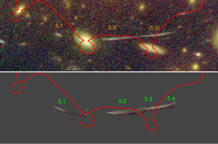
We constrain the mass model with the positions of known multiply-imaged systems, however, we first revise the interpretation of System 5, previously described as a 3-image system (5.1, 5.2, 5.3). Image 5.3 is actually located close to a background galaxy at (object B6 in Table 3) which perturbs the lens model, and we add it as an additional galaxy-scale potential. As illustrated by a simulation of the lensing effect on Images 5.1 and 5.2, this small perturbation convincingly produces a merging pair of two additional images previously identified as 5.3 (Figure 8.) Therefore, we update our constraint list to include the new Image 5.3 and Image 5.4 in the model. While we use nearly all of the 22 current systems (Table 1) we exclude System 10, a faint radial arc without a secure redshift that also lacks bright counterimages. Because even small changes in the mass model produce wildly different predictions for radial systems, the lack of counterimages makes the system fully degenerate with the parameters of the Northern cluster halo.
While some systems have only a single MUSE detection (Systems 16, 17, 18, 19, and 22), these objects are often bright in broadband photometry, and we are able to identify their counterparts in the HFF data directly. In fact, many lens systems with MUSE spectroscopy have at least one counterimage that falls outside of the current footprint, since the GTO data only cover a fraction of the A370 field of view. Though we are unable to confirm these objects spectroscopically, we can identify them with the help of the lens model itself. Specifically, we start with known (spectroscopically confirmed) members of a given lens system and use the model to predict the location of counterimages. From this rough guess, we look for candidates in the HFF data that match the system members (i.e., galaxies with similar colors, morphology, and shape), which we take to be the counterimages. We then optimize a new version of the model, including these other constraints. We can compare the models with and without the added constraints, and if the new results stay within an acceptable error limit: an average model rms displacement of 1″ or lower, we keep the counterimages and start the process again. In this way, we are able to iteratively refine and improve the model until it converges on the best solution.
In the best A370 model, we identify 16 counterimages this way: Images 7.4, 7.5, 14.4, 14.5, 15.4, 15.5, 16.3, 17.2, 17.3, 18.2, 18.3, 19.2, 19.3, 21.3, 22.2, and 22.3. With the exception of the System 7 counterimages, they are all associated with newly-identified MUSE objects, again highlighting the power of MUSE as a redshift engine. While the model also predicts the existence of Images 3.4 and 20.3, there are no obvious candidates in the available HFF data, so we do not include them as constraints. The remaining systems (8, 11, 12, and 13) fall outside of the MUSE footprint and lack secure redshift information. Thus, we use the positions of these systems as constraints but leave their redshift values as free parameters to be fit by the model. In some cases, the best-fit model predicts additional counterimages for these objects (Images 8.3, 11.3, and 13.3), but we again find no obvious counterparts in the HFF data, so we do not use them as model constraints. This is because predicted positions without redshift have significantly larger uncertainties. However, this will be revisited in future work with a larger MUSE mosaic. After adding and removing objects as described above, we are left with 21 unique systems with a total of 66 individual image constraints.
To optimize the model we feed all parameters and constraints into the LENSTOOL777https://projets.lam.fr/projects/lenstool/wiki (Kneib et al., 1996; Jullo et al., 2007; Jullo & Kneib, 2009) software program, which probes the full parameter space with a Bayesian Markov Chain Monte Carlo (MCMC) sampler. To evaluate a given model, LENSTOOL reconstructs the parametrized mass distribution and transforms the constraint coordinates from the image (observed) plane to the source (undeflected) plane. In the source plane, the program calculates the barycenter of each constraining system, then transforms these results back to the lens plane, creating a set of predicted images that can be compared to observation. By minimizing the rms displacement between prediction and observation, LENSTOOL is thus able to objectively determine the “best” model for a given set of input parameters (e.g., Kneib et al. 1996; Limousin et al. 2007a).
Following Richard et al. (2014), our initial model includes two massive cluster potentials (each centered on a BCG) and the cluster galaxies selected from the color-color cut outlined above. However, after several MCMC iterations with this model, we find that no combination of parameter values sufficiently recreates the observed image positions (i.e., with an average rms error 1″.) In particular, we are unable to simultaneously model the positions of the systems in the North and the new MUSE-identified images near the center. This is most noticeable in System 12, where typical model displacements can be as as large as 6″.
To help correct this disagreement, we first add an elongated, bar-like mass potential (DM3) as a bridge between the two cluster halos (Table 4). This flattens the mass distribution in the region between the two BCGs, and improves the fit of the central, radial image constraints of Systems 7, 14, and 15. As a consequence of adding the bar, the Northern cluster potential (DM2) becomes more elongated and its centroid moves further away from the BCG. This can be explained as a model degeneracy between the positions of DM2 and DM3, since there is a significant overlap between their mass distributions. In fact, the barycenter of the two components falls slightly to the South of the BCG itself.
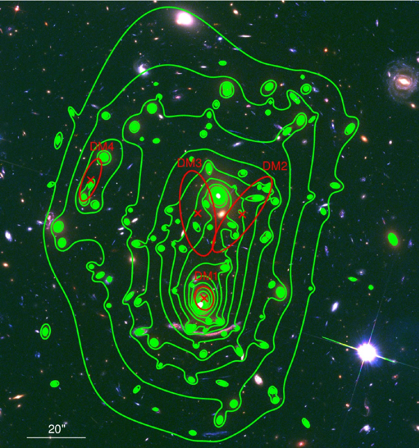
Even after adding the bar, however, we are only able to reduce the model rms to 1.17″, with the Northern systems still poorly fit. Therefore, we add an additional large-scale cluster potential to the model (DM4), centered near a group of bright galaxies in the northeastern corner of the cluster (see Figure 9). This location is chosen both because of its proximity to Image 12.3 (the image constraint with the highest rms error), and because it is part of a “crown” of galaxies sitting above the northern BCG. Since all of the galaxies in the crown are bright and have similar, cluster-like colors and several are spectroscopically confirmed to be cluster members (Mellier et al., 1988) it is possible this collection represents another, unaccounted-for mass component of A370.
As with the other cluster potentials, we allow the dPIE parameters of the crown component to vary freely within a set of priors, though we assume an initial configuration that is more elliptical (like the bar), to better account for the stretched nature of the crown. Including this additional mass clump further improves the fit, reducing the average rms displacement from 1.17″ to 0.94″, below the benchmark level of rms = 1″.
To see if even more mass structures are needed to describe A370, we also test a 5-clump mass model, placing an additional mass clump on the Western side of the A370 crown. However, this does not significantly improve the fit (rms = 0.88″) and actually lowers the Bayesian evidence, possibly suggesting an overfit to the data (see Section 5.1.) Thus, given the success of the 4-clump model in reproducing the image constraint positions, we treat its optimized parameter set as our “best-fit”description of the A370 mass distribution. Optimized parameters for all models can be seen in Table 4, and the final model mass reconstruction is shown in Figure 9.
| Model Name | Component | |||||||
|---|---|---|---|---|---|---|---|---|
| (Fit Statistics) | (″) | (″) | () | (kpc) | (kpc) | (km s-1) | ||
| 2-Clump | DM1 | |||||||
| rms = 2.81″ | DM2 | |||||||
| = 31.97 | BCG1 | |||||||
| () = -1652.47 | BCG2 | |||||||
| () = -1817.07 | CL32 | |||||||
| BIC = 3404.75 | L∗ galaxy | – | – | – | – | |||
| 3-Clump | DM1 | |||||||
| rms = 1.17″ | DM2 | |||||||
| = 6.00 | DM3 | |||||||
| () = -209.75 | BCG1 | |||||||
| () = -303.19 | BCG2 | |||||||
| BIC = 554.49 | CL32 | |||||||
| Galaxy | – | – | – | – | ||||
| 4-Clump | DM1 | |||||||
| rms = 0.94″ | DM2 | |||||||
| = 4.33 | DM3 | |||||||
| () = -146.48 | DM4 | |||||||
| () = -201.90 | BCG1 | |||||||
| BIC = 455.35 | BCG2 | |||||||
| CL32 | ||||||||
| Galaxy | – | – | – | – | ||||
| 5-Clump | DM1 | |||||||
| rms = 0.88″ | DM2 | |||||||
| = 4.29 | DM3 | |||||||
| () = -133.64 | DM4 | |||||||
| () = -202.67 | DM5 | |||||||
| BIC = 456.27 | BCG1 | |||||||
| BCG2 | ||||||||
| CL32 | ||||||||
| Galaxy | – | – | – | – |
a and are measured relative to the reference coordinate point: ( = 39.97134, = -1.5822597)
b Ellipticity () is defined to be , where and are the semi-major and semi-minor axes of the ellipse
c Quantities in brackets are fixed parameters
5 Discussion
5.1 The Case for Additional Mass Clumps
While adding two new large-scale mass clumps to the model significantly improves the fit, it is important to ask the question “Is this additional mass truly necessary?” In other words, are these new mass clumps real features supported by the data, or is it simply a case of overfitting in a sparsely sampled region of the cluster? To answer this, we look at both model and (perhaps more importantly) physical evidence.
From a purely statistical point of view, the Bayesian evidence value () can discriminate between models, taking into account and in some cases penalizing additional terms and model complexities, while simultaneously evaluating goodness of fit. Models with larger evidence terms are preferred over those with smaller terms, providing an objective criterion for comparison (see e.g., Limousin et al. 2010). For the A370 models (Table 4), we find that the evidence of the 3-clump model ( = -303.19) is significantly larger than that of the 2-clump model ( = -1817.07), showing that the data strongly prefer a mass distribution that includes a flatter, central “bar” component. The evidence term of the 4-clump model is larger still ( = -201.90) – though the relative improvement over the 3-clump model is not as great – again suggesting a real need for the crown clump. Finally, although the more complex 5-clump model has a marginally improved fit over the 4-clump model (rms = 0.88″), its evidence value actually decreases ( = -202.67) suggesting that the fifth mass clump is unnecessary and that we are beginning to overfit the system. Additional tests, placing the fifth clump at several other locations throughout the crown, yield similar (or worse) results.
As a complementary check on overfitting, we also calculate the Bayesian information criterion (BIC) term for each model:
| (1) |
where is the model likelihood, is the number of model free parameters, and is the number of model constraints. Lower BIC values are favored over higher values, and for our models, we again see that the 4-clump case (BIC = 455.35) is preferred over all others (we present all values in Table 4), bolstering the claim that the bar and the crown are real, necessary features.
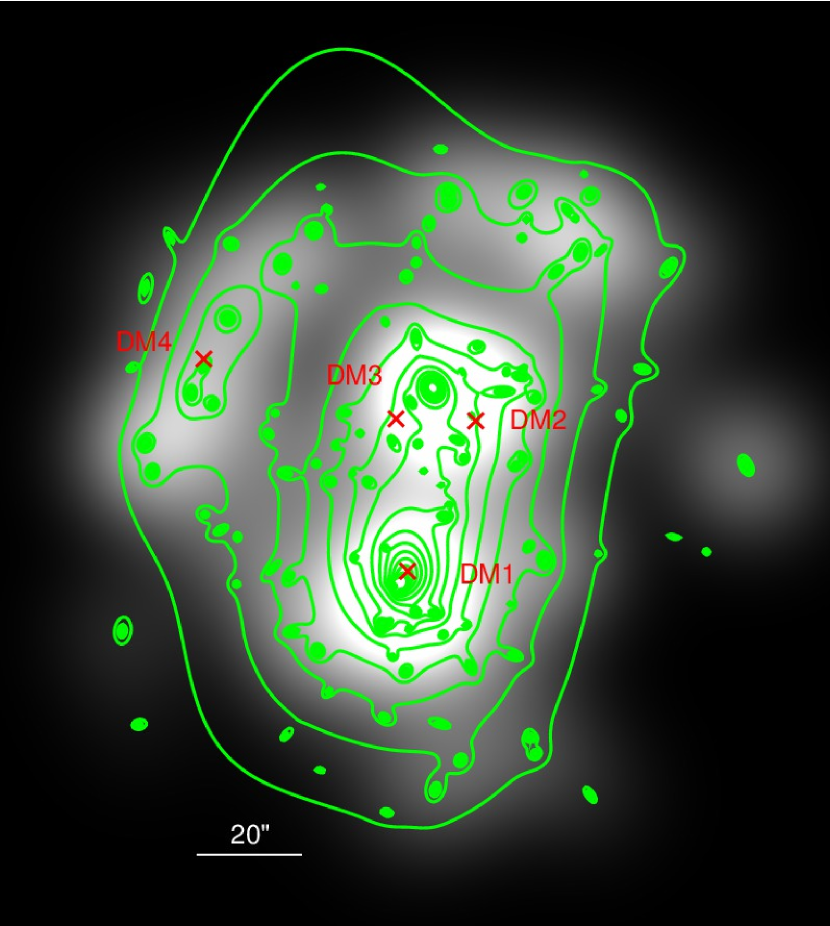
On the physical side of the evidence argument, we first turn to the cluster light distribution. As previously mentioned, the presence of the Northern crown of galaxies already suggests an additional mass distribution not captured by the two-clump model. To test this theory, we first isolate the cluster light in the F814W band (the filter where cluster members are brightest), keeping only the objects selected by the cluster-member color-color cut (Section 4) and masking the rest. We then smooth the remaining light with a Gaussian kernel (″), providing a cleaner view of the light distribution. Comparing this distribution to the 4-clump mass model (Figure 10, left), we find good agreement between the brightest points of the light map and the positions of the large-scale clumps. As expected, the Southern cluster halo sits near the southern BCG, the combined Northern cluster halo and bar surround the Northern BCG, and the fourth clump sits on the Eastern side of the crown. Even more promisingly, the orientation of the fourth mass clump is aligned with the distribution of the crown light, even though it is allowed to vary freely in the model. Assuming then that, at least to some degree, the presence of light traces the presence of mass, the agreement between the light map and mass model provides another argument in favor of the 4-clump model.
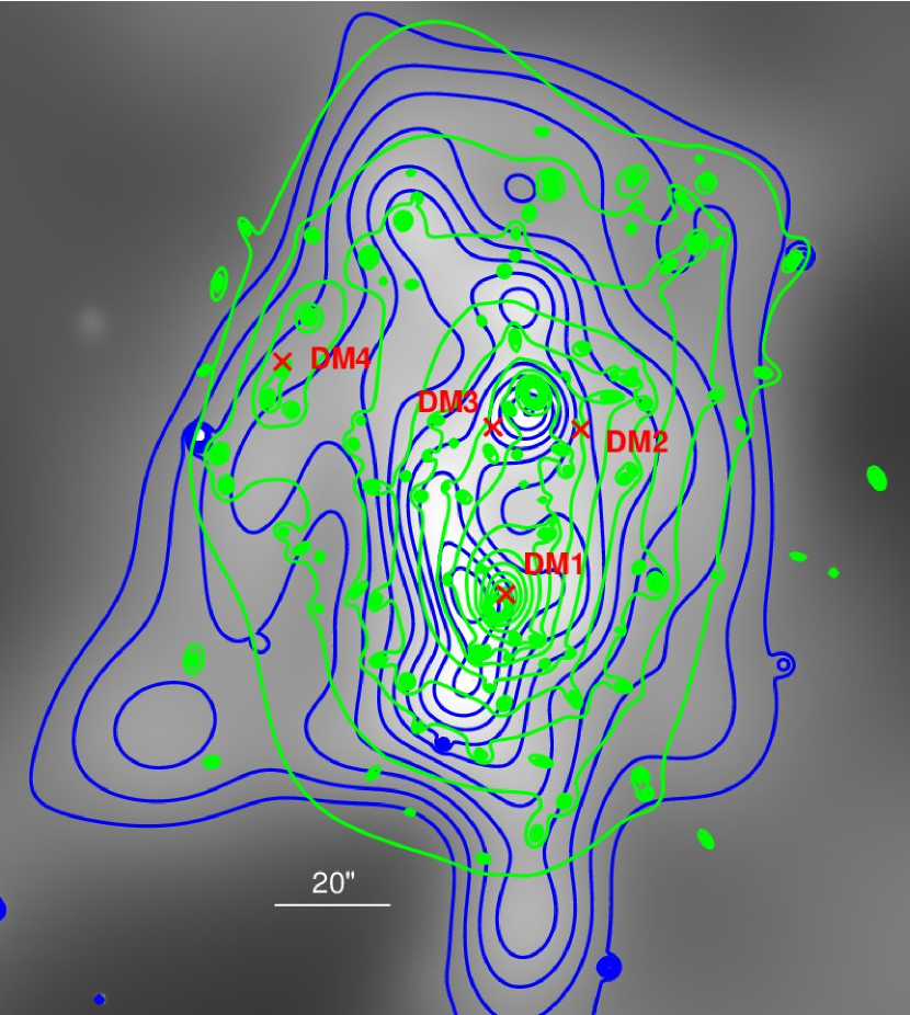
Finally, we also look at the A370 X-ray gas profile, as the presence of hot X-ray gas is often used as a tracer of deep mass potentials. For this, we turn to publicly available, deep Chandra data: an 88 ks image of A370, observed using the using the Advanced CCD Imaging Spectrometer S-array (ACIS-S) camera (ID: 08700025, PI: G. Garmire). After smoothing the X-ray map using the ASMOOTH algorithm (Ebeling, White, & Rangarajan, 2006), we compare the smoothed X-ray map to the positions of the 4-clump mass model components (Figure 10, right). While the results here are not as definitive as in the cluster-light case, we do still see a moderate agreement between the map and the clump positions. Generally, the X-ray contours are also slightly extended in the vicinity of the crown clump, again hinting at the presence of an additional potential well.
Focusing more closely on the X-ray contours, we can see that they follow a distinct box-like pattern, which is especially noticeable in the outskirts of the cluster. Interestingly, the mass contours in the 4-clump model have a similar shape, largely driven by the overlap between the Northern cluster halo and the central bar. Given the rough agreement between the X-ray and mass contours, it is possible that the best-fit positions of the Northern mass clumps are more than a simple degeneracy, but instead driven by physical parameters.
Thus, taken as a whole, the combination of physical and statistical evidence indicate that the additional mass clumps in the cluster center and crown region are necessary components of the mass model. This suggests an even more complex mass distribution than previously thought, motivating future studies in this area.
5.2 Comparisons with Other Models
Thanks to the discovery of several new lensing constraints, our picture of the A370 mass distribution is beginning to evolve. While the addition of new mass clumps is the largest change, it is not the only difference. To get a better understanding of these changes and what they mean physically, we can compare our model to previous results. This is especially easy with the models presented by Johnson et al. (2014) and Richard et al. (2014), since they were both also generated with LENSTOOL, using a similar set of parameters. On the whole, while the total mass of A370 remains largely unchanged between models, where the mass enclosed within a 500 kpc circular radius is in each case, the distribution of mass between various components does not. In particular, we find that the cluster halo associated with the Southern BCG (DM1) is much rounder and more compact than either of the previous models, flattening the mass profile in this region. This is predominantly due to the number of radial, 5-image systems seen near the Southern cluster (Systems 7, 14, and 15), as a more elliptical mass distribution would break the symmetry and destroy the radial arcs. Conversely, the Northern cluster halo (DM2) is more elliptical and tilted at a steeper angle away from North, though this is largely caused by an interaction with the central bar component. Both cluster potentials are also considerably less massive in our model, which is another consequence of the bar. Finally, we note that our model favors a significantly larger galaxy velocity dispersion, placing more emphasis on localized substructure contributions to the total mass profile. A list of specific parameter differences can be seen in Table 5.
| Parameter | Modela | |||||
| (km s-1) | (degree) | (kpc) | (kpc) | |||
| DM1 | J14 | 969 | 0.47 | 80.8 | 88.2 | [1500]b |
| R14 | 833 | 0.59 | -106.0 | 64.0 | [1000] | |
| L16 | ||||||
| DM2 | J14 | 1040 | 0.09 | 89.4 | 94.7 | [1500] |
| R14 | 1128 | 0.38 | -89.6 | 155.0 | [1000] | |
| L16 | ||||||
| Galaxy | J14 | [120] | — | — | [0.15] | [120] |
| R14 | 116 | — | — | [0.15] | 61.0 | |
| L16 | — | — |
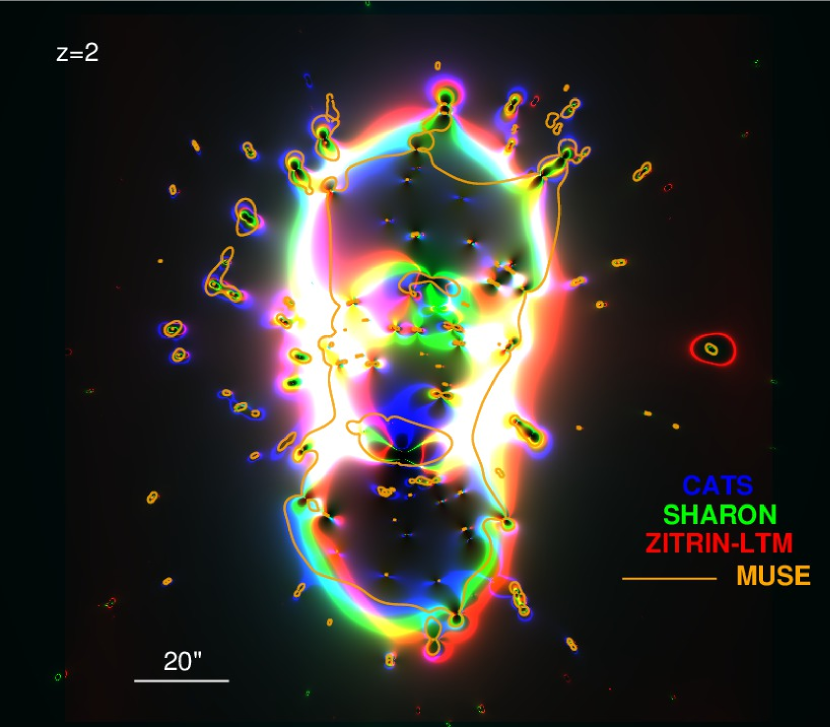
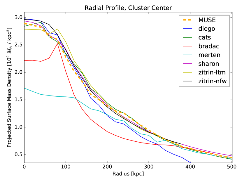
In addition to specific model parameters, we can also compare the total mass properties of our model. For this exercise, we turn to the public models constructed for the HFF lens modeling initiative. In the left panel of Figure 11, we show the critical curve for our best-fit model, compared to the magnification maps of three different HFF models: “CATS”, from the Clusters As TelescopeS team, (Co-PIs: J.P. Kneib and P. Natarajan), “Sharon v.2” (PI, K. Sharon), and “Zitrin-LTM” (PI, A. Zitrin). We select these models because they are constructed using only strong-lensing constraints, and because the resolution of their magnification maps at the core of the cluster is sufficiently high enough to compare their critical curves. In general, the shape of our curve largely traces the high-magnification regions in the other models, suggesting a broad agreement between our work and earlier studies. However, we do note that our curve has a boxier shape, due to the interaction between the Northern cluster halo and the central bar and to the presence of the crown clump. Furthermore, the radial critical region (traced out by the internal orange line) is much larger in our model. This is again a result of the rounder, flatter mass distribution predicted by our model, and also highlights the increased area containing radial lensing constraints such as Systems 7, 14, and 15.
These features can also be seen in the right-hand panel of Figure 11, where we show the radial surface mass density profile for several models (including Diego et al. 2016), starting from a point roughly centered between the two BCGs ( , ). At small radii ( 100 kpc), our mass profile is lower than several others, since this region covers the flatter core responsible for the extended radial critical curve. On the other hand, our model profile is slightly higher than the others between 200 and 300 kpc, due to the crown mass clump.
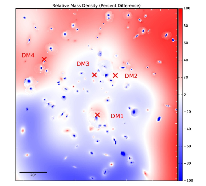
Of course, important spatial information is lost when the mass map is radially averaged, so it is important to look for differences in the full 2D mass distribution, as well. For this test, we compare our 4-clump model to the free-form model presented in Diego et al. (2016), which is also generated from HFF data, but constructed in a completely independent way, reducing potential sources of unknown bias. To make the comparison, we subtract the free-form model’s mass density map from our own map, measuring relative differences on a pixel-by-pixel basis. The results can be seen in Figure 12. Overall, we do see differences between the two approaches: The Diego et al. (2016) model is generally more concentrated and slightly rounder. Our parametric approach shows a noticeable overdensity in the vicinity of the crown, due to the crown mass clump (DM4) in the East, and the extension of the Northern cluster clump and the central bar (DM2 and DM3, respectively) in the Northwest. The parametric model also has a larger fraction of total mass in the outskirts of the cluster, which is also seen in the radial profile presented in Figure 11. While model differences can be large at large radii – the parametric model is rougly twice as dense as the free-form model at the edges of the map – we note that the absolute mass density values at these distances are very small ( kpc-2) and contribute a negligible amount to the total mass budget. Conversely, the relative differences near the cluster center are typically less than 10 percent, resulting in an overall good agreement between the two models.
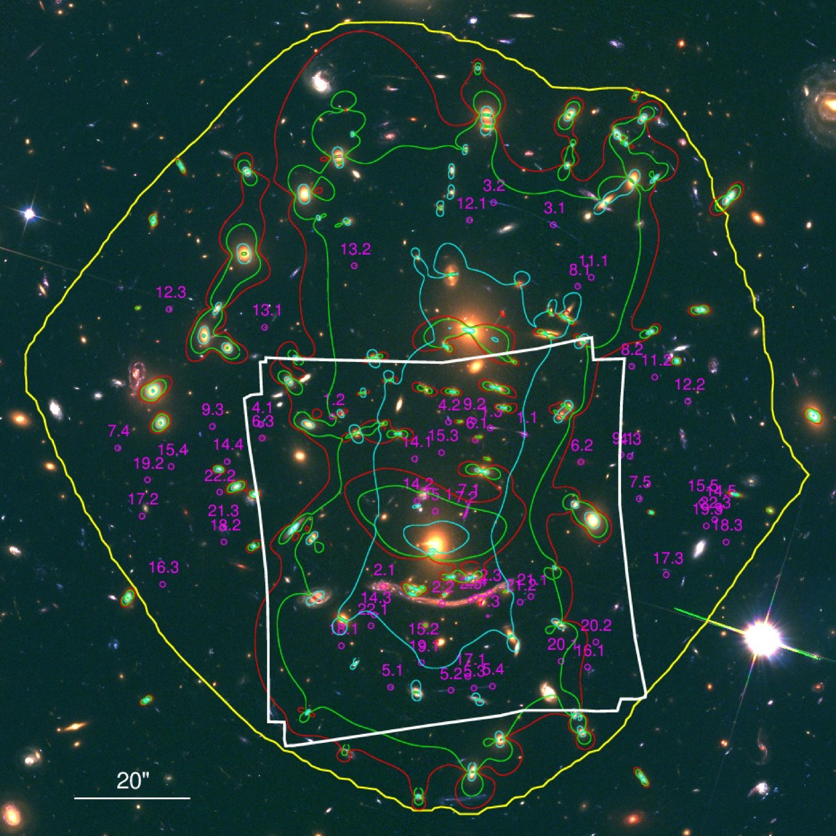
Finally, we can compare our model (and all models) of A370 to other clusters in the HFF program. The combined rms error for our best fit model ( = 0.94″) is higher than the error presented in Johnson et al. (2014) ( = 0.82″), comparable to the error in Richard et al. (2014) ( = 0.93″), and smaller than the error presented in Richard et al. (2010) ( = 1.76″). However all of these rms values are larger than the best fit models of most other HFF clusters, such as MACS 0416 ( = 0.5″; Caminha et al. 2016) or Abell 2744 ( = 0.7″; Jauzac et al. 2016). Instead, while not as large, our rms is more similar to MACS 0717 ( = 1.9″; Limousin et al. 2016). Like MACS 0717, A370 is a complex cluster, with several interacting mass components covering a large field of view. In fact, the A370 “multiple-image zone” (Figure 13), the region predicted to contain all multiple images out to high redshift (), is the second largest of all of the Frontier Fields, behind only MACS 0717. Given the similarities, it is therefore unsurprising that the typical rms is also high.
To reduce the total rms further, we need to explore the other areas of the cluster with MUSE. This will help to refine the model even more and allow us to test whether or not our current interpretation is correct. In particular, the crown mass clump may only be a temporary solution; future data may require additional large-scale halos, or even suggest an alternative to the crown. We cannot be sure of this until we have additional constraints in the North. Fortunately, such a survey is currently underway (PI F. Bauer), and the results of this study will be the topic of a future paper.
6 Conclusions
In this paper, we have presented a new mass model for the A370 cluster, taking advantage of deep HFF imaging and new MUSE spectroscopy. Our main conclusions are as follows:
-
•
We present a MUSE-based redshift catalog for A370, consisting of 120 secure redshifts (), including 34 multiply-imaged background objects (comprising 15 unique systems), 13 singly-imaged background galaxies, 56 cluster members, 13 foreground galaxies, and 4 stars.
-
•
Together, HFF and MUSE data are a powerful combination, greatly improving our ability to construct lens models. MUSE spectroscopy is particularly valuable for this work, as it can be used to blindly identify new lensing constraints without selecting a specific redshift range.
-
•
After constructing a mass model with the new multiply-imaged constraints, we find two key differences with previous work:
1.) A central core that is flatter and less massive due to an increase in radial lensing systems
2.) The need for additional large-scale mass clumps (“the bar” and “the crown”) to better fit lensing constraints in the North of the cluster
-
•
A lack of model constraints in the North makes accurate comparisons difficult. We will need more MUSE data, covering a larger area of the A370 cluster to discriminate between possible interpretations. These data are currently being taken, and will be the subject of an upcoming paper.
Additionally, our model can be used as a guide for upcoming observations, as high-magnification regions in our models (Figure 13) should be ideal places to look for new, magnified high-redshift galaxies. With new MUSE spectroscopy on the way, the A370 cluster should continue to provide a wealth of new information in the future.
Acknowledgments
DJL, JR, BC, GM, VP and JM acknowledge support from the ERC starting grant CALENDS. This work has been carried out thanks to the support of the ANR FOGHAR (ANR-13-BS05-0010-02) and the OCEVU Labex (ANR- 11-LABX-0060). LW acknowledges support by the Competitive Fund of the Leibniz Association through grant SAW-2015-AIP-2.
References
- Abell (1958) Abell G. O., 1958, ApJS, 3, 211
- Bacon et al. (2010) Bacon R., et al., 2010, SPIE, 7735, 773508
- Bacon et al. (2015) Bacon R., et al., 2015, A&A, 575, A75
- Baldry et al. (2014) Baldry I. K., et al., 2014, MNRAS, 441, 2440
- Bernardi et al. (2003) Bernardi M., et al., 2003, AJ, 125, 1849
- Bertin (2006) Bertin E., 2006, ASPC, 351, 112
- Bertin & Arnouts (1996) Bertin E., Arnouts S., 1996, A&AS, 117, 393
- Bézecourt et al. (1999a) Bézecourt J., Kneib J. P., Soucail G., Ebbels T. M. D., 1999a, A&A, 347, 21
- Bézecourt et al. (1999b) Bézecourt J., Soucail G., Ellis R. S., Kneib J.-P., 1999b, A&A, 351, 433
- Bina et al. (2016) Bina D., et al., 2016, A&A, 590, A14
- Bradač et al. (2008a) Bradač M., et al., 2008a, ApJ, 681, 187-196
- Bradač et al. (2008b) Bradač M., Allen S. W., Treu T., Ebeling H., Massey R., Morris R. G., von der Linden A., Applegate D., 2008b, ApJ, 687, 959-967
- Caminha et al. (2016) Caminha G. B., et al., 2016, arXiv, arXiv:1607.03462
- Diego et al. (2016) Diego J. M., et al., 2016, arXiv, arXiv:1609.04822
- Ebeling, Edge, & Henry (2001) Ebeling H., Edge A. C., Henry J. P., 2001, ApJ, 553, 668
- Ebeling, White, & Rangarajan (2006) Ebeling H., White D. A., Rangarajan F. V. N., 2006, MNRAS, 368, 65
- Ebeling et al. (2009) Ebeling H., Ma C. J., Kneib J.-P., Jullo E., Courtney N. J. D., Barrett E., Edge A. C., Le Borgne J.-F., 2009, MNRAS, 395, 1213
- Elíasdóttir et al. (2007) Elíasdóttir Á., et al., 2007, arXiv, arXiv:0710.5636
- Ford et al. (2003) Ford H. C., et al., 2003, SPIE, 4854, 81
- Fort et al. (1988) Fort B., Prieur J. L., Mathez G., Mellier Y., Soucail G., 1988, A&A, 200, L17
- Halkola, Seitz, & Pannella (2007) Halkola A., Seitz S., Pannella M., 2007, ApJ, 656, 739
- Hoag et al. (2016) Hoag A., et al., 2016, arXiv, arXiv:1603.00505
- Hsu, Ebeling, & Richard (2013) Hsu L.-Y., Ebeling H., Richard J., 2013, MNRAS, 429, 833
- Jauzac et al. (2014) Jauzac M., et al., 2014, MNRAS, 443, 1549
- Jauzac et al. (2015) Jauzac M., et al., 2015, MNRAS, 452, 1437
- Jauzac et al. (2016) Jauzac M., et al., 2016, MNRAS, 457, 2029
- Johnson et al. (2014) Johnson T. L., Sharon K., Bayliss M. B., Gladders M. D., Coe D., Ebeling H., 2014, ApJ, 797, 48
- Jullo & Kneib (2009) Jullo E., Kneib J.-P., 2009, MNRAS, 395, 1319
- Jullo et al. (2007) Jullo E., Kneib J.-P., Limousin M., Elíasdóttir Á., Marshall P. J., Verdugo T., 2007, NJPh, 9, 447
- Karman et al. (2015) Karman W., et al., 2015, A&A, 574, A11
- Kawamata et al. (2016) Kawamata R., Oguri M., Ishigaki M., Shimasaku K., Ouchi M., 2016, ApJ, 819, 114
- Kimble et al. (2008) Kimble R. A., MacKenty J. W., O’Connell R. W., Townsend J. A., 2008, SPIE, 7010, 70101E
- Kneib et al. (1996) Kneib J.-P., Ellis R. S., Smail I., Couch W. J., Sharples R. M., 1996, ApJ, 471, 643
- Kneib et al. (1993) Kneib J. P., Mellier Y., Fort B., Mathez G., 1993, A&A, 273, 367
- Limousin et al. (2007a) Limousin M., et al., 2007a, ApJ, 668, 643
- Limousin et al. (2007b) Limousin M., Kneib J. P., Bardeau S., Natarajan P., Czoske O., Smail I., Ebeling H., Smith G. P., 2007b, A&A, 461, 881
- Limousin et al. (2010) Limousin M., et al., 2010, A&A, 524, A95
- Limousin et al. (2016) Limousin M., et al., 2016, A&A, 588, A99
- Lotz et al. (2016) Lotz J. M., et al., 2016, arXiv, arXiv:1605.06567
- Lynds & Petrosian (1986) Lynds R., Petrosian V., 1986, BAAS, 18, 1014
- Lynds & Petrosian (1989) Lynds R., Petrosian V., 1989, ApJ, 336, 1
- Massey et al. (2015) Massey R., et al., 2015, MNRAS, 449, 3393
- Medezinski et al. (2011) Medezinski E., Broadhurst T., Umetsu K., Benítez N., Taylor A., 2011, MNRAS, 414, 1840
- Mellier et al. (1988) Mellier Y., Soucail G., Fort B., Mathez G., 1988, A&A, 199, 13
- Mellier et al. (1991) Mellier Y., Fort B., Soucail G., Mathez G., Cailloux M., 1991, ApJ, 380, 334
- Monna et al. (2014) Monna A., et al., 2014, MNRAS, 438, 1417
- Morandi, Ettori, & Moscardini (2007) Morandi A., Ettori S., Moscardini L., 2007, MNRAS, 379, 518
- Natarajan et al. (2009) Natarajan P., Kneib J.-P., Smail I., Treu T., Ellis R., Moran S., Limousin M., Czoske O., 2009, ApJ, 693, 970
- Oguri (2010) Oguri M., 2010, PASJ, 62, 1017
- Patrício et al. (2016) Patrício V., et al., 2016, MNRAS, 456, 4191
- Postman et al. (2012) Postman M., et al., 2012, ApJS, 199, 25
- Richard et al. (2010) Richard J., Kneib J.-P., Limousin M., Edge A., Jullo E., 2010, MNRAS, 402, L44
- Richard et al. (2014) Richard J., et al., 2014, MNRAS, 444, 268
- Richard et al. (2015) Richard J., et al., 2015, MNRAS, 446, L16
- Rosati et al. (2014) Rosati P., et al., 2014, Msngr, 158, 48
- Schmidt et al. (2014) Schmidt K. B., et al., 2014, ApJ, 782, L36
- Sharon et al. (2012) Sharon K., Gladders M. D., Rigby J. R., Wuyts E., Koester B. P., Bayliss M. B., Barrientos L. F., 2012, ApJ, 746, 161
- Smail et al. (1996) Smail I., Dressler A., Kneib J.-P., Ellis R. S., Couch W. J., Sharples R. M., Oemler A., Jr., 1996, ApJ, 469, 508
- Soto et al. (2016) Soto K. T., Lilly S. J., Bacon R., Richard J., Conseil S., 2016, MNRAS, 458, 3210
- Soucail et al. (1987) Soucail G., Fort B., Mellier Y., Picat J. P., 1987, A&A, 172, L14
- Soucail et al. (1988) Soucail G., Mellier Y., Fort B., Mathez G., Cailloux M., 1988, A&A, 191, L19
- Treu et al. (2015) Treu T., et al., 2015, ApJ, 812, 114
- Umetsu et al. (2011) Umetsu K., Broadhurst T., Zitrin A., Medezinski E., Hsu L.-Y., 2011, ApJ, 729, 127
- Weilbacher et al. (2012) Weilbacher P. M., Streicher O., Urrutia T., Jarno A., Pécontal-Rousset A., Bacon R., Böhm P., 2012, SPIE, 8451, 84510B
- Weilbacher et al. (2014) Weilbacher P. M., Streicher O., Urrutia T., Pécontal-Rousset A., Jarno A., Bacon R., 2014, ASPC, 485, 451
- Zitrin et al. (2011) Zitrin A., et al., 2011, ApJ, 742, 117