Optimal Oil Production under Mean Reverting Lévy Models with Regime Switching

Abstract

This paper is concerned with the problem of finding the optimal of extraction policies of an oil field in light of various financial and economical restrictions and constraints. Taking into account the fact that the oil price in worldwide commodity markets fluctuates randomly following global and seasonal macro-economic parameters, we model the evolution of the oil price as a mean reverting regime switching jump diffusion process. We formulate this problem as finite-time horizon optimal control problem. We solve the control problem using the method of viscosity solutions. Moreover, we construct and prove the convergence of a numerical scheme for approximating the optimal reward function and the optimal extraction policy. A numerical example that illustrates these results is presented.

Keywords: Oil Production, Jump Diffusion, Regime Switching, Equilibrium Price of Oil, Finite Difference Approximations.

1 Introduction

Oil and natural gas have always been the main sources of revenue for a large number of developing countries as well as some industrialized nations around the world. Oil extraction policies vary from a country to another, in some countries the extraction is done by a state owned corporation in others it is done by foreign multinationals. The production and regulation of strategic natural resources such as oil, natural gas, uranium, gold, copper,…,etc have always been among of the leading topics in geopolitical and macro-economical debates between politicians as well as financial economists in academic circles.
The optimal extraction of natural resources was first studied done by Hotelling (1931), he derived an optimal extraction policy under the assumption that the commodity price is constant. Many economists have extended the Hotelling model by taking into account the uncertainty in the supply, the demand, as well as the ever-changing regulatory landscape of natural resource policies. Among many others, one can cite the work of Sweeney (1977), Hanson (1980), Solow and Wan (1976), Pindyck (1978), (1980), Lin and Wagner (2007) for various extensions of the basic Hotelling model. Cherian et al. (1998) studied the optimal extraction of nonrenewable resources as a stochastic optimal control problem with two state variables, the commodity price and the size of the remaining reserve. They solved the control problem numerically by using Markov chain approximation methods developed by Kushner (1977) and Kushner and Dupuis (1992). Recently Aleksandrov et al. (2012) studied the optimal production of oil as an American-style real option and used Monte-Carlo methods to approximate the optimal production rate when the oil price follows a mean-reverting process.
It is also self evident that the price of oil in commodity exchange markets fluctuates following divers macro economical and global geopolitical forces. It is therefore crucial to take into account the random dynamic of the commodity value when solving the optimal extraction problem in order to maintain the validity of the result obtained. In this paper, we use the mean reverting regime switching Lévy processes to model the oil price. Mean reverting processes were first used to describe the evolution of commodity prices by Gibson an Schwartz (1990) and Schwartz (1997), these processes capture perfectly the mean reversion feature of commodity prices around an equilibrium price when the market is stable. Other authors like Schwartz and Smith (2000) and Aleksandrov et al. (2012) used the mean reverting processes in their extraction models. Oil prices also display a great deal of seasonality, jumps and spikes due to various supply disruptions and political turmoils in oil-rich countries, we use regime switching jump diffusions to capture all those effects. Thus our pricing model closely captures the instability of oil markets. Regime switching models have been extensively used in the financial economics literature since its introduction by Hamilton (1989). Many authors have studied the control of systems that involve regime switching using a hidden Markov chain, one can cite Zhang and Yin (1998), (2005), Pemy and Zhang (2006), Pemy (2011), (2014) among others.
In this paper we treat the problem of finding optimal extraction strategies as an optimal control problem of a mean reverting Markov switching Lévy processes in a finite time horizon. The main contribution of this paper is two-fold, first we prove that the value function is the unique viscosity solution of the associated Hamilton-Jacobi-Bellman equation. Then, we build a finite difference approximation scheme and prove its convergence to the unique viscosity solution of HJB equation. This enable us to derive both the optimal reward function and the optimal extraction policy in this broad setting.
The paper is organized as follows. In the next section, we formulate the problem under consideration. In section 3 we derive the properties of the value function and characterize it as unique viscosity solution of the Hamilton Jacobi Bellman equation. And in section 4, we construct a finite difference approximation scheme and prove its convergence to the value function. Finally, in section 5, we give a numerical example.

2 Problem formulation

Consider a multinational oil company with an extraction lease that expires in $T$ years, $0<T<\infty$. We assume that the market value of a barrel of oil at time $t$ is $S_{t}=e^{X_{t}}$. Given that oil prices are very sensitive global macro-economical and geopolitical shocks, we model $X_{t}$ as a mean reverting regime switching Lévy process with two states. Let $\alpha(t)\in{\cal M}=\{1,2\}$ be a finite state Markov chain that captures the state of the oil market: $\alpha(t)=1$ indicates the bull market at time $t$ and $\alpha(t)=2$ represents a bear market at time $t$. The generator of this Markov chain is

$$\begin{array}[]{rl}Q=\left(\begin{array}[]{ll}-\lambda_{1}&\lambda_{1}\\ \lambda_{2}&-\lambda_{2}\end{array}\right),\qquad\lambda_{1}>0,\lambda_{2}>0.\end{array}$$

Let $(\eta_{t})_{t}$ be a Lévy process and let $N$ be the Poisson random measure of $(\eta_{t})_{t}$, $N(t,U)=\sum_{0<s\leq t}{\bf 1}_{U}(\eta_{s}-\eta_{s^{-}})$ for any Borel set $U\subset{\mathbb{R}}$. Moreover, let $\nu$ be the Lévy measure of $(\eta_{t})_{t}$ we have $\nu(U)=E[N(1,U)]$ for any Borel set $U\subset{\mathbb{R}}$. The differential form of $N$ is denoted by $N(dt,dz)$, we define the differential $\bar{N}(dt,dz)$ as follows

$$\begin{array}[]{rl}\displaystyle\bar{N}(dt,dz)=\left\{\begin{array}[]{ll}N(dt,dz)-\nu(dz)dt&\hbox{if }|z|<1\\ N(dt,dz)&\hbox{if }|z|\geq 1.\end{array}\right.\end{array}$$

We assume that the Lévy measure $\nu$ has finite intensity,

$$\displaystyle\Gamma=\int_{{\mathbb{R}}}\nu(dz)<\infty.$$ (1)

In other terms, the total sum of jumps and spikes of the oil price during the lifetime of the contract is finite. Let $K<\infty$ be the total size of the oil field at the beginning of the lease, and let $Y(t)$ be the size of the remaining reserve of the oil field by time $t$, obviously $Y(t)\in[0,K]$. The state variables of our control problem are $X(t)\in{\mathbb{R}}$ and $Y(t)\in[0,K]$, and the state space is $[0,\infty)\times[0,K]$. We assume that the processes $X(t),Y(t)$ follow the dynamics

$$\left\{\begin{array}[]{ll}\displaystyle\mathrm{d}X(t)&\displaystyle=\kappa\big{(}\mu(\alpha(t))-X(t)\big{)}\mathrm{d}t+\sigma(\alpha(t))\mathrm{d}W(t)+\int_{{\mathbb{R}}}\gamma(\alpha(t))z\bar{N}(dt,dz),\\ dY(t)&=-u(t)dt,\\ \displaystyle X(s)&=x\geq 0,\,\,\,\,Y(s)=y\geq 0,\qquad 0\leq s\leq t\leq T,\end{array}\right.$$ (5)

where $u(t)\in U=[0,\bar{u}]$ is the extraction rate chosen by the company. In fact the process $u(t)$ is control variable. The process $W(t)$ is the Wiener process defined on a probability space $(\Omega,{\cal F},P)$. Moreover, we assume that $W(t)$, $\alpha(t)$ and $\eta_{t}$ are independent. The parameter $\mu(\cdot)$ represents the equilibrium price of oil. For each state $i\in\{1,2\}$ of the oil market we assume that the corresponding equilibrium price $\mu(i)$ is known. Similarly $\sigma(\cdot)$ represents the volatility and $\gamma(\cdot)$ represents the intensity of the jump diffusion. For each state $i\in\{1,2\}$ of the oil market we assume that $\sigma(i),\,\gamma(i)$ are known constants. As a matter of fact $\gamma(i)$ captures the frequencies and sizes of jumps and spikes of the oil price. It is well known that the spot prices of energy commodities that are very expensive to store usually have frequent jumps and spikes within short periods of time. In order to capture those effects jump diffusions are the ideal candidates.

Definition 2.1.

The extraction rate $u(\cdot)$ taking values on intervals $[0,\bar{u}]$ is called an admissible control with respect to the initial data $(s,x,y,i)\in[0,T]\times[0,\infty)\times[0,K]\times{\cal M}$ if:

• Equation (5) has a unique solution with $X(s)=x$, $Y(s)=y$, $\alpha(s)=i$, and $X(t)\in[0,\infty),\,\,Y(t)\in[0,K]$ for all $t\in[0,T]$.

• The process $u(\cdot)$ is $\{{\cal F}_{t}\}_{t\geq 0}$-adapted where ${\cal F}_{t}=\sigma\{\alpha(s),W(s),\eta_{s};s\leq t\}$.

We use ${\cal U}={\cal U}(s,x,y,i)$ to denote the set of admissible controls taking values in $U=[0,\bar{u}]$ such that $X(s)=x$, $Y(s)=y$, $\alpha(s)=i$.

The admissibility condition implies that we should only consider extraction rates that depend on the information available up to time $t$, and within a reasonable range sets forth at the beginning of the lease and that will guarantee that the state variables stay in state space during the lifetime of the lease. We assume that the extraction cost function per unit of time $t$ is the function $C(t,Y(t),u(t))$ that depends on the extraction rate $u(t)$ and the size of the remaining reserve $Y(t)$. Moreover, $C(t,y,u)$ should be measurable and nondecreasing with respect to size of the remaining reserve $y$. This enables us to capture the fact that is more expensive to extract as the size of the oil field decreases. A typical example of an extraction cost function is

$$\begin{array}[]{rl}\displaystyle C(t,y,u)=a+mu(bY+c),\end{array}$$

where $a>0$ can be seen as the initial cost of setting up the mine and $m$, $b$, and $c$ are constants such that $m>0$ and $b,c\geq 0$. The total profit rate for operating the mine is

$$\begin{array}[]{rl}L(t,X(t),Y(t),u(t))=e^{X(t)}u(t)-C(t,Y(t),u(t))\quad t\in[0,T).\end{array}$$

We assume at the end of the lease there are no revenues from extraction but the oil field still has some value and we roughly estimate that to be equal to overall market value of the remaining oil under the ground. We model that terminal value as follows

$$\Psi(T,X(T),Y(T))=(K-Y(T))(e^{X(T)}-m).$$

Given a discount rate $r>0$, the payoff functional is

$$J(s,x,y,\iota;u)$$

$$=E\Bigg{[}\int_{s}^{T}e^{-r(t-s)}L(t,X(t),Y(t),u(t)\rm{d}t$$

$$\hskip 36.135pt+e^{-r(T-s)}\Psi(T,X(T),Y(T))\bigg{|}X(s)=x,Y(s)=y,\alpha(s)=\iota\Bigg{]}.$$ (6)

The oil company will try to maximize its payoff by adjusting the extraction rate $u(\cdot)$ accordingly, the optimal reward function also known as the value function of the control problem is

$$V(s,x,y,\iota)=\sup_{u\in{\cal U}}J(s,x,y,\iota;u)=J(s,x,y,\iota;u^{*}).$$ (7)

We define the Hamiltonian of the control problem as follows

$$H(s,x,y,\iota,V,\frac{\partial V}{\partial x},\frac{\partial V}{\partial y},\frac{\partial^{2}V}{\partial x^{2}}\bigg{)}$$

$$=rV-\sup_{u\in U}\Bigg{(}\frac{1}{2}\sigma^{2}(\iota)\frac{\partial^{2}V}{\partial x^{2}}+\kappa\big{(}\mu(\iota)-x\big{)}\frac{\partial V}{\partial x}-u\frac{\partial V}{\partial y}+\int_{{\mathbb{R}}}\bigg{(}V(s,x+\gamma(\iota)xz,y,\iota)-V(s,x,y,\iota)$$

$$-{\bf 1}_{\{|z|<1\}}(z)\frac{\partial V}{\partial x}\gamma(\iota)xz\bigg{)}\nu(dz)+L(s,x,y,u,\iota)+QV(s,x,y,\cdot)(\iota)\Bigg{)},$$ (8)

with $\displaystyle QV(s,x,y,\cdot)(\iota)=\sum_{j\neq\iota}q_{\iota j}(V(s,x,y,j)-V(s,x,y,\iota))$. In order to find the optimal extraction strategy $u^{*}$ we first have to derive the value function $V$ of the control problem. Formally the value function $V$ should satisfy the following Hamilton Jacobi Bellman equation.

$$\left\{\begin{array}[]{ll}\frac{\partial V}{\partial s}=H(s,x,y,\iota,V,\frac{\partial V}{\partial x},\frac{\partial V}{\partial y},\frac{\partial^{2}V}{\partial x^{2}}\bigg{)},&\quad(s,x,y,\iota)\in[0,T)\times{\mathbb{R}}^{+}\times[0,K]\times{\cal M}\\ V(T,x,y,\iota)=\Psi(T,x,y),&\quad(x,y,\iota)\in{\mathbb{R}}^{+}\times[0,K]\times{\cal M}\end{array}\right.$$ (11)

In the next section we analyze the properties of the value function and fully characterize the value function as the unique viscosity solution of the Bellman equation (11).

3 Properties of the Value Function

The Bellman equation (11) is a system of coupled fully nonlinear integro-differential partial differential equations which may not have smooth solutions in general. In order to solve (11) we will use a weaker form of solutions namely the notion of viscosity solutions introduced by Crandall and Lions (1983). Let us first recall the definition of viscosity solution.

Definition 3.1.

The function $W$ defined on ${\cal D}:=[0,T]\times{\mathbb{R}}^{+}\times[0,K]\times{\cal M}$ is a viscosity subsolution (resp. supersolution ) of

$$\frac{\partial W}{\partial s}=H(s,x,y,\iota,W,\frac{\partial W}{\partial x},\frac{\partial W}{\partial y},\frac{\partial^{2}W}{\partial x^{2}}),$$ (12)

if $W$ is lower semi-continuous (resp. upper semi-continuous), and for any $\iota\in{\cal M}$, for any test function $\phi\in{\cal C}^{1,2,1}([0,T]\times{\mathbb{R}}^{+}\times[0,K]$ such that $W-\phi$ has a local maximum (resp. minimum) at $(s_{0},x_{0},y_{0},\iota)\in{\cal D}$

$$\frac{\partial\phi}{\partial s}(s_{0},x_{0},y_{0},\iota)\leq H(s_{0},x_{0},y_{0},\iota,W,\frac{\partial\phi}{\partial x},\frac{\partial\phi}{\partial y},\frac{\partial^{2}\phi}{\partial x^{2}}),$$ (13)

$$\bigg{(}\rm{resp.} \!\!\!\displaystyle\frac{\partial\phi}{\partial s}(s_{0},x_{0},y_{0},\iota)\geq H(s_{0},x_{0},y_{0},\iota,W,\frac{\partial\phi}{\partial x},\frac{\partial\phi}{\partial y},\frac{\partial^{2}\phi}{\partial x^{2}})\bigg{)}.$$ (14)

$W$ is a viscosity solution of (12) if $W$ is both a viscosity subsolution and supersolution.

Lemma 3.2.

For each $\iota\in{\cal M}$, the value function $V(s,x,y,\iota)$ is Lipschitz continuous with respect to $s,x$ and $y$ and has at most a linear growth rate, i.e., there exists a constant $C$ such that $\mid V(s,x,y,\iota)\mid\leq C(1+|x|+|y|)$.

The continuity of the value function $V$ naturally comes from the application of the Itô-Lévy isometry, the Lipschitz continuity of the parameters of the model and the Gronwall inequality. For more details, one can refer to Pemy (2014) for the proof of a similar result in the case of the optimal stopping of regime switching Lévy processes.

Remark 3.3.

The dynamical Programming Principle implies that

$$\displaystyle\quad V(s,x,y,\iota)$$

$$= \sup_{u\in{\cal U}}E\bigg{[}\int_{s}^{T}e^{-r(t-s)}L(t,X(t),Y(t),u(t),\alpha(t)\rm{d}t$$

$$+e^{-r(T-s)}V(T,X(T),Y(T),\alpha(T))\Bigg{|}X(s)=x,Y(s)=y,\alpha(s)=\iota\bigg{]}$$

Using the Dynamical Programing Principle and the continuity of the value function $V$ we can now characterize the value function $V$ as unique viscosity solution of the Hamilton Jacoby Bellman equation (11).

Theorem 3.4.

The value function $V$ is the unique viscosity solution of the Bellman equation (11)

$$\frac{\partial W}{\partial s}=H(s,x,y,\iota,W,\frac{\partial W}{\partial x},\frac{\partial W}{\partial y},\frac{\partial^{2}W}{\partial x^{2}}).$$ (16)

This result is a standard result in control theory. For more about the viscosity solution characterization of the value function one can refer to Fleming and Soner (1993), $\O$ksendal and Sulem (2004), Pemy (2014) among others. For more on the theory and application of viscosity solutions one can refer to Crandall, Ishii and Lions (1992), Yong and Zhou (1999). The next result gives the road map we will use to find the optimal extraction strategy if we already have the value function.

Theorem 3.5.

Assume that the nonlinear Hamilton Jacobi Bellman equation (11) has a solution $V(s,x,y,\iota)$, let $u^{*}\in{\cal U}$ such that

$$\displaystyle u^{*}(s)=\arg\max\bigg{(}-u\frac{\partial V}{\partial y}+L(s,x,y,u,\iota)\bigg{)},\quad s\in[0,T].$$ (17)

Then the $u^{*}$ is the optimal strategy and $J(s,x,y,\iota;u^{*})=V(s,x,y,\iota)$.

This result is just the standard Verification Theorem in control theory, one can refer to Fleming and Rishel (1975) and Fleming and Soner (1993) for more details.

4 Numerical Approximation

In this section, we construct a finite difference scheme and show that it converges to the unique viscosity solution of the Bellman equation (11). Let $k,h,l\in(0,1)$ be the step size with respect to $s$, $x$ and $y$ respectively, we consider the finite difference operators $\Delta_{s}$, $\Delta_{x}$, $\Delta_{xx}$ and $\Delta_{y}$ defined by

$$\begin{array}[]{rl}&\!\!\!\displaystyle\Delta_{s}V(s,x,y,i)=\frac{V(s+k,x,y,i)-V(s,x,y,i)}{k},\quad\Delta_{x}V(s,x,y,i)=\frac{V(s,x+h,y,i)-V(s,x,y,i)}{h}\\ &\!\!\!\displaystyle\Delta_{y}V(s,x,y,i)=\frac{V(s,x,y+l,i)-V(s,x,y,i)}{l},\\ &\!\!\!\displaystyle\Delta_{xx}V(s,x,y,i)=\frac{V(s,x+h,y,i)+V(s,x-h,y,i)-2V(s,x,y,i)}{h^{2}}.\end{array}$$

Let ${\rm I}f$ denote the integral part of the Hamiltonian $H$. We will approximate ${\rm I}f$ using the Simpson quadrature. In fact we have

$$\begin{array}[]{rl}&\!\!\!\displaystyle{\rm I}f(s,x,y,i)\\ &\!\!\!\displaystyle=\int_{{\mathbb{R}}}\bigg{(}f(s,x+\gamma(i)zx,y,i)-f(s,x,y,i)-{\bf 1}_{\{|z|<1\}}(z)\frac{\partial f(s,x,y,i)}{\partial x}\cdot\gamma(i)zx\bigg{)}\nu(dz).\end{array}$$

Using the fact the Lévy measure is finite $\displaystyle\Gamma=\int_{{\mathbb{R}}}\nu(dz)<\infty$, we have

$$\begin{array}[]{rl}&\!\!\!\displaystyle{\rm I}f(s,x,y,i)=\int_{{\mathbb{R}}}f(s,x+\gamma(i)zx,y,i)\nu(dz)-\frac{\partial f(s,x,y,i)}{\partial x}\int_{-1}^{1}\gamma(i)xz\nu(dz)-f(s,x,y,i)\Gamma.\end{array}$$

We use the Simpson’s quadrature to approximate the integral part of the Hamiltonian. Let $\xi\in(0,1)$ be the step size of the Simpson’s quadrature, the corresponding approximation of the integral part is

$$\begin{array}[]{rl}&\!\!\!\displaystyle{\rm I}_{\xi}f(s,x,y,i)=\sum_{j=0}^{N_{\xi}}c_{j}f(s,x+\gamma(i)xz_{j},y,i)-\frac{\partial f(s,x,y,i)}{\partial x}\sum_{j=0}^{M_{\xi}}d_{j}\gamma(i)xz_{j}-f(s,x,y,i)\Gamma,\end{array}$$

where $(c_{j})_{0\leq j\leq N_{\xi}}$ and $(d_{j})_{0\leq j\leq M_{\xi}}$ are the corresponding sequences of the coefficients of the Simpson’s quadrature. In fact $\displaystyle\lim_{N_{\xi}\rightarrow\infty}\sum_{j=0}^{N_{\xi}}c_{j}=\Gamma$ and $\displaystyle\lim_{M_{\xi}\rightarrow\infty}\sum_{j=0}^{M_{\xi}}d_{j}=\int_{-1}^{1}\nu(dz)$. The corresponding discrete version of the Hamiltonian $H$ is given by

$$H_{h,k,l}V(s,x,y,i)$$

$$= rV(s,x,y,i)-\sup_{u\in U}\Bigg{(}\frac{1}{2}\sigma^{2}(i)\Delta_{xx}V(s,x,y,i)+\kappa(\mu(i)-x)\Delta_{x}V(s,x,y,i)$$

$$-u\Delta_{y}V(s,x,y,i)+{\rm I}_{\xi}V(s,x,y,i)+L(s,x,y,u,i)+QV(s,x,y,\cdot)(i)\Bigg{)}.$$

Therefore the discrete version of (11) is

$$\left\{\begin{array}[]{ll}\displaystyle V(s,x,y,i)=\frac{1}{r}\Delta_{s}V+\frac{1}{r}H_{j,k,l}V(s,x,y,i).&\\ V(T,x,y,\iota)=\Psi(T,x,y).\end{array}\right.$$ (21)

First we prove the existence of a solution for the discretized equation (21) on bounded subsets of the domain of study ${\cal D}$ where ${\cal D}:=[0,T]\times{\mathbb{R}}^{+}\times[0,K]\times{\cal M}$. We define ${\cal D}_{R}=\{(s,x,y,i)\in{\cal D};|x|<R\}$, for some $R>0$. We will restrict our study on the set ${\cal D}_{R}$ for some $R$ large enough. As a matter of fact, we are just assuming that the oil price will not go beyond a reasonable large threshold. We will approximate our solution on that bounded domain. We have the following crucial Lemma.

Lemma 4.1.

Let $\xi>0$ be small enough, for each $h,k,l\in(0,1)$, there exists a unique bounded function $V_{l,h,k}$ defined on ${\cal D}_{R}$ that solves equation (21).

Remark 4.2.

1. Define $S\to(0,1)^{4}\times[0,T]\times{\mathbb{R}}^{+}\times[0,K]\times{\cal M}\times{\mathbb{R}}\times B([0,T]\times{\mathbb{R}}^{+}\times[0,K]\times{\cal M})$ as follows;

   $$S(\xi,h,k,l,s,x,y,i,w,W)$$ (22)

   $$= w-\sup_{u\in U}\Bigg{(}a(x,i)W(s,x+h,y,i)$$

   $$+b(x,i)W(s,x-h,y,i)-c(x,i;u)w-\frac{yu}{rl}W(s,x,y+l,i)$$

   $$+\sum_{j=0}^{N_{\xi}}\frac{c_{j}}{r}W(s,x+\gamma(i)xz_{j},y,i)+\sum_{j\neq i}\frac{q_{ij}}{r}(u)W(s,x,y,j)$$

   $$-W(s,x+h,y,i)\frac{\sum_{j=0}^{M_{\xi}}d_{j}\gamma(i)xz_{j}}{rh}+L(s,x,y,u,i)\Bigg{)},$$

   where coefficients $c(x,i;u)$, $a(x,i)$ and, $b(x,i)$ are defined in (47), (48) and (49) respectively. Obviously $V_{h,k,l}$ solves the equation $S(\xi,h,k,l,s,x,y,i,V_{h,k,l}(s,x,y,i),V_{h,k,l})=0$. It is clear that for $h$ small enough the coefficients $a(x,i)>0$, $b(x,i)>0$ therefore the scheme $S$ is monotone with respect to argument $W$ i.e., for all $\xi,h,k,l\in(0,1),s\in[0,T],x\in{\mathbb{R}}^{+},y\in[0,K],i\in{\cal M}$ and $W_{1},W_{2}\in B([0,T]\times{\mathbb{R}}^{+}\times[0,K]\times{\cal M})$, we have

   $$\quad S(\xi,h,k,l,s,x,y,i,w,W_{2})\leq S(\xi,h,k,l,s,x,y,i,w,W_{1})\quad\hbox{whenever}\quad W_{1}\leq W_{2}.$$ (23)

2. It is clear from Lemma 4.1 that the numerical scheme obtained from (21) is stable since the solution of the scheme is bounded independently of the step sizes $h,k,l\in(0,1)$ and obviously consistent because as the step sizes $h,k,l$ go to zero the finite difference operators converge to the actual partial differential operators. We have the following convergence theorem.

Theorem 4.3.

For each $\xi>0$ small enough, let $V_{h,k,l}$ be the solution of the discrete scheme obtained in Lemma 4.1. Then as $\xi\downarrow 0$ and $(h,k,l)\rightarrow 0$ the sequence $V_{h,k,l}$ converges locally uniformly on ${\cal D}_{R}$ to the unique viscosity solution $V$ of (11).

This result is the standard method for approximating viscosity solutions, for more one can refer to Barles and Souganidis (1991). Below is the implementation algorithm.
Fixed Point Algorithm

1. Choose a tolerance $\epsilon>0$. Choose an initial guess of $V$ denoted by $V^{(0)}$

2. For $j=0,...,\rm{MaxIteration}.$
   (a) Find $u^{*}$ such that

   $$\displaystyle u^{*}=\arg\max_{u\in U}\bigg{(}-u\frac{\partial V^{(j)}}{\partial y}+L(s,x,y,u,\iota)\bigg{)},$$ (24)

   (b) Solve the equation

   $$\begin{array}[]{rl}V^{(j+1)}=\frac{1}{r}\Delta_{s}V^{(j)}+\frac{1}{r}H_{h,k,l}V^{(j)},\end{array}$$

3. If $\|V^{(j+1)}-V^{(j)}\|<\epsilon$, then stop, else go to step 2 with $j\leftarrow j+1$.

5 Applications

The oil field has a known capacity of K=10 billion barrels and the lease has a T=10 years maturity. The market has two trends: the up trend and the down trend. When the market is up, $\alpha(t)=1$, the oil equilibrium price is $\mu(1)=55$ and when the market is down, $\alpha(t)=2$, the equilibrium price is $\mu(2)=35$. The mean reversion coefficient is $\kappa=0.01$, the volatility is $\sigma(1)=0.2$ when the market is bullish and $\sigma(2)=0.3$ when the market is bearish. And the jump intensity is $\lambda(1)=0.01$ when the market is up and $\lambda(2)=0.15$ when the market is down. We assume that The profit rate function of the oil company per unit of time (hour) for each barrel of crude oil extracted is

$$L(t,x,y,u)=(e^{x}u-(5+20u)).$$

The terminal value of the oil filed is

$$\Phi(T,x,y)=(K-y)(e^{x}-20).$$

Moreover, we assume that the extraction $u(\cdot)\in[0,50000]$. Keep in mind that, because the payoff rates are linear functions of each control variable $u(\cdot)$. Once the value function $V$ is approximated numerically, using Theorem 3.5 the optimal strategy $u^{*}$ is obtained by looking at the sign of the derivative of the quantity $-u\frac{\partial V}{\partial y}+(xu-(5+20u))$ with respect to $u$. Let $G$ be that derivative, we have

$$\begin{array}[]{rl}G(s,x,y,i)=-\frac{\partial V}{\partial y}+(e^{x}-20).\end{array}$$

We see that the optimal extraction strategy will only be attained at the endpoints of the intervals $U=[0,50000]$, we have.

$$\begin{array}[]{rl}u^{*}(s)=\left\{\begin{array}[]{ll}0&\hbox{ if }G(s,x,y,i)\leq 0\\ 50000&\hbox{ if }G(s,x,y,i)>0.\end{array}\right.\end{array}$$

In Figures 1 and 2, we have plots of the function $G(s,x,y,i)$. Note that the sign of this function will dictate our optimal extraction policy. In all these plots, the region above the line represents the domain where it is always optimal to extract at full capacity and the region below the curve represents the domain where it is better not to extraction. This is a typical case of a bang-bang control that is easy to implement.

fig1

Figure 1: Plots of $G(s,x,y,i)$ at various times $s\in\{0,0.4,0.7,1\}$ when the market is up.

fig2

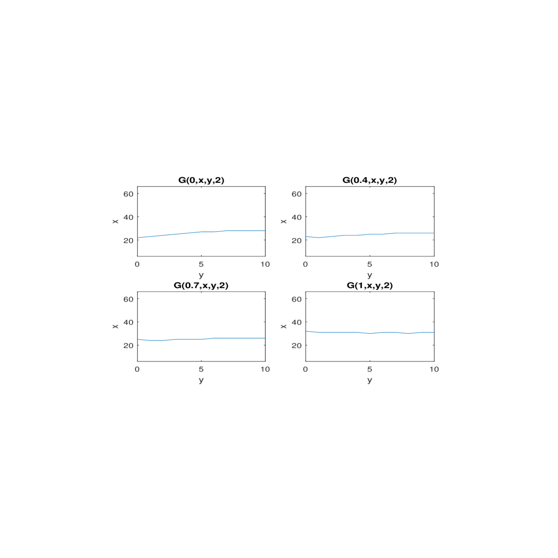
Figure 2: Plots of $G(s,x,y,i)$ at various times $s\in\{0,0.4,0.7,1\}$ when the market is down.

Appendix A Appendix: Proofs of Results

A.1 Proof of Lemma 3.2

In fact it can be shown that the value function are Lipschitz continuous with respect to $x$ and $y$. A detailed proof can be found in Pemy (2014) in the particular case of an optimal stopping problem. Below we show the linear growth property of the value function. The linear growth inequality follows from the Lipschitz continuity of the value function with respect to $x$ and $y$. Thus there exist $C,C^{\prime}>0$ such that

$$\begin{array}[]{rl}\displaystyle|V(s,x,y,i)|\leq C^{\prime}|x|+|V(s,0,y,i)|,\end{array}$$

and

$$\begin{array}[]{rl}\displaystyle|V(s,0,y,i)|\leq C|y|+|V(s,0,0,i)|.\end{array}$$

Combining the last two inequalities gives,

$$\begin{array}[]{rl}\displaystyle|V(s,x,y,i)|\leq\max(C^{\prime},C)(|x|+|y|+|V(s,0,0,i)|)\leq C_{0}(|x|+|y|+1),\end{array}$$

for some $C_{0}>\max(C^{\prime},C)$. This completes the proof.   $\sqcup\hbox to0.0pt{\hss$\sqcap$}$

A.2 Proof of Theorem 3.4

Let $\iota\in{\cal M}$, and $\psi\in\mathnormal{C}^{1,2,1}([0,T]\times{\mathbb{R}}^{+}\times[0,K])$ such that $V(s,x,y,\iota)-\psi(s,x,y)$ has local minimum at $(s_{0},x_{0},y_{0})$ in a neighborhood $N(s_{0},x_{0},y_{0})$. Without loss of generality we assume that $V(s_{0},x_{0},y_{0},\alpha_{0})-\psi(s_{0},x_{0},y_{0}).$ We set $\alpha(s_{0})=\alpha_{0}$ and define a function

$$\varphi(s,x,y,\iota)=\left\{\begin{array}[]{ll}\psi(s,x,y)&\textrm{if}\qquad i=\alpha_{0},\\ V(s,x,y,\iota),&\textrm{if}\qquad i\not=\alpha_{0}.\end{array}\right.$$ (27)

Let $\gamma\geq s_{0}$ be the first jump time of $\alpha(\cdot)$ from the initial state $\alpha(s_{0})=\alpha_{0}$, and let $\eta\in[s_{0},\gamma]$ be such that $(t,X(t),Y(t))$ starts at $(s_{0},x_{0},y_{0})$ and stays in $N(s_{0},x_{0},y_{0})$ for $s_{0}\leq t\leq\eta$. Moreover, $\alpha(t)=\alpha_{0}$, for $s_{0}\leq t\leq\eta$. Let $u(\cdot)$ be an admissible control such that $u(t)=u$ for $t\in[0,\eta]$. From then Dynamical Programming Principle (3.3) we derive

$$V(s_{0},x_{0},y_{0},\alpha_{0})\geq E\bigg{[}\int_{s_{0}}^{\eta}e^{-r(t-s_{0})}L(t,X(t),Y(t),u(t),\alpha(t))dt$$

$$+e^{-r(\eta-s_{0})}V(\eta,X(\eta),Y(\eta),\alpha(\eta))\bigg{]}.$$ (28)

Using Dynkin’s formula we have,

$$E^{s_{0},x_{0},y_{0},\alpha_{0}}[e^{-r(\eta-s_{0})}\varphi(\eta,X(\eta),Y(\eta),\alpha_{0})]-\varphi(s_{0},x_{0},y_{0},\alpha_{0})$$

$$= E^{s_{0},x_{0},y_{0},\alpha_{0}}\int_{s_{0}}^{\eta}e^{-r(t-s_{0})}[-r\varphi(t,X(t),Y(t),\alpha_{0})+({\cal L}^{u}\varphi)(t,X(t),Y(t),\alpha_{0})]dt.$$

where ${\cal L}^{u}$ is the generator of the Markov processes $(X_{t},Y_{t})$. Note that ${\cal L}^{u}(\varphi)(s,x,y,\iota)$ can be written as ${\cal L}^{u}(\varphi)(s,x,y,\iota)={\cal A}^{\iota,u}(\psi)(s,x,y)+Q\varphi(s,x,y,\cdot)(\iota)$ with

$$\begin{array}[]{rl}{\cal A}^{\iota,u}(\psi)(s,x,y)&\displaystyle=\frac{\partial\psi}{\partial s}+\frac{1}{2}\sigma^{2}(\iota)\frac{\partial^{2}\psi}{\partial x^{2}}+\kappa(\mu(i)-x)\frac{\partial\psi}{\partial x}-u\frac{\partial\psi}{\partial y}+\int_{{\mathbb{R}}}\bigg{(}\psi(s,x+\gamma(\iota)xz,y)\\ &\displaystyle-\psi(s,x,y)-{\bf 1}_{\{|z|<1\}}(z)\frac{\partial\psi(s,x,y)}{\partial x}\cdot\gamma(\iota)xz\bigg{)}\nu(dz).\end{array}$$

Given that $(s_{0},x_{0},y_{0})$ is the minimum of $V(t,x,y,\alpha_{0})-\psi(t,x,y)$ in $N(s_{0},x_{0},y_{0})$. For $s_{0}\leq t\leq\eta$, we have

$$V(t,X(t),Y(t),\alpha_{0})\geq\psi(t,X(t),Y(t))+V(s_{0},x_{0},y_{0},\alpha_{0})$$

$$-\psi(s_{0},x_{0},y_{0})=\varphi(t,X(t),Y(t),\alpha_{0}).$$ (30)

Using equation (27) and (A.2), we have

$$E^{s_{0},x_{0},y_{0},\alpha_{0}}[e^{-r(\eta-s_{0})}V(\eta,X(\eta),Y(\eta),\alpha_{0})]-V(s_{0},x_{0},y_{0},\alpha_{0})$$ (31)

$$\geq E^{s_{0},x_{0},y_{0},\alpha_{0}}\int_{s_{0}}^{\eta}e^{-r(t-s_{0})}\bigg{[}{\cal A}^{\alpha_{s_{0}},u}(\psi)(t,X(t),Y(t))+Q\varphi(t,X(t),Y(t),\cdot)(\alpha_{0})$$

$$-rV(t,X(t),Y(t),\alpha_{0})\bigg{]}dt.$$

Moreover, we have

$$Q\varphi(t,X(t),Y(t),\cdot)(\alpha_{0}) = \sum_{\beta\not=\alpha_{0}}q_{\alpha_{0}\beta}\Bigg{(}\varphi(t,X(t),Y(t),\beta)-\varphi(t,X(t),Y(t),\alpha_{0})\bigg{)}$$ (32)

$$\geq \sum_{\beta\not=\alpha_{0}}q_{\alpha_{0}\beta}\Bigg{(}V_{1}(t,X(t),Y(t),\beta)-V(t,X(t),Y(t),\alpha_{0})\bigg{)}$$

$$\geq QV_{1}(t,X(t),Y(t),\cdot)(\alpha_{0}).$$

It follows from (A.2), (31) and (32) that

$$\begin{array}[]{rl}\displaystyle E^{s_{0},x_{0},y_{0},\alpha_{0}}\int_{s_{0}}^{\eta}e^{-r(t-s_{0})}\bigg{[}{\cal A}^{\alpha_{0},u,}(\psi)(t,X(t),Y(t))+QV(t,X(t),Y(t),\cdot)(\alpha_{0})\\ -rV(t,X(t),Y(t),\alpha_{0})+L(t,X(t),Y(t),u(t),\alpha(t))\bigg{]}dt\leq 0.\end{array}$$

Dividing by $\eta-s_{0}>0$ and then sending $\eta\rightarrow s_{0}$ leads to

$$-rV(s_{0},x_{0},y_{0},\alpha_{0})+{\cal A}^{\alpha_{0},u}(\psi)(s_{0},x_{0},y_{0})$$

$$+QV(s_{0},x_{0},y_{0},\cdot)(\alpha_{0})+L(s_{0},x_{0},y_{0},u,\alpha_{0})\leq 0.$$ (33)

Since this inequality is true for any arbitrary control $u(t)\equiv u\in[0,\bar{u}]$, then taking the supremum over all values $u\in U=[0,\bar{u}]$ we have

$$\displaystyle rV(s_{0},x_{0},y_{0},\alpha_{0})-\sup_{u\in U}\Bigg{(}{\cal A}^{\alpha_{0},u}(\psi)(s_{0},x_{0},y_{0})$$

$$+QV(s_{0},x_{0},y_{0},\cdot)(\alpha_{0})+L(s_{0},x_{0},y_{0},u,\alpha_{0})\Bigg{)}\geq 0.$$ (34)

The inequalities (A.2) obviously proves that the value function $V$ is a viscosity supersolution as defined in (14).
Now, let us prove the subsolution inequality (13). We want to show that for each $\iota\in{\cal M}$,

$$rV(s_{0},x_{0},y_{0},\iota)-\sup_{u\in{U}}\Bigg{(}{\cal A}^{\alpha_{0},u}(\psi)(s_{0},x_{0},y_{0})$$

$$+QV(s_{0},x_{0},y_{0},\cdot)(\iota)+L(s_{0},x_{0},y_{0},u,\iota)\Bigg{)}\leq 0,$$ (35)

where $(s_{0},x_{0},y_{0})$ is a local maximum of $V(s,x,y,\iota)-\psi(s,x,y)$. Let us assume otherwise that the inequality (A.2) does not hold. In other terms, we assume that we can find a state $\alpha_{0}\in{\cal M}$, values $(s_{0},x_{0},y_{0})$ and a function $\phi\in{\cal C}^{1,2,1}([0,T]\times{\mathbb{R}}^{+}\times[0,K])$ such that $V(t,x,y,\alpha_{0})-\phi(t,x,y)$ has a local maximum at $(s_{0},x_{0},y_{0})\in[s,T]\times{\mathbb{R}}\times{\mathbb{R}}^{+},$ and we have

$$rV(s_{0},x_{0},y_{0},\alpha_{0})-\sup_{u\in{U}_{1}}\Bigg{(}{\cal A}^{\alpha_{0},u}(\psi)(s_{0},x_{0},y_{0})$$

$$+QV(s_{0},x_{0},y_{0},\cdot)(\alpha_{0})+L(s_{0},x_{0},y_{0},u,\alpha_{0})\Bigg{)}\geq\delta.$$ (36)

for some constant $\delta>0$.
Let us assume without loss of generality that $V(s_{0},x_{0},y_{0},\alpha_{0})-\phi(s_{0},x_{0},y_{0})=0$. We define

$$\varphi(s,x,y,i)=\left\{\begin{array}[]{ll}\phi(s,x,y),&\textrm{if}\qquad i=\alpha_{0},\\ V(s,x,y,i),&\textrm{if}\qquad i\not=\alpha_{0}.\end{array}\right.$$ (39)

Let $\gamma$ be the first jump time of $\alpha(\cdot)$ from the state $\alpha_{0}$, and let $\eta_{0}\in[s_{0},\gamma]$ be such that $(t,X(t),Y(t))$ starts at $(s_{0},x_{0},y_{0})$ and stays in $N(s_{0},x_{0},y_{0})$ for $s_{0}\leq t\leq\eta_{0}$. Since $\theta_{0}\leq\gamma$ we have $\alpha(t)=\alpha_{0}$, for $s_{0}\leq t\leq\eta_{0}$. Moreover, since $V(s_{0},x_{0},y_{0},\alpha_{0})-\phi(s_{0},x_{0},y_{0})=0$ and attains its maximum at $(s_{0},x_{0},y_{0})$ in $N(s_{0},x_{0},y_{0})$ then

$$V(\eta,X(\eta),Y(\eta),\alpha(\eta))\leq\phi(\eta,X(\eta),Y(\eta))\quad\hbox{for }\,\,\,s_{0}\leq\eta\leq\eta_{0}.$$

Thus, we also have

$$V(\eta,X(\eta),Y(\eta),\alpha(\eta))\leq\varphi(\eta,X(\eta),Y(\eta),\alpha(\eta))\quad\hbox{for }\,\,\,s_{0}\leq\eta\leq\eta_{0}.$$ (40)

Using the Dynamical Programming Principle (3.3), it clear that for any admissible control $u(\cdot)$ and time $\tau$ such that $s_{0}<\tau\leq\eta_{0}$, we have

$$\begin{array}[]{rl}\displaystyle J_{1}(s_{0},x_{0},y_{0},\alpha_{0};u)&\leq\displaystyle E^{s_{0},x_{0},y_{0},\alpha_{0}}\bigg{[}\int_{s_{0}}^{\tau}e^{-r(t-s_{0})}L(t,X(t),Y(t),u(t),\alpha(t))dt\\ &+e^{-r(\tau-s_{0})}V_{1}(\tau,X(\tau),Y(\tau),\alpha(\tau))\bigg{]}\\ &\displaystyle\leq E^{s_{0},x_{0},y_{0},\alpha_{0}}\bigg{[}\int_{s_{0}}^{\tau}e^{-r(t-s_{0})}L_{1}(t,X(t),u(t),,\alpha(t))dt\\ &+e^{-r(\tau-s_{0})}\varphi(\tau,X(\tau),Y(\tau),\alpha(\tau))\bigg{]}.\end{array}$$

Note that

$$Q\varphi(t,X(t),Y(t),\cdot)(\alpha_{0}) = \sum_{\beta\not=\alpha_{0}}q_{\alpha_{0}\beta}(V_{1}(t,X(t),Y(t),\beta)-\phi(t,X(t),Y(t)))$$ (41)

$$\leq \sum_{\beta\not=\alpha_{0}}q_{\alpha_{0}\beta}(V_{1}(t,X(t),Y(t),\beta)-V_{1}(t,X(t),Y(t),\alpha_{0}))$$

$$\leq QV_{1}(t,X(t),Y(t),\cdot)(\alpha_{0}).$$

Using the inequality (A.2) we have

$$J(s_{0},x_{0},y_{0},\alpha_{0};u)$$ (42)

$$\leq \displaystyle E^{s_{0},x_{0},y_{0},\alpha_{0}}\bigg{(}\int_{s_{0}}^{\tau}e^{-r(t-s_{0})}\bigg{\{}-\delta+rV(t,X(t),Y(t),\alpha_{0})$$

$$-{\cal A}^{\alpha_{0},u}(\phi)(t,X(t),Y(t))-QV(t,X(t),Y(t),\cdot)(\alpha_{0})\bigg{\}}dt\displaystyle$$

$$+e^{-r(\tau-s_{0})}\varphi(\tau,X(\tau),Y(\tau),\alpha_{0})\bigg{)}.$$

The Dynkin’s formula, (39) and (41) imply that

$$E^{s_{0},x_{0},y_{0},\alpha_{0}}e^{-r(\tau-s_{0})}\varphi(\tau,X(\tau),Y(\tau),\alpha_{0})$$ (43)

$$= E^{s_{0},x_{0},y_{0},\alpha_{0}}\int_{s_{0}}^{\tau}e^{-r(t-s_{0})}\Bigg{[}{\cal A}^{\alpha_{0},u,=}(\phi)(t,X(t),Y(t))+Q\varphi(t,X(t),Y(t),\cdot)(\alpha_{0})$$

$$-r\varphi(t,X(t),Y(t),\alpha_{0})\bigg{]}dt+\varphi(s_{0},x_{0},y_{0},\alpha_{0})$$

$$\leq E^{s_{0},x_{0},y_{0},\alpha_{0}}\int_{s_{0}}^{\tau}e^{-r(t-s_{0})}\Bigg{[}{\cal A}^{\alpha_{0},u}(\phi)(t,X(t),Y(t))+QV(t,X(t),Y(t),\cdot)(\alpha_{0})$$

$$-rV(t,X(t),Y(t),\alpha_{0})\bigg{]}dt+V(s_{0},x_{0},y_{0},\alpha_{0}).$$

Combining (42) and (43) we have

$$J(s_{0},x_{0},y_{0},\alpha_{0};u)\leq E^{s_{0},x_{0},y_{0},\alpha_{0}}\bigg{(}-\int_{s_{0}}^{\tau}e^{-r(t-s_{0})}\delta dt\bigg{)}+V(s_{0},x_{0},y_{0},\alpha_{0}).$$ (44)

It is easy to see that the quantity $\gamma=\displaystyle E^{s_{0},x_{0},y_{0},\alpha_{0}}\bigg{(}\int_{s_{0}}^{\tau}e^{-r(t-s_{0})}\delta dt\bigg{)}>0$, thus taking the supremum over all admissible control $u(\cdot)\equiv u$ we obtain

$$V(s_{0},x_{0},y_{0},\alpha_{0})\leq-\gamma+V(s_{0},x_{0},y_{0},\alpha_{0}),$$ (45)

which is a contradiction. This proves that the inequality (A.2) is satisfied. Obviously we derive the subsolution inequality (13). Therefore, $V$ is a viscosity solution of (11). The uniqueness of the viscosity solution follows from the standard Ishii method, for more one can refer to Pemy (2014) for a similar proof of the uniqueness of viscosity solution of optimal stopping problems for regime switching Lévy processes.   $\sqcup\hbox to0.0pt{\hss$\sqcap$}$

A.3 Proof of Lemma 4.1

We define the operator ${\cal F}_{\xi}$ on bounded functions on ${\cal D}_{R}$ as follows

$${\cal F}_{\xi}(V)(s,x,y,i;h,k,l)$$

$$= \frac{1}{r}\Delta_{s}V+\frac{1}{r}H_{u^{*},}^{j,k,l}V(s,x,y,i)$$

$$= \frac{1}{rk}V(s+k,x,y,i)+\sup_{u\in U}\Bigg{(}a(x,i)V(s,x+h,y,i)$$

$$+b(x,i)V(s,x-h,y,i)-c(x,i;u)V(s,x,y,i)-\frac{u}{rl}V(s,x,y+l,i)$$

$$+\sum_{j=0}^{N_{\xi}}\frac{c_{j}}{r}V(s,x+\gamma(i)z_{j}x,y,i)+\frac{1}{r}L(s,x,y,u,i)+\sum_{j\neq i}\frac{q_{ij}}{r}V(s,x,y,j)$$

$$-V(s,x+h,y,i)\frac{\sum_{j=0}^{M_{\xi}}d_{j}\gamma(i)z_{j}x}{rh}\Bigg{)}\quad\hbox{if }(s,x,y,i)\in{\cal D}_{R}\hbox{ and }s<T,$$

$${\cal F}_{\xi}(V)(T,x,y,i;h,k,l)=\Psi(T,x,y).$$

Where the coefficients $a(x,i),b(x,i)$ and $c(x,i;u)$ are defined as follows

$$\!\!\!\displaystyle c(x,i;u)=\frac{1}{rk}+\frac{\sigma^{2}(i)}{rh^{2}}+\frac{\kappa(\mu(i)-x)}{rh}-\frac{\sum_{j=0}^{M_{\xi}}d_{j}\gamma(i)xz_{j}}{rh}-\frac{u}{rl}+\frac{\Gamma}{r}+\sum_{j\neq i}\frac{q_{ij}}{r}$$ (47)

$$\!\!\!\displaystyle a(x,i)=\frac{\sigma^{2}(i)}{2rh^{2}}+\frac{\kappa(\mu(i)-x)}{rh},$$ (48)

$$\!\!\!\displaystyle b(x,i)=\frac{\sigma^{2}(i)}{2rh^{2}}.$$ (49)

Note that equation (21) is equivalent to $V(s,x,y,i)={\cal F}_{\xi}(V)(s,x,y,i;h,k,l)$, it suffices to show the operator ${\cal F}_{\xi}$ has a fixed point. Using the fact that the difference of sups is less than the sup of differences. If we have two bounded functions $V,W$ defined on ${\cal D}_{R}$, it is clear that

$$\begin{array}[]{rl}&\!\!\!\displaystyle|{\cal F}_{\xi}(V)(s,x,y,i;h,k,l)-{\cal F}_{\xi}(W)(s,x,y,i;h,k,l)|\\ &\!\!\!\displaystyle\leq\bigg{|}\sup_{u\in U}\bigg{[}\bigg{(}a(x,i;u)+b(s,x,i;u)-c(s,x,y,i;u)+\frac{1}{rk}+\sum_{j=0}^{N_{\xi}}\frac{c_{j}}{r}+\sum_{j\neq i}\frac{q_{ij}}{r}(u)\\ &\!\!\!\displaystyle-\frac{u}{rl}-\frac{\sum_{j=0}^{M_{\xi}}d_{j}\gamma(i)xz_{j}}{rh}\bigg{)}\sup_{{\cal D}_{R}}|V-W|\bigg{]}\bigg{|}\\ &\!\!\!\displaystyle\leq\bigg{|}\sum_{j=0}^{N_{\xi}}\frac{c_{j}}{r}-\frac{\Gamma}{r}\bigg{|}\sup_{{\cal D}_{R}}|V-W|.\end{array}$$

Therefore, for $\xi\in(0,1)$ small enough so that $\displaystyle\bigg{|}\sum_{j=0}^{N_{\xi}}\frac{c_{j}}{r}-\frac{\Gamma}{r}\bigg{|}<1$, the map ${\cal F}_{\xi}$ is a contraction on the space of bounded functions on ${\cal D}_{R}$, using the Banach’s Fixed Point Theorem we conclude the proof of the lemma.   $\sqcup\hbox to0.0pt{\hss$\sqcap$}$

A.4 Proof of Theorem 4.3

Define

$$\begin{array}[]{ll}V^{*}(s,x,y,i)&\!\!\!\displaystyle=\limsup_{\theta\to s,\eta\to x,\zeta\to y,k\downarrow 0,h\downarrow 0,l\downarrow 0}V_{k,h,l}(\theta,\eta,\zeta,i)\,\,\hbox{and}\\ V_{*}(s,x,y,i)&\!\!\!\displaystyle=\liminf_{\theta\to s,\eta\to x,\zeta\to y,k\downarrow 0,h\downarrow 0,l\downarrow 0}V_{k,h,l}(\theta,\xi,\zeta,i)\,\,.\end{array}$$ (52)

We claim that $V^{*}$ and $V_{*}$ are sub- and supersolutions of (11), respectively.

To prove this claim, we only consider the case for $V^{*}$. The argument for that of $V_{*}$ is similar. For each $i\in{\cal M}$, we want to show

$$\frac{\partial\Phi}{\partial s}(s_{0},x_{0},y_{0})\leq H(s_{0},x_{0},y_{0},i,V^{*},\frac{\partial\Phi}{\partial x},\frac{\partial\Phi}{\partial y},\frac{\partial^{2}\Phi}{\partial x^{2}}),$$

for any test function $\Phi\in{\cal C}^{1,2,1}([0,T]\times{\mathbb{R}}^{+}\times[0,K])$ such that $(s_{0},x_{0},y_{0},i)$ is a strictly local maximum of $V^{*}(s,x,y,i)-\Phi(s,x,y)$. Without loss of generality, we may assume that $V^{*}(s_{0},x_{0},y_{0},i)=\Phi(s_{0},x_{0},y_{0})$ and because of the stability of our scheme we can also assume that $\Phi\geq\sup_{k,h,l}\|V_{k,h,l}\|$ outside of the ball $B((s_{0},x_{0},y_{0}),r)$ where $r>0$ is such that

$$V^{*}(s,x,y,i)-\Phi(s,x,y)\leq 0=V^{*}(s_{0},x_{0},y_{0},i)-\Phi(s_{0},x_{0},y_{0})\ \hbox{ in }\ B((s_{0},x_{0},y_{0}),r).$$

This implies that there exist sequences $k_{n}>0$, $h_{n}>0$, $l_{n}>0$ and $(\theta_{n},\eta_{n},\zeta_{n})\in[0,T]\times{\mathbb{R}}^{+}\times[0,K]$ such that as $n\rightarrow\infty$ we have

$$\begin{array}[]{ll}&\!\!\!\displaystyle k_{n}\rightarrow 0,\,\,\,h_{n}\rightarrow 0,\,\,\,l_{n}\to 0,\,\,\,\theta\to s_{0},\,\,\,\eta_{n}\rightarrow x_{0},\,\,\,\zeta_{n}\rightarrow y_{0},\,\,\,V_{k_{n},h_{n},l_{n}}(\theta_{n},\eta_{n},\zeta_{n},i)\rightarrow V^{*}(s_{0},x_{0},y_{0},i),\\ &\!\!\!\displaystyle\hbox{and}\,\,\,(\theta_{n},\eta_{n},\zeta_{n})\,\hbox{ is a global maximum of }V_{k_{n},h_{n},l_{n}}-\Phi.\end{array}$$

Denote $\epsilon_{n}=V_{k_{n},h_{n},l_{n}}(\theta_{n},\eta_{n},\zeta_{n},i)-\Phi(\theta_{n},\eta_{n},\zeta_{n})$. Obviously $\epsilon_{n}\rightarrow 0$ and

$$V_{k_{n},h_{n},l_{n}}(s,x,y,i)\leq\Phi(s,x,y)+\epsilon_{n}\ \hbox{ for all }\ (s,x,y)\in[0,T]\times{\mathbb{R}}^{+}\times[0,K].$$ (54)

We know that for all $\xi\in(0,1)$,

$$S(\xi,k_{n},h_{n},l_{n},\theta_{n},\eta_{n},\zeta_{n},i,V_{k_{n},h_{n},l_{n}}(\theta_{n},\eta_{n},\zeta_{n},i),V_{k_{n},h_{n},l_{n}})=0.$$

The monotonicity of $S$ and (54) implies

$$\begin{array}[]{ll}&\!\!\!\displaystyle S(\xi,k_{n},h_{n},l_{n},\theta_{n},\eta_{n},\zeta_{n},i,\Phi(\theta_{n},\eta_{n},\zeta_{n})+\epsilon_{n},\Phi+\epsilon_{n})\\ &\displaystyle\ \leq S(\xi,k_{n},h_{n},l_{n},\theta_{n},\eta_{n},\zeta_{n},i,V_{k_{n},h_{n},l_{n}}(\theta_{n},\eta_{n},\zeta_{n},i),V_{k_{n},h_{n},l_{n}})=0.\end{array}$$ (57)

Therefore,

$$\lim_{\xi\downarrow 0}\lim_{n\to\infty}S(\xi,k_{n},h_{n},l_{n},\theta_{n},\eta_{n},\zeta_{n},i,\Phi(\theta_{n},\eta_{n},\zeta_{n})+\epsilon_{n},\Phi+\epsilon_{n})\leq 0,$$

so

$$\begin{array}[]{ll}&\!\!\!\displaystyle\frac{\partial\Phi}{\partial s}(s_{0},x_{0},y_{0})\leq H(s_{0},x_{0},y_{0},i,V^{*},\frac{\partial\Phi}{\partial x},\frac{\partial\Phi}{\partial y},\frac{\partial^{2}\Phi}{\partial x^{2}}).\end{array}$$

This proves that $V^{*}$ is a viscosity subsolution and, similarly we can prove that $V_{*}$ is a viscosity supersolution. Thus, using the uniqueness of the viscosity solution, we see that $V=V^{*}=V_{*}$. Therefore, we conclude that the sequence $(V_{h,k,l})_{h,k,l}$ converges locally uniformly to $V$ as desired.   $\sqcup\hbox to0.0pt{\hss$\sqcap$}$

References

- [1] N. Aleksandrov, R. Espinoza, and L. Gyurko, Optimal Oil Production and the World Supply of Oil, IMF Working Paper, WP/12/294, (2012)
- [2] G. Barles and P.E. Souganidis, Convergence of approximation schemes for fully nonlinear second order equations, Asymptot. Anal. 4, (1991), 271-283
- [3] R.E Beals, M. Gillis, G. Jenkins, and U. Peterson, Investment Polices: Issues and Analyses, in: M. Gillis, and R. E. Beals, eds: Tax and Investment Policies for Hard Minerals (Ballinger, Cambridge, MA), (1980), pp. 261-276.
- [4] S. Bhattacharyya, Energy Taxation and Environmental Externalities: a Critical Analysis, The Journal of Energy and Development, 22, (1998), pp. 199-220.
- [5] J. Cherian, J. Patel, and I. Khripko, Optimal Extraction of Nonrenewable Resources when Prices are Uncertain and Cost Cumulate, NUS Business School Working Paper, (Singapore:NUS), (1998).
- [6] M.G. Crandall and P. L. Lions, Viscosity solutions of Hamilton-Jacobi equations, Trans. Amer. Soc. 277, (1983), 1-42.
- [7] M. G. Crandall, H. Ishii, and P.L. Lions, User’s guide to viscosity solutions of second order partial differential equations, Bull. Amer. Math. Soc., 27, (1992), 1-67.
- [8] R. Gibson and E. S. Schwartz, Stochastic convenience yield and pricing of oil contingent claims, Journal of Finance, 45, (1990), pp. 959-976.
- [9] W. H. Fleming and R. Rishel Deterministic and Stochastic Optimal Control, New York, Springer-Verlag, 1975.
- [10] W. H. Fleming and H. M. Soner, Controlled Markov Processes and Viscosity Solutions, 2nd Ed., Springer, 2006.
- [11] J. D. Hamilton, A new approach to the economics analysis of nonstationary time series, Econometrica, 57, (1989), pp. 357-384.
- [12] D. A. Hanson, Increasing extraction costs and resource prices: Some further results. The Bell Journal of Economics, 11, 1, (1980), pp. 335-342.
- [13] T. Heaps and J. F. Helliwell, The Taxation of Natural Resources, Handbook of Public Economics, vol. 1, Eds A.J. Auerbach and M. Feldstein, Elsevier Science Piblishers B.V., North-Holland., 1985.
- [14] H. Hotelling, The economics of exhaustible resources, Journal of Political Economy, 39, 2, (1931), pp. 137-175.
- [15] H. Ishii, Uniqueness of unbounded viscosity solutions of Hamilton-Jacobi equations, Indiana Univ. Math. J. 33, (1984), 721-748.
- [16] H. J. Kushner, Probability Methods for Approximations in Stochastic Control and for Elliptic Equations, Academic Press, New York, 1977.
- [17] H. J. Kushner, P. G. Dupuis, Numerical Methods for Stochastic Control Problems in Continuous Time, Springer, New York, 1992.
- [18] C. Y. C. Lin and G. Wagner, Steady-state growth in Hotelling model of resource extraction, Journal of Environmental Economics and Management, 57, (2007), pp. 68-83.
- [19] B. Ksendal and Agnès Sulem, Applied Stochastic Control of Jump Diffusions , Springer, 2004
- [20] M. Pemy, Optimal selling rule in a regime switching Lévy Market, International Journal of Mathematics and Mathematical Sciences, 2011,(2011).
- [21] M. Pemy, Optimal stopping of Markov switching Lévy processes, Stochastics: An International Journal of Probability and Stochastic Processes, 86, 2, (2014), pp. 341-369.
- [22] Moustapha Pemy and Qing Zhang, Optimal stock liquidation in regime switching model with finite time horizon, Journal of Mathematical Analysis and Application, 321, Issue 2, (2006), 537- 552.
- [23] R. S. Pindyck, The optimal exploration and production of nonrenewable resources, The Journal of Political Economy, 86, 5, (1978) pp. 841-861.
- [24] R. S. Pindyck, Uncertainty and exhaustible resource markets, The Journal of Political Economy, 88, 6, (1980), pp. 1203-1225.
- [25] R. M. Solow and F. Y. Wan, Extraction costs in the theory of exhaustible resources, The Bell Journal of Economics, 7, 2 (1976), pp. 359-370.
- [26] E. Schwartz, Stochastic Behavior of Commodity Prices: Implications for valuation and Hedging, Journal of Finance, 52, (1997), pp. 923-973.
- [27] E. Schwartz and J. E. Smith, Short-Term Variations and Long-Term Dynamics in Commodity Prices, Management Science, 46, 7, (2000), pp. 893-911.
- [28] J. L. Sweeney, Economics of depletable resources: Market forces and intertemporal bias. The Review of Economics Studies, 44, 1, (1977), pp. 124-141.