Quantumness of Correlations in Fermionic Systems

Abstract

We present a new approach for the quantification of quantumness of correlations in fermionic systems. We study the Multipartite Relative Entropy of Quantumness in such systems, and show how the symmetries in the states can be used to obtain analytical solutions. Numerical evidences about the uniqueness of such solutions are also presented. Supported by these results, we show that the minimization of the Multipartite Relative Entropy of Quantumness, over certain choices of its modes multipartitions, reduces to the notion of Quantumness of Indistinguishable Particles. By means of an activation protocol, we characterize the class of states without quantumness of correlations. As an example, we calculate the dynamics of quantumness of correlations for a purely dissipative system, whose stationary states exhibit interesting topological non-local correlations.

I Introduction

The understanding of quantum correlations in systems of indistinguishable particles, especially fermions, is paramount for the development of materials supporting the new technologies of Quantum Information and Quantum Computation Nielsen and Chuang (2010); Nayak et al. (2008). The subtle notion of entanglement of indistinguishable particles has been investigated by many authors back in the 2000’s, with introduction of diverse seminal ideas like entanglement of modes Zanardi (2002), and entanglement of particles Wiseman and Vaccaro (2003); Eckert et al. (2002). Such ideas have been applied as new tools in the investigation of many-body system properties Amico et al. (2008), including the characterization of quantum phase transitions Iemini et al. (2015a); Amico et al. (2008).

From a mathematical viewpoint, the difficulty of understanding entanglement of indistinguishable particles stems from the absence of a tensor product structure in the Fock space, whereas the concept of entanglement is based on the non-separability, with respect to the tensor product, of a global state of identifiable subsystems. Friis et al. Friis et al. (2013) and Balachandran et al. Balachandran et al. (2013) have suggested interesting mathematical approaches to circumvent this obstacle. Our own efforts in this problem started with the proposal of entanglement witnesses for systems of indistinguishable particles Iemini et al. (2013), followed by appropriate adaptations of entropy of entanglement and negativity Iemini and Vianna (2013). More recently, extending the concept of quantumness of correlations Henderson and Vedral (2001); Ollivier and Zurek (2001); Modi et al. (2010); Debarba et al. (2012) to the realm of indistinguishable particles, we introduced the concept of quantumness of correlations of indistinguishable particles Iemini et al. (2014), which allowed us to devise a measurement procedure (dubbed an activation protocol) Piani et al. (2011); Streltsov et al. (2011) that determines the class of states without quantumness of correlations. In this activation protocol the quantumness of correlations of the system manifests itself as the smallest amount of bipartite entanglement created between system and measurement ancilla, during the local measurement protocol.

In order to recover the tensor product structure and the separability of the subsystems, one may use the isomorphism of the Fock space to a Hilbert space of distinguishable modes. This approach Zanardi (2002); Wiseman and Vaccaro (2003); Benatti et al. (2010); Bañuls et al. (2007) allows one to employ all the tools commonly used in distinguishable quantum systems for the analysis of the correlation between the modes of the system. The two notions of correlation in such systems, namely modes or particle correlation, follows naturally depending on the particular situation under scrutiny. For example, the correlations in eigenstates of a many-body Hamiltonian could be more naturally described by particle entanglement, whereas certain quantum information protocols could prompt a description in terms of entanglement of modes.

As the composed space of modes has a tensor product structure, given the modes are distinguishable, and there exists an isomorphism connecting the Hilbert space of modes and the Fock space of particles, some questions naturally arise: What is the relation between a correlated system of distinguishable modes and the correlations of indistinguishable particles? Is it possible to characterize or quantify the quantum correlations of particles by means of their mode quantum correlations? Can we characterize the set of uncorrelated states of indistinguishable particles out of the description of distinguishable modes? In this work we present a new approach for the quantumness of correlations of indistinguishable particles described by the minimization of the modes representation of the particles system. We show that, in the single particle partitioning, both notions are equivalent.

This work is organized as follows. In Sec. II, we present the formalism of Fock space for fermions, and its isomorphism with the Hilbert space of modes. In Sec. III, we present the local measurement formalism and introduce a quantifier of quantumness of correlations based on the local disturbance. We also present one of the main results of this work, proving that for quantum states with a given arbitrary symmetry, optimal local projective measurements - which minimize the local disturbance - are symmetric. In Sec. IV, we discuss the connection between quantumness of correlations of modes and quantumness of correlations of particles for single particle modes. In Sec. V, we characterize the set of fermionic states without quantumness of correlations. This results is obtained from an activation protocol for a system of L modes. In Sec. VI, we illustrate our results studying the dynamics of quantumness of correlations of a purely dissipative system. In Sec. VII, we analyze, numerically, the quantumness of correlations of more general symmetric quantum states and their respective local projectors. Conclusions are presented in Sec. VIII.

II Formalism

The space of quantum states for systems of indistinguishable fermions (bosons) is given by the anti-symmetric (symmetric) Hilbert-Schmidt subspace. Along all the paper, for simplicity, we will focus our calculations on the fermionic case, despite all results could be easily translated to the bosonic case. Formally, the quantum states for a fermionic system with $L$ modes are in the the Fock space ($\mathcal{F}_{L}$), namely,

$$\mathcal{F}_{L}=\mathopen{}\mathclose{{}\left|vac}\right\rangle\mathopen{}\mathclose{{}\left\langle vac}\right|\oplus\mathcal{A}(\mathcal{H}^{L})\oplus\mathcal{A}(\mathcal{H}^{L}\otimes\mathcal{H}^{L})\oplus...\oplus\mathcal{A}(\mathcal{H}^{L^{\otimes L}}),$$

i.e., the direct sum of anti-symmetric Hilbert spaces ($\mathcal{A}(\mathcal{H}^{L^{\otimes N}})$) with fixed $N=0,1,...,L$ fermions, with $|vac\rangle$ being the vacuum state. Recall that the direct sum is defined as:

$$A\oplus B=\mathopen{}\mathclose{{}\left[\begin{array}[]{cc}A&0\\ 0&B\end{array}}\right].$$ (1)

The dimension of the Fock space is given by:

$$N_{F}^{L}=\sum_{i=0}^{L}\frac{L!}{(L-i)!i!}=2^{L}.$$ (2)

A basis can be generated from a set of single-particle fermionic operators $\{a_{j}\}_{j=1}^{L}$ for the $L$ modes, satisfying the canonical anti-commutation relations:

$$\{a_{i},a_{j}^{\dagger}\}=\delta_{ij},\,\,\,\{a_{i},a_{j}\}=0.$$ (3)

We represent the basis with the short notation,

$$|a^{\dagger}_{\vec{j}}\rangle\equiv(a^{\dagger}_{1})^{j_{1}}(a^{\dagger}_{2})^{j_{2}}...\,(a^{\dagger}_{L})^{j_{L}}\mathopen{}\mathclose{{}\left|vac}\right\rangle,$$ (4)

with $\vec{j}=(j_{1},...,j_{L})$, and $j_{i}=0(1)$ denoting an empty (occupied) mode.

By means of the occupation-number representation, the Fock space can be associated to a Hilbert space of $L$ qubits with a $2^{L}$-dimensional basis, $\{\mathopen{}\mathclose{{}\left|j_{1}j_{2}\ldots j_{L}}\right\rangle\}$, where $j_{\ell}$ is $0$ or $1$ for unoccupied or occupied modes, respectively.

Formally, these two equivalent representations are related by the following isomorphism $\Lambda$:

$$\Lambda:\mathcal{F}_{L} \longleftrightarrow \mathcal{H}^{2}_{1}\otimes\cdots\otimes\mathcal{H}^{2}_{L}$$ (5)

$$|a^{\dagger}_{\vec{j}}\rangle\equiv(a^{\dagger}_{1})^{j_{1}}...\,(a^{\dagger}_{L})^{j_{L}}\mathopen{}\mathclose{{}\left|vac}\right\rangle \longleftrightarrow \mathopen{}\mathclose{{}\left|j_{1}}\right\rangle\otimes...\otimes\mathopen{}\mathclose{{}\left|j_{L}}\right\rangle\equiv|\vec{j}\rangle,$$

which maps the Fock space into the space of $L$ distinguishable modes (qubits in the fermionic case). We will denote hereafter as “configuration representation (modes representation)” the left (right) side of the previous equation. Notice that, in principle, the basis $\{a_{j}\}_{j=1}^{L}$ of fermionic operators is arbitrarily chosen, and the previous isomorphism is completely dependent on it. Therefore different modes representations can be obtained by means of a unitary transformation on the Fock space $U\in\mathcal{U}(\mathcal{F}_{L})$, named Bogoliubov transformations,

$$\tilde{f}^{\dagger}_{k}=\sum_{j}U_{kj}a^{\dagger}_{j},$$ (6)

where $\{\tilde{f}^{\dagger}_{k}\}_{k=1}^{L}$ and $\{a^{\dagger}_{j}\}_{j=1}^{L}$ are single particle fermionic operators.

III Quantumness of Correlations

In this section we will first introduce the description of local measurements on the modes. In this context, we will introduce a quantifier of quantumness of correlations based on the smallest disturbance created by local measurements. We will then be ready to present one of our main results, proving that for quantum states with a given arbitrary symmetry, the optimal local projective measurement, i.e., the local projectors which creates the smallest disturbance in the state, is that which shares the same symmetry with the quantum state.

Let us first formally define the concept of projective measurement. Given a general bi-partition of the $L$ modes as $j_{A}$/$j_{B}$, with $j_{B}=L-j_{A}$, a general set of local projective measurements $\{\hat{\Pi}^{(j_{A})}_{m}\}_{m}$ acting on $j_{A}$ is defined as:

$$\hat{\Pi}_{m}^{(j_{A})}\hat{\Pi}_{n}^{(j_{A})} = \delta_{m,n}\hat{\Pi}_{m}^{(j_{A})},$$ (7)

$$\sum_{m}\hat{\Pi}_{m}^{(j_{A})} = \mathbb{I}.$$ (8)

The quantum state $\rho\in\mathcal{D}(\mathcal{H}^{2j_{A}}\otimes\mathcal{H}^{2j_{B}})$, where $\mathcal{D}$ denotes the set of all positive semi-definite operators, after such measurement is described as a local dephased state, given by:

$$\Pi^{(j_{A})}(\rho) = \sum_{m}\hat{\Pi}_{m}^{(j_{A})}\rho\hat{\Pi}_{m}^{(j_{A})}$$ (9)

$$= \sum_{m}\text{Tr}_{j_{A}}(\hat{\Pi}_{m}^{(j_{A})}\rho)\,\hat{\Pi}_{m}^{(j_{A})}$$

$$= \sum_{m}p_{\Pi_{m}}^{(j_{A})}\,\hat{\Pi}_{m}^{(j_{A})}\otimes\sigma_{m}^{(j_{B})},$$

where

$$p_{\Pi_{m}}^{(j_{A})}=\text{Tr}(\hat{\Pi}_{m}^{(j_{A})}\rho),\qquad\sigma_{m}^{(j_{B})}=\frac{1}{p_{\Pi_{m}}^{(j_{A})}}\text{Tr}_{j_{A}}(\hat{\Pi}_{m}^{(j_{A})}\rho),$$ (10)

with $\sigma_{m}^{(j_{B})}$ representing the reduced state, which might be a mixed state, in the complementary $j_{B}$ subspace.

The quantification of quantumness of correlations in a quantum system can be performed by means of the smallest disturbance created by a local measurement Brodutch and Modi (2012). Such disturbance could be quantified as the distance between the original state and the measured one Luo (2008); Debarba et al. (2012); Nakano et al. (2012); Modi et al. (2010). In this way we define the multipartite relative entropy of quantumness Modi et al. (2010); Oppenheim et al. (2002):

Definition 1 (Multipartite Relative Entropy of Quantumness- MREQ).

Given an arbitrary multipartite quantum state $\rho\in\mathcal{D}(\mathcal{H}_{1}\otimes\cdots\otimes\mathcal{H}_{n})$ and a set $\Sigma\subseteq\{1,2,\dots,n\}$, the Multipartite Relative Entropy of Quantumness on the subsystems $\Sigma$ is defined as :

$$Q^{\Sigma}(\rho)=\min_{\{\bigotimes_{j\in\Sigma}\Pi^{(j)}\}}S\mathopen{}\mathclose{{}\left(\rho\mathopen{}\mathclose{{}\left|}\right|\bigotimes_{j\in\Sigma}\Pi^{(j)}(\rho)}\right)$$ (11)

where $\Pi^{(j)}(\rho)$ is a local projective measurement map over the $j$’th partition of $\rho$ and $S(\rho||\sigma)=-S(\rho)-Tr(\rho\log\sigma)$ is the relative entropy between $\rho$ and $\sigma$, with $S(\rho)$ the von Neumann entropy.

Considering a bi-partition on the modes, $\rho\in\mathcal{D}(\mathcal{H}_{A}\otimes\mathcal{H}_{B})$, and restricting the set $\Sigma=A$, the relative entropy is the quantifier of quantumness of correlations corresponding to the One-Way Work Deficit Oppenheim et al. (2002):

$$Q^{(A)}(\rho) = \min_{\{\Pi^{A}\}}S(\rho||\Pi^{A}(\rho))$$ (12)

$$= \min_{\{\Pi^{A}\}}\mathopen{}\mathclose{{}\left[S(\Pi^{A}(\rho))-S(\rho)}\right].$$

The computation of the above quantifiers is not a trivial task, in general, due to the minimization over all local projective measurements. The solution of the above minimization might not even be unique; however, by definition, it is always a set of rank-1 local projectors Horodecki et al. (2005). One could try to use some information of the quantum state under analysis in order to solve the optimization, or at least to restrict the search of the optimal projective measurement to a subset. In the context of ensemble of quantum states generated by a symmetric group, it is known that the POVM which optimizes the accessible information is also created by the symmetric group Ban et al. (1997). It is analogous to the quantum state discrimination problem, where the concerned states and the optimal POVM have the same symmetry Sasaki et al. (1999); Davies (1978). In Ref.Chiribella and Mauro D’Ariano (2006), it is shown that, under the action of a symmetric group in the probability space, the extremal covariant POVMs are in one-to-one correspondence to the convex set of block diagonal operators on the Hilbert space. Therefore symmetries can be written as degenerated observables. Following this approach, we will show here that, in the context of quantumness of correlations, if the quantum state has a given symmetry, the minimization task can be performed restricted to symmetric projective measurements. This simplification follows from the following Lemma.

Lemma 1.

Consider a symmetry $\hat{\Theta}\in\mathcal{L}(\mathcal{H}_{1}\oplus\cdots\oplus\mathcal{H}_{N})$, where $\mathcal{L}(\cdots)$ denotes the set of linear operators, $\theta_{j}$ are the eigenvalues of the symmetry and $\mathcal{H}_{j}$ their corresponding block diagonal subspace. Given a quantum state $\rho\in\mathcal{D}(\mathcal{{H}}_{j}=\mathcal{{H}}_{j}^{A}\otimes\mathcal{{H}}_{j}^{B})$, i.e., a quantum state with non trivial projection onto a single eigenvalue of the symmetry, there exists a set of symmetric local projective measurements $\{\hat{P}_{\ell}^{(A)}\}_{\ell}$ that is a solution of the One-Way Work Deficit - Eq.(12). This projective measurement acts locally on the $A$ bi-partition, either preserving the state symmetry, $\hat{P}_{\ell}^{(A)}\rho\hat{P}_{\ell}^{(A)}\in\mathcal{D}(\mathcal{{H}}_{j})$, or annihilating the state, $\hat{P}_{\ell}^{(A)}\rho\hat{P}_{\ell}^{(A)}=0$, in case the symmetry subspace defined by $\hat{P}_{\ell}^{(A)}$ is orthogonal to the state symmetry.

According to the Lemma, the set of symmetric projective measurements creates the smallest disturbance in the symmetric state. It explores the block diagonal structure of the symmetry, in the sense that an optimal symmetric projective measurement must preserve such structure. Consequently we have a great simplification of the optimization problem in the computation of the relative entropy of quantumness. As we will discuss in the next section, for some symmetries and modes partitions, there exists a unique projective measurement satisfying the Lemma conditions, thus allowing us to compute the quantumness analytically. The proof for the Lemma 1 is given in the Appendix.

Example. Let us present a simple example illustrating the previous discussion. Assume a bipartite distinguishable system ($A-B$) in a state with the following Schmidt decomposition:

$$\mathopen{}\mathclose{{}\left|\psi}\right\rangle=\sum_{i=1}^{r}\sqrt{p_{i}}\mathopen{}\mathclose{{}\left|a_{i}}\right\rangle\mathopen{}\mathclose{{}\left|b_{i}}\right\rangle.$$ (13)

If $\{\mathopen{}\mathclose{{}\left|a_{i}}\right\rangle\}$ is an orthonormal basis in the Hilbert space of a qubit, while $\{\mathopen{}\mathclose{{}\left|b_{i}}\right\rangle\}$ is an orthonormal basis for a Hilbert space of arbitrary finite dimension, then $r$ is at most 2. Consider a local projective measurement in the Schmidt basis,

$$\Pi^{A}_{1}=\mathopen{}\mathclose{{}\left|a_{1}\middle\rangle\middle\langle a_{1}}\right|\otimes\mathbb{I}_{B},\quad\hat{\Pi}^{A}_{2}=\mathopen{}\mathclose{{}\left|a_{2}\middle\rangle\middle\langle a_{2}}\right|\otimes\mathbb{I}_{B}.$$ (14)

Then we have:

$$\Pi^{A}(\rho) = \hat{\Pi}^{A}_{1}\rho\hat{\Pi}^{A}_{1}+\hat{\Pi}^{A}_{2}\rho\hat{\Pi}^{A}_{2}\$$ (15)

$$= p_{1}\mathopen{}\mathclose{{}\left|a_{1}b_{1}\middle\rangle\middle\langle a_{1}b_{1}}\right|+(1-p_{1})\mathopen{}\mathclose{{}\left|a_{2}b_{2}\middle\rangle\middle\langle a_{2}b_{2}}\right|$$

with

$$\mathopen{}\mathclose{{}\left\langle\psi}\right|(\mathopen{}\mathclose{{}\left|a_{1}\middle\rangle\middle\langle a_{1}}\right|\otimes\mathbb{I}_{B})\mathopen{}\mathclose{{}\left|\psi}\right\rangle = p_{1}$$ (16)

$$\mathopen{}\mathclose{{}\left\langle\psi}\right|(\mathopen{}\mathclose{{}\left|a_{2}\middle\rangle\middle\langle a_{2}}\right|\otimes\mathbb{I}_{B})\mathopen{}\mathclose{{}\left|\psi}\right\rangle = (1-p_{1})$$ (17)

and the relative entropy for such local measurement is given by,

$$S(\rho||\Pi^{A}(\rho))=h(p_{1})=-p_{1}\log{p_{1}}-(1-p_{1})\log(1-p_{1}).$$

Thus we have determined the entropy of entanglement of this system ($E(\rho)=S(\rho_{A})=h(p_{1})$, with $\rho_{A}=Tr_{B}(\rho)$) by means of local projective measurements. A lesson here is that it would be easy to measure entanglement if we knew the Schmidt basis. Let us check what bound we would obtain measuring in an arbitrary local basis, namely:

$$\mathopen{}\mathclose{{}\left|\tilde{a}_{i}}\right\rangle=\alpha_{1i}\mathopen{}\mathclose{{}\left|a_{1}}\right\rangle+\alpha_{2i}\mathopen{}\mathclose{{}\left|a_{2}}\right\rangle,$$ (18)

$$\mathopen{}\mathclose{{}\left\langle\tilde{a}_{i}\middle|\tilde{a}_{j}}\right\rangle=\delta_{ij},$$

that is,

$$\mathopen{}\mathclose{{}\left|\tilde{a}_{i}}\right\rangle=U\mathopen{}\mathclose{{}\left|a_{i}}\right\rangle,$$ (19)

where $U$ is an arbitrary unitary transformation. Now, if we perform a local projective measurement in the basis $\{\mathopen{}\mathclose{{}\left|\tilde{a}_{i}}\right\rangle\}$, we obtain:

$$\tilde{p}_{1}=\mathopen{}\mathclose{{}\left\langle\psi}\right|(\mathopen{}\mathclose{{}\left|\tilde{a}_{1}\middle\rangle\middle\langle\tilde{a}_{1}}\right|\otimes\mathbb{I}_{B})\mathopen{}\mathclose{{}\left|\psi}\right\rangle,$$ (20)

$$\tilde{p}_{1}=\mathopen{}\mathclose{{}\left|\alpha_{11}}\right|^{2}p_{1}+\mathopen{}\mathclose{{}\left|\alpha_{21}}\right|^{2}(1-p_{1}).$$

As the binary entropy is a concave function, we have:

$$h(\tilde{p}_{1})\geq\mathopen{}\mathclose{{}\left|\alpha_{11}}\right|^{2}h(p_{1})+\mathopen{}\mathclose{{}\left|\alpha_{21}}\right|^{2}h(1-p_{1}),$$ (21)

$$\Rightarrow h(\tilde{p}_{1})\geq h(p_{1}).$$

Therefore, a measurement in an arbitrary basis gives us an upper bound for the relative entropy, and we could obtain the quantumness of correlations - One-Way Work Deficit - by a minimization over all different bases:

$$Q^{A}(\psi)=\min_{U}h(\tilde{p}_{1}).$$ (22)

Now we will proceed to the case of a system of indistinguishable fermions, and discuss how some symmetries of the quantum state can be useful in determining the optimal local measurements for the relative entropy.

We shall discuss the case of states with definite parity. Consider the following projectors onto a single particle mode:

$$\hat{\Pi}_{j}=a_{j}^{\dagger}a_{j},\,\,\,\hat{\Pi}_{\bar{j}}=a_{j}a_{j}^{\dagger},\,\,\,\hat{\Pi}_{j}+\hat{\Pi}_{\bar{j}}=1.$$ (23)

Now an arbitrary Fock state with definite parity can be written as:

$$\mathopen{}\mathclose{{}\left|\psi}\right\rangle=\hat{\Pi}_{j}\mathopen{}\mathclose{{}\left|\psi}\right\rangle+\hat{\Pi}_{\bar{j}}\mathopen{}\mathclose{{}\left|\psi}\right\rangle=\sqrt{p_{j}}\mathopen{}\mathclose{{}\left|\psi_{j}}\right\rangle+\sqrt{p_{\bar{j}}}\mathopen{}\mathclose{{}\left|\psi_{\bar{j}}}\right\rangle,$$ (24)

where we have defined the following state:

$$\mathopen{}\mathclose{{}\left|\psi_{j}}\right\rangle=\frac{\hat{\Pi}_{j}\mathopen{}\mathclose{{}\left|\psi}\right\rangle}{\sqrt{p_{j}}},\quad p_{j}=\langle{\psi}|\hat{\Pi}_{j}|\psi\rangle,$$ (25)

and analogously for $\mathopen{}\mathclose{{}\left|\psi_{\bar{j}}}\right\rangle$. These projectors (Eq.23) define a bi-partition in the Fock space and directly determine the Schmidt decomposition for the state. $\mathopen{}\mathclose{{}\left|\psi_{j}}\right\rangle$ is in the subspace where the mode $j$ is occupied, whereas $\mathopen{}\mathclose{{}\left|\psi_{\bar{j}}}\right\rangle$ is in the complementary subspace.

Recalling the previous discussion for general states (Eq.(13)), we easily conclude that the local measurement from these projectors determine the quantumness of correlations - One-Way Work Deficit - for the state. Notice that the measurement preserves the symmetry of the state, according to the Lemma, and the above rationale is valid for arbitrary states with parity symmetry.

IV Equivalence between Quantumness of Correlations of Modes and Particles

In this section we will discuss the implication of Lemma 1 in the context of quantum states with fixed parity symmetry. In particular, we show that the notion of Quantumness between Indistinguishable Particles can be recovered from quantumness between modes, by analyzing the minimum of the Multipartite Relative Entropy of Quantumness over certain choices of modes multipartitions.

Since the quantumness of correlations is implicitly related to local measurements on composite systems, the characterization, or even a proper definition, of the quantumness of correlations between indistinguishable particles is a much subtler task. In such systems particles are no longer accessible individually, thus eliminating the usual notions of separability and local measurements. In Ref.Iemini et al. (2014), the authors define such a notion of quantumness of correlations between indistinguishable particles by means of the activation protocol, which relates the correlations to the smallest amount of entanglement created between system and apparatus during a single particle measurement. As system and apparatus are always distinguishable, the quantumness of correlations of a indistinguishable system can be obtained from usual distinguishable quantities.

Let us recall the measure of quantumness of correlations as proposed in Ref.Iemini et al. (2014):

Definition 2 (Quantumness of correlations between indistinguishable particles).

Considering a system of particles described by the density matrix $\rho\in\mathcal{D}({\mathcal{F}_{L}})$, the quantumness of correlations between the indistinguishable particles is defined by means of the relative entropy, as follows :

$$\mathcal{Q}_{p}^{\emptyset}(\rho)=\min_{V\in\mathcal{U}({\mathcal{F}_{L}})}S(\rho||\hat{\Pi}^{V}(\rho)),$$ (26)

where

$$\hat{\Pi}^{V}(\rho)=\sum_{\{\vec{\ell}\}}\langle a_{\vec{\ell}}|V^{\dagger}\rho V|a_{\vec{\ell}}\rangle\,|a_{\vec{\ell}}\rangle\langle a_{\vec{\ell}}|,$$ (27)

with $\{\mathopen{}\mathclose{{}\left|a_{\vec{\ell}}}\right\rangle\}$ being a single Slater determinant basis, as defined in Eq.(4), and $V$ a unitary transformation on Fock space, as defined in Eq.(6).

An important consequence of the Lemma follows for quantum states with fixed parity symmetry. Considering a bi-partition of the modes between a single-particle mode “$a_{j}$” with the rest of the system, the set of rank-$1$ local projective measurements onto such mode, preserving the symmetry of the state, reduces to a single possible set (and thus a solution for the One-Way Work Deficit):

$$\hat{\Pi}^{j}_{min}=\mathopen{}\mathclose{{}\left\{\hat{\Pi}^{j}_{0}=a_{j}a_{j}^{\dagger},\,\hat{\Pi}^{j}_{1}=a_{j}^{\dagger}a_{j}}\right\}.$$ (28)

In the case of a multi-partition of the system in $L$ subsystems, with each one corresponding to a single-particle mode $a_{j}$, the set of rank-$1$ local projective measurements onto such subsystems, preserving the symmetry of the state, reduces to:

$$\hat{\Pi}^{1\,2...L}_{min}=\mathopen{}\mathclose{{}\left\{\hat{\Pi}^{1}_{\ell}\otimes\hat{\Pi}^{2}_{\ell}\otimes\cdots\otimes\hat{\Pi}^{L}_{\ell}}\right\},\quad(\ell=0,1),$$ (29)

and thus represents the constrained set solution for the MREQ.

With the previous considerations, we are now ready to present one of the most important results of this work. We relate the notion of quantumness of correlations between indistinguishable particles to the MREQ minimized over all possible single-particle modes partitions.

Theorem 1.

Given a system with $L$ modes, described by the state $\rho\in\mathcal{D}(\mathcal{H}_{1}^{2}\otimes\cdots\otimes\mathcal{H}_{L}^{2})$ with fixed parity symmetry (cf Lemma), the minimization of the Multipartite Relative Entropy of Quantumness, over all single-particle representations “$\{a\}$”, is equal to the Quantumness of correlations between indistinguishable particles:

$$\mathcal{Q}^{\emptyset}_{p}(\rho)=\min_{\{a\}}Q_{a}^{1,\ldots,L}(\rho),$$ (30)

where $a:\mathcal{F}_{L}\leftrightarrow\mathcal{H}^{2\otimes L}$ represents the isomorphism between Fock and modes space (Eq.(5)), and ${1,\ldots,L}$ indicates that the measurement is performed locally over all modes.

Proof.

Given the relative entropy of quantumness for the modes, perform a measurement over all of them locally, in a representation $\Lambda$:

$$Q^{1,\ldots,L}_{a}(\rho)=\min_{\Pi^{a}}S(\rho\|\Pi^{a}(\rho))=S(\rho\|\Pi^{a}(\rho)),$$

where $\Pi^{a}(\rho)$ is the local measurement map over all modes in the representation $a$. By means of Lemma 1, the minimization over all projective measurements in this representation is restricted to only one projective measurement map $\Pi^{a}$. The projective measurement map acts on $\rho$ as:

$$\Pi^{a}(\rho) =\hat{\Pi}_{1}^{a}\otimes\cdots\otimes\hat{\Pi}_{L}^{a}(\rho)$$

$$=\sum_{\vec{l}}\hat{\Pi}_{\vec{l}}\rho\hat{\Pi}_{\vec{l}}$$

$$=\sum_{\vec{l}}\mathopen{}\mathclose{{}\left|a_{\vec{\ell}}\middle\rangle\middle\langle a_{\vec{\ell}}}\right|\rho\mathopen{}\mathclose{{}\left|a_{\vec{\ell}}\middle\rangle\middle\langle a_{\vec{\ell}}}\right|,$$

where $\mathopen{}\mathclose{{}\left|a_{\vec{\ell}}}\right\rangle=a_{\vec{l}}\mathopen{}\mathclose{{}\left|vac}\right\rangle=a_{1}^{l_{1}\dagger}\cdots a_{L}^{l_{L}\dagger}\mathopen{}\mathclose{{}\left|vac}\right\rangle$. The transformation from the representation $\Lambda$ to another $\Lambda^{\prime}$ can be performed by means of a Bogoliubov transformation $V$, thus:

$$f_{\vec{l}}^{\dagger}=Va_{\vec{l}}^{\dagger},$$

where ${V}$ is a unitary operation on the particles. Therefore minimizing the quantumness of modes over all representations amounts to minimize it over all Bogoliubov transformations $V$:

$$\min_{\Pi^{a}}S(\rho\|\Pi^{a}(\rho))=\min_{V}S(\rho\|\Pi^{V}(\rho)),$$

where

$$\Pi^{V}(\rho)=\sum_{l}\mathopen{}\mathclose{{}\left\langle a_{\vec{\ell}}}\right|V^{\dagger}\rho V\mathopen{}\mathclose{{}\left|a_{\vec{\ell}}}\right\rangle\mathopen{}\mathclose{{}\left|a_{\vec{\ell}}\middle\rangle\middle\langle a_{\vec{\ell}}}\right|,$$

which results in the measure of quantumness of correlations defined in Eq.26. ∎

Theorem 1 determines a new approach for the quantification of correlations between indistinguishable particles. Motivated by this result, it would be interesting to study the minimum of the single-mode correlations, described by the One-Way Work Deficit in Eq.(12), over all possible single-particle representations. Recently, Gigena and Rossignoli explored this idea in entangled pure states with parity symmetry Gigena and Rossignoli (2015), and also investigated the one-body information loss Gigena and Rossignoli (2016). By means of Lemma 1, one can see that these two notions are indeed the one-way work deficit for fermions, as we describe below. A direct implication of Lemma 1 is the analytical computation of the One-Way Work Deficit for a single-particle mode:

$$Q^{j}_{a}(\rho)=S\mathopen{}\mathclose{{}\left(a^{\dagger}_{j}a_{j}\rho a^{\dagger}_{j}a_{j}+a_{j}a^{\dagger}_{j}\rho a_{j}a^{\dagger}_{j}}\right)-S(\rho),$$ (31)

where now we write $Q^{j}_{a}\equiv Q^{(j)}$, in order to make clear that we deal with the quantumness of correlations of a single-particle mode $a_{j}$. In particular, if the quantum state is pure ($|\psi\rangle$), the One-Way Work Deficit is given by,

$$Q^{j}_{a}(\mathopen{}\mathclose{{}\left|\psi}\right\rangle)=H\mathopen{}\mathclose{{}\left(\langle a^{\dagger}_{j}a_{j}\rangle,\langle a_{j}a^{\dagger}_{j}\rangle}\right).$$ (32)

Summing the single-particle correlation of all modes, $\sum_{j=1}^{L}Q^{j}_{a}({\rho})$, gives us the correlation in this particular basis of modes, with minimum correlation in its single-particle modes, defining in this way the One-Body Quantumness of Correlations:

$$\mathcal{Q}_{sp}(\rho)=\min\limits_{\{a\}}\mathopen{}\mathclose{{}\left(\sum_{j=1}^{L}Q^{j}_{a}(\rho)}\right).$$ (33)

As the quantifier in Eq.(12), the One-Body Quantumness of Correlations is obtained by means of a quantifier of quantumness of correlations based on the tensor product construction of distinguishable systems. This is of paramount importance, for it circumvents any controversy about correlations in Fock space. As discussed above, for single-particle modes partitioning there exists only one projector that minimizes the local disturbance for symmetric states, then it is simple to show the equivalence of the quantumness of correlations defined via one-way work deficit in Eq.(12), and the entanglement measure proposed in Ref.Gigena and Rossignoli (2015) for pure states.

Theorem 2.

For a pure state $\mathopen{}\mathclose{{}\left|\psi}\right\rangle\in\mathcal{H}^{2}\otimes\mathcal{H}^{2(L-1)}$, the one-body quantumness of correlations and the one-body entanglement are given by:

$$S_{sp}(\mathopen{}\mathclose{{}\left|\psi}\right\rangle)=\mathcal{Q}_{sp}(\mathopen{}\mathclose{{}\left|\psi}\right\rangle)=\min\limits_{\{a\}}\mathopen{}\mathclose{{}\left(\sum_{j=1}^{L}Q^{j}_{a}(\mathopen{}\mathclose{{}\left|\psi}\right\rangle)}\right),$$ (34)

where $\mathcal{E}_{sp}$ is the entropy of entanglement for pure states of particles, as proposed in Ref.Gigena and Rossignoli (2015).

Proof.

Considering the optimal projective measurement described by the map $\Pi_{j}^{a}$ with projectors $\{a_{j}a_{j}^{\dagger},a_{j}^{\dagger}a_{j}\}$, the quantumness of correlations in this mode representation is:

$$\mathcal{{Q}}_{sp}^{a}(\mathopen{}\mathclose{{}\left|\psi}\right\rangle)\equiv\sum_{j}Q_{a}^{j}(\mathopen{}\mathclose{{}\left|\psi}\right\rangle)=\sum_{j}S(\Pi^{a}_{j}(\mathopen{}\mathclose{{}\left|\psi}\right\rangle)),$$

where $\Pi_{j}^{a}(\psi)=\langle a^{\dagger}_{j}a_{j}\rangle\mathopen{}\mathclose{{}\left|\phi_{o}\middle\rangle\middle\langle\phi_{o}}\right|+\langle a_{j}a^{\dagger}_{j}\rangle|{\phi_{e}}\rangle\langle{\phi_{e}}|$ is a projective measurement described in Eq.(28). As this measurement is composed by rank-1 projectors, the states $\mathopen{}\mathclose{{}\left|\phi_{o}}\right\rangle$ and $\mathopen{}\mathclose{{}\left|\phi_{e}}\right\rangle$ are orthogonal, therefore:

$$\mathcal{{Q}}_{sp}^{a}(\mathopen{}\mathclose{{}\left|\psi}\right\rangle)=\sum_{j}H(\langle a^{\dagger}_{j}a_{j}\rangle,\langle a_{j}a^{\dagger}_{j}\rangle).$$ (35)

Taking the minimization over all isomorphisms $a:\mathcal{F}_{L}\leftrightarrow\mathcal{H}^{2\otimes L}$, we obtain

$$\min_{a}\mathcal{{Q}}_{sp}^{a}(\mathopen{}\mathclose{{}\left|\psi}\right\rangle)=\min_{a}\sum_{j}H(\langle a^{\dagger}_{j}a_{j}\rangle,\langle a_{j}a^{\dagger}_{j}\rangle)=S_{sp}(\mathopen{}\mathclose{{}\left|\psi}\right\rangle),$$

where $S_{sp}$ is the von Neumann entropy of the single particles, as discussed in Ref.Gigena and Rossignoli (2015), and quantifies the entanglement and quantumness of correlations of the single particles. ∎

We defined previously two different quantifiers for the quantumness of correlations, namely, $\mathcal{Q}_{sp}(\rho)$ and $\mathcal{Q}^{\emptyset}_{p}(\rho)$. It is now important to show the interplay between these two quantifiers. Indeed this can be obtained using simple tools of the quantum information formalism.

Theorem 3.

For a state $\rho\in\mathcal{D}({\mathcal{F}_{L}})$, the zero-way work deficit for identical particles $\mathcal{Q}_{p}^{\emptyset}$ is upper bounded by the one-body quantumness of correlations $\mathcal{Q}_{sp}(\rho)$:

$$\mathcal{Q}_{p}^{\emptyset}(\rho)\leq\mathcal{Q}_{sp}(\rho).$$ (36)

Proof.

Consider the density matrix $\rho$, represented in the single particle basis $\{a_{j}^{k_{j}}\}_{j=1}^{L}$:

$$\rho=\sum_{\vec{k},\vec{k^{\prime}}}\omega_{\vec{k},\vec{k^{\prime}}}a_{1}^{k_{1}\dagger}\cdots a_{L}^{k_{L}\dagger}\mathopen{}\mathclose{{}\left|vac\middle\rangle\middle\langle vac}\right|a_{1}^{k^{\prime}_{1}}\cdots a_{L}^{k^{\prime}_{L}},$$ (37)

where $\vec{k}=(k_{1},\ldots,k_{L})$. We can define the set of projective measurements $\{\hat{\Pi}_{\vec{k}}\}$ such that:

$$\hat{\Pi}_{\vec{k}} =a_{1}^{k_{1}\dagger}\cdots a_{L}^{k_{L}\dagger}\mathopen{}\mathclose{{}\left|vac}\right\rangle\mathopen{}\mathclose{{}\left\langle vac}\right|a_{L}^{k_{L}}\cdots a_{1}^{k_{1}}$$

$$=\mathopen{}\mathclose{{}\left|a_{\vec{k}}\middle\rangle\middle\langle a_{\vec{k}}}\right|,$$

where $\mathopen{}\mathclose{{}\left|a_{\vec{k}}}\right\rangle=a_{1}^{k_{1}\dagger}\cdots a_{L}^{k_{L}\dagger}\mathopen{}\mathclose{{}\left|vac}\right\rangle$. Now perform the local dephasing on the state:

$$\Pi(\rho) =\sum_{\vec{l}}\hat{\Pi}_{\vec{l}}\rho\hat{\Pi}_{\vec{l}}$$ (38)

$$=\sum_{\vec{l}}\text{Tr}\mathopen{}\mathclose{{}\left(\mathopen{}\mathclose{{}\left|a_{\vec{\ell}}\middle\rangle\middle\langle a_{\vec{\ell}}}\right|{\rho}}\right)\mathopen{}\mathclose{{}\left|a_{\vec{\ell}}\middle\rangle\middle\langle a_{\vec{\ell}}}\right|.$$ (39)

Let $p(\vec{l})=\text{Tr}\mathopen{}\mathclose{{}\left(\mathopen{}\mathclose{{}\left|a_{\vec{\ell}}\middle\rangle\middle\langle a_{\vec{\ell}}}\right|{\rho}}\right)$ be the probability to find the modes occupied in $\vec{l}=(l_{1},l_{2},\dots,l_{L})$ configuration, for $l_{j}=\{0,1\}$. The relative entropy of $\rho$ and $\Pi(\rho)$ is:

$$S(\rho||\Pi(\rho)) =S(\Pi(\rho))-S(\rho)$$ (40)

$$=H\{p(\vec{l})\}-S(\rho),$$ (41)

where $H\{p(\vec{l})\}$ is the Shannon joint entropy of the probabilities $p(\vec{l})=p(l_{1},l_{2},...,l_{L})$.

Now let us obtain a relation between joint entropy and the Shannon entropy. With the chain rule of the joint entropy for $n$ random variables $X_{1},\dots,X_{n}$:

$$H(X_{1},\dots,X_{n})=\sum_{i=1}^{n}H(X_{i}|X_{1},\dots,X_{i-1}),$$ (42)

and the positivity of the conditional mutual information:

$$I(X_{i}|X_{1},\dots,X_{i_{1}})=H(X_{i})-H(X_{i}|X_{1},\dots,X_{i_{1}})\geq 0,$$ (43)

we have:

$$H(X_{1},\dots,X_{n})\leq\sum_{i=1}^{n}H(X_{i}).$$ (44)

Then from Eq.(41) we obtain:

$$S(\rho||\Pi(\rho)) \leq\sum_{j=1}^{L}H(p_{j})-S(\rho)$$ (45)

$$\leq\sum_{j=1}^{L}S^{(j)}(\rho||\Pi(\rho)),$$ (46)

where $H\{p_{j}\}=-p_{0}^{j}\log p_{0}^{j}-p_{1}^{j}\log p_{1}^{j}$, and $p_{1}^{j}(p_{0}^{j})$ is the probability to find a particle(hole) in mode $j$. In the second inequality above, we used that: $S(\hat{\Pi}^{(j)}(\rho))=H\{p_{j}\}+\sum_{l}p^{j}_{l}S(\sigma_{l}^{L-j})\geq H\{p_{j}\}$, in conjunction with Eq.(31). Therefore, as the last inequality holds for any projective measurement, it must also hold for the optimal one, which proves the statement. ∎

This result makes evident the nature of the construction of these two quantifiers for the quantumness of correlations. $\mathcal{Q}_{sp}(\rho)$ is based on the single particle mode quantumness of correlations, defined in Eq.(31), which takes into account the average of binary entropies corresponding to the occupation of particles/holes in each mode. On the other hand, $\mathcal{Q}^{\emptyset}_{p}(\rho)$ is related to the joint probability for the occupation of particles/holes in each mode.

V Activation Protocol

In this section, we characterize the class of fermionic states without quantumness of correlations, by means of an activation protocol for a system of L modes. We show that the two notions discussed in the previous section (Eq.(30) and Eq.(33)) share the same set of states without quantumness of correlations.

A measurement process can be described by a unitary interaction between the measurement apparatus and the quantum system, followed by a projective measurement on the apparatus. Considering a system in the state $\rho_{{S}}=\sum_{k}\lambda_{k}\mathopen{}\mathclose{{}\left|k\middle\rangle\middle\langle k}\right|\in\mathcal{D}({H}_{{S}})$, the global initial state for system/measurement-apparatus can be written as $\rho_{{S}:{M}}=\rho_{{S}}\otimes\mathopen{}\mathclose{{}\left|0\middle\rangle\middle\langle 0}\right|_{{M}}$. The interaction between the system and the apparatus ancillary state will be performed by a unitary evolution: $U_{{S}:{M}}\in\mathcal{U}({H}_{{S}}\otimes\mathcal{H}_{{M}})$, such that $Tr_{{M}}[U_{{S}:{M}}\rho_{{S}:{M}}U_{{S}:{M}}^{\dagger}]=\sum_{l}\hat{\Pi}_{l}\rho_{{S}}\hat{\Pi}_{l}^{\dagger}$. A unitary operation satisfying this condition is given by:

$$U_{{S}:{M}}\mathopen{}\mathclose{{}\left|k}\right\rangle_{{S}}\mathopen{}\mathclose{{}\left|0}\right\rangle_{{M}}=\mathopen{}\mathclose{{}\left|k}\right\rangle_{{S}}\mathopen{}\mathclose{{}\left|k}\right\rangle_{{M}},$$ (47)

where $\{\mathopen{}\mathclose{{}\left|k}\right\rangle\}$ is an orthonormal basis in $\mathcal{H}_{{S}}$. If the orthogonal basis $\{\mathopen{}\mathclose{{}\left|k\middle\rangle\middle\langle k}\right|\}$ is the canonical one, this interaction is the Cnot gate. Although this kind of interaction creates only classical correlations for a global measurement process, local measurements can create entanglement between system and measurement apparatus Piani et al. (2011); Streltsov et al. (2011). The quantumness of correlations of the system can be obtained by means of the minimum amount of entanglement created by the interaction:

$$Q_{E}(\rho_{S})=\min_{V_{S}}E(\tilde{\rho}_{S:M}),$$ (48)

where $V_{S}$ is a unitary, which sets the measurement basis. $\tilde{\rho}_{S:M}=U_{S:M}(V_{S}\otimes\mathbb{I}_{M})(\rho_{S}\otimes\mathopen{}\mathclose{{}\left|0\middle\rangle\middle\langle 0}\right|_{M})(V_{S}^{\dagger}\otimes\mathbb{I}_{M})U_{S:M}^{\dagger}$ is the result of the interaction. For each entanglement monotone $E$, it results in a different quantifier of quantumness of correlations $Q_{E}(\rho_{S})$ Piani et al. (2011); Streltsov et al. (2011); Nakano et al. (2012); Iemini et al. (2014).

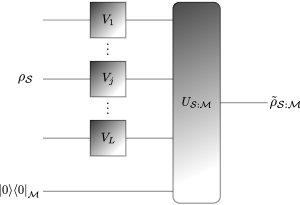
Figure 1: (Color online) Activation Protocol for an L-modes system.

Fig.1 pictures the activation protocol for an L-modes system, described by the density matrix $\rho_{S}\in\mathcal{D}(\mathcal{H}_{1}^{2}\otimes\cdots\otimes\mathcal{H}_{L}^{2})$, where the unitary operation $V_{j}$ represents rotation on mode $j$, and $U_{S:M}$ is a Cnot operation with the system as control and apparatus as target. The output state in the quantum circuit is:

$$\tilde{\rho}_{S:M}=U_{S:M}(V_{S}\otimes\mathbb{I}_{M})(\rho_{S}\otimes\mathopen{}\mathclose{{}\left|0\middle\rangle\middle\langle 0}\right|_{M})(V_{S}^{\dagger}\otimes\mathbb{I}_{M})U_{S:M}^{\dagger},$$

where $V_{S}=V_{1}\otimes\cdots\otimes V_{L}$. The post measurement state, resulted from the interaction between system and measurement apparatus is:

$$\tilde{\rho}_{S}=\sum_{\vec{l}}\hat{\Pi}_{\vec{l}}V_{S}\rho_{S}V_{S}^{\dagger}\hat{\Pi}_{\vec{l}},$$ (49)

with $\hat{\Pi}_{\vec{l}}=\hat{\Pi}_{l_{1}}\otimes\cdots\otimes\hat{\Pi}_{l_{L}}$. As aforementioned, the action of the unitary operation $V_{S}$ determines the projective measurement basis. Therefore, from Lemma 1, the unitary operation on each mode $j$ must preserve the symmetries of the state in order to minimize the local disturbance. Thus, for one-body systems with parity symmetry, there exists only one unitary operation $V_{j}=\mathbb{I}_{j}$ on each mode $j$. Therefore, the post measurement state, for one-body systems, is simply:

$$\tilde{\rho}_{S}=\sum_{\vec{l}}\hat{\Pi}_{\vec{l}}\rho_{S}\hat{\Pi}_{\vec{l}},$$ (50)

with $\hat{\Pi}_{l_{j}}=\{a_{j}^{\dagger}a_{j},a_{j}a_{j}^{\dagger}\}$ in a given representation of modes.

We will use the approach of activation protocol to discuss the classically correlated states. As shown in Ref.Piani et al. (2011), a quantum state $\chi$ is classically correlated if and only if there exists a unitary $V_{S}$ such that:

$$\chi_{S}=\tilde{\chi}_{S}=\sum_{\vec{l}}\hat{\Pi}_{\vec{l}}V_{S}\chi_{S}V_{S}^{\dagger}\hat{\Pi}_{\vec{l}},$$ (51)

which immediately holds for the activation protocol of $L$-modes represented in Fig.1. Actually, we can learn about the set of classically correlated states according to the one-body quantumness of particles, by means of the representation of modes. As the set of classically correlated states of particles satisfies $\mathcal{Q}_{sp}(\chi)=0$, for all $\chi$ in this set, there must exist an isomorphism $\Lambda:\mathcal{F}_{L}\leftrightarrow\mathcal{H}^{2\otimes L}$ of one-body particles such that $\sum_{j}\mathcal{Q}_{sp}^{(j)}(\chi)=0$. This equality holds if and only if:

$$\mathcal{Q}_{sp}^{(j)}(\chi)=0,\qquad\forall\,j=1,\cdots,N.$$

Therefore, for all $j$, there is a projective measurement $\Pi^{(j)}$ such that $\Pi^{(j)}(\chi)=\chi$. Thus a quantum state $\chi\in\mathcal{D}(\mathcal{F}_{L})$ is classically correlated, if and only if, there exist projective measurements in each mode $\Pi^{(1)}\otimes\cdots\otimes\Pi^{(L)}(\chi)=\chi$, such that

$$\chi=\sum_{\vec{l}}p(\vec{l})\hat{\Pi}_{l_{1}}\otimes\cdots\otimes\hat{\Pi}_{l_{L}},$$

where $\vec{l}=(l_{1},\ldots,l_{L})$ and $l_{j}=0,1$. From the definition of quantumness of correlations of particles in Eq.(33), and the isomorphism in Eq.(5), we can write the projectors as $\hat{\Pi}_{\vec{l}}=a_{1}^{l_{1}\dagger}\cdots a_{L}^{l_{L}\dagger}\mathopen{}\mathclose{{}\left|vac}\right\rangle\mathopen{}\mathclose{{}\left\langle vac}\right|a_{L}^{l_{L}}\cdots a_{1}^{l_{1}}$, and $\hat{\Pi}_{\vec{l}}=\hat{\Pi}_{l_{1}}\otimes\cdots\otimes\hat{\Pi}_{l_{L}}$, therefore the classically correlated states of particles can be written as:

$$\chi=\sum_{\vec{l}}p(\vec{l})a_{1}^{l_{1}\dagger}\cdots a_{L}^{l_{L}\dagger}\mathopen{}\mathclose{{}\left|vac}\right\rangle\mathopen{}\mathclose{{}\left\langle vac}\right|a_{L}^{l_{L}}\cdots a_{1}^{l_{1}}.$$ (52)

This results is in agreement with the set of classically correlated states obtained in Ref.Iemini et al. (2014), by means of the activation protocol Piani et al. (2011); Streltsov et al. (2011), for the zero way work deficit introduced in Eq.(26). As a matter of fact, as the set of classically correlated states of particles is independent of the isomorphism, we can write:

$$\mathcal{Q}_{p}^{\emptyset}(\chi)=\mathcal{Q}_{sp}(\chi)=0.$$ (53)

It is important to note that the classicality of correlations of particles, for a given state, does not imply in a classically correlated state for a given mode representation. In other words, the system of particles can be classically correlated, whereas there exist modes that are quantum correlated. The requirement, for the particles be classically correlated, in Eq.(33) is the existence of at least one representation $\Lambda:\mathcal{F}_{L}\leftrightarrow\mathcal{H}^{2\otimes L}$ such that the modes are classically correlated Zanardi (2001).

VI Dissipative System

In this section, we study a physical system and its quantumness of correlations in order to illustrate the previous discussions. We investigate a purely dissipative system, whose stationary states exhibit interesting topological non-local correlations. The motivation for the study of a dissipative system stems from the fact that its dynamics tends to mix the quantum state, allowing us to study the quantumness of correlations beyond entanglement, since for pure states such notions usually overlap. Furthermore, we consider a system which conserves the total number of particles, as we will describe in more detail later, and in this way we can use our previous results for the quantumness of symmetric states. Let us give a brief overview of dynamics in open systems and present the physical setting under scrutiny.

In general, evolutions in dissipative open quantum systems tend to annihilate the quantum correlations present in the system, leading to steady states described by trivial mixed states. There are cases, however, in which the many-body density matrix is driven towards a pure steady state, $\rho_{f}=\mathopen{}\mathclose{{}\left|\psi_{D}\middle\rangle\middle\langle\psi_{D}}\right|$, commonly called as dark states in quantum optics. Recently, theoretical and experimental studies Iemini et al. (2016); Diehl et al. (2008); Verstraete et al. (2009); Diehl et al. (2011) have focused on how to properly engineer the environment such that, in the long-time limit, it drives the system into certain desired quantum states. In particular, we study here the dissipative number conserving system as proposed in Iemini et al. (2016), consisting of a single, or two-leg ladder, properly coupled to the environment. It was shown that such setup leads to topological superconductors as steady states, exhibiting non-local edge correlation and Majorana zero modes, with promising applications for topologically protected quantum memory and computing Nayak et al. (2008).

Let us formally describe the system we will study. The time evolution of a system coupled to a Markovian reservoir (memoryless reservoir) is described by a master equation, cast in the following form,

$$\frac{\partial\rho}{\partial t}=\hat{\mathcal{L}}[\rho]=-i\,\mathopen{}\mathclose{{}\left[\hat{H},\rho}\right]+J\sum_{j}\mathopen{}\mathclose{{}\left(\hat{L}_{j}\rho\hat{L}^{\dagger}_{j}-\frac{1}{2}\mathopen{}\mathclose{{}\left\{\hat{L}^{\dagger}_{j}\hat{L}_{j},\rho}\right\}}\right),$$

(54)

where $\rho$ is the density matrix, $\hat{\mathcal{L}}$ is the Liouvillian of the evolution, $\hat{H}$ is the Hamiltonian of the system, and $\hat{L}_{j}$ are the Lindblad operators. Considering a purely dissipative evolution ($\hat{H}=0$), possible pure dark states in the system are mathematically related to zero modes of the Liouville operator. More precisely, dark states are zero modes shared by all Lindblad operators:

$$\hat{L}_{j}\mathopen{}\mathclose{{}\left|\psi_{D}}\right\rangle=0,\quad\forall j.$$ (55)

Their existence, however, is not always guaranteed. We study a one-dimensional fermionic system with $L$ sites, evolved by the following number-conserving Lindblad operators:

$$\hat{L}_{j}=(a^{\dagger}_{j}+a^{\dagger}_{j+1})(a_{j}-a_{j+1}),$$ (56)

where $a^{(\dagger)}_{j}$ are the fermionic annihilation (creation) operators at the site $j$, and we consider open boundary conditions ($j=1,...,L-1$). In this setting, the dark states are $p$-wave superconductors with fixed number of particles.

Let us focus now in the simpler non-trivial fermionic system which can present quantum correlations beyond the mere exchange statistics, i.e., a system with $L=4$ sites and $N=2$ particles. Even for such a small setting, the dissipative system is already able to create superconducting correlations between the particles. Interestingly, the exact expression for such steady state in real space was studied not only in the realm of dissipative systems Iemini et al. (2016), but also as ground states of a closed Hamiltonian Iemini et al. (2015b), and is given by the equal weighted superposition of all possible configurations of its $N$ particles in the $L$ sites; precisely,

$$\mathopen{}\mathclose{{}\left|\psi_{D}}\right\rangle=\frac{\mathopen{}\mathclose{{}\left(a^{\dagger}_{1}a^{\dagger}_{2}+a^{\dagger}_{1}a^{\dagger}_{3}+a^{\dagger}_{1}a^{\dagger}_{4}+a^{\dagger}_{2}a^{\dagger}_{3}+a^{\dagger}_{2}a^{\dagger}_{4}+a^{\dagger}_{3}a^{\dagger}_{4}}\right)}{\sqrt{6}}\mathopen{}\mathclose{{}\left|vac}\right\rangle.$$

Since the above setting conserves the total number of particles, we can use our results for the quantumness in symmetric states. Thus, we study the dynamics for an initial uncorrelated single-Slater determinant state,

$$\mathopen{}\mathclose{{}\left|\psi(t=0)}\right\rangle=a^{\dagger}_{1}a^{\dagger}_{3}\mathopen{}\mathclose{{}\left|vac}\right\rangle.$$ (57)

In order to characterize the time evolution described by the master equation (Eq.(54)), we use the Runge-Kutta integration. This method entails an error due to inaccuracies in the numerical integration, but the full density matrix is represented without any approximation.

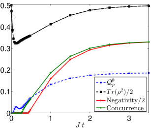
Figure 2: (Color online) Dissipative evolution for a system with $L=4$ sites and $N=2$ particles, considering an initially uncorrelated single-Slater determinant state (Eq.(57)). We show the time evolution for the quantumness of correlation of the state ($\mathcal{Q}_{p}^{\emptyset}$), its purity ($\text{Tr}(\rho^{2})$) and its entanglement according to the Shifted Negativity Iemini and Vianna (2013) and Concurrence Eckert et al. (2002) quantifiers.

We present our numerical simulation in Fig.(2). At the early stages of the evolution, the quantum state becomes highly mixed, and we already see the creation of quantumness between its particles. Already in the beginning of the evolution, $tJ\ll 1$, several excited modes of the Liouvillian have non-trivial effects in the dynamics, and in this way the observables present fast oscillations in this regime. For longer times, only the first excited states of the Liouvillian have non-trivial effects in the evolution, and the dynamical behavior becomes smoother. We see that the quantum state is driven, exponentially fast in time, to a pure state with non-trivial quantumness of correlations, as expected from the previous discussions. Interesting to notice that the quantumness for the steady state agrees with the entanglement entropy for indistinguishable particles Iemini and Vianna (2013), i.e., $\mathcal{Q}^{\emptyset}_{p}(\mathopen{}\mathclose{{}\left|\psi\middle\rangle\middle\langle\psi}\right|_{D})=S(\mathopen{}\mathclose{{}\left|\psi\middle\rangle\middle\langle\psi}\right|_{D})-\ln N$.

To exemplify the different nature of the quantumness of correlations to the entanglement of particles, we also plot the entanglement dynamics according to some usual quantifiers in the literature. Precisely, we compare the quantumness of correlations to the Shifted Negativity Iemini and Vianna (2013) and Concurrence Eckert et al. (2002). It it very clear the more general character of the quantumness of correlation, showing a richer dynamics for the initial evolution, while there is absolutely no entanglement in the state. We can also notice that the state has bound entanglement, analogous to the positive partial transpose (PPT) entangled states in distinguishable systems, for values of $Jt\in[0.3,0.45]$, as the negativity is null, besides the concurrence has non zero values.

VII Local Projectors Structure - Numerical Results

In this section we analyze, numerically, the quantumness of more general symmetric quantum states and their respective local projectors, as given in Definition 1. Our motivations here are two-fold: (i) to analyze if there are other solutions for the local projectors in Lemma 1, i.e., solutions which do not share the quantum state symmetry; (ii) to analyze if Lemma 1 could be extended for general states with parity symmetry, $[\rho,(-1)^{\hat{N}}]=0$, beyond the restriction to a single symmetry eigenvalue.

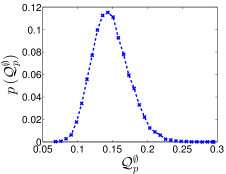
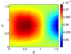
Figure 3: (Color online) On the left, we show the probability distribution for the quantumness of correlations in the sampled space to $E_{par}$. We use a sample space of $\sim 10^{5}$ quantum states. In the middle (on the right) we show the $T_{E}(\phi,\theta)$ function for the $E_{par}^{(1)}$ ($E_{par}$) ensemble.

We focus on a simple bipartite case, formed by a single particle mode ($1$ qubit) and the other $L-1$ modes. In this case, we can parametrize the local projectors in the single particle mode subspace with only two parameters, $\{\phi,\theta\}$. Since the projectors are rank-$1$, we need to parametrize only two orthogonal pure states in such subspace, as follows,

$$\mathopen{}\mathclose{{}\left|\psi_{1}(\phi,\theta)}\right\rangle = \cos(\phi)\mathopen{}\mathclose{{}\left|0}\right\rangle+e^{i\theta}\sin(\phi)\mathopen{}\mathclose{{}\left|1}\right\rangle$$ (58)

$$\mathopen{}\mathclose{{}\left|\psi_{2}(\phi,\theta)}\right\rangle = -e^{-i\theta}\sin(\phi)\mathopen{}\mathclose{{}\left|0}\right\rangle+\cos(\phi)\mathopen{}\mathclose{{}\left|1}\right\rangle;$$ (59)

where $\mathopen{}\mathclose{{}\left|1}\right\rangle$ ($\mathopen{}\mathclose{{}\left|0}\right\rangle$) is the state with one (no) fermion occupying the single particle mode, $0\leq\phi\leq\pi$ and $0\leq\theta<2\pi$. The local projectors are thus defined as $\Pi_{1(2)}^{(\phi,\theta)}=\mathopen{}\mathclose{{}\left|\psi_{1(2)}(\phi,\theta)\middle\rangle\middle\langle\psi_{1(2)}(\phi,\theta)}\right|$. We define now the function $T_{E}(\phi,\theta)$ for such projectors as,

$$T_{E}(\phi,\theta)=\int_{\rho\in E}\mathopen{}\mathclose{{}\left\{S(\rho||{\Pi}^{(\phi,\theta)}[\rho])-\mathcal{Q}_{p}^{\emptyset}(\rho)}\right\}d\rho,$$ (60)

where ${\Pi}^{(\phi,\theta)}[\rho]=\hat{\Pi}_{1}^{\phi,\theta}\rho\hat{\Pi}_{1}^{\phi,\theta}+\hat{\Pi}_{2}^{\phi,\theta}\rho\hat{\Pi}_{2}^{\phi,\theta}$, and the integral is taken over an ensemble $E$ of quantum states. The above function gives us a notion of an effective perturbation - in comparison to the minimum one - of the local projectors onto the corresponding ensemble $E$.

We consider an ensemble $E_{par}$ with parity symmetry, $[\rho,(-1)^{\hat{N}}]=0,$ $\forall\rho\in E_{par}$, and a subset $E_{par}^{(1)}$ thereof, whose quantum states have a single eigenvalue of the parity symmetry. This latter case - $E_{par}^{(1)}$ - corresponds to the conditions of Lemma 1.

The integration of Eq.(60) is performed over a sample of quantum states ($\sim 10^{5}$ states) approximating the corresponding ensemble. The sample is chosen according to the Haar measure. On the left of Fig.(3), we plot the probability distribution for the quantumness of correlations of the sampled space corresponding to the $E_{par}$ ensemble.

Let us now analyze the $T_{E}(\phi,\theta)$ function for the $E_{par}^{(1)}$ and $E_{par}$ ensembles. In the former case (middle of Fig.(3)) we obtained that $T(\phi,\theta)=0$ $\iff$ $\phi=0,\pi/2$ (we omit here $\phi>\pi/2$ for symmetry reasons), which corresponds to the projectors with the shared symmetry, as expected from our Lemma. It was also observed in our simulations that $S(\rho||{\Pi}^{(\phi,\theta)}[\rho])-\mathcal{Q}(\rho)=0$ $\iff$ $\phi=0,\pi/2$, confirming that the only optimal projectors are indeed those of the Lemma. On the right of Fig.(3), we show our results for the more general ensemble $E_{par}$. We see now that the Lemma cannot be extended for such ensemble. We also see that there is no set of symmetric local projectors minimizing the local disturbance. The analysis of the quantumness of correlations in these cases demands a more careful treatment.

VIII Conclusion

In this work we proposed a new description for the quantification of quantumness of correlations in fermionic systems. We proved in Lemma 1 that the symmetries of a state can improve the optimization of the local disturbance, once that the optimal local projective measurement is also symmetric. As discussed, it holds for symmetric states with a single eigenvalue of the symmetry operator. Numerical evidences suggest the uniqueness of the symmetric solution for the minimal local disturbance, as well as the impossibility of extending the Lemma 1 for states with multiple eigenvalues of the symmetry operator. In Theorem 1, we restrict our discussion for states with parity symmetry, showing that the minimization of the multipartite relative entropy of quantumness reduces to the notion of quantumness of correlations of indistinguishable particles. By means of the activation protocol, we have also characterized the class of fermionic states without quantumness of correlations. We illustrated our results with the dynamics of quantumness of correlations for a purely dissipative system of two particles and four sites. Our results shed new light and give fresh perspectives on the characterization and quantification of quantum correlations in fermionic systems.

Appendix - Proof of Lemma 1

Proof.

Consider a symmetry $\Theta$ with $N$ degenerate eigenvalues $\{\theta_{j}\}_{j=1}^{N}$. In its eigenbasis, it can be written as:

$$\Theta=\begin{pmatrix}\hat{\theta}_{1}&\cdots&0\\ 0&\ddots&0\\ 0&\cdots&\hat{\theta}_{N}\end{pmatrix},$$ (61)

where $\hat{\theta}_{j}$ are $n_{j}\times n_{j}$ matrices, with $n_{j}$ being the degeneracy of eigenvalue $\theta_{j}$. The observable $\Theta$ acts on a D-dimensional Hilbert space $\mathcal{H}^{D}$, where $D=\sum_{j=1}^{N}n_{j}$.

A given state $\rho_{j}$ has a symmetry over an eigenvalue $\theta_{j}$ if $[\rho_{j},\hat{\theta}_{j}]=0$. Therefore, a system described by a density matrix $\rho_{S}\in\mathcal{D}(\mathcal{H}_{S})$ has the symmetry $\Theta$, if the density matrix can be written as a convex combination of the set of $\rho_{j}$ for all eigenvalues $\theta_{j}$, namely:

$$\rho_{S}=\sum_{j}q_{j}\rho_{j}.$$

Thus there exists an isometry $V_{X}:\mathcal{H}_{S}\rightarrow\mathcal{H}_{S}\otimes\mathcal{H}_{X}$, which acts on the eigenbasis of $\Theta$ as:

$$V_{X}\mathopen{}\mathclose{{}\left|\theta_{j}(l)}\right\rangle_{S}=\mathopen{}\mathclose{{}\left|\theta_{j}(l)}\right\rangle_{S}\mathopen{}\mathclose{{}\left|\theta_{j}}\right\rangle_{X},$$

where $\{\mathopen{}\mathclose{{}\left|\theta_{j}(l)}\right\rangle_{S}\}_{l=1}^{n_{j}}$ are the eigenvectors related to the eigenvalue $\theta_{j}$. $\mathcal{H}_{S}$ is the Hilbert space of the system, and $\mathcal{H}_{X}$ is an ancillary space such that $\text{dim}(\mathcal{H}_{S})\times\text{dim}(\mathcal{H}_{X})=D$. Therefore, the action of the isometry over the symmetric density matrix $\rho_{S}$ is:

$$\rho_{SX}=V_{X}\rho_{S}V_{X}^{\dagger}=\sum_{j}q_{j}\rho^{S}_{j}\otimes\mathopen{}\mathclose{{}\left|\theta_{j}\middle\rangle\middle\langle\theta_{j}}\right|_{X},$$

which is a block diagonal matrix, with the blocks labeled by the eigenvalues of $\Theta$, and consequently $[\rho_{SX},\Theta]=0$. The set $\{\mathopen{}\mathclose{{}\left|\theta_{j}}\right\rangle\}_{j=1}^{N}$ is an orthonormal basis on $\mathcal{H}_{X}$. Each density matrix $\rho_{j}^{S}$ acts on the space spanned by the eigenvectors of the eigenvalue $\theta_{j}$.

We separate the projective measurements over a symmetric state in two kinds: with and without the symmetry. To represent these two different measurements we use the approach of an enlarged state space, described below. The way that the measurement acts over the space $\mathcal{H}_{X}$ defines if it has or has not the symmetry. A projective measurement with the symmetry must keep the block diagonal form of the density matrix, respecting the label on the eigenvalues of $\Theta$ described by the basis $\{\mathopen{}\mathclose{{}\left|\theta_{j}}\right\rangle\}_{j}$ on $\mathcal{H}_{X}$. On the other hand, a projective measurement without the symmetry will create overlap with this same basis, destroying the symmetry and the block diagonal structure of the density matrix in the enlarged space. In the case of a modes partitioning, the Hilbert space of the system is composed as $\mathcal{H}_{S}=\mathcal{H}_{A}\otimes\mathcal{H}_{B}$. Thus to prove the Lemma, we define two local projective measurement maps: a $\mathcal{P}^{\theta}_{BX}$ that has the symmetry on $\Theta$, and a map $\Pi_{BX}$ without the symmetry. We obtain the proof of the Lemma by showing that the local disturbance, created on $\rho_{ABX}$ by $\mathcal{P}^{\theta}_{BX}$, is smaller than that crated by $\Pi_{BX}$, for a state with symmetry over one eigenvalue $\theta_{j}$:

$$S(\rho_{ABX}||\mathcal{P}^{\theta}_{BX}(\rho_{ABX}))\leq S(\rho_{ABX}||\Pi_{BX}(\rho_{ABX})).$$ (62)

As $\mathcal{P}^{\theta}_{BX}$ has the symmetry over the eigenvalues of $\Theta$, it must act on $\rho_{ABX}=\sum_{j}q_{j}\rho^{AB}_{j}\otimes\mathopen{}\mathclose{{}\left|\theta_{j}\middle\rangle\middle\langle\theta_{j}}\right|_{X}$ inside the blocks:

$$\mathcal{P}^{\theta}_{BX}(\rho_{ABX})=\begin{pmatrix}q_{1}\mathcal{P}_{B}(\rho^{AB}_{1})&\cdots&0\\ 0&\ddots&0\\ 0&\cdots&q_{N}\mathcal{P}_{B}(\rho^{AB}_{N})\end{pmatrix},$$ (63)

where $\mathcal{P}_{B}(\rho^{AB}_{j})$ is a local projective measurement over subsystem $B$. For the projective measurement to satisfy Eq.(63), the projectors must be in the form:

$$P_{b,x}=P_{b}^{B}\otimes\mathopen{}\mathclose{{}\left|\theta_{x}\middle\rangle\middle\langle\theta_{x}}\right|_{X}.$$

Then its action over $\rho_{ABX}$ respects:

$$\mathcal{P}^{\theta}_{BX}(\rho_{ABX})=\sum_{j}q_{j}\mathbb{P}_{B}(\rho^{AB}_{j})\otimes{\theta_{j}}_{X},$$

where $\mathbb{P}_{B}(\rho^{AB}_{j})$ is a local projective measurement map over subsystem $B$, with projectors $\{P_{b}\}$, as presented in Eq.(9). For the disturbance created by this measurement, we can write:

$$S(\rho_{ABX}||\mathcal{P}^{\theta}_{BX}(\rho_{ABX}))=\sum_{j}q_{j}S(\rho^{AB}_{j}||\mathbb{P}_{B}(\rho^{AB}_{j})),$$

once that $S(\sum_{x}p_{x}\mathopen{}\mathclose{{}\left|x\middle\rangle\middle\langle x}\right|\otimes\rho_{x}||\sum_{x}p_{x}\mathopen{}\mathclose{{}\left|x\middle\rangle\middle\langle x}\right|\otimes\sigma_{x})=\sum_{x}p_{x}S(\rho_{x}||\sigma_{x})$. On the other hand, the projective measurement $\Pi_{BX}$ creates an overlap on the orthonormal basis $\{\mathopen{}\mathclose{{}\left|\theta_{j}}\right\rangle\}$. It must act over space $B$ and $X$ locally, without creating correlations between them, however creating overlap between the basis $\mathopen{}\mathclose{{}\left|\theta_{j}}\right\rangle$ and another basis in $\mathcal{H}_{X}$. We have:

$$\Pi_{b,x}=\Pi_{b}\otimes\mathopen{}\mathclose{{}\left|x\middle\rangle\middle\langle x}\right|_{X},$$ (64)

for $\{\mathopen{}\mathclose{{}\left|x}\right\rangle\}$ an orthonormal basis in $\mathcal{H}_{X}$, thus the action of the map can be written as:

$$\Pi_{BX}(\rho_{ABX})=\sum_{j}q_{j}\sum_{x}p(x|j){\Pi}_{B}(\rho_{j}^{AB})\otimes\mathopen{}\mathclose{{}\left|x\middle\rangle\middle\langle x}\right|_{X},$$

where $p(x|j)=|\mathopen{}\mathclose{{}\left\langle x\middle|\theta_{j}}\right\rangle|^{2}$ represents the overlap between the eigenstates of $\Theta$ under the action of the projective measurement. As the relative entropy decreases under the partial trace operation, then tracing over subsystem $X$, the local disturbance created by $\Pi_{BX}$ satisfies:

$$S(\rho_{ABX}||\Pi_{BX}(\rho_{ABX}))\geq S(\sum_{j}q_{j}\rho_{j}^{AB}||\sum_{j}q_{j}{\Pi}_{B}(\rho_{j}^{AB})),$$

with $\sum_{x}p(x|j)=1$ and $\text{Tr}_{X}(\rho_{ABX})=\sum_{j}q_{j}\rho_{j}^{AB}$.

Therefore, considering a bipartite state $\rho_{l}^{AB}$ with symmetry in only one eigenvalue $\theta_{l}$ of $\Theta$, there exists just one term in the sum $\sum_{j}q_{j}\delta_{j,l}=q_{l}=1$, which implies $\rho_{ABX}=\rho_{l}^{AB}\otimes\mathopen{}\mathclose{{}\left|\theta_{l}\middle\rangle\middle\langle\theta_{l}}\right|_{X}$, and the disturbances satisfy:

$$S(\rho_{ABX}||\mathcal{P}^{\theta}_{BX}(\rho_{ABX}))=S(\rho^{AB}_{l}||\mathbb{P}_{B}(\rho^{AB}_{l})),$$ (65)

and

$$S(\rho_{ABX}||\Pi_{BX}(\rho_{ABX}))\geq S(\rho_{l}^{AB}||{\Pi}_{B}(\rho_{l}^{AB})).$$ (66)

The optimization in the one-way work deficit is taken over all projective measurements that act over subspace $B$. Therefore, as ${\Pi}_{B}(\rho_{l}^{AB})$ and $\mathbb{P}_{B}(\rho^{AB}_{l})$ are restricted by the symmetry to act on this same space, and the state has null projection on any other subspace of the symmetry, the smallest local disturbance created by these two projective measurement can attain the same value:

$$\min_{\mathbb{P}_{B}}S(\rho^{AB}_{l}||\mathbb{P}_{B}(\rho^{AB}_{l}))=\min_{{\Pi}_{B}}S(\rho_{l}^{AB}||{\Pi}_{B}(\rho_{l}^{AB})).$$

Finally,by Eq.(65) and Eq.(66), we obtain:

$$S(\rho_{ABX}||\mathcal{P}^{\theta}_{BX}(\rho_{ABX}))\leq S(\rho_{ABX}||\Pi_{BX}(\rho_{ABX})),$$

which means that local projective measurements, with the symmetry of the state, create less disturbance than local projective measurements without the symmetry, proving the Lemma.

Besides the proof was performed for bipartite systems, it also holds for multipartite systems, simply generalizing the projective measurements over partition $B$ to multipartite projectors. ∎

References

- Nielsen and Chuang (2010) M. A. Nielsen and I. L. Chuang, Quantum computation and quantum information (Cambridge university press, 2010).
- Nayak et al. (2008) C. Nayak, S. H. Simon, A. Stern, M. Freedman, and S. D. Sarma, Rev. Mod. Phys. 80, 1083 (2008).
- Zanardi (2002) P. Zanardi, Physical Review A 65, 042101 (2002).
- Wiseman and Vaccaro (2003) H. M. Wiseman and J. A. Vaccaro, Physical review letters 91, 097902 (2003).
- Eckert et al. (2002) K. Eckert, J. Schliemann, D. Bruss, and M. Lewenstein, Annals of Physics 299, 88 (2002).
- Amico et al. (2008) L. Amico, R. Fazio, A. Osterloh, and V. Vedral, Reviews of Modern Physics 80, 517 (2008).
- Iemini et al. (2015a) F. Iemini, T. O. Maciel, and R. O. Vianna, Phys. Rev. B 92, 075423 (2015a), URL http://link.aps.org/doi/10.1103/PhysRevB.92.075423.
- Friis et al. (2013) N. Friis, A. R. Lee, and D. E. Bruschi, Physical Review A 87, 022338 (2013).
- Balachandran et al. (2013) A. P. Balachandran, T. R. Govindarajan, A. R. de Queiroz, and A. F. Reyes-Lega, Phys. Rev. Lett. 110, 080503 (2013), URL http://link.aps.org/doi/10.1103/PhysRevLett.110.080503.
- Iemini et al. (2013) F. Iemini, T. O. Maciel, T. Debarba, and R. O. Vianna, Quantum Information Processing 12, 733 (2013), ISSN 1573-1332, URL http://dx.doi.org/10.1007/s11128-012-0415-6.
- Iemini and Vianna (2013) F. Iemini and R. O. Vianna, Phys. Rev. A 87, 022327 (2013), URL http://link.aps.org/doi/10.1103/PhysRevA.87.022327.
- Henderson and Vedral (2001) L. Henderson and V. Vedral, Journal of Physics A: Mathematical and General 34, 6899 (2001), URL http://stacks.iop.org/0305-4470/34/i=35/a=315.
- Ollivier and Zurek (2001) H. Ollivier and W. H. Zurek, Phys. Rev. Lett. 88, 017901 (2001), URL http://link.aps.org/doi/10.1103/PhysRevLett.88.017901.
- Modi et al. (2010) K. Modi, T. Paterek, W. Son, V. Vedral, and M. Williamson, Phys. Rev. Lett. 104, 080501 (2010).
- Debarba et al. (2012) T. Debarba, T. O. Maciel, and R. O. Vianna, Phys. Rev. A 86, 024302 (2012).
- Iemini et al. (2014) F. Iemini, T. Debarba, and R. O. Vianna, Phys. Rev. A 89, 032324 (2014), URL http://link.aps.org/doi/10.1103/PhysRevA.89.032324.
- Piani et al. (2011) M. Piani, S. Gharibian, G. Adesso, J. Calsamiglia, P. Horodecki, and A. Winter, Phys. Rev. Lett. 106, 220403 (2011), URL http://link.aps.org/doi/10.1103/PhysRevLett.106.220403.
- Streltsov et al. (2011) A. Streltsov, H. Kampermann, and D. Bruß, Physical review letters 106, 160401 (2011), URL http://prl.aps.org/pdf/PRL/v106/i16/e160401.
- Benatti et al. (2010) F. Benatti, R. Floreanini, and U. Marzolino, Annals of Physics 325, 924 (2010).
- Bañuls et al. (2007) M.-C. Bañuls, J. I. Cirac, and M. M. Wolf, Physical Review A 76, 022311 (2007).
- Brodutch and Modi (2012) A. Brodutch and K. Modi, Quantum Information & Computation 12, 721 (2012).
- Luo (2008) S. Luo, Phys. Rev. A 77, 022301 (2008), URL http://link.aps.org/doi/10.1103/PhysRevA.77.022301.
- Nakano et al. (2012) T. Nakano, M. Piani, and G. Adesso (2012), eprint 1211.4022v1, URL http://arxiv.org/abs/1211.4022v1.
- Oppenheim et al. (2002) J. Oppenheim, M. Horodecki, P. Horodecki, and R. Horodecki, Phys. Rev. Lett. 89, 180402 (2002), URL http://link.aps.org/doi/10.1103/PhysRevLett.89.180402.
- Horodecki et al. (2005) M. Horodecki, P. Horodecki, R. Horodecki, J. Oppenheim, A. De, U. Sen, and B. Synak-Radtke, Physical Review A 71, 062307 (2005).
- Ban et al. (1997) M. Ban, K. Kurokawa, R. Momose, and O. Hirota, International Journal of Theoretical Physics 36, 1269 (1997).
- Sasaki et al. (1999) M. Sasaki, S. M. Barnett, R. Jozsa, M. Osaki, and O. Hirota, Physical Review A 59, 3325 (1999), URL http://arxiv.org/pdf/quant-ph/9812062.pdf.
- Davies (1978) E. Davies, Information Theory, IEEE Transactions on 24, 596 (1978).
- Chiribella and Mauro D’Ariano (2006) G. Chiribella and G. Mauro D’Ariano, Journal of Mathematical Physics 47, 092107 (2006), URL http://scitation.aip.org/content/aip/journal/jmp/47/9/10.1063/1.2349481.
- Gigena and Rossignoli (2015) N. Gigena and R. Rossignoli, Phys. Rev. A 92, 042326 (2015), URL http://link.aps.org/doi/10.1103/PhysRevA.92.042326.
- Gigena and Rossignoli (2016) N. Gigena and R. Rossignoli, Physical Review A 94, 042315 (2016).
- Zanardi (2001) P. Zanardi, Phys. Rev. Lett. 87, 077901 (2001), URL http://link.aps.org/doi/10.1103/PhysRevLett.87.077901.
- Iemini et al. (2016) F. Iemini, D. Rossini, R. Fazio, S. Diehl, and L. Mazza, Phys. Rev. B 93, 115113 (2016), URL http://link.aps.org/doi/10.1103/PhysRevB.93.115113.
- Diehl et al. (2008) S. Diehl, A. Micheli, A. Kantian, B. Kraus, H. Buchler, and P. Zoller, Nature Phys. 4, 878 (2008).
- Verstraete et al. (2009) F. Verstraete, M. M. Wolf, and J. I. Cirac, Nature Phys. 5, 633 (2009).
- Diehl et al. (2011) S. Diehl, E. Rico, M. Baranov, and P. Zoller, Nature Phys. 7, 971 (2011).
- Iemini et al. (2015b) F. Iemini, L. Mazza, D. Rossini, R. Fazio, and S. Diehl, Phys. Rev. Lett. 115, 156402 (2015b), URL http://link.aps.org/doi/10.1103/PhysRevLett.115.156402.