Estimating the marginal likelihood with Integrated nested Laplace approximation (INLA)

Abstract

The marginal likelihood is a well established model selection criterion in Bayesian statistics. It also allows to efficiently calculate the marginal posterior model probabilities that can be used for Bayesian model averaging of quantities of interest. For many complex models, including latent modeling approaches, marginal likelihoods are however difficult to compute. One recent promising approach for approximating the marginal likelihood is Integrated Nested Laplace Approximation (INLA), design for models with latent Gaussian structures. In this study we compare the approximations obtained with INLA to some alternative approaches on a number of examples of different complexity. In particular we address a simple linear latent model, a Bayesian linear regression model, logistic Bayesian regression models with probit and logit links, and a Poisson longitudinal generalized linear mixed model.

Keywords: Integrated nested Laplace approximation; Marginal likelihood; Model Evidence; Bayes Factor; Markov chain Monte Carlo; Numerical Integration; Linear models; Generalized linear models; Generalized linear mixed models; Bayesian model selection; Bayesian model averaging.

1 Introduction

Marginal likelihoods have been commonly accepted to be an extremely important quantity within Bayesian statistics. For data $\mathbf{y}$ and model $\mathcal{M}$, which includes some unknown parameters $\theta$, the marginal likelihood is given by

$$p(\mathbf{y}|\mathcal{M})=\int_{\Omega_{\theta}}p(\mathbf{y}|\mathcal{M},\theta)p(\theta|\mathcal{M})d\theta$$ (1)

where $p(\theta|\mathcal{M})$ is the prior for $\theta$ under model $\mathcal{M}$ while $p(\mathbf{y}|\mathcal{M},\theta)$ is the likelihood function conditional on $\theta$. Consider first the problem of comparing models $\mathcal{M}_{i}$ and $\mathcal{M}_{j}$ through the ratio between their posterior probabilities:

$$\frac{p(\mathcal{M}_{i}|\mathbf{y})}{p(\mathcal{M}_{j}|\mathbf{y})}=\frac{p(\mathbf{y}|\mathcal{M}_{i})}{p(\mathbf{y}|\mathcal{M}_{j})}\times\frac{p(\mathcal{M}_{i})}{p(\mathcal{M}_{j})}.$$ (2)

The first term of the right hand side is the Bayes Factor (Kass and Raftery, 1995). In this way one usually performs Bayesian model selection with respect to the posterior marginal model model probabilities without the need to calculate them explicitly. However if we are interested in Bayesian model averaging and marginalizing some quantity $\Delta$ over the given set of models $\Omega_{\mathcal{M}}$ we are calculating the posterior marginal distribution, which in our notation becomes:

$$p(\Delta|\mathbf{y})=\sum_{\mathcal{M}\in\Omega_{\mathcal{M}}}{p(\Delta|\mathcal{M},\mathbf{y})p(\mathcal{M}|\mathbf{y})}.$$ (3)

Here $p(\mathcal{M}|\mathbf{y})$ is the posterior marginal model probability for model $\mathcal{M}$ that can be calculated with respect to Bayes theorem as:

$$p(\mathcal{M}|\mathbf{y})=\frac{{p(\mathbf{y}|\mathcal{M})p(\mathcal{M})}}{\sum_{\boldsymbol{\mathcal{M}}^{\prime}\in\Omega_{\mathcal{M}}}{p(\mathbf{y}|\mathcal{M}^{\prime})p(\mathcal{M}^{\prime})}},$$ (4)

Thus one requires marginal likelihoods $p(\mathbf{y}|\mathcal{M})$ in (2), (3) and (4). Metropolis-Hastings algorithms searching through models within a Monte Carlo setting (e.g. Hubin and Storvik, 2016) requires acceptance ratios of the form

$$r_{m}({\mathcal{M}},\mathcal{M}^{*})=\min\left\{1,\frac{p(\mathbf{y}|\mathcal{M}^{*})p(\mathcal{M}^{*})q({\mathcal{M}}|\mathcal{M}^{*})}{p(\mathbf{y}|\mathcal{M})p(\mathcal{M})q(\mathcal{M}^{*}|{\mathcal{M}})}\right\}$$ (5)

also involving the marginal likelihoods. All these examples show the fundamental importance of being able to calculate marginal likelihoods $p(\mathbf{y}|\mathcal{M})$ in Bayesian statistics.

Unfortunately for most of the models that include both unknown parameters $\theta$ and some latent variables $\boldsymbol{\eta}$ analytical calculation of $p(\mathbf{y}|\mathcal{M})$ is impossible. In such situations one must use approximative methods that hopefully are accurate enough to neglect the approximation errors involved. Different approximative approaches have been mentioned in various settings of Bayesian variable selection and Bayesian model averaging. Laplace’s method (Tierney and Kadane, 1986) has been widely used, but it is based on rather strong assumptions. The Harmonic mean estimator (Newton and Raftery, 1994) is an easy to implement MCMC based method, but it can give high variability in the estimates. Chib’s method (Chib, 1995), and its extension (Chib and Jeliazkov, 2001), are also MCMC based approaches that have gained increasing popularity. They can be very accurate provided enough MCMC iterations are performed, but need to be adopted to each application and the specific algorithm used. Approximate Bayesian Computation (ABC, Marin et al., 2012) has also been considered in this context, being much faster than MCMC alternatives, but also giving cruder approximations. Variational methods (Jordan et al., 1999) provide lower bounds for the marginal likelihoods and have been used for model selection in e.g. mixture models (McGrory and Titterington, 2007). Integrated nested Laplace approximation (INLA, Rue et al., 2009) provides estimates of marginal likelihoods within the class of latent Gaussian models and has become extremely popular. The reason for it is that Bayesian inference within INLA is extremely fast and remains at the same time reasonably precise.

Friel and Wyse (2012) perform comparison of some of the mentioned approaches including Laplace approximations, harmonic mean approximations, Chib’s method and other. However to our awareness there were no studies comparing the approximations of the marginal likelihood obtained by INLA with other popular methods mentioned in this paragraph. Hence the main goal of this article is to explore the precision of INLA in comparison with the mentioned above alternatives. INLA approximates marginal likelihoods by

$$p(\mathbf{y}|\mathcal{M})\approx\int_{\Omega_{\theta}}\left.\frac{p(\mathbf{y},\theta,\boldsymbol{\eta}|\mathcal{M})}{\tilde{\pi}_{G}(\boldsymbol{\eta}|\mathbf{y},\theta,\mathcal{M})}\right\rvert_{\boldsymbol{\eta}=\boldsymbol{\eta}^{*}(\theta|\mathcal{M})}d\theta,$$ (6)

where $\boldsymbol{\eta}^{*}(\theta|\mathcal{M})$ is some chosen value of $\boldsymbol{\eta}$, typically the posterior mode, while $\tilde{\pi}_{G}(\boldsymbol{\eta}|\mathbf{y},\theta,\mathcal{M})$ is a Gaussian approximation to $\pi(\boldsymbol{\eta}|\mathbf{y},\theta,\mathcal{M})$. Within the INLA framework both random effects and regression parameters are treated as latent variables, making the dimension of the hyperparmeters $\theta$ typically low. The integration of $\theta$ over the support ${\Omega_{\theta}}$ can be performed by an empirical Bayes (EB) approximation or using numerical integration based on a central composite design (CCD) or a grid (see Rue et al., 2009, for details).

In the following sections we will evaluate the performance of INLA through a number of examples of different complexities, beginning with a simple linear latent model and ending up with a Poisson longitudinal generalized linear mixed model.

2 INLA versus truth and the harmonic mean

To begin with we address an extremely simple example suggested by Neal (2008), in which we consider the following model $\mathcal{M}$:

$$\begin{split}Y|\eta,\mathcal{M}\sim&N(\eta,\sigma_{1}^{2});\\ \eta|\mathcal{M}\sim&N(0,\sigma_{0}^{2}).\end{split}$$ (7)

Then obviously the marginal likelihood is available analytically as

$$Y|\mathcal{M}\sim N(0,\sigma_{0}^{2}+\sigma_{1}^{2}),$$

and we have a benchmark to compare approximations to. The harmonic mean estimator (Raftery et al., 2006) is given by

$$p(y|\mathcal{M})\approx\frac{n}{\sum_{i=1}^{n}\frac{1}{p(y|\eta_{i},\mathcal{M})}}$$

where $\eta_{i}\sim p(\eta|y,\mathcal{M})$. This estimator is consistent, however often requires too many iterations to converge. We performed the experiments with $\sigma_{1}=1$ and $\sigma_{0}$ being either 1000, 10 or 0.1. The harmonic mean is obtained based on $n=10^{7}$ simulations and 5 runs of the harmonic mean procedure are performed for each scenario. For INLA we used the default tuning parameters from the package (in this simple example different settings all give equivalent results).

$\sigma_{0}$	$\sigma_{1}$	$D$	Exact	INLA	H.mean
1000	1	2	-7.8267	-7.8267	-2.4442	-2.4302	-2.5365	-2.4154	-2.4365
10	1	2	-3.2463	-3.2463	-2.3130	-2.3248	-2.5177	-2.4193	-2.3960
0.1	1	2	-2.9041	-2.9041	-2.9041	-2.9041	-2.9042	-2.9041	-2.9042

Table 1: Comparison of INLA, harmonic mean and exact marginal likelihood

As one can see from Table 1 INLA gives extremely precise results even for a huge variance of the latent variable, whilst the harmonic mean can often become extremely crude even for $10^{7}$ iterations. Due to the bad performance of the harmonic mean (see also Neal, 2008) this method will not be considered further.

3 INLA versus Chib’s method in Gaussian Bayesian regression

In the second example we address INLA versus Chib’s method (Chib, 1995) for the US crime data (Vandaele, 2007) based on the following model $\mathcal{M}$:

$$\begin{split}Y_{t}|\mu_{t},\mathcal{M}\stackrel{{\scriptstyle iid}}{{\sim}}&N(\mu_{t},\sigma^{2});\\ \mu_{t}|\mathcal{M}=&\beta_{0}+\sum_{i=1}^{p_{\mathcal{M}}}\beta_{i}x^{\mathcal{M}}_{ti};\\ \frac{1}{\sigma^{2}}|\mathcal{M}\sim&\text{ Gamma}(\alpha_{\sigma},\beta_{\sigma});\\ \beta_{i}|\mathcal{M}\sim&N(\mu_{\beta},\sigma_{\beta}^{2}),\end{split}$$ (8)

where $t=1,...,47$ and $i=0,...,p_{\mathcal{M}}$. We also addressed two different models, $\mathcal{M}_{1}$ and $\mathcal{M}_{2}$, induced by different sets of the explanatory variables with cardinalities $p_{\mathcal{M}_{1}}=8$ and $p_{\mathcal{M}_{2}}=11$ respectively.

In model (8) the hyperparameters were specified to $\mu_{\beta}=0,\alpha_{\sigma}=1$ and $\beta_{\sigma}=1$. Different precisions $\sigma_{\beta}^{-2}$ in the range $[0,100]$ were tried out in order to explore the properties of the different methods with respect to prior settings. Figure 1 shows the estimated marginal log-likelihoods for Chib’s method ($x$-axis) and INLA ($y$-axis) for model $\mathcal{M}_{1}$ (left) and $\mathcal{M}_{2}$ (right). Essentially, the two methods give equal marginal likelihoods in each scenario.

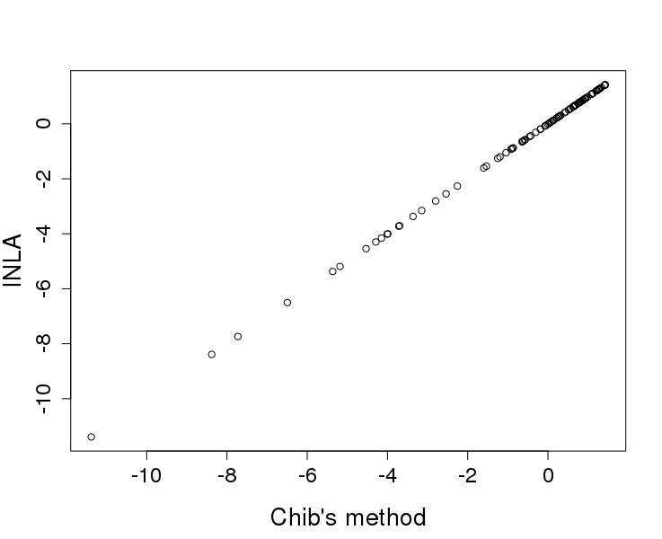
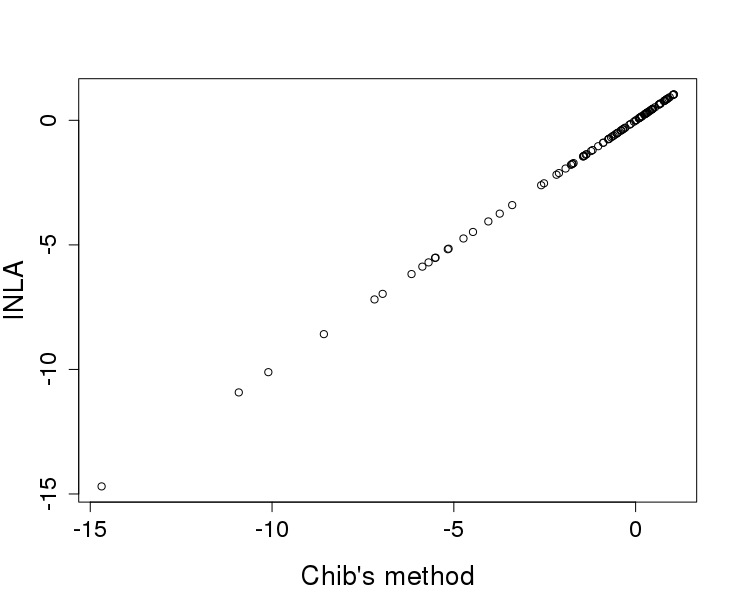
Figure 1: Chib’s-INLA plots of estimated marginal log-likelihoods obtained by Chib’s method ($x$-axis) and INLA ($y$-axis) for 100 different values of $\sigma_{\beta}^{-2}$. The left plot corresponds to model $\mathcal{M}_{1}$ while the right plot corresponds to model $\mathcal{M}_{2}$

Table 2 shows more details for a few chosen values of the standard deviation $\sigma_{\beta}$. The means of the 5 replications of Chib’s method all agree with INLA up to the second decimal.

$\mathcal{M}$	$\mu_{\beta}$	$\sigma_{\beta}$	INLA	Chib’s method
$\mathcal{M}_{1}$	0	1000	-73.2173	-73.2091	-73.2098	-73.2090	-73.2088	-73.2094
$\mathcal{M}_{1}$	0	10	-31.7814	-31.7727	-31.7732	-31.7732	-31.7725	-31.7733
$\mathcal{M}_{1}$	0	0.1	1.4288	1.4379	1.4380	1.4383	1.4378	1.4376
$\mathcal{M}_{2}$	0	1000	-96.6449	-96.6372	-96.6368	-96.6370	-96.6373	-96.6370
$\mathcal{M}_{2}$	0	10	-41.4064	-41.3989	-41.3987	-41.3991	-41.3995	-41.3996
$\mathcal{M}_{2}$	0	0.1	1.0536	1.0625	1.0629	1.0628	1.0626	1.0625

Table 2: Comparison of INLA and Chib’s method for marginal log likelihood.

Going a bit more into details, Figure 2 shows the performance of Chib’s method as a function of the number of iterations. The red circles in this graph represent 10 runs of Chib’s method for several choices of the number of iterations of the algorithm changing from 200 to 102400. The horizontal solid line shows the INLA estimate with default settings. In this case, we used a precision on the regression parameters equal to $\sigma^{-2}_{\beta}=0.2$, while in order to obtain some difference between Chib’s method and INLA we changed the mean to $\mu_{\beta}=1$. We only considered model $\mathcal{M}_{1}$ in this case. Although the differences are still small, this illustrates that INLA can be a bit off the true value. The reason for this deviance is due to the default choice of values for the tuning parameters in INLA. After tuning the step of numerical integration $\delta_{z}$ defining the grid as well as the convergence criterion of the differences of the log densities $\pi_{z}$ (Rue et al., 2009) one can make the difference between INLA and Chib’s method arbitrary small for this example. This can be clearly seen in Figure 2, where we depict the default INLA results (dark blue line) and the tuned INLA results (purple line).

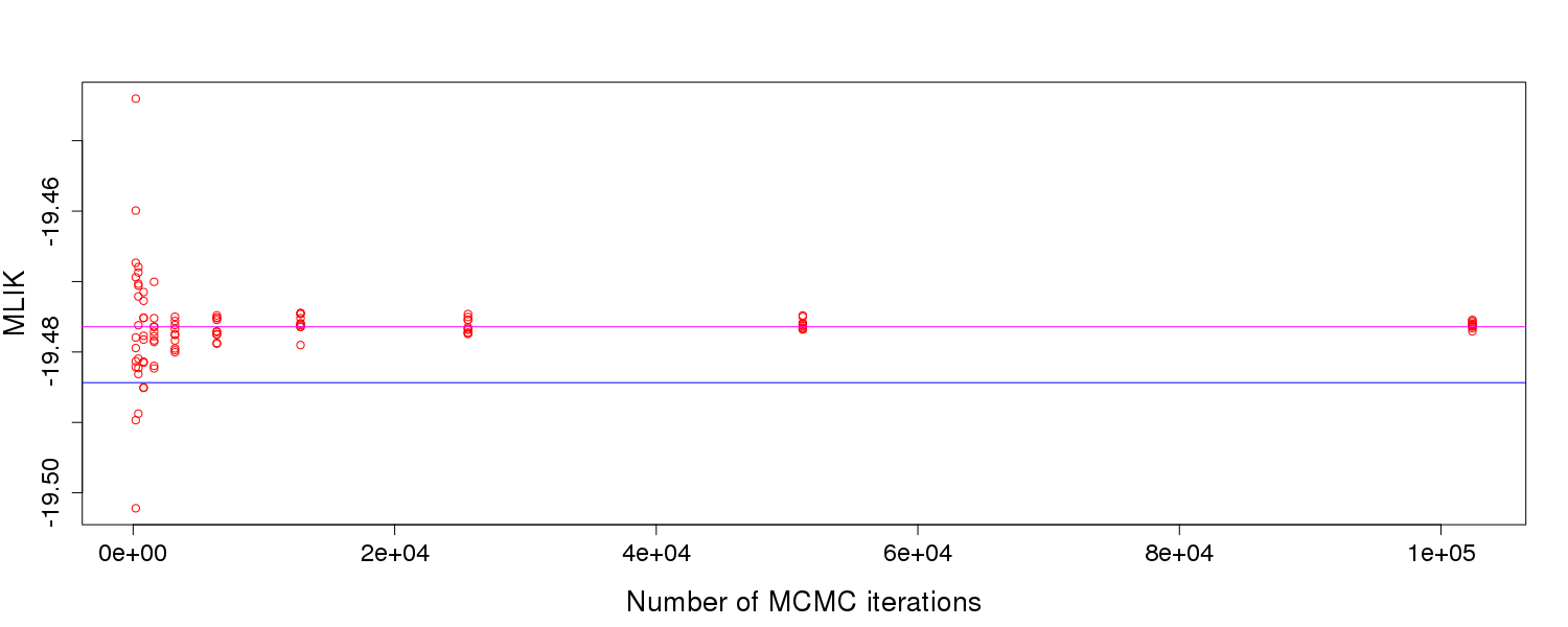
Figure 2: Variability of Chib’s method as a function of number of MCMC iterations for the simple linear Gaussian example. Horizontal lines correspond to INLA estimates based on default settings (dark blue) and adjusted settings (purple).

From Figure 2 one can also see that it might take quite a while for Chib’s method to converge, whilst INLA gives stable results for the fixed values of the tuning parameters. The total computational time for INLA corresponds to about 50 000 iterations with Chib’s method for this model. Whilst 819200 iterations of Chib’s method would require at least 15 times more time than INLA on the same machine .

The main conclusion that can be drawn from this example is that INLA approximations of marginal likelihoods can indeed be trusted for this model, giving yet another evidence in the support of INLA methodology in general.

4 INLA versus Chib’s method for logistic Bayesian regression with a probit link

In the third example we will continue comparing INLA with the Chib’s method (Chib, 1995) for approximating the marginal likelihood in logistic regression with a probit link model $\mathcal{M}$. The data set addressed is the simulated Bernoulli data introduced by Hubin and Storvik (2016). The model is given by

$$\begin{split}Y_{t}|p_{t},\mathcal{M}\stackrel{{\scriptstyle iid}}{{\sim}}&\text{ Bernoulli}(\Phi(\eta_{t}));\\ \eta_{t}|\mathcal{M}=&\beta_{0}+\sum_{i=1}^{p_{\mathcal{M}}}\beta_{i}x^{\mathcal{M}}_{ti};\\ \beta_{i}|\mathcal{M}\sim&N(\mu_{\beta},\sigma_{\beta}^{2}),\end{split}$$ (9)

where $t=1,...,2000$ and $i=0,...,p_{\mathcal{M}}$. We addressed two different sets of explanatory variables with different cardinalities of 11 for model $\mathcal{M}_{1}$ and 13 for model $\mathcal{M}_{2}$.

$\mathcal{M}$	$\mu_{\beta}$	$\sigma_{\beta}$	INLA	Chib’s method
$\mathcal{M}_{1}$	0	1000	-688.3192	-688.2463	-688.3260	-688.3117	-688.2613	-688.2990
$\mathcal{M}_{1}$	0	10	-633.0902	-633.1584	-633.0612	-633.0335	-633.1094	-633.0780
$\mathcal{M}_{1}$	0	0.1	-669.7590	-669.7646	-669.7666	-669.7610	-669.7465	-669.7528
$\mathcal{M}_{2}$	0	1000	-704.2266	-704.2154	-704.2138	-704.1463	-704.2526	-704.2303
$\mathcal{M}_{2}$	0	10	-639.8051	-639.7932	-639.8349	-639.8022	-639.7675	-639.8278
$\mathcal{M}_{2}$	0	0.1	-649.7803	-649.7360	-649.7604	-649.7893	-649.7532	-649.7806

Table 3: Comparison of INLA and Chib’s method for logistic Bayesian regression with a probit link

We used $\mu_{\beta}=0$ while the precisions for the regression parameters were varied between 0 and 10 in Figure 3 and chosen as $10^{-6},10^{-2}$ and $10^{2}$ in Table 3. Figure 3 shows that INLA and Chib’s method give reasonably similar results for both models.

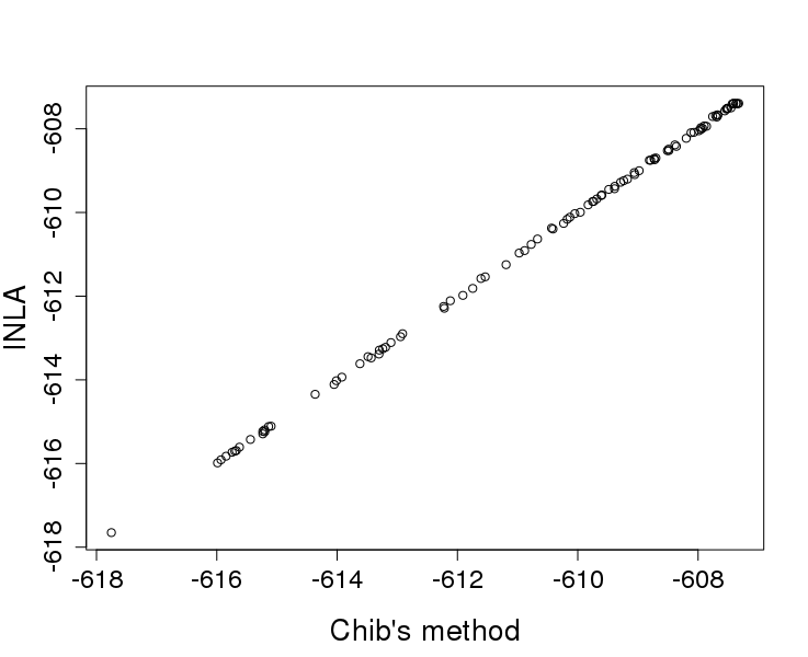
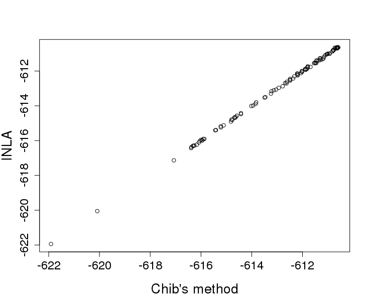
Figure 3: Comparisons of marginal likelihood estimates obtained by Chib’s method ($x$-axis) and INLA ($y$-axis) for 100 different values of the precision parameter $\sigma_{\beta}^{-2}$ under 2 models with different number of covariates.

The total time for running INLA within these examples is at most 2 seconds, corresponding to approximately 12000 MCMC iterations in Chib’s method. 100 000 MCMC iterations that were used to produce the obtained results in Table 3 required at least 25 seconds per replication on the same machine.

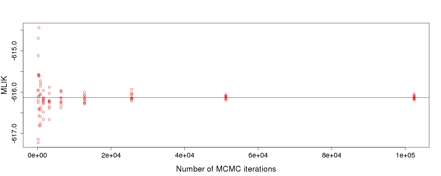
Figure 4: Variability of Chib’s method as a function of number of MCMC iterations for logistic Bayesian regression with a probit link. The horizontal line corresponds to the INLA estimate based on default settings.

5 INLA versus other methods for logistic Bayesian regression with a logit link

In the fourth example we will continue comparing marginal likelihoods obtained by INLA with such methods as Laplace approximations, Chib and Jeliazkov’s method, Laplace MAP approximations, harmonic mean method, power posteriors, annealed importance sampling and nested sampling. The model $\mathcal{M}$ is the Bayesian logistic regression model addressed by Friel and Wyse (2012), which is given by

$$\begin{split}Y_{t}|p_{t},\mathcal{M}\stackrel{{\scriptstyle iid}}{{\sim}}&\text{ Bernoulli}(\text{logit}^{-1}(\eta_{t}));\\ \eta_{t}|\mathcal{M}=&\beta_{0}+\sum_{i=1}^{p_{\mathcal{M}}}\beta_{i}x^{\mathcal{M}}_{ti};\\ \beta_{i}|\mathcal{M}\sim&N(\mu_{\beta},\sigma_{\beta}^{2}),\end{split}$$ (10)

where $t=1,...,532$ and $i=0,...,p_{\mathcal{M}}$. The data set addressed is the Pima Indians data, which consist of some diabetes records for $532$ Pima Indian women of different ages. For $\mathcal{M}_{1}$ we have addressed such predictors as the number of pregnancies, plasma glucose concentration, body mass index and diabetes pedigree function and for $\mathcal{M}_{2}$ we additionally consider the age covariate. All of the covariates for both of the models have been standardized before the analysis. Then the analysis was performed for $\sigma_{\beta}^{2}=100$ and $\sigma_{\beta}^{2}=1$ correspondingly. The prior value of $\mu_{\beta}$ for both of the cases was chosen to be equal to 1. Table 4 contains the results obtained by all of the methods. Notice that all of the calculations apart from the INLA based ones are reported in Friel and Wyse (2012). Friel and Wyse (2012) claim that the relevant measures were taken to make the implementation of each method as fair as possible. In their runs each Monte Carlo method used the equivalent of 200 000 samples. In particular, the power posteriors used 20 000 samples at each of the 10 steps. The annealed importance sampling a cooling scheme with 100 temperatures and 2 000 samples generated per temperature. Nested sampling was allowed to use 2 000 samples and was terminated when the contribution to the current value of marginal likelihood was smaller than $10^{-8}$ times the current value. Notice that the default tuning parameters were applied for the INLA calculations. Except for the Harmonic mean, all methods gave comparable results. The INLA method only needed a computational time comparable to Laplace approximations, which is much faster than the competing approaches (Friel and Wyse, 2012). Reasonably good performance of the ordinary Laplace approximation in this case can be explained by having no latent variables in the model.

Method	$\mathcal{M}_{1}$	$\mathcal{M}_{2}$	$\mathcal{M}_{1}$	$\mathcal{M}_{2}$
INLA	-257.25	-259.89	-247.32	-247.59
Laplace approximation	-257.26	-259.89	-247.33	-247.59
Chib and Jeliazkov’s method	-257.23	-259.84	-247.31	-247.58
Laplace approximation MAP	-257.28	-259.90	-247.33	-247.62
Harmonic mean estimator	-279.47	-284.78	-259.84	-260.55
Power posteriors	-257.98	-260.59	-247.57	-247.84
Annealed importance sampling	-257.87	-260.43	-247.30	-247.59
Nested sampling	-258.82	-261.38	-246.82	-246.97
$\sigma_{\beta}^{2}$ value	100	100	1	1

Table 4: Comparison of INLA and other method for a logistic Bayesian regression with a logit link.

6 INLA versus Chib and Jeliazkov’s method for computation of marginal likelihoods in a Poisson with a mixed effect model

As models become more sophisticated we have less methodologies that can be used for approximating the marginal likelihood. In the context of generalized linear mixed models two alternatives will be considered, the INLA approach (Rue et al., 2009) and the Chib and Jeliazkov’s approach (Chib and Jeliazkov, 2001).

This model is concerned with seizure counts $Y_{jt}$ for 59 epileptics measured first over an 8-week baseline period $t=0$ and then over 4 subsequent 2-week periods $t=1,...,4$. After the baseline period each patient is randomly assigned to either receive a specific drug or a placebo. Following previous analyses of these data, we removed observation 49, considered to be an outlier because of the unusual seizure counts. We assume the data to be Poisson distributed and model both fixed and random effects of based on some covariates. The model $\mathcal{M}$, originally defined in Diggle et al. (1994), is given by

$$\begin{split}Y_{jt}|\lambda_{jt},\mathcal{M}\sim&\text{ Poisson}(\exp(\eta_{jt}));\\ \eta_{jt}|\mathcal{M}=&\log(\tau_{jt})+\beta_{0}+\beta_{1}x_{jt1}+\beta_{1}x_{jt2}+\beta_{3}x_{jt1}x_{jt2}+b_{j0}+b_{j1}x_{jt1};\\ \beta_{i}|\mathcal{M}\sim&N(0,100),\quad\quad i=0,...,3;\\ \mathbb{b_{j}}|\mathbf{D},\mathcal{M}\sim&N_{2}(0,\mathbf{D});\\ \mathbf{D}^{-1}|\mathcal{M}\sim&\text{ Wishart}_{2}(4,I_{2}),\end{split}$$ (11)

for $j=1,...,58,t=1,...,4$. Here $x_{jt1}\in\{0,1\}$ is an indicator variable of period (0 if baseline and 1 otherwise), $x_{jt2}\in\{0,1\}$ is an indicator for treatment status, $\tau_{it}$ is the offset that is equal to 8 in the baseline period and 2 otherwise, and $\mathbb{b_{j}}$ are latent random effects. In Chib and Jeliazkov (2001) an estimate of the marginal log-likelihood was reported to be -915.49, while also an alternative estimate equal to -915.23 based on a kernel density approach by Chib et al. (1998) was given. INLA gave a value of -915.61 in this case, again demonstrating its accuracy. The computational time for the INLA computation was in this case on average 1.85 seconds.

7 Conclusions

The marginal likelihood is a fundamental quantity in the Bayesian statistics, which is extensively adopted for Bayesian model selection and averaging in various settings. In this study we have compared the INLA methodology to some other approaches for approximate calculation of the marginal likelihood. In all of the addressed examples disregarding complexity of the latter INLA gave reliable estimates. In all cases, default settings of the INLA procedure gave reasonable accurate results. If extremely high accuracy is needed we recommend that before performing Bayesian model selection and averaging in a particular model space $\Omega_{\mathcal{M}}$ based on marginal likelihoods produced by INLA, the produced estimates should be carefully studied and the tuning parameters adjusted, if required. Experimenting with different settings will also give an indication on whether more accuracy is needed.

SUPPLEMENTARY MATERIAL

Data and code: Data (simulated and real) and R scripts for calculating marginal likelihoods under various scenarios are available online at https://goo.gl/0Wsqgp.

ACKNOWLEDGMENTS

We would like to thank CELS project at the University of Oslo for giving us the opportunity, inspiration and motivation to write this article.

References

- Chib (1995) S. Chib. Marginal likelihood from the Gibbs output. Journal of the American Statistical Association, 90(432):1313–1321, 1995.
- Chib and Jeliazkov (2001) S. Chib and I. Jeliazkov. Marginal likelihood from the Metropolis–Hastings output. Journal of the American Statistical Association, 96(453):270–281, 2001.
- Chib et al. (1998) S. Chib, E. Greenberg, and R. Winkelmann. Posterior simulation and Bayes factors in panel count data models. Journal of Econometrics, 86(1):33 – 54, 1998.
- Diggle et al. (1994) P. Diggle, K. Liang, and S. Zeger. Analysis of longitudinal data oxford, 1994.
- Friel and Wyse (2012) N. Friel and J. Wyse. Estimating the evidence – a review. Statistica Neerlandica, 66(3):288–308, 2012. ISSN 1467-9574.
- Hubin and Storvik (2016) A. Hubin and G. Storvik. Efficient mode jumping MCMC for Bayesian variable selection in GLMM. arXiv preprint arXiv:1604.06398, 2016.
- Jordan et al. (1999) M. I. Jordan, Z. Ghahramani, T. S. Jaakkola, and L. K. Saul. An introduction to variational methods for graphical models. Machine learning, 37(2):183–233, 1999.
- Kass and Raftery (1995) R. E. Kass and A. E. Raftery. Bayes factors. Journal of the american statistical association, 90(430):773–795, 1995.
- Marin et al. (2012) J.-M. Marin, P. Pudlo, C. P. Robert, and R. J. Ryder. Approximate Bayesian computational methods. Statistics and Computing, 22(6):1167–1180, 2012.
- McGrory and Titterington (2007) C. A. McGrory and D. Titterington. Variational approximations in Bayesian model selection for finite mixture distributions. Computational Statistics & Data Analysis, 51(11):5352–5367, 2007.
- Neal (2008) R. Neal. The Harmonic Mean of the Likelihood: Worst Monte Carlo Method Ever, 2008.
- Newton and Raftery (1994) M. A. Newton and A. E. Raftery. Approximate Bayesian inference with the weighted likelihood bootstrap. Journal of the Royal Statistical Society. Series B (Methodological), pages 3–48, 1994.
- Raftery et al. (2006) A. E. Raftery, M. A. Newton, J. M. Satagopan, and P. N. Krivitsky. Estimating the integrated likelihood via posterior simulation using the harmonic mean identity. 2006.
- Rue et al. (2009) H. Rue, S. Martino, and N. Chopin. Approximate Bayesian inference for latent Gaussian models by using integrated nested Laplace approximations. Journal of the Royal Statistical Sosciety, 71(2):319–392, 2009.
- Tierney and Kadane (1986) L. Tierney and J. B. Kadane. Accurate approximations for posterior moments and marginal densities. Journal of the american statistical association, 81(393):82–86, 1986.
- Vandaele (2007) W. Vandaele. Participation in illegitimate activities: Ehrlich revisited. Deterrence and Incapacitation, pages 270–335, 2007.