Liquidity induced asset bubbles via flows of ELMMs

Abstract

We consider a constructive model for asset price bubbles, where the market price $W$ is endogenously determined by the trading activity on the market and the fundamental price $W^{F}$ is exogenously given, as in [28]. To justify $W^{F}$ from a fundamental point of view, we embed this constructive approach in the martingale theory of bubbles, see [26] and [10], by showing the existence of a flow of equivalent martingale measures for $W$, under which $W^{F}$ equals the expectation of the discounted future cash flow.
As an application, we study bubble formation and evolution in a financial network.

Keywords: Bubbles, Equivalent martingale measures, Financial networks, Liquidity based model

1 Introduction

The formation of asset price bubbles has been thoroughly investigated from an economical point of view in many contributions, see Tirole [45], Allen and Gale [3], Choi and Douady [13], [14], Harrison and Kreps [22], Kaizoji [29], Earl et al. [18], DeLong, Shleifer, Summers and Waldmann [17], Scheinkman and Xiong [43], [44], Xiong [49], Abreu and Brunnermeier [1], Föllmer, Horst, and Kirman [20], Miller [35], Zhuk [50].
Different causes have been indicated as triggering factors for bubble birth, such as heterogenous beliefs between interacting agents (as in [20], [22], [43], [44], [49], [50]), a breakdown of the dynamic stability of the financial system ([13], [14]), the diffusion of new investment decision rules from a few expert investors to larger population of amateurs (see [18]), the tendency of traders to choose the same behavior as the other traders’ behavior as thoroughly as possible (see [29]), the presence of short-selling constraints (see [35]).
From the mathematical point of view, one of the main approaches is given by the martingale theory of bubbles as introduced by Cox and Hobson [16] and Loewenstein and Willard [30] and mainly developed by Jarrow, Protter et al. [23], [24], [25], [26], [27]. See Protter [41] for an overview. In this setting a $Q$-bubble is defined as the difference between the market price of a given financial asset and its fundamental value, given by the expectation of the future cash flows under an equivalent local martingale measure $Q$.
Defined in this way, the bubble is a non-negative local martingale under $Q$, and it is strictly positive if and only if the market wealth $W$ is a strict $Q$-local martingale (for a complete analysis, see for example [10], [16], [25], [26], [30], [41]).
In a complete market (see [25]), where only one equivalent local martingale measure (ELMM) exists, only two possibilities are given: either no bubble appears at all, or a bubble is already present at the beginning. This is a strong modeling withdraw, therefore in [26] and [10] incomplete markets have been taken into consideration: the birth and the evolution of a bubble are then determined by a flow of different ELMMs that gives rise to a corresponding shifting perception of the fundamental value of the asset. In [26] the underlying pricing measures may change only at certain stopping times, in [10] a continuous flow in the space of martingale measures is considered.
On the other hand, an alternative model is given by Jarrow, Protter and Roch in [28], where the fundamental value is exogenously given, whereas the market value is endogenously determined by the trading activity of investors, and studied through the analysis of the liquidity supply curve. For another constructive model, see also [9].
In this setting a bubble is still defined as the difference between the market value $W$ and the fundamental value $W^{F}$, however it does not always coincide with the $Q$-bubble under a given equivalent martingale measure $Q$.
A natural question is then if it is possible to embed a constructive model, where the fundamental price is exogenous and the market price endogenous, in the martingale theory of bubbles, by determining a suitable flow of ELMMs for $W$ under which $W^{F}$ is justified from a fundamental point of view.
More precisely, given a liquidation time $T$ for the financial asset, we look for a flow $(Q^{t})_{t\in[0,T)}$ of ELMMs for the market wealth $W$ such that the fundamental value of the asset is given as the expectation of the future cash flow as in equation (3.1). Note however that we do not obtain that $W^{F}$ is also a (local) martingale under each measure of the flow, as thoroughly discussed in Remark 3.1.
Our main result is then that we can explicitly determine the form of such a flow of ELMMS in a liquidity driven model under very general assumptions, see Theorem 3.16. This require a consistent technical effort, mostly devoted to guarantee the martingale property of the chosen flows of (eventual) probability densities. In this way we are able to directly connect the impact of the underlying macro-economic factors to the shift of the resulting pricing measure, which may change over time.
As an application of our method, we consider the evolution of a bubble in a financial network and compute the generating flow of ELMMs. However, this example is also of independent interest, as it studies how the interaction of market participants in a financial network can affect asset price formation and the consequent birth of a bubble. Different studies show how contagion between investors and herding behavior may play an essential role when a bubble grows up: euphoria and exuberance can propagate among market participants, due to exchanges of ideas (see Lux [31]) or to the fact that investors may be attracted by the short period earnings of acquaintances investing in the bubbly asset, as observed by Bayer et al. in [8], where analyzing data from the housing bubble in L. A. in the 2000s the authors notice a strong contagion between neighbors.
Several contributions in the last years has been focusing on how some properties of the network, like mean degree or degree heterogeneity, can influence the contagion of failures and losses between banks during a financial crisis (see for example Acemoglu et al. [2], Allen and Gale [4], Amini et al. [5], Cont et al. [15], Gai and Kapadia [21], Newman et al. [37], Watts [46], Watts and Strogatz [47]). Some investigation has been proposed about how bubbles are generated at the microeconomic level by the interaction of market participants (see among others Lux [31], Scheinkman [43], Scheinkman and Xiong [44], Tirole [45], Zhuk [50]). However, only a few studies have been devoted to understand how the structure of a given financial network can influence the spread of contagion between investors that generates a bubble. In [31], for example, the author models the bubble as caused by a self-organizing process of infection between traders, expressed by a system of PDEs, leading to equilibrium prices that deviate from the fundamental value. However they consider a world in which everybody is connected with everybody, so that the network structure does not enter into play.
In our special case we focus on a model for the aggregate trading volume of $X$ in dependence by some characteristics of the underlying networks of investors, such as the degree distribution. In particular we use some modeling approach deriving from the literature on infectious processes in a population by following the so called SIS model (see Pastor-Satorras and Vespignani [38] and [39]). We provide numerical simulations to investigate how different networks generate different contagion mechanisms and then to bubbles with different evolutions. In particular, it turns out that in more heterogenous networks (i.e. networks with a more right skewed degree distribution) contagion spread faster at the beginning so that the bubble builds up faster and bursts sooner: the nodes with high degree, which in average get infected faster, contribute with an higher weight in the more right skewed distributions.
The paper is therefore organized as follows: in Section 2 we describe the setting of the liquidity model, define the fundamental value of the asset and specify how the trading activity of investors influences the market price of the asset. In Section 3 we determine a possible flow $(Q^{t})_{t\in[0,T)}$ of ELMMs satisfying (3.1) and show that the density process $(Z_{t,s})_{s\in[0,T)}$ with $Z_{t,s}=\frac{dQ^{t}}{dP}|_{\mathcal{F}_{s}}$ is a true martingale wrt $s$. In Section 4 we give an example showing how contagion between investors can develop the bubble in a network and compute the generating flow of ELMMs.

2 The Setting

Let $(\Omega,\mathcal{F},P)$ be a probability space and $T>0$ a random time on it, representing the maturity or liquidation time of the underlying risky asset as in the setting of [26]. We assume that $(\Omega,\mathcal{F},P)$ is endowed with a filtration $\mathbb{F}=(\mathcal{F}_{t})_{t\in[0,T]}$ satisfying the usual assumptions of completeness and right continuity.
On $(\Omega,\mathcal{F},\mathbb{F},P)$ we have ($B^{1},B^{2},B^{3},B^{4},N$), where $B^{i}=(B^{i}_{t})_{t\in[0,T]}$, $i=1,2,3,4$ are standard $\mathbb{F}$-Brownian motions and $N_{t}=\mathbb{1}_{\{\tau\leq t\}}$ is a jump process with $\tau$ totally inaccessible stopping time with intensity process $\pi=(\pi_{t})_{t\in[0,T]}$. We assume that ($B^{1},B^{2},B^{3},B^{4},N$) are independent processes.
Following [28] we consider a financial asset whose fundamental wealth $W^{F}=(W_{t}^{F})_{t\in[0,T]}$ (associated to the cumulative dividend process $(D_{t})_{t\in[0,T]}$ and to the liquidation value $F$ of the asset at time $T$) is given by

$$dW_{t}^{F}=W_{t}^{F}(adt+bdB_{t}^{1}),\quad 0\leq t\leq T,$$ (2.1)

with $W_{0}^{F}>0$, $a>0$ and $b>0$.
We interpret $\tau$ as the time of birth of a bubble for this financial asset. The bubble follows the dynamics

$$d\beta_{t}=M_{t}\Lambda_{t}(-k\beta_{t}dt+2dX_{t}+2xW_{t}^{F}dN_{t}),\quad 0\leq t<T,$$ (2.2)

where $X$ is the aggregate trading volume (buy market orders minus sell market orders), $x$ is the aggregate trading volume at $\tau$ and $M=(M_{t})_{t\in[0,T]}$, $\Lambda=(\Lambda_{t})_{t\in[0,T]}$ are respectively a measure of illiquidity and the so called resiliency (for an economical motivation of this setting we refer to [28]). We put $\beta_{\tau}=2x\Lambda_{\tau}M_{\tau}W_{\tau}^{F}$ for a given $x>0$.
We consider that $X$ satisfies the following dynamics

$$X_{t}=0, \text{for }0\leq t<\tau,$$

$$dX_{t}=\mu_{t}dt+\sigma_{t}dB_{t}^{2}, \text{ for }\tau\leq t<T,$$ (2.3)

where $\mu=(\mu_{t})_{t\in[0,T]}$ and $\sigma=(\sigma_{t})_{t\in[0,T]}$ are progressively measurable processes that a priori can also depend on $X$ itself or on the bubble $\beta$.
In [28] the aggregate trading volume is modeled as in (2.3) with $\mu\equiv 0$ and $\sigma_{t}=\alpha\beta_{t}$. Here we introduce the drift $\mu$ in order to see the influence of the network on the size of the bubble, as we specify in Section 4.
Here the fundamental wealth process $W^{F}$ is exogenously given, while the market wealth process $W=(W_{t})_{t\in[0,T]}$ is endogenously determined as

$$W_{t}=W_{t}^{F}+\beta_{t},\quad 0\leq t<T.$$

At liquidation time $T$ we have $W_{T}=W_{T}^{F}$: the asset is liquidated at time $T$ at the estimated firm’s value, i.e. at the fundamental value. In particular we require in the sequel that there exists an equivalent local martingale measure for $W$ only on the open interval $[0,T)$, since around time $T$ the liquidation procedure is not subjected to market equilibrium mechanisms.

Assumption 2.1.

1. $\int_{\tau}^{T}\mu_{s}^{2}ds<\infty$ a.s.

2. $\int_{\tau}^{T}\sigma_{s}^{2}ds<\infty$ a.s. and $\int_{\tau}^{T}\frac{1}{\sigma_{s}^{4}}ds<\infty$ a.s.

3. $\mu$ and $\sigma$ are such that there exists a unique solution of (2.3) (see for example Theorem 7 in Chapter V.3 in [40]);

4. $M=(M_{t})_{t\in[0,T]}$ is an adapted process that satisfies the dynamics

   $$dM_{t}=\tilde{\mu}(M_{t})dt+\tilde{\sigma}(M_{t})dB^{3}_{t},\quad 0\leq t\leq T,$$

   where $\tilde{\mu}$ and $\tilde{\sigma}$ are such that there exists a unique solution of (iv) according to Theorem 7 in Chapter V.3 in [40]. Moreover $\int_{a}^{b}\tilde{\sigma}^{-4}(x)dx<\infty$ for every $a,b$ such that $0<a<b<\infty$.

5. $\Lambda=(\Lambda_{t})_{t\in[0,T]}$ satisfies the dynamics

   $$d\Lambda_{t}=\mu^{\prime}(\Lambda_{t})dt+\sigma^{\prime}(\Lambda_{t})dB^{4}_{t},\quad 0\leq t\leq T,$$

   $\Lambda_{0}\in(\lambda,1)$, with $\mu^{\prime}$, $\sigma^{\prime}$ that satisfy conditions Theorem 7 in Chapter V.3 in [40]. Furthermore $\mu^{\prime}(\lambda)>0$, $\mu^{\prime}(1)<0$, $\sigma^{\prime}(1)=0$, $\sigma^{\prime}(\lambda)=0$ a.s., so that we obtain $\lambda\leq\Lambda_{t}\leq 1$, a.s. for all $t\in[0,T]$.

6. $\pi=(\pi_{t})_{t\in[0,T]}$ is bounded, i.e. $|\pi_{t}|\leq\Pi<\infty$ a.s for all $t\in[0,T]$.

7. $T$ is a bounded a.s. (possibly by a very large constant) $\mathbb{F}$-stopping time independent of $(B^{1},B^{2},N)$ such that $\tau<T$ a.s.

Notice that we assume $\tau<T$ and $T$ bounded a.s. for the sake of simplicity. The following results still hold without these conditions by imposing some integrability conditions on $T$. For example, it would be sufficient $T<\infty$ a.s., $\mathbb{E}_{P}[e^{T}|\mathcal{F}_{t}]<\infty$ and $\mathbb{E}_{P}[T-\tau|\mathcal{F}_{t}]>0$ a.s. for $t\in[0,T]$.

Remark 2.2.

Here we exclude that $\sigma$ can depend on $\beta$. However the following results also hold for the case $\sigma_{t}=\alpha\beta_{t}$, $t\in[\tau,T]$, $\alpha\in\mathbb{R}$, considered in [28] to model the evolution of the bubble given by illiquidity effects. We refer to [32] for more details in this case.

Proposition 2.3.

From the hypothesis on $M$ it follows that $\int_{0}^{T}M_{s}^{\alpha}ds<\infty$ a.s. for all $\alpha\in\mathbb{R}$.

Proof. Following the same argument as in [34], we have that

$$\int_{0}^{T}M_{s}^{\alpha}ds= \int_{0}^{T}\frac{M_{s}^{\alpha}}{\tilde{\sigma}^{2}(M_{s})}d[M,M]_{s}=\int_{0}^{\infty}\frac{x^{\alpha}}{\tilde{\sigma}^{2}(x)}L_{T}^{x}dx,$$ (2.4)

where $L_{T}^{x}$ is the local time at $T$ and the last equality follows by occupation time formula (see for example Corollary 1 in Chapter IV of [40]).
Then the integral is finite since, by the fact that $0<M_{s}<\infty$ a.s. for each $s\in[0,T]$, we have that the occupation time $L_{T}^{a}$ has compact support in $(0,\infty)$. $\quad\Box$.

From Remark 2.2 we have that $\beta$ satisfies the SDE

$$d\beta_{t}=2\Lambda_{t}M_{t}\left[(-k\beta_{t}+\mu_{t})dt+\sigma_{t}dB_{t}^{2}+xW_{t}^{F}dN_{t}\right],\quad\tau\leq t<T.$$

The bubble takes therefore the following explicit expression:

$$\beta_{t}= \beta_{\tau}e^{-k\int_{\tau}^{t}\Lambda_{s}M_{s}ds}+\int_{\tau}^{t}\mu_{s}\Lambda_{s}M_{s}e^{-k\int_{s}^{t}\Lambda_{u}M_{u}du}ds+$$

$$+\int_{\tau}^{t}\sigma_{s}\Lambda_{s}M_{s}e^{-k\int_{s}^{t}\Lambda_{u}M_{u}du}dB_{s}^{2},\quad\tau\leq t<T.$$ (2.5)

3 Flow of equivalent local martingale measures

Let $\mathcal{M}_{loc}(W)$ be the space of equivalent local martingale measures for $W$. Given $Q\in\mathcal{M}_{loc}(W)$, a $Q$-bubble $\beta^{Q}$ is defined as

$$\beta_{t}^{Q}=W_{t}-\mathbb{E}_{Q}[W_{T}|\mathcal{F}_{t}]$$

in the approach of [25] and [26]. In particular we have that the bubble introduced in (2.2) coincides with a $Q$-bubble if and only if

$$W_{t}^{F}=\mathbb{E}_{Q}[W_{T}|\mathcal{F}_{t}],\quad t\in[0,T]$$

for some $Q\in\mathcal{M}_{loc}(W)$.
This is of course not possible in our setting. However we can find a flow $(Q^{t})_{t\in[0,T]}\subseteq\mathcal{M}_{loc}(W)$ such that

$$W_{t}^{F}=\mathbb{E}_{Q^{t}}[W_{T}|\mathcal{F}_{t}]=\mathbb{E}_{Q^{t}}[W_{T}^{F}|\mathcal{F}_{t}].$$ (3.1)

In this way the bubble described in (2.2) is the result of the shift in the pricing measure induced by the change in the macro-economic and financial conditions in the market.

Remark 3.1.

Note that (3.1) does not imply that $W^{F}$ is a martingale under $Q^{t}$. Eq. (3.1) holds $t$-wise and in general it is not true that

$$W_{s}^{F}=\mathbb{E}_{Q^{t}}[W_{T}|\mathcal{F}_{s}]$$

for $s\neq t$. Furthermore $Q^{t}$ is an equivalent local martingale measure for $W$ only on $[0,T)$.

We now explicitly compute a flow $(Q^{t})_{t\in[0,T)}\in\mathcal{M}_{loc}(W)$ justifying the existence of the bubble in (2.2) from a fundamental point of view.
Let $Q\in\mathcal{M}_{loc}(W)$. Then the density process $Z=(Z_{t})_{t\in[0,T)}$ of $Q$ with respect to $P$ is given by

$$Z_{t}=\frac{dQ}{dP}|_{\mathcal{F}_{t}}=\mathcal{E}\left(\int_{0}^{\cdotp}\alpha_{s}^{1}dB_{s}^{1}+\int_{0}^{\cdot}\alpha_{s}^{2}dB_{s}^{2}+\int_{0}^{\cdot}\alpha_{s}^{3}d\tilde{N}_{s}+\int_{0}^{\cdot}\alpha_{s}^{4}dB_{s}^{3}+\int_{0}^{\cdot}\alpha_{s}^{5}dB_{s}^{4}+L_{t}\right)_{t},$$

$0\leq t<T$, where $\tilde{N}_{t}=N_{t}-\int_{0}^{t\wedge\tau}n_{s}ds$, $t\in[0,T)$, $L$ is a martingale strongly orthogonal to ($B^{1},B^{2},B^{3},B^{4},N$) and the processes $\alpha^{i}$, $i=1,\dots,5$ are such that for $0\leq s<T$ the following equality holds:

$$W_{s}^{F}(a+b\alpha^{1}_{s})+2\Lambda_{s}M_{s}\left(\mu_{s}+\sigma_{s}\alpha_{s}^{2}-k\beta_{s}\right)\mathbb{1}_{\{s\geq\tau\}}+2\pi_{s}xW_{s}^{F}\Lambda_{s}M_{s}(\alpha_{s}^{3}+1)\mathbb{1}_{\{s<\tau\}}=0.$$ (3.2)

Since (3.2) does not involve $\alpha^{4}$, $\alpha^{5}$ or $L$, we put $\alpha^{4}\equiv\alpha^{5}\equiv L\equiv 0$.
We can split (3.2) as

$$b\alpha^{1}_{s}=-a-2\pi_{s}x\Lambda_{s}M_{s}(\alpha_{s}^{3}+1)\quad\text{for }s<\tau$$ (3.3)

and

$$b\alpha^{1}_{s}=-a+\frac{2\Lambda_{s}M_{s}}{W_{s}^{F}}\left(k\beta_{s}-\mu_{s}-\sigma_{s}\alpha_{s}^{2}\right)\quad\text{for }s\geq\tau.$$ (3.4)

We look for a flow of the form

$$Z_{t,s}=\frac{dQ^{t}}{dP}|_{\mathcal{F}_{s}}=\mathcal{E}\left(\int_{0}^{\cdot}\alpha_{u}^{t,1}dB_{u}^{1}+\int_{0}^{\cdot}\alpha_{u}^{t,2}dB_{u}^{2}+\int_{0}^{\cdot}\alpha_{u}^{t,3}d\tilde{N}_{u}\right)_{s},\quad s\in[0,T),$$ (3.5)

since (3.2) does not involve conditions on $\alpha^{t,4}$, $\alpha^{t,5}$ and $\alpha^{t,6}$. In particular, we note that the laws of $M$, $\Lambda$ and $T$ are invariant under this change of measure.
If $\alpha^{t,1}$, $\alpha^{t,2}$ and $\alpha^{t,3}$ satisfy (3.3) and (3.4), the fundamental process under $Q^{t}$ is given by

$$\frac{dW_{s}^{F}}{W_{s}^{F}}=\tilde{\mu}_{s}^{t}ds+bd\tilde{B}_{s}^{t},\quad 0\leq s\leq T,$$ (3.6)

where $\tilde{B}^{t}$ denote the $Q^{t}$-standard Brownian motion given by

$$\tilde{B^{t}_{s}}=B_{s}^{1}-\int_{0}^{s}\alpha_{u}^{t,1}du,\quad 0\leq s\leq T,$$

and

$$\tilde{\mu}_{s}^{t}=\begin{cases}-2\pi_{s}x\Lambda_{s}M_{s}(\alpha_{s}^{t,3}+1)\quad&\text{for }s<\tau,\\ \frac{2\Lambda_{s}M_{s}}{W_{s}^{F}}\left(k\beta_{s}-\mu_{s}-\sigma_{s}\alpha_{s}^{t,2}\right)\quad&\text{for }s\geq\tau.\end{cases}$$ (3.7)

If the condition

$$\mathbb{E}_{Q^{t}}\left[\int_{t}^{T}(W_{s}^{F})^{2}ds\right]<\infty$$ (3.8)

is satisfied, we have that (3.1) is equivalent to

$$\mathbb{E}_{Q^{t}}\left[\int_{t}^{T}W_{s}^{F}\tilde{\mu}_{s}^{t}ds\Big{|}\mathcal{F}_{t}\right]=0,$$

that is

$$0=\mathbb{E}_{Q^{t}} \left[\int_{t}^{\tau}W_{s}^{F}\pi_{s}x\Lambda_{s}M_{s}(\alpha_{s}^{t,3}+1)ds+\int_{\tau}^{T}\Lambda_{s}M_{s}\left(k\beta_{s}-\mu_{s}-\sigma_{s}\alpha_{s}^{t,2}\right)ds\Big{|}\mathcal{F}_{t}\right]$$ (3.9)

for $t<\tau$ and

$$\mathbb{E}_{Q^{t}}\left[\int_{t}^{T}\Lambda_{s}M_{s}\left(k\beta_{s}-\mu_{s}-\sigma_{s}\alpha_{s}^{t,2}\right)ds\Big{|}\mathcal{F}_{t}\right]=0$$ (3.10)

for $t\geq\tau$.
To show the existence of the flow $(Q^{t})_{t\in[0,T)}\subseteq\mathcal{M}_{loc}(W)$, we choose $\alpha^{t,2}$ and $\alpha^{t,3}$ so that the integrals inside the conditional expectation in (3.9) and (3.10) are zero almost surely. We show later on that a posteriori this choice ensures as well that (3.8) holds.
For $t\geq\tau$, let

$$\alpha_{s}^{t,2}=\frac{1}{\Lambda_{s}M_{s}\sigma_{s}}\left(s-\frac{\mathbb{E}[T|\mathcal{F}_{t}]+t}{2}+\frac{\mathbb{E}^{2}[T|\mathcal{F}_{t}]-\mathbb{E}[T^{2}|\mathcal{F}_{t}]}{2(\mathbb{E}[T|\mathcal{F}_{t}]-t)}\right)+\frac{k\beta_{s}}{\sigma_{s}}-\frac{\mu_{s}}{\sigma_{s}},\quad t\leq s<T.$$

Notice that such $\alpha_{s}^{t,2}$ is well defined since from Assumption 2.1 it holds $\Lambda_{s}>0$, $M_{s}>0$, $\sigma_{s}>0$ a.s. for every $s\in[0,T]$.
With this choice we have on $\{T>t\}$ that

$$\mathbb{E}_{\mathbb{Q}^{t}}\left[\int_{t}^{T}\Lambda_{s}M_{s}\left(k\beta_{s}-\mu_{s}-\sigma_{s}\alpha_{s}^{t,2}\right)ds\Big{|}\mathcal{F}_{t}\right]$$

$$= \mathbb{E}_{\mathbb{Q}^{t}}\left[\int_{t}^{T}\left(s-\frac{\mathbb{E}[T|\mathcal{F}_{t}]+t}{2}+\frac{\mathbb{E}^{2}[T|\mathcal{F}_{t}]-\mathbb{E}[T^{2}|\mathcal{F}_{t}]}{2(\mathbb{E}[T|\mathcal{F}_{t}]-t)}\right)ds\Big{|}\mathcal{F}_{t}\right]$$

$$= \mathbb{E}_{\mathbb{Q}^{t}}\left[\left(\frac{T^{2}-t^{2}}{2}-(T-t)\frac{\mathbb{E}[T|\mathcal{F}_{t}]+t}{2}+(T-t)\frac{\mathbb{E}^{2}[T|\mathcal{F}_{t}]-\mathbb{E}[T^{2}|\mathcal{F}_{t}]}{2(\mathbb{E}[T|\mathcal{F}_{t}]-t)}\right)\Big{|}\mathcal{F}_{t}\right]$$

$$= \frac{\mathbb{E}[T^{2}|\mathcal{F}_{t}]-t^{2}}{2}-\frac{(\mathbb{E}[T|\mathcal{F}_{t}]-t)(\mathbb{E}[T|\mathcal{F}_{t}]+t)}{2}+\frac{\mathbb{E}^{2}[T|\mathcal{F}_{t}]-\mathbb{E}[T^{2}|\mathcal{F}_{t}]}{2}=0,$$ (3.11)

since by Assumption 2.1 the law of $T$ does not change under $Q^{t}$.
For $t<\tau$ define

$$C_{t,\tau}:=\int_{t}^{\tau}W_{s}^{F}\pi_{s}x\Lambda_{s}M_{s}(\alpha_{s}^{t,3}+1)ds$$

and choose $\alpha^{t,2}_{s}$ to be such that

$$\mathbb{E}_{Q^{t}}\left[\int_{\tau}^{T}\Lambda_{s}M_{s}\left(k\beta_{s}-\mu_{s}-\sigma_{s}\alpha_{s}^{t,2}\right)ds\Big{|}\mathcal{F}_{t}\right]=-\mathbb{E}_{Q^{t}}\left[C_{t,\tau}|\mathcal{F}_{t}\right],$$

i.e.

$$\alpha_{s}^{t,2}= \frac{1}{\Lambda_{s}M_{s}\sigma_{s}}\left(s-\frac{\mathbb{E}_{Q^{t}}[C_{t,\tau}|\mathcal{F}_{t}]}{\mathbb{E}[T-\tau|\mathcal{F}_{t}]}-\frac{\mathbb{E}[T+\tau|\mathcal{F}_{t}]}{2}+\frac{\mathbb{E}^{2}[T|\mathcal{F}_{t}]-\mathbb{E}[T^{2}|\mathcal{F}_{t}]}{2\mathbb{E}[T-\tau|\mathcal{F}_{t}]}-\frac{\mathbb{E}^{2}[\tau|\mathcal{F}_{t}]-\mathbb{E}[\tau^{2}|\mathcal{F}_{t}]}{2\mathbb{E}[T-\tau|\mathcal{F}_{t}]}\right)$$

$$\quad+\frac{k\beta_{s}}{\sigma_{s}}-\frac{\mu_{s}}{\sigma_{s}},\quad t\leq s\leq T,$$

so that

$$\mathbb{E}_{\mathbb{Q}^{t}}\left[\int_{\tau}^{T}\Lambda_{s}M_{s}\left(k\beta_{s}-\mu_{s}-\sigma_{s}\alpha_{s}^{t,2}\right)ds\Big{|}\mathcal{F}_{t}\right]$$

$$= \mathbb{E}_{\mathbb{Q}^{t}}\left[\int_{\tau}^{T}\left(s-\frac{\mathbb{E}_{Q^{t}}[C_{t,\tau}|\mathcal{F}_{t}]}{\mathbb{E}[T-\tau|\mathcal{F}_{t}]}-\frac{\mathbb{E}[T+\tau|\mathcal{F}_{t}]}{2}+\frac{\mathbb{E}^{2}[T|\mathcal{F}_{t}]-\mathbb{E}[T^{2}|\mathcal{F}_{t}]}{2\mathbb{E}[T-\tau|\mathcal{F}_{t}]}-\frac{\mathbb{E}^{2}[\tau|\mathcal{F}_{t}]-\mathbb{E}[\tau^{2}|\mathcal{F}_{t}]}{2\mathbb{E}[T-\tau|\mathcal{F}_{t}]}\right)ds\Big{|}\mathcal{F}_{t}\right]$$

$$= \frac{\mathbb{E}[T^{2}-\tau^{2}|\mathcal{F}_{t}]}{2}-\mathbb{E}_{Q^{t}}[C_{t,\tau}|\mathcal{F}_{t}]-\frac{\mathbb{E}[T-\tau|\mathcal{F}_{t}]\mathbb{E}[T+\tau|\mathcal{F}_{t}]}{2}+\frac{\mathbb{E}^{2}[T|\mathcal{F}_{t}]-\mathbb{E}[T^{2}|\mathcal{F}_{t}]}{2}$$

$$\quad-\frac{\mathbb{E}^{2}[\tau|\mathcal{F}_{t}]-\mathbb{E}[\tau^{2}|\mathcal{F}_{t}]}{2}$$

$$= -\mathbb{E}_{Q^{t}}[C_{t,\tau}|\mathcal{F}_{t}],$$

and then (3.9) holds.
For $s<t\vee\tau$ we set $\alpha_{s}^{t,2}=0$.
Summarizing:

$$\alpha_{s}^{t,2}=\begin{cases}0\quad&\text{for }s<\tau\vee t,\\ \frac{1}{\Lambda_{s}M_{s}\sigma_{s}}\left(s-\eta_{t,\tau}\right)+\frac{k\beta_{s}}{\sigma_{s}}-\frac{\mu_{s}}{\sigma_{s}}\quad&\text{for }s\geq\tau\vee t,\end{cases}$$ (3.12)

where

$$\eta_{t,\tau}= \frac{\mathbb{E}_{Q^{t}}[\int_{t\wedge\tau}^{\tau}W_{s}^{F}\pi_{s}x\Lambda_{s}M_{s}(\alpha_{s}^{t,3}+1)ds|\mathcal{F}_{t}]}{2\mathbb{E}[T-\tau\vee t|\mathcal{F}_{t}]}-\frac{\mathbb{E}[T+\tau\vee t|\mathcal{F}_{t}]}{2}+\frac{\mathbb{E}^{2}[T|\mathcal{F}_{t}]-\mathbb{E}[T^{2}|\mathcal{F}_{t}]}{2\mathbb{E}[T-\tau\vee t|\mathcal{F}_{t}]}$$

$$-\frac{\mathbb{E}^{2}[\tau\vee t|\mathcal{F}_{t}]-\mathbb{E}[(\tau\vee t)^{2}|\mathcal{F}_{t}]}{2\mathbb{E}[T-\tau\vee t|\mathcal{F}_{t}]}.$$ (3.13)

Remark 3.2.

Notice that from Assumption 2.1 and from the fact that the integral in (3.13) is bounded, we have that $\eta_{t,\tau}$ is finite and $\mathcal{F}_{t}$-measurable, and that moreover $\mathbb{E}[\eta_{t,\tau}^{\alpha}]<\infty$ for all $\alpha\in\mathbb{R}$.

Choosing

$$\alpha^{t,3}_{s}=\begin{cases}0&\quad\text{for }s<t\text{ or }s\geq\tau,\\ \frac{1}{(M_{s}+1)(W_{s}^{F}+1)}-1&\quad\text{for }t\leq s<\tau,\end{cases}$$ (3.14)

and

$$\alpha_{s}^{t,1}=\begin{cases}0&\quad\text{for }s<t,\\ -\frac{a}{b}-\frac{2}{b}\pi_{s}\Lambda_{s}\frac{M_{s}}{M_{s}+1}\frac{1}{W_{s}^{F}+1}&\quad\text{for }t\leq s<\tau,\\ -\frac{a}{b}-\frac{2}{bW_{s}^{F}}\left(s-\eta_{t,\tau}\right)&\quad\text{for }s\geq\tau\vee t.\end{cases}$$ (3.15)

we have that (3.9) and (3.10) hold.

Now we give the following

Proposition 3.3.

Let $\alpha^{t,1}$, $\alpha^{t,2}$ and $\alpha^{t,3}$ be as in (3.12)-(3.15). Then

$$\mathbb{E}_{Q^{t}}\left[\int_{t}^{T}(W_{s}^{F})^{2}ds\right]<\infty,\quad t\in[0,T].$$

Proof. From (3.7) and from the expressions of $\alpha^{t,1}$, $\alpha^{t,2}$ and $\alpha^{t,3}$ in (3.12)-(3.15) we have that

$$\tilde{\mu}_{s}^{t}=\begin{cases}-2\pi_{s}x\Lambda_{s}\frac{M_{s}}{M_{s}+1}\frac{1}{W_{s}^{F}+1}\quad&\text{for }s<\tau,\\ \frac{1}{W_{s}^{F}}(\eta_{t,\tau}-s)\quad&\text{for }s\geq\tau,\end{cases}$$

where $\eta_{t,\tau}$ is given in (3.13). Then from (3.6) it holds that under $Q^{t}$

$$dW_{s}^{F}= \psi_{s}ds+bW_{s}^{F}d\tilde{B}_{s}^{t}\quad \text{for }s<\tau,$$

$$dW_{s}^{F}= (\eta_{t,\tau}-s)ds+bW_{s}^{F}d\tilde{B^{t}_{s}}\quad \text{for }s\geq\tau,$$

where $\psi_{s}=-2\pi_{s}x\Lambda_{s}\frac{M_{s}}{M_{s}+1}\frac{1}{W_{s}^{F}+1}$.
Thus we have

$$W_{s}^{F}=\begin{cases}e^{b\tilde{B}_{s}^{t}-\frac{b^{2}}{2}s}\int_{0}^{s}\psi_{u}e^{-b\tilde{B}_{u}^{t}+\frac{b^{2}}{2}u}du\quad&\text{for }s<\tau,\\ e^{b\tilde{B}_{s}^{t}-\frac{b^{2}}{2}s}\int_{0}^{s}(\eta_{t,\tau}-u)e^{-b\tilde{B}_{u}^{t}+\frac{b^{2}}{2}u}du\quad&\text{for }s\geq\tau.\end{cases}$$

Then

$$\mathbb{E}_{Q^{t}}\left[\int_{t}^{T}(W_{s}^{F})^{2}ds\right]$$

$$= \mathbb{E}_{Q^{t}}\left[\int_{t\wedge\tau}^{\tau}\left(\int_{0}^{s}\psi_{u}e^{b(\tilde{B}_{s}^{t}-\tilde{B}_{u}^{t})-\frac{b^{2}}{2}(s-u)}du\right)^{2}ds+\int_{\tau}^{T}\left(\int_{0}^{s}(\eta_{t,\tau}-u)e^{b(\tilde{B}_{s}^{t}-\tilde{B}_{u}^{t})-\frac{b^{2}}{2}(s-u)}du\right)^{2}ds\right]$$

$$\leq \mathbb{E}_{Q^{t}}\left[4\Pi^{2}x^{2}\int_{t\wedge\tau}^{\tau}\left(\int_{0}^{s}e^{b(\tilde{B}_{s}^{t}-\tilde{B}_{u}^{t})-\frac{b^{2}}{2}(s-u)}du\right)^{2}ds+(|\eta_{t,\tau}|+T)^{2}\int_{\tau}^{T}\left(\int_{0}^{s}e^{b(\tilde{B}_{s}^{t}-\tilde{B}_{u}^{t})-\frac{b^{2}}{2}(s-u)}du\right)^{2}ds\right]$$

$$\leq \left(4\Pi^{2}x^{2}+\mathbb{E}\left[(|\eta_{t,\tau}|+T)^{4}\right]^{\frac{1}{2}}\right)\mathbb{E}_{Q^{t}}\left[\int_{t\wedge\tau}^{T}\left(\int_{0}^{s}e^{b(\tilde{B}_{s}^{t}-\tilde{B}_{u}^{t})-\frac{b^{2}}{2}(s-u)}du\right)^{4}ds\right]^{\frac{1}{2}}.$$

Since $T$ is bounded and the first term is finite by Remark 3.2, it remains to prove

$$\mathbb{E}_{Q^{t}}\left[\int_{t\wedge\tau}^{T}\left(\int_{0}^{s}e^{b(\tilde{B}_{s}^{t}-\tilde{B}_{u}^{t})-\frac{b^{2}}{2}(s-u)}du\right)^{4}ds\right]<\infty.$$ (3.16)

We have that

$$\mathbb{E}_{Q^{t}}\left[\int_{t\wedge\tau}^{T}\left(\int_{0}^{s}e^{b(\tilde{B}_{s}^{t}-\tilde{B}_{u}^{t})-\frac{b^{2}}{2}(s-u)}du\right)^{4}ds\right]=\mathbb{E}_{Q^{t}}\left[\int_{t\wedge\tau}^{T}\left(\int_{0}^{s}e^{b\tilde{B}_{s-u}^{t}-\frac{b^{2}}{2}(s-u)}du\right)^{4}ds\right]$$

$$=\mathbb{E}_{Q^{t}}\left[\int_{t\wedge\tau}^{T}\left(\int_{0}^{s}e^{b\tilde{B}_{r}^{t}-\frac{b^{2}}{2}r}dr\right)^{4}ds\right]\leq\mathbb{E}_{\mathbb{Q}^{t}}\left[(T-t\wedge\tau)^{2}\right]^{\frac{1}{2}}\mathbb{E}_{Q^{t}}\left[\left(\int_{0}^{T}e^{b\tilde{B}_{r}^{t}-\frac{b^{2}}{2}r}dr\right)^{8}\right]^{\frac{1}{2}}.$$

The first term is finite by Assumption 2.1 on $T$ and $\tau$, whereas

$$\mathbb{E}_{Q^{t}}\left[\left(\int_{0}^{T}e^{b\tilde{B}_{r}^{t}-\frac{b^{2}}{2}r}dr\right)^{8}\right]\leq\mathbb{E}_{Q^{t}}\left[\int_{0}^{T}e^{8b\tilde{B}_{r}^{t}-4b^{2}r}dr\right]=\int_{0}^{T}\mathbb{E}_{Q^{t}}\left[e^{8b\tilde{B}_{r}^{t}-4b^{2}r}\right]dr<\infty.$$

Then (3.16) holds and we have the result. $\quad\square$
We have therefore proved that, if we take $\alpha^{t,1}$, $\alpha^{t,2}$ and $\alpha^{t,3}$ as in (3.12)-(3.15), then (3.3), (3.4) and (3.1) are satisfied.
From now on we denote $Z_{t,s}:=\frac{dQ^{t}}{dP}|_{\mathcal{F}_{s}}$ for all $s\geq t$, and $Z_{t,s}=1$ for $s<t$.
Note that we have not yet used the hypothesis on $\mu$ and $\sigma$ of Assumption 2.1 to derive (3.5). From now on we will need them to prove that $(Z_{t,s})_{s\in[t,T]}$ is a true martingale for each $t\in[0,T]$, i.e. that each $Q^{t}$, $t\in[0,T]$, in (3.5) belongs to $\in\mathcal{M}_{loc}(W)$.

Remark 3.4.

By Assumption 2.1, as proved in Proposition 2.3, we exclude that the integral $\int_{0}^{\cdot}M_{s}^{2}ds$ can explode in finite time. This is a difference with respect to [28], where the bubble bursts (i.e. $\beta_{t}=0$) at $\inf\{s\big{|}\int_{0}^{s}M_{u}^{2}du=+\infty$}.
In our model, however, the bubble can be zero, and also negative, even if the liquidity is not zero: by (2) it can be seen that this can happen when the drift $\mu$ of the aggregate trading volume becomes negative. In this approach, therefore, whether or not the bubble is positive depends more on the attitude of the investors than on the liquidity. In Section 4 we propose an example to show how contagion between traders in financial networks can determine the value of $\mu$.

From now on, we fix $t\in[0,T]$. We begin the analysis by noticing that, since $[B^{1},N]\equiv[B^{2},N]\equiv 0$,

$$Z_{t,s}= \mathcal{E}\left(\int_{0}^{s}\alpha_{u}^{t,1}dB_{u}^{1}+\int_{0}^{s}\alpha_{u}^{t,2}dB_{u}^{2}+\int_{0}^{s}\alpha_{u}^{t,3}d\tilde{N}_{u}\right)$$

$$= \mathcal{E}\left(\int_{0}^{s}\alpha_{u}^{t,1}dB_{u}^{1}+\int_{0}^{s}\alpha_{u}^{t,2}dB_{u}^{2}\right)\mathcal{E}\left(\int_{0}^{s}\alpha_{u}^{t,3}d\tilde{N}_{s}\right)$$

for $s\in[0,T]$.
Moreover

$$\mathcal{E}\left(\int_{0}^{s}\alpha_{u}^{t,3}d\tilde{N}_{u}\right)\leq \exp\left\{\int_{0}^{s}\left[\alpha_{u}^{t,3}-\frac{1}{2}(\alpha^{t,3}_{u})^{2}\right]dN_{u}-\int_{0}^{s}\alpha_{u}^{t,3}\pi_{u}du\right\}\cdot$$

$$\cdot\prod_{0\leq u\leq s}(1+\Delta(\alpha_{u}^{t,3}N_{u}))\exp\{\Delta(\alpha_{u}^{t,3}N_{u})+\frac{1}{2}\Delta(\alpha_{u}^{t,3}N_{u})^{2}\}$$

$$\leq 2\exp\left\{\frac{3}{2}+\int_{0}^{s}\left[|\alpha_{u}^{t,3}|+\frac{1}{2}|\alpha^{t,3}_{u}|^{2}\right]dN_{u}+\int_{0}^{s}|\alpha_{u}^{t,3}|\pi_{u}du\right\}$$

$$\leq 2e^{3+T\Pi},$$

since by (3.14) it holds $|\alpha^{t,3}_{s}|\leq 1$.
Then, taking $(\bar{Z}_{t,s})_{s\in[0,T]}$ with

$$\bar{Z}_{t,s}=\mathcal{E}\left(\int_{0}^{s}\alpha_{u}^{t,1}dB_{u}^{1}+\int_{0}^{s}\alpha_{u}^{t,2}dB_{u}^{2}\right)$$

we have

$$Z_{t,s}\leq 2e^{3+T\Pi}\bar{Z}_{t,s}.$$ (3.17)

We give the following

Lemma 3.5.

Let $X$, $Y$ be two positive stochastic processes such that $Y_{t}\leq X_{t}$ a.s. $\forall t\geq 0$, and let $X$ be of class $DL$. Then $Y$ is of class $DL$ as well.

Proof. By Theorem 11 of Chapter I of [40] we have that a family of random variables $(U_{\alpha})_{\alpha\in A}$ is uniformly integrable if and only if there exists a function $G$ defined on $[0,\infty)$, positive, increasing and convex, such that $\lim_{x\to\infty}\frac{G(x)}{x}=+\infty$ and $\sup_{\alpha}\mathbb{E}[G\circ|U_{\alpha}|]<\infty$. Fix now $t\geq 0$, and call $J_{t}=\{\tau:\tau\leq t\text{ stopping time}\}$, $U_{X}^{t}=\{X_{\tau}:\tau\in J_{t}\}$ and $U_{Y}^{t}=\{Y_{\tau}:\tau\in J_{t}\}$.
Since by hypothesis $U_{X}^{t}$ is uniformly integrable, there exists a function $G$ that satisfies the properties stated before. We have that

$$G(Y_{\tau})\leq G(X_{\tau}),\quad a.s.\text{ for }\tau\in J_{t},$$

and then that

$$\mathbb{E}[G(Y_{\tau})]\leq\mathbb{E}[G(X_{\tau})],\quad\tau\in J_{t}.$$

Thus

$$\sup_{\tau\in J_{t}}\mathbb{E}[G(Y_{\tau})]\leq\sup_{\tau\in J_{t}}\mathbb{E}[G(X_{\tau})]<\infty.$$

Therefore $U_{Y}^{t}$ is uniformly integrable and $Y$ is of class $DL$. $\Box$
We have then the following

Proposition 3.6.

$(Z_{t,s})_{s\in[0,T]}$ in (3.5) is a martingale if $(\bar{Z}_{t,s})_{s\in[0,T]}$ is a martingale.

Proof. Since a local martingale is a true martingale if and only if it is of class $DL$, see Proposition 1.7 of Chapter IV of [42], we have that if $\bar{Z}$ is a true martingale then $2e^{3+T\Pi}\bar{Z}$, being a martingale as well, is of class $DL$. Thus, by Lemma 3.5 and by (3.17), $Z$ is of class $DL$, and therefore by Proposition 1.7 of Chapter IV of [42] it is a true martingale. $\Box$

To prove that $\bar{Z}$ is a martingale we rely on some results provided by Mijatovic and Urusov [33] and by Wong and Heyde [48]. We first need some preliminaries.
Consider the state space $J=(l,r)$, $-\infty\leq l<r\leq\infty$ and a $J$-valued diffusion $Y=(Y_{s})_{s\in[0,T]}$ on some filtered probability space, governed by the SDE

$$dY_{s}=\mu_{Y}(Y_{s})ds+\sigma_{Y}(Y_{s})dB_{s},\quad 0\leq s\leq T,$$ (3.18)

with $Y_{0}=x_{0}\in J$, $W$ Brownian motion and deterministic functions $\mu_{Y}(\cdot)$ and $\sigma_{Y}(\cdot)$, that from now on we will simply denote by $\mu_{Y}$ and $\sigma_{Y}$, such that

$$\sigma_{Y}(x)\neq 0\quad\forall x\in J$$ (3.19)

and

$$\frac{1}{\sigma_{Y}^{2}},\text{ }\frac{\mu_{Y}}{\sigma_{Y}^{2}}\in L_{loc}^{1}(J),$$ (3.20)

where $L_{loc}^{1}(J)$ denotes the class of locally integrable functions on $J$, i.e. the measurable functions $(J,\mathcal{B}(J))\rightarrow(\mathbb{R},\mathcal{B}(\mathbb{R}))$ that are integrable on compact subsets of $J$.
Consider the stochastic exponential

$$\mathcal{E}\left(\int_{0}^{s}f(Y_{u})dB_{u}\right),\quad 0\leq s\leq T,$$ (3.21)

with $f(\cdot)$ such that

$$\frac{f^{2}}{\sigma_{Y}^{2}}\in L_{loc}^{1}(J)$$ (3.22)

and the auxiliary $J$-valued diffusion $\tilde{Y}$ governed by the SDE

$$d\tilde{Y}_{s}=\left(\mu_{Y}(\tilde{Y}_{s})+f(\tilde{Y}_{s})\sigma_{Y}(\tilde{Y}_{s})\right)ds+\sigma_{Y}(\tilde{Y}_{s})d\tilde{B}_{s},\quad 0\leq s\leq T,$$ (3.23)

where $\tilde{B}$ is a Brownian motion on some probability space $(\tilde{\Omega},\tilde{\mathcal{F}},\tilde{P})$.
Put $\bar{J}=[l,r]$ and, fixing an arbitrary $c\in J$, define

$$\rho(x):=\exp\left\{-\int_{c}^{x}\frac{2\mu_{Y}}{\sigma_{Y}^{2}}(y)dy\right\},\quad x\in J,$$ (3.24)

$$\tilde{\rho}(x):=\rho(x)\exp\left\{-\int_{c}^{x}\frac{2f}{\sigma_{Y}}(y)dy\right\},\quad x\in J,$$ (3.25)

$$s(x):=\int_{c}^{x}\rho(y)dy,\quad x\in\bar{J},$$ (3.26)

$$\tilde{s}(x):=\int_{c}^{x}\tilde{\rho}(y)dy,\quad x\in\bar{J}.$$ (3.27)

Denote $\rho=\rho(\cdot)$, $s=s(\cdot)$, $s(r)=\lim_{x\to r^{-}}s(x)$, $s(l)=\lim_{x\to l^{+}}s(x)$, and analogously for $\tilde{s}(\cdot)$ and $\tilde{\rho}(\cdot)$.
Recall that by Feller’s test for explosions $\tilde{Y}$ exits its state space with positive probability at the boundary point $r$ if and only if

$$\tilde{s}(r)<\infty\quad\text{and}\quad\frac{\tilde{s}(r)-\tilde{s}}{\tilde{\rho}\sigma_{Y}^{2}}\in L_{loc}^{1}(r-),$$ (3.28)

where $L_{loc}^{1}(r-):=\{g|g:(J,\mathcal{B}(J))\rightarrow(\mathbb{R},\mathcal{B}(\mathbb{R}))\text{ such that }\int_{x}^{r}\leavevmode\nobreak\ g(y)dy<\infty\text{ for some }x\in J\}$. Similarly, $\tilde{Y}$ exits its state space with positive probability at the boundary point $l$ if and only if

$$\tilde{s}(l)>-\infty\quad\text{and}\quad\frac{\tilde{s}-\tilde{s}(l)}{\tilde{\rho}\sigma_{Y}^{2}}\in L_{loc}^{1}(l+),$$ (3.29)

where $L_{loc}^{1}(l+):=\{g|g:(J,\mathcal{B}(J))\rightarrow(\mathbb{R},\mathcal{B}(\mathbb{R}))\text{ such that }\int_{l}^{x}\leavevmode\nobreak\ g(y)dy<\infty\text{ for some }x\in J\}$ Moreover, the endpoint $r$ of $J$ is said to be good if

$$s(r)<\infty\quad\text{and}\quad\frac{(s(r)-s)f^{2}}{\rho\sigma_{Y}^{2}}\in L_{loc}^{1}(r-),$$ (3.30)

or equivalently (see [33]) if

$$\tilde{s}(r)<\infty\quad\text{and}\quad\frac{(\tilde{s}(r)-\tilde{s})f^{2}}{\tilde{\rho}\sigma_{Y}^{2}}\in L_{loc}^{1}(r-).$$ (3.31)

Similarly, the endpoint $l$ of $J$ is said to be good if

$$s(l)>-\infty\quad\text{and}\quad\frac{(s-s(l))f^{2}}{\rho\sigma_{Y}^{2}}\in L_{loc}^{1}(l+),$$ (3.32)

or equivalently if

$$\tilde{s}(l)>-\infty\quad\text{and}\quad\frac{(\tilde{s}-\tilde{s}(l))f^{2}}{\tilde{\rho}\sigma_{Y}^{2}}\in L_{loc}^{1}(l+).$$ (3.33)

We recall here Theorem 2.1 in [33].

Theorem 3.7.

Let the functions $\mu_{Y}$, $\sigma_{Y}$, and $f$ satisfy conditions (3.19), (3.20) and (3.22), and let $Y$ be a solution of the SDE (3.18).
Then the Doléans exponential given by (3.21) is a martingale for any $T<\infty$ if and only if both of the following requirements are satisfied:

1. condition (3.28) does not hold or conditions (3.30)-(3.31) hold;

2. condition (3.29) does not hold or conditions (3.32)-(3.33) hold.

We now obtain the following

Proposition 3.8.

Let $S=(S_{s})_{s\in[0,T]}$ be a geometric Brownian motion

$$dS_{s}=\mu_{0}S_{s}ds+\sigma_{0}S_{s}dB_{s},\quad 0\leq s\leq T,$$ (3.34)

where $B$ is a Brownian motion, $\mu_{0}\in\mathbb{R}$ and $\sigma_{0}>0$.
Then the process

$$\mathcal{E}\left(\int_{0}^{s}(S_{u})^{-1}dB_{u}\right),\quad 0\leq s\leq T,$$

is a martingale.

Proof. We show that the requirements of Theorem 3.7 hold for $Y=S$, with $\mu_{Y}(x)=\mu_{0}x$, $\sigma_{Y}(x)=\sigma_{0}x$ and $f(x)=x^{-1}$. Notice that $\mu_{Y}$, $\sigma_{Y}$ and $f$ satisfy conditions (3.19), (3.20) and (3.22) with $J=(0,\infty)$. Then, taking $c=1$ for the functions (3.24)-(3.27) and first assuming $\frac{2\mu_{0}}{\sigma^{2}_{0}}\neq 1$, we have

$$\rho(x)=\exp\left\{-\int_{1}^{x}\frac{2\mu_{Y}}{\sigma_{Y}^{2}}(y)dy\right\}=x^{\frac{-2\mu_{0}}{\sigma_{0}^{2}}},$$ (3.35)

$$\tilde{\rho}(x)=\rho(x)\exp\left\{-\int_{1}^{x}\frac{2f}{\sigma_{Y}}(y)dy\right\}=x^{\frac{-2\mu_{0}}{\sigma_{0}^{2}}}\exp\left({\frac{2}{\sigma_{0}}\left(\frac{1}{x}-1\right)}\right),$$ (3.36)

$$s(x)=\int_{1}^{x}\rho(y)dy=\frac{\sigma_{0}^{2}}{2\mu_{0}-\sigma_{0}^{2}}(1-x^{-\gamma_{0}}),$$ (3.37)

$$\tilde{s}(x)=\int_{1}^{x}\tilde{\rho}(y)dy=e^{-\frac{2}{\sigma_{0}}}\left(-\frac{2}{\sigma_{0}}\right)^{-\gamma_{0}}\left[\bar{\Gamma}\left(\gamma_{0},-\frac{2}{x\sigma_{0}}\right)-\bar{\Gamma}\left(\gamma_{0},-\frac{2}{\sigma_{0}}\right)\right],$$ (3.38)

with $\gamma_{0}=\frac{2\mu_{0}}{\sigma_{0}^{2}}-1$ and where $\bar{\Gamma}(a,z)=\int_{z}^{\infty}e^{-t}t^{a-1}dt$, $a\in\mathbb{R}^{+}$, $z\in\mathbb{R}$, is the incomplete Gamma function extended to all $\mathbb{R}$.
Notice that in (3.38) we have that

$$\tilde{s}(x) =e^{-\frac{2}{\sigma_{0}}}\left(-\frac{2}{\sigma_{0}}\right)^{-\gamma_{0}}\left[\bar{\Gamma}\left(\gamma_{0},-\frac{2}{x\sigma_{0}}\right)-\bar{\Gamma}\left(\gamma_{0},-\frac{2}{\sigma_{0}}\right)\right]$$

$$=e^{-\frac{2}{\sigma_{0}}}\left(\frac{2}{\sigma_{0}}\right)^{-\gamma_{0}}(-1)^{-\gamma_{0}}\int_{-\frac{2}{x\sigma_{0}}}^{-\frac{2}{\sigma_{0}}}e^{-t}(-1)^{\gamma_{0}-1}|t|^{\gamma_{0}-1}dt$$

$$=-e^{-\frac{2}{\sigma_{0}}}\left(\frac{2}{\sigma_{0}}\right)^{-\gamma_{0}}\int_{-\frac{2}{x\sigma_{0}}}^{-\frac{2}{\sigma_{0}}}e^{-t}|t|^{\gamma_{0}-1}dt\in\mathbb{R}.$$ (3.39)

We obtain that:

• in $l=0$ we have

  $$\tilde{s}(0)=-e^{-\frac{2}{\sigma_{0}}}\left(\frac{2}{\sigma_{0}}\right)^{-\gamma_{0}}\int_{-\infty}^{-\frac{2}{\sigma_{0}}}e^{-t}|t|^{\gamma_{0}-1}dt=-\infty,$$

  thus condition (3.29) does not hold and the first requirement of (b) in Theorem 3.7 is fulfilled;

• if $\gamma_{0}<0$ we have

  $$\tilde{s}(\infty)=e^{-\frac{2}{\sigma_{0}}}\left(\frac{2}{\sigma_{0}}\right)^{-\gamma_{0}}\int_{-\frac{2}{\sigma_{0}}}^{0}e^{-t}|t|^{\gamma_{0}-1}dt=\infty$$

  then condition (3.28) does not hold and the first requirement of (a) in Theorem 3.7 is fulfilled;

• if $\gamma_{0}>0$ then $s(\infty)=\frac{\sigma_{0}^{2}}{2\mu_{0}-\sigma_{0}^{2}}=C<\infty$, and condition (3.30) holds since

  $$\frac{s(r)-s}{\rho\sigma_{0}^{2}}=C\frac{x^{-\gamma_{0}}x^{\frac{2\mu_{0}}{\sigma_{0}^{2}}}}{x^{4}}=\frac{1}{x^{3}}.$$

  Therefore the second requirement of (a) in Theorem 3.7 is fulfilled.

So we have that if $\gamma_{0}\neq 0$ the requirements of Theorem 3.7 are satisfied, and thus $Z$ is a martingale.
In the case $\gamma_{0}=0$, i.e. $\mu_{0}=\frac{\sigma_{0}^{2}}{2}$, we have that the process $S=(S_{u})_{u\in[0,T]}$ in (3.34) takes the form $S_{u}=e^{\sigma_{0}B_{u}}$, $0\leq u\leq T$. We can thus apply the results of Theorem 3.7 taking $J=(-\infty,\infty)$, $\mu_{Y}\equiv 0$, $\sigma_{Y}\equiv 1$, $f(x)=e^{-\sigma_{0}x}$ and $c=0$ in (3.24)-(3.27). We have

$$\rho(x)=\exp\left\{-\int_{0}^{x}\frac{2\mu_{Y}}{\sigma_{Y}^{2}}(y)dy\right\}=1,$$

$$\tilde{\rho}(x)=\rho(x)\exp\left\{-\int_{0}^{x}\frac{2f}{\sigma_{Y}}(y)dy\right\}=\exp\left(2(e^{-\sigma_{0}x}-1)/\sigma_{0}\right),$$ (3.40)

$$s(x)=\int_{0}^{x}\rho(y)dy=x$$

$$\tilde{s}(x)=\int_{0}^{x}\tilde{\rho}(y)dy=\frac{1}{\sigma_{0}}e^{-\frac{2}{\sigma_{0}}}\left(Ei\left(2/\sigma_{0}\right)-Ei\left(2e^{-\sigma_{0}x}/\sigma_{0}\right)\right),$$

where $Ei(z)=-\int_{-z}^{\infty}\frac{e^{-u}}{u}du$ is the exponential integral function that satisfies $\lim_{z\to\infty}Ei(z)=\infty$ and $\lim_{z\to 0}Ei(z)=-\infty$. Therefore $\tilde{s}(\infty)=\infty$ and $\tilde{s}(-\infty)=-\infty$, then the first requirements of (a) and (b) of Theorem 3.7 are both satisfied and $Z$ is a martingale. $\quad\Box$ Then we have immediately

Corollary 3.9.

Under Assumptions 2.1, the process

$$\mathcal{E}\left(\int_{\tau}^{s}\frac{1}{W^{F}_{u}}dB_{u}^{1}\right),\quad\tau\leq s\leq T,$$ (3.41)

is a martingale for every fixed $T<\infty$.

To prove that Corollary 3.9 also implies that $\mathcal{E}\left(\int_{\tau}^{s}\alpha_{u}^{t,1}dB_{u}^{1}\right)$ is a martingale, we extend the results of Wong and Heyde in [48].
To this purpose we consider a $\mathbb{F}$-progressively measurable $d$-dimensional process $H=(H_{s})_{s\in[0,T]}$ of the form

$$H_{s}=\xi(B(\cdot),s)\zeta_{s}+\eta_{s},$$ (3.42)

where $\xi\in C_{0}(\mathbb{R}^{d+1},\mathbb{R}^{d})$, $B$ is a $d$-dimensional progressively measurable Brownian motion and $\zeta,\eta$ are $d$-dimensional stochastic processes independent of $B$. Here the product between $\xi$ and $\zeta$ is intended componentwise.
Define

$$\tau_{N}^{M_{H}}=\inf\left(s\in[0,T]:M_{H}(t):=\int_{0}^{t}\|H_{u}\|^{2}du\geq N\right),$$

with the convention that $\inf\emptyset=\infty$, and then

$$\tau^{M_{H}}=\lim_{N\to\infty}\tau_{N}^{M_{H}}.$$ (3.43)

Then we have the following

Proposition 3.10.

Let $H$ be as in (3.42), and defined up to the explosion time $\tau^{M_{H}}$ in (3.43). Then there also exists a $d$-dimensional $\mathbb{F}$-progressively measurable process, $Y=(Y_{s})_{s\in[0,T]}$ with $Y_{s}=\xi(W(\cdot)+\int_{0}^{\cdot}Y_{u}du,s)\zeta_{s}+\eta_{s}$ defined up to the explosion time $\tau^{M_{Y}}$ with

$$\tau^{M_{Y}}=\lim_{N\to\infty}\tau_{N}^{M_{Y}},$$

where

$$\tau_{N}^{M_{Y}}=\inf\left(s\geq 0:M_{Y}(s):=\int_{0}^{s}\|Y_{u}\|^{2}du\geq N\right)\wedge T,$$

such that the stochastic exponential $Z^{H}=(Z^{H}_{s})_{s\in[0,T]}$ with $Z^{H}_{s}=\mathcal{E}\left(\int_{0}^{s}H_{u}dW_{u}\right)$ satisfies

$$P(\tau^{M_{Y}}>T)=\mathbb{E}[Z^{H}_{T}].$$

Hence $Z^{H}$ is a (true) martingale if and only if $P(\tau^{M_{Y}}>T)=1$.

Proof. Since the proof is a long but easy extension of the result in [48], we omit it here and refer to [32]. $\quad\Box$

Proposition 3.11.

In the setting of Section 2, the process

$$\mathcal{E}\left(\int_{0}^{s}|\alpha_{u}^{t,1}|dB_{u}^{1}\right),\quad 0\leq s\leq T,$$

with $\alpha^{t,1}$ in (3.15) is a martingale for each $t\in[0,T]$.

Proof. For $s<\tau$ we have

$$|\alpha_{s}^{t,1}|=\frac{a}{b}+\frac{2}{b}\pi_{s}\Lambda_{s}\frac{M_{s}}{M_{s}+1}\frac{1}{W_{s}^{F}+1}\leq\frac{a}{b}+\frac{2}{b}\Pi,$$

then $\mathcal{E}\left(\int_{0}^{\cdot}|\alpha_{u}^{t,1}|dB_{u}^{1}\right)$ is a martingale up to time $\tau$ since it satisfies Novikov condition since

$$\mathbb{E}\left[\exp\left(\int_{0}^{\tau}(\alpha_{s}^{t,1})^{2}ds\right)\right]\leq\mathbb{E}\left[\exp(c^{2}\tau)\right]$$

with $c=\frac{a}{b}+\frac{2}{b}\Pi$.
Consider now $s\geq\tau$. We have that the process $Y$ associated to $|\alpha_{s}^{t,1}|$ as in Proposition 3.10 satisfies

$$Y_{s}=\frac{2}{bW_{s}^{F}}(s+|\eta_{t,\tau}|)\exp\left(-b\int_{t\wedge\tau}^{s}Y_{u}du\right),\quad t\wedge\tau\leq s\leq T,$$

with $\eta_{t,\tau}$ in (3.13). On the other hand, we have

$$\tilde{Y}_{s}=\frac{1}{W_{s}^{F}}\exp\left(-b\int_{t\wedge\tau}^{s}\tilde{Y}_{u}du\right),\quad t\wedge\tau\leq s\leq T,$$

where $\tilde{Y}$ is the process associated to $\frac{1}{W^{F}}$. By Corollary 3.9 and Proposition 3.10 it holds

$$\int_{t\wedge\tau}^{T}\tilde{Y}_{s}^{2}<\infty.$$ (3.44)

We want to see that the integral of $Y^{2}$ does not explode as well.
We have that

$$\Delta_{s}=\frac{\tilde{Y}_{s}}{Y_{s}}=\frac{b}{s+|\eta_{t,\tau}|}\cdot\exp\left(b\int_{t\wedge\tau}^{s}(Y_{u}-\tilde{Y}_{u})du\right),\quad t\wedge\tau\leq s\leq T.$$ (3.45)

Define the stopping time

$$\tau_{1}=\inf\{s\in[t\wedge\tau,T]:\Delta_{s}\leq 1\}\wedge T$$

and notice that, since $Y$ and $\tilde{Y}$ are continuous, $\Delta_{\tau_{1}}=1$.
Define

$$\tau_{2}=\inf\{s\geq\tau_{1}:\Delta_{s}\geq 1\}\wedge T,$$

If $\tau_{1}=T$, we are done. Otherwise consider $s\in(\tau_{1},\tau_{2}).$
Since for $\tau_{1}<s<\tau_{2}$ we have

$$\Delta_{s}=\frac{b}{s+|\eta_{t,\tau}|}\cdot\exp\left(b\int_{t\wedge\tau}^{s}(Y_{u}-\tilde{Y}_{u})du\right)\geq\frac{b}{T+|\eta_{t,\tau}|}\exp\left(b\int_{t\wedge\tau}^{\tau_{1}}(Y_{u}-\tilde{Y}_{u})du\right),$$

it follows

$$Y_{s}\leq\frac{\tilde{Y}_{s}\left(T+|\eta_{t,\tau}|\right)}{b}\exp\left(b\int_{t\wedge\tau}^{\tau_{1}}(\tilde{Y}_{u}-Y_{u})du\right)\leq\frac{\tilde{Y}_{s}\left(T+|\eta_{t,\tau}|\right)}{b}\exp\left(b\int_{t\wedge\tau}^{\tau_{1}}\tilde{Y}_{u}du\right)$$

for $\tau_{1}<s<\tau_{2}$, which implies, together with (3.44), that $M_{Y}(s):=\int_{t\wedge\tau}^{s}Y_{s}^{2}ds$ does not explode before $\tau_{2}$.
But after $\tau_{2}$, up to $\tau_{3}=\inf\{s\geq\tau_{2}:\Delta_{s}\leq 1\}\wedge T$, $Y$ is smaller than $\tilde{Y}$, hence $M_{Y}(s)\leq M_{\tilde{Y_{s}}}$ on $[\tau_{2},\tau_{3}]$.
Repeating this argument up to $T$, we obtain that $\mathcal{E}\left(\int_{0}^{s}|\alpha_{u}^{t,1}|dB_{u}^{1}\right)$ is a martingale by Proposition 3.10. $\quad\Box$
We want now to prove that

$$\mathcal{E}\left(\int_{0}^{s}|\alpha_{u}^{t,2}|dB_{u}^{2}\right),\quad 0\leq s\leq T,$$ (3.46)

with $\alpha^{t,2}$ in (3.12) is a martingale as well.
We start with the following

Proposition 3.12.

Let $\beta$ be the bubble as in (2). Under Assumption 2.1, the Doléans exponential

$$\mathcal{E}\left(\int_{0}^{s}\beta_{u}dB^{2}_{u}\right),\quad 0\leq s\leq T,$$

is a martingale.

Proof. If we rewrite $\beta$ in the form (3.42), we obtain that

$$\xi(B^{2}(\cdot),s)=\int_{\tau}^{s}\sigma_{u}\Lambda_{u}M_{u}e^{-k\int_{u}^{s}k\Lambda_{r}M_{r}dr}dB_{u}^{2},\quad\tau\leq s\leq t,$$

i.e. the process $Y$ associated to $\beta$ in Proposition 3.10 is given by

$$Y_{s}= \beta_{\tau}e^{\int_{\tau}^{s}(-k+\sigma_{u})\Lambda_{u}M_{u}ds}+\int_{\tau}^{s}\mu_{u}\Lambda_{u}M_{u}e^{\int_{u}^{s}(-k+\sigma_{r})\Lambda_{r}M_{r}dr}du$$

$$+\int_{\tau}^{s}\sigma_{u}\Lambda_{u}M_{u}e^{\int_{u}^{s}(-k+\sigma_{r})\Lambda_{r}M_{r}dr}dB_{u}^{2},\quad\tau\leq s\leq T.$$ (3.47)

We first prove that $Y_{s}<\infty$ for each $s\in[\tau,T]$. We have $\int_{u}^{s}(-k+\sigma_{r})\Lambda_{r}M_{r}dr<\infty$ a.s. for each $s\in[\tau,T]$ by the hypothesis on $\sigma$ and $\Lambda$ in Assumption 2.1 and by Proposition 2.3.
Thus by Theorem 2.4 of [34] and by the fact that $T$ is bounded, we obtain

$$\int_{\tau}^{T}e^{\alpha\int_{u}^{s}(-k+\sigma_{r})\Lambda_{r}M_{r}dr}du<\infty$$ (3.48)

for all $\alpha\in\mathbb{R}$, and then by the hypothesis on $\mu$ in Assumption 2.1, and again by Proposition 2.3, we have

$$\int_{\tau}^{s}\mu_{u}\Lambda_{u}M_{u}e^{\int_{u}^{s}(-k+\sigma_{r})\Lambda_{r}M_{r}dr}du<\infty,\quad\tau\leq s\leq T.$$

By (3.48) and by Assumption 2.1 it follows that the stochastic integral in (3.47) does not explode before $T$, so we have that $Y_{s}<\infty$ for each $s\in[\tau,T]$.
We prove that this implies $\int_{t\wedge\tau}^{T}Y_{s}^{2}ds<\infty$. By the expression of $Y$ in (3.47) we have

$$\int_{t\wedge\tau}^{T}Y_{s}^{2}ds= \int_{t\wedge\tau}^{T}Y_{s}^{2}\frac{1}{M_{s}^{2}\Lambda_{s}^{2}\sigma_{s}^{2}}d[Y,Y]_{s}$$

(by the Kunita-Watanabe inequality)

$$\leq \left(\int_{t\wedge\tau}^{T}Y_{s}^{4}d[Y,Y]_{s}\right)^{1/2}\left(\int_{t\wedge\tau}^{T}\frac{1}{M_{s}^{4}\Lambda_{s}^{4}\sigma_{s}^{4}}d[Y,Y]_{s}\right)^{1/2}$$

(by the occupation time formula)

$$= \left(\int_{-\infty}^{\infty}a^{4}L_{T}^{a}da\right)^{1/2}\left(\int_{t\wedge\tau}^{T}\frac{1}{M^{2}_{s}\Lambda^{2}_{s}\sigma^{2}_{s}}ds\right)^{1/2}<\infty:$$ (3.49)

the first integral is finite because the local time $L_{T}^{a}$ has bounded support in $(-\infty,\infty)$, since $Y$ does not explode before $T$, and the second one is finite by Assumption 2.1 and Proposition 2.3. Then the result follows by Proposition 3.10. $\quad\Box$

Proposition 3.13.

Under Assumption 2.1 the process

$$\mathcal{E}\left(\int_{0}^{s}|\alpha_{u}^{t,2}|dB_{u}^{2}\right),\quad 0\leq s\leq T,$$

with $\alpha^{t,2}$ in (3.12) is a martingale for each $t\in[0,T]$.

Proof. We have that

$$|\alpha_{s}^{t,2}| \leq\frac{1}{\sigma_{s}}\left(\frac{\eta_{t,\tau}+T}{\lambda M_{s}}+k\mu_{s}+k|\beta_{s}|\right),\quad\tau\wedge t\leq s\leq T.$$

Let $\tilde{Y}$ be the process associated to $\frac{\eta_{t,\tau}+T}{\lambda M_{s}}+k\mu_{s}+k|\beta|$ in Proposition 3.10, and $\bar{Y}$ the one associated to $k|\beta|$.
We have

$$\tilde{Y}_{s}= \frac{\eta_{t,\tau}+T}{\lambda M_{s}}+k\mu_{s}+k|\beta_{s}|+k\int_{\tau}^{s}\sigma_{u}\Lambda_{u}M_{u}\tilde{Y}_{u}e^{-k\int_{u}^{s}\Lambda_{r}M_{r}dr}du$$

$$= \frac{\eta_{t,\tau}+T}{\lambda M_{s}}+k\mu_{s}+k|\beta_{s}|+k\int_{\tau}^{s}\sigma_{u}\Lambda_{u}M_{u}\bar{Y}_{u}e^{-k\int_{u}^{s}\Lambda_{r}M_{r}dr}du$$

$$\quad+k\int_{\tau}^{s}\sigma_{u}\Lambda_{u}M_{u}(\tilde{Y}_{u}-\bar{Y}_{u})e^{-k\int_{u}^{s}\Lambda_{r}M_{r}dr}du$$

$$= \frac{\eta_{t,\tau}+T}{\lambda M_{s}}+k\mu_{s}+\bar{Y}_{s}+k\int_{\tau}^{s}\sigma_{u}\Lambda_{u}M_{u}(\tilde{Y}_{u}-\bar{Y}_{u})e^{-k\int_{u}^{s}\Lambda_{r}M_{r}dr}du,\quad\tau\leq s\leq T,$$

and consequently, for $\bar{D}_{s}:=\tilde{Y}_{s}-\bar{Y}_{s}$,

$$d\bar{D}_{s}=d\left(\frac{\eta_{t,\tau}+T}{\lambda M_{s}}+k\mu_{s}\right)+k\Lambda_{s}M_{s}\left[(\sigma_{s}-1)\bar{D}_{s}+\frac{\eta_{t,\tau}+T}{\lambda M_{s}}+k\mu_{s}\right]ds,\quad\tau\leq s\leq T,$$

so that we can write

$$\bar{D}_{s}= \frac{\eta_{t,\tau}+T}{\lambda M_{s}}+k\mu_{s}+k\int_{\tau}^{s}\left(\frac{\eta_{t,\tau}+T}{\lambda}+k\mu_{u}M_{u}\right)\sigma_{u}\Lambda_{u}e^{k\int_{u}^{s}\Lambda_{r}M_{r}(\sigma_{r}-1)dr}du\quad\tau\leq s\leq T.$$

By Assumption 2.1 and by Proposition 2.3, with the same argument as in the proof of Proposition 3.12, we have that

$$\int_{t\wedge\tau}^{T}\bar{D}_{s}^{2}ds=\int_{t\wedge\tau}^{T}|\tilde{Y}_{s}-\bar{Y}_{s}|^{2}ds<\infty.$$

Then, since by Proposition 3.12 we have $\int_{t\wedge\tau}^{T}|\bar{Y}_{s}|^{2}ds<\infty$, we obtain

$$\int_{t\wedge\tau}^{T}|\tilde{Y}_{s}|^{2}ds<\infty.$$ (3.50)

Now call $Y$ the process associated to $R^{t,2}$ in Proposition 3.10.
It holds

$$Y_{s}= \frac{1}{\sigma_{s}}\left(\frac{\eta_{t,\tau}+T}{\lambda M_{s}}+k\mu_{s}+k|\beta_{s}|+k\int_{\tau}^{s}\Lambda_{u}M_{u}\tilde{Y}_{u}e^{-k\int_{u}^{s}\Lambda_{r}M_{r}dr}du\right)$$

$$\quad+\frac{1}{\sigma_{s}}k\int_{\tau}^{s}\Lambda_{u}M_{u}(Y_{u}-\tilde{Y}_{u})e^{-k\int_{u}^{s}\Lambda_{r}M_{r}dr}du$$

$$= \frac{1}{\sigma_{s}}\left(\tilde{Y}_{s}+k\int_{\tau}^{s}\Lambda_{u}M_{u}(Y_{u}-\tilde{Y}_{u})e^{-k\int_{u}^{s}\Lambda_{r}M_{r}dr}du\right),\quad\tau\leq s\leq T.$$

Then we have

$$\sigma_{s}Y_{s}-\tilde{Y}_{s}= \Psi_{s}+k\int_{\tau}^{s}\Lambda_{u}M_{u}(\sigma_{u}Y_{u}-\tilde{Y}_{u})e^{-k\int_{u}^{s}\Lambda_{r}M_{r}dr}du,\quad\tau\leq s\leq T,$$

where $(\Psi_{s})_{s\in[\tau,T]}$ is given by

$$\Psi_{s}=k\int_{\tau}^{s}\Lambda_{u}M_{u}(\tilde{Y}_{u}-\sigma_{u}\tilde{Y}_{u})e^{-k\int_{u}^{s}\Lambda_{r}M_{r}dr}du,\quad\tau\leq s\leq T.$$ (3.51)

It follows that $D_{s}=\sigma_{s}Y_{s}-\tilde{Y}_{s}$ satisfies

$$dD_{s}=d\Psi_{s}+k\Lambda_{s}M_{s}\Psi_{s}ds,\quad\tau\leq s\leq T,$$

and so that it takes the form

$$D_{s}=\Psi_{s}+k\int_{\tau}^{s}\Lambda_{u}M_{u}\Psi_{u}du,\quad\tau\leq s\leq T.$$

Since by Assumption 2.1 the process $\Psi$ in (3.51) does not explode before $T$, $D_{s}=\sigma_{s}Y_{s}-\tilde{Y}_{s}<\infty$ a.s. for each $s\in[0,T]$.
Thus, with the same argument as in the proof of Proposition 3.12 it can be proved that

$$\int_{t\wedge\tau}^{T}|\sigma_{s}Y_{s}-\tilde{Y}_{s}|^{2}ds<\infty.$$

By (3.50) we then have

$$\int_{t\wedge\tau}^{T}|\sigma_{s}Y_{s}|^{2}ds<\infty.$$

Then by the integrability hypothesis on $\frac{1}{\sigma^{4}}$ in (ii) of Assumption 2.1 it holds

$$\int_{t\wedge\tau}^{T}|Y_{s}|^{2}ds<\infty.$$

The result then follows by Proposition 3.10 and by the fact that if $Y^{\alpha}$ is the process associated to $|\alpha^{t,2}|$ it can easily seen that $Y_{s}^{\alpha}\leq Y_{s}$ a.s. for each $s\in[\tau,T]$. $\quad\Box$

Proposition 3.14.

Consider $(Z_{t,s}^{1})_{s\in[0,T]}$ and $(Z_{t,s}^{2})_{s\in[0,T]}$, with

$$Z^{1}_{t,s}=\mathcal{E}\left(\int_{0}^{s}\alpha_{u}^{t,1}dB_{u}^{1}\right)$$ (3.52)

and

$$Z_{t,s}^{2}=\mathcal{E}\left(\int_{0}^{s}\alpha_{u}^{t,2}dB_{u}^{2}\right),$$ (3.53)

where $\alpha^{t,1}$ and $\alpha^{t,2}$ are as in (3.15) and (3.12), and suppose that Assumption 2.1 holds.
Then $(Z_{t,s}^{1})_{s\in[0,T]}$ and $(Z_{t,s}^{2})_{s\in[0,T]}$ are true martingales.

The proof follows by Proposition 3.11, by Proposition 3.13 and by the following

Lemma 3.15.

Consider $H_{s}=\int_{0}^{s}Y_{u}dB_{u}$ and $\bar{H}_{s}=\int_{0}^{s}|Y_{u}|dB_{u}$, $s\geq 0$, where $Y$ is a stochastic process such that the stochastic integral is well defined. Then $\mathcal{E}(H)$ is a martingale if and only if $\mathcal{E}(\bar{H})$ is a martingale.

Proof. Theorem 4.1 in [11] states that, for a general continuous local martingale $H$, $\mathcal{E}(H)$ is a martingale if and only if

$$\lim_{n\to\infty}Q_{s}(\{A_{s}<n\})=1\text{ for all }s\geq 0,$$

where $A_{s}=[H,H]_{s}$ and $dQ_{s}=\mathcal{E}(H_{T_{s}})dP$, and $T_{s}:=\inf\{u\geq 0:A_{u}>s\}$. Since $[H,H]_{s}=\int_{0}^{s}Y^{2}_{u}du=\int_{0}^{s}|Y_{u}|^{2}du=[\bar{H},\bar{H}]_{s}$, this property hold for $H$ if and only of it holds for $\bar{H}$. Hence we have the result. $\quad\Box$

We are now ready to state the main result of the Section:

Theorem 3.16.

Under Assumption 2.1, $Q^{t}$ defined in (3.5) belongs to $\mathcal{M}_{loc}(W)$ for each $t\in[0,T)$.

Proof The proof follows by the fact that taking $\alpha^{t,1}$ and $\alpha^{t,2}$ as in (3.15) and (3.12), with $\mu_{t}$, $\sigma_{t}$, $M$, $\Lambda$ and $\pi$ satisfying Assumption 2.1, then $(\bar{Z}_{t,s})_{s\in[0,T]}$ with

$$\bar{Z}_{t,s}=\mathcal{E}\left(\int_{0}^{s}\alpha_{u}^{t,1}dB_{u}^{1}+\int_{0}^{s}\alpha_{u}^{t,2}dB_{u}^{2}\right)$$

is a martingale with respect to time $s$.
This follows immediately from Proposition 3.14: $(Z^{1}_{t,s})_{s\in[0,T]}$ in (3.52) and $(Z^{2}_{t,s})_{s\in[0,T]}$ in (3.53) are martingales, so by Proposition 3.10 we know that $H^{1}=\alpha^{t,1}$ and $H^{2}=\alpha^{t,2}$ are such that the associated processes $Y^{1}$ and $Y^{2}$ defined in Proposition 3.10 do not explode before $T$. Taking now $H=(H^{1},H^{2})$, the associated process $Y=(Y^{1},Y^{2})$ does not explode before $T$ as well, and this concludes the proof. $\quad\Box$

Remark 3.17.

Note that Theorem 3.16 also implies that $\mathcal{M}_{loc}(W)\neq\emptyset$, hence that our market model is arbitrage-free on $[0,T)$.

4 Liquidity induced bubbles in a network

As an illustration of the previous results, we focus on a particular example. We note however that the results of this section are of independent interest since we provide one of the few contributions on mathematical modeling of bubbles in a network. For further results on this topic, we also refer to [7], where it is shown how bubbles can have an impact on the structure of a banking network, and to [12], where the authors describe the passage from a well-connected network with high global confidence to a poorly connected network with low global confidence, producing a boom and bust cycle. Our approach is however quite different: we consider a network of $N$ investors who may be influenced by the trading activity of their neighborhoods. Investors may place a buy market order on the bubbly asset because their neighborhoods in the network have bought the asset as well. We model the trading contagion mechanism between agents taking place from time $\tau$ via the evolution dynamics of the aggregate trading volume. Our analysis is based on some epidemiological studies, which describe how diseases spread in social networks, or how computer viruses spread from computer to computer. In particular, we focus on the SIS model, studied for example by Pastor-Satorras and Vespignani (see [38] and [39]) to analyze virus diffusion in a population.
The aggregate trading volume of an investor of degree $k$ in the network is given by the adapted stochastic process $X^{k}=(X_{t}^{k})_{t\in[\tau,T]}$. Put

$$\bar{X}^{k}_{t}=\mathbb{E}[X^{k}_{t}],\quad\tau\leq t<T.$$ (4.1)

We assume that

$$\frac{d\bar{X}^{k}_{t}}{dt}=-\delta\bar{X}^{k}_{t}+\lambda kb_{t}\Theta(\bar{\rho}_{t})(\theta_{t}-\bar{X}^{k}_{t}),\quad\tau\leq t<T,$$ (4.2)

where $\bar{\rho}$ is a continuous function representing the expected fraction of investors who are holding the asset (i.e. that have bought the asset and not already sold it), $\Theta(\bar{\rho}_{t})$ is the probability that an individual at the end of an edge has done a trade before or at time $t$, $\lambda$ is the rate of trading contagion and $\delta$ is the rate of selling. Furthermore $b$ and $\theta$ are continuous functions standing for the medium amount of asset traded per buyer and the medium amount of wealth of the investors, respectively.
Now we focus on the expression of $\Theta(\bar{\rho}_{t})$. As stated by Pastor-Satorras and Vespignani [38], one could be tempted to impose $\Theta(x)=x$, but this approximation can be too strong for networks with an highly inhomogeneous density, for example for networks with a power-law degree distribution.
In particular, by Bayes rule and since for any given node $v$ it holds

$$P(\text{meet }v|deg(v)=k)=\frac{k}{\sum_{j}jq_{j}}$$

where $q_{j}$ is the number of nodes with degree $j$, we have that

$$P(deg(v)=k|\text{meet }v)=\frac{P(\text{meet }v|deg(v)=k)P(deg(v)=k)}{P(\text{meet }v)}=\frac{k}{\frac{1}{N}\sum_{j}jq_{j}}p_{k}=\frac{kp_{k}}{z}.$$

Therefore, as pointed out in [21] and [37], we have

$$\Theta(\bar{\rho}_{t})=\frac{1}{z}\sum_{k}kp_{k}\bar{\rho}^{k}_{t},\quad\tau\leq t<T,$$ (4.3)

where $\bar{\rho}^{k}=(\bar{\rho}^{k}_{t})_{t\in[\tau,T)}$ is the expected fraction of investors of degree $k$ that are holding the asset. Notice that, if the degree distribution is very peaked at the average degree $z$ so that we can approximate $p_{\left\lfloor{z}\right\rfloor}\approx 1$, $p_{k}\approx 0$ for $k\neq\left\lfloor{z}\right\rfloor$, then

$$\Theta(\bar{\rho}_{t})\approx\bar{\rho}^{\left\lfloor{z}\right\rfloor}_{t}\approx\bar{\rho}_{t}.$$

Since $\bar{X}_{t}^{k}=b_{t}\bar{\rho}_{t}^{k}$, substituting (4.3) in (4.2) we find

$$\frac{d\bar{X}^{k}_{t}}{dt}=-\delta\bar{X}^{k}_{t}+\lambda\frac{\sum_{j}jp_{j}\bar{X}^{j}_{t}}{z}k(\theta_{t}-\bar{X}^{k}_{t}),\quad\tau\leq t<T,$$

and thus, considering $\bar{X}_{t}=\sum_{k}q_{k}\bar{X}_{t}^{k}$, where $q_{k}$ is the number of investors of degree $k$,

$$\frac{d\bar{X}_{t}}{dt}=-\delta\bar{X}^{k}_{t}+\lambda N\bar{n}_{t}\left(\theta_{t}-\frac{\bar{n}_{t}}{z}\right),\quad\tau\leq t<T,$$ (4.4)

where $N$ is the number of investors in the network and

$$\bar{n}_{t}=\sum_{k}kp_{k}\bar{X}^{k}_{t},\quad\tau\leq t<T.$$ (4.5)

Since (4.1) holds, we may assume that the aggregate trading volume satisfies

$$dX_{t}=\left(-\delta X_{t}+\lambda Nn_{t}\left(\theta_{t}-\frac{n_{t}}{z}\right)\right)dt+\bar{\sigma}_{t}X_{t}^{\alpha}(N\theta_{t}-X_{t})^{\alpha}dB_{t}^{2},\quad\tau\leq t<T,$$ (4.6)

where the drift is induced by (4.4). Here

$$n_{t}=\sum_{k}kp_{k}X^{k}_{t},\quad\tau\leq t<T,$$ (4.7)

$\alpha>1/2$, $\lambda>\delta$, and $\bar{\sigma}=(\bar{\sigma_{t}})_{t\in[\tau,T)}$ is a progressively measurable process such that

$$\int_{\tau}^{T}\bar{\sigma}_{s}^{4}ds<\infty$$ (4.8)

and $\int_{\tau}^{T}\frac{1}{\bar{\sigma}_{s}^{4}}ds<\infty$. Furthermore we assume

$$\int_{\tau}^{T}\theta_{s}^{8\alpha}ds<\infty.$$ (4.9)

Notice that from (4.7) and since $X_{t}^{k}\leq\theta_{t}$ a.s. for all $k$ and for all $t\in[\tau,T)$ it follows $\frac{n_{t}}{z}\leq\theta_{t}$ and $X_{t}=\sum_{k}q_{k}X_{t}^{k}\leq N\theta_{t}$ a.s. for all $t\in[\tau,T)$.
We are in the framework of Section 2, with

$$\mu_{t}=-\delta X_{t}+\lambda Nn_{t}\left(\theta_{t}-\frac{n_{t}}{z}\right)$$ (4.10)

and

$$\sigma_{t}=\bar{\sigma}_{t}X_{t}^{\alpha}(N\theta_{t}-X_{t})^{\alpha}.$$ (4.11)

We have the following SDE for the bubble $\beta$:

$$d\beta_{t}=\Lambda_{t}M_{t}\left[-k\beta_{t}+2\left(-\delta X_{t}+\lambda Nn_{t}\left(\theta_{t}-\frac{n_{t}}{z}\right)\right)\right]dt+2\Lambda_{t}M_{t}\bar{\sigma}_{t}X_{t}^{\alpha}(N\theta_{t}-X_{t})^{\alpha}dB_{t}^{2}$$ (4.12)

for $\tau\leq t<T$, with explicit solution

$$\beta_{t}= \beta_{\tau}e^{-k\int_{\tau}^{t}\Lambda_{s}M_{s}ds}+\int_{\tau}^{t}\left(-\delta X_{s}+\lambda Nn_{s}\left(\theta_{s}-\frac{n_{s}}{z}\right)\right)\Lambda_{s}M_{s}e^{-k\int_{s}^{t}\Lambda_{u}M_{u}du}ds+$$

$$+\int_{\tau}^{t}\bar{\sigma}_{s}X_{s}^{\alpha}(N\theta_{s}-X_{s})^{\alpha}\Lambda_{s}M_{s}e^{-k\int_{s}^{t}\Lambda_{u}M_{u}du}dB_{s}^{2},\quad\tau\leq t<T.$$ (4.13)

Remark 4.1.

We now consider two different networks, in order to see how the characteristics of the network influence the dynamics of the expected fraction of buyers through $n_{t}$. In the first one we have a connectivity distribution which is very peaked at the average value $z$ and decaying exponentially fast for $k\gg z$ and $k\ll z$. Examples of this kind of networks are random graph models [19] and the small-world model of Watts and Strogatz [47]. In the second one the degree distribution is more right skewed, following for example a power law, as in the Barabási and Albert preferential attachment model [6]. From (4.6) and (4.7) we can see that the expected contagion between buyers will spread faster in the second kind of network, since the distribution puts more weight on the nodes with higher degree, resulting in a bigger value of $n_{t}$ in (4.7).
As we will notice in the next Section, the more right skewed is the degree distribution the faster the bubble will build up: this can be seen as an immediate influence of the network on the bubble evolution.
Looking at (4.12) there are two opposite forces determining the drift: a negative contribution is given by the speed of decay $-\Lambda_{t}M_{t}k\beta_{t}$, introduced in [28], whereas the term $\lambda Nn_{t}\left(\theta_{t}-\frac{n_{t}}{z}\right)-\delta X_{t}$ is strictly positive when the contagion effects determine the increase of the fraction of buyers. When this last term will decay to zero or become negative, the drift will be negative as well: the bubble will revert to zero in expectation.

We conclude by showing that there exists a flow $Q^{t}\in\mathcal{M}_{loc}(W)$ with Radon-Nykodim derivative process

$$Z_{t,s}=\frac{dQ^{t}}{dP}|_{\mathcal{F}_{s}}=\mathcal{E}\left(\int_{0}^{\cdot}\alpha_{u}^{t,1}dB_{u}^{1}+\int_{0}^{\cdot}\alpha_{u}^{t,2}dB_{u}^{2}+\int_{0}^{\cdot}\alpha_{u}^{t,3}d\tilde{N}_{u}\right)_{s},\quad s\in[0,T)$$ (4.14)

such that

$$W_{t}^{F}=\mathbb{E}_{Q^{t}}[W_{T}^{F}|\mathcal{F}_{t}],\quad 0\leq t\leq T.$$

Taking $\alpha^{t,1}$, $\alpha^{t,2}$ and $\alpha^{t,3}$ in (3.15), (3.12) and (3.14) respectively we only need to show that that $Z$ in (4.14) is in fact a martingale.

Proposition 4.2.

For each $t\in[0,T]$, $(Z_{t,u})_{u\in[0,T)}$ is a $(P,\mathcal{F})$-martingale.

Proof. We show first that $\mu$ and $\sigma$ in (4.10) and (4.11) satisfy Assumption 2.1.
Specifically,

$$\int_{\tau}^{T}\mu_{s}^{2}ds=\int_{\tau}^{T}\left(-\delta X_{s}+\lambda Nn_{s}\left(\theta_{s}-\frac{n_{s}}{z}\right)\right)^{2}ds<\infty$$

by (4.9) and by the fact that

$$\left|-\delta X_{s}+\lambda Nn_{s}\left(\theta_{s}-\frac{n_{s}}{z}\right)\right|<N(\delta\theta_{s}+\lambda z\theta_{s}^{2}).$$

Moreover,

$$\int_{\tau}^{T}\sigma_{s}^{2}ds=\int_{\tau}^{T}\bar{\sigma}_{s}^{2}X_{s}^{2\alpha}(N\theta_{s}-X_{s})^{2\alpha}ds\leq\left(\int_{\tau}^{T}\bar{\sigma}_{s}^{4}ds\right)^{\frac{1}{2}}\left(\int_{\tau}^{T}X_{s}^{4\alpha}(N\theta_{s}-X_{s})^{4\alpha}\right)^{\frac{1}{2}}<\infty$$

by the integrability assumptions (4.9) and (4.8) on $\bar{\sigma}$ and $\theta$, since $0\leq X_{s}\leq N\theta_{s}$.
Finally, by using Feller test it can be seen that the process $X$ does not hit the boundaries $\{0,\theta\}$. Thus $\int_{\tau}^{T}\frac{1}{\sigma_{s}^{4}}ds<\infty$ follows by Theorem 2.4 of [34] and by the integrability assumption on $1/\bar{\sigma}$. The thesis follows by Theorem 3.16. $\Box$

4.1 Numerical simulations

We now provide a numerical simulation to show how the evolution of the bubble depends on the structure of the network in our model. Specifically, we investigate how the connectivity and the degree heterogeneity of the underlying network influence the dynamics of the bubble. For this purpose, we simulate the dynamics of the bubble evolution specified in the model in (4.12), by means of a Monte Carlo method with Euler scheme, taking for simplicity $\Lambda$ and $\bar{\sigma}$ constant.
To include the sudden burst of the bubble we change the dynamics at the moment when the bubble is not growing anymore: when the increase of the bubble stops, the market gets somehow scared, and then a sudden process of pessimistic feeling takes place, leading to the bubble burst that is commonly observed.
This has been simulated by increasing the value of $\delta$ and decreasing the value of $\lambda$ in (4.12) when the bubble remains strictly below its maximum over a certain interval of time.
The illiquidity $M$ and the process $\theta$ are supposed to be a geometric Brownian motion, i.e. to satisfy

$$dM_{t}=M_{t}(\mu^{M}dt+\sigma^{M}dB_{t}^{3}),\quad\tau\leq t<T$$

$$d\theta_{t}=\theta_{t}(\mu^{\theta}dt+\sigma^{\theta}dB_{t}^{3}),\quad\tau\leq t<T,$$

where $\mu^{M},\mu^{\theta}\in\mathbb{R}$ and $\sigma^{M},\sigma^{\theta}\in\mathbb{R}^{+}$.
We compare two different cases, an Erdős-Rényi network with Poisson degree distribution

$$p_{k}=\frac{e^{-\tilde{\lambda}}\tilde{\lambda}^{k}}{k!},\quad k\in\mathbb{N},\quad\tilde{\lambda}\in\mathbb{R},$$

and a scale-free network with a power law distribution

$$p_{k}\sim k^{-\alpha},\quad 2<\alpha<3,\quad k\in\mathbb{N}.$$ (4.15)

The Erdős-Rényi network has a degree distribution which is very peaked around the mean degree $z$, whereas the scale-free one, that is well known to better represent real world networks, has a much larger right tale, which implies that a bigger number of nodes has a large number of neighbors.
We take two different values of $\alpha$ in (4.15), i.e. $\alpha_{1}=2.2$ and $\alpha_{2}=2.5$. obtaining therefore a more connected network (with $z=z_{1}\sim 3.2$) and a less connected one (with $z=z_{2}\sim 1.9$). We consider as well two Erdős-Rényi networks with $z=z_{1}\sim 3.2$ and $z=z_{2}\sim 1.9$, respectively. We simulate bubble evolution in these networks, considering the distribution $p_{k}$ up to a maximum degree that corresponds to a network with $50000$ nodes, see paragraph 3.3.2 of [36].
For each kind of network we analyze three main quantities:

• the mean value of the maximum of the bubble;

• the mean time at which the bubble reaches the maximum (and then it bursts);

• the value of the bubble at a certain established time, chosen as $t=\tau+0.6$: this is supposed to be an indicator of the speed at which the bubble developes.

Simulating 10000 trajectories and taking $\delta=0.4$, $\lambda=0.6$, $\Lambda=0.5$, $k=0.1$, $\bar{\sigma}=0.5$, $\tau=0$, $T=3$, $M_{0}=10$, $\mu^{M}=0$, $\sigma^{M}=0.5$, $\theta_{0}=2$, $\mu^{\theta}=0.2$, $\sigma^{\theta}=0.4$ and $X^{k}_{0}=0.02$ for all $k$, we obtain the following results:

	scale-free	scale-free	Erdős-Rényi	Erdős-Rényi
mean degree	$3.1987$	$1.9069$	$3.1987$	$1.9069$
max	$2.93\cdot 10^{5}$	$2.39\cdot 10^{5}$	$2.73\cdot 10^{5}$	$1.01\cdot 10^{5}$
pos max	$0.73$	$0.97$	$1.17$	$0.78$
$\beta_{1.6}$	$1.99\cdot 10^{5}$	$9.95\cdot 10^{4}$	$5.36\cdot 10^{4}$	$2.14\cdot 10^{4}$

Figure 1: Numerical results on bubble evolution in different networks.

One can notice that, as we were expecting, both the mean degree and the degree heterogeneity play a key role in the evolution of the bubble: in particular, both of them are positively correlated with the steepness of the bubble increase during the ascending phase.
It can also be seen that in the Erdős-Rényi network, i.e. in the less right skewed one, the bubble reaches its maximum later in time: this seems to indicate that the degree heterogeneity leads to a sooner burst of the bubble.
The difference in the evolution of the bubble in the two networks can also be seen in Figure 2 and Figure 3, which show five simulated trajectories of the bubble in the free-scale case and in the Erdős-Rényi case, for $\alpha=2.2$ and $\tilde{\lambda}=3.2$ respectively. Both the networks have the same mean degree $z\sim 3.2$. In the scale-free network the bubble builds up faster: this is due to the fact that the distribution gives more weight with respect to the Poisson one to the nodes with high degree, that are those that in expectation gets faster infected.
It is of interest to see the bubble behavior also in the deterministic case, i.e. when $\bar{\sigma}=0$, $\sigma^{M}=0$ and $\sigma^{\theta}=0$, see Figure 4. In the more connected and right skewed network the bubble builds up faster, and bursts faster as well. The greatest maximum is reached in the Erdős-Rényi network with $\tilde{\lambda}=3.2$, where the bubble builds up slower than in the scale-free network but it reaches a bigger value in average. As before, we see that also the connectivity leads to a faster growth and to a sooner burst.

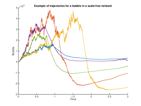
Figure 2: Scale-free network.

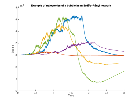
Figure 3: Erdős-Rényi network.

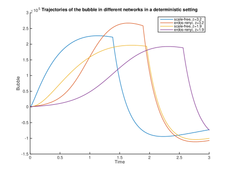
Figure 4: Deterministic example.