An integral equation-based numerical solver for Taylor states in toroidal geometries

Abstract

We present an algorithm for the numerical calculation of Taylor states in toroidal and toroidal-shell geometries using an analytical framework developed for the solution to the time-harmonic Maxwell equations. Taylor states are a special case of what are known as Beltrami fields, or linear force-free fields. The scheme of this work relies on the generalized Debye source representation of Maxwell fields and an integral representation of Beltrami fields which immediately yields a well-conditioned second-kind integral equation. This integral equation has a unique solution whenever the Beltrami parameter $\lambda$ is not a member of a discrete, countable set of resonances which physically correspond to spontaneous symmetry breaking. Several numerical examples relevant to magnetohydrodynamic equilibria calculations are provided. Lastly, our approach easily generalizes to arbitrary geometries, both bounded and unbounded, and of varying genus.

Keywords: Beltrami field, Beltrami flow, generalized Debye sources, time-harmonic Maxwell’s equations, plasma physics, electromagnetics, Debye sources, force-free fields, Taylor states, magnetohydrodynamics

1 Introduction

A wide range of astrophysical and laboratory plasmas are in force-free equilibria [27, 2, 51, 55] where the magnetic field $\bm{B}$ satisfies

$$(\nabla\times\bm{B})\times\bm{B}=\bm{0}$$ (1.1)

This immediately implies that the current density $\bm{J}=(\nabla\times\bm{B})/\mu_{0}$ is parallel to the magnetic field, i.e. there exists a scalar function $\lambda=\lambda(\bm{x})$ such that

$$\nabla\times\bm{B}=\lambda\bm{B}.$$ (1.2)

Within the general class of linear force-free equilibria described by (1.2), Taylor states or Woltjer-Taylor states are particular equilibria for which $\lambda$ is a spatially uniform constant given by the ratio of the magnetic energy to the magnetic helicity, see Chapter 11 of [6]. They play a central role in plasma physics [15, 59, 11, 54, 21, 5, 40, 22] as the natural state resulting from dissipative turbulent relaxation [55, 50]. Since they satisfy the equation $\nabla\times\bm{B}=\lambda\bm{B}$ with $\lambda$ constant, magnetic fields in Taylor state configurations are a special case of a class of force-free fields called linear Beltrami fields [3, 7]. Since in this work we will consider $\lambda$ to be a given input to the solver, we will use the expressions Taylor state and linear Beltrami field interchangeably for the remainder of this article.

Linear Beltrami fields have been extensively studied mathematically, and their properties are well understood by now [39, 49, 25, 43, 19]. On the other hand, relatively few numerical solvers have been developed to compute them in geometries relevant to plasma physics. To the best of the authors’ knowledge, solvers for these problems based on integral equation formulations have never been constructed despite their desirable properties: access to relatively high-precision derivatives of the field (via analytic differentiation of the integral representation), low memory requirements (only the boundary has to be discretized), and overall rapid convergence of the solution (when coupled with high-order quadrature rules and a fast algorithm, such as a fast multipole method).

We take a moment to justify this claim. One may at first think that Taylor states in axisymmetric toroidal geometries can be viewed as a special class of more general Grad-Shafranov equilibria [32, 52], as was for instance done in [14]. From this point of view, Grad-Shafranov solvers relying on integral formulations [44, 48] could be used to compute linear Beltrami fields. However, this approach is not satisfactory for the following reasons. First, a Grad-Shafranov solver would not take advantage of the particular properties of linear Beltrami fields. Second, certain applications [11, 40] require the computation of linear Beltrami fields in hollow toroidal shells. Grad-Shafranov solvers are usually not designed to handle such geometries. Finally, and most importantly, Taylor states in axisymmetric domains may not be axisymmetric themselves [55]. By definition, the Grad-Shafranov equation does not apply to these fully three-dimensional, bifurcated states.

The purpose of this article is to present the first integral equation solver for the calculation of Taylor states in toroidal regions. While preliminary results from this work were given in [25], details of the actual solver were not provided. A separation of variables numerical solver for the full exterior axisymmetric electromagnetic scattering problem from perfect conductors is discussed in [26], but this work does not address the computation of interior eigenfunctions nor solve the boundary value problem with data on the normal components of $\bm{E}$, $\bm{H}$. We close this gap with the present work. The integral formulation we present here applies to both toroidally axisymmetric and non-axisymmetric domains, but thus far our numerical solver can only treat the first situation. We will therefore restrict the description of the numerical solver to that case. Let us stress again that while the domain is axisymmetric, the Taylor state itself may not be, and the solver we present here can compute these non-axisymmetric equilibria. As such, it may be applied to the computation of magnetohydrodynamic equilibria in spheromaks [29], reversed field pinches [56], and in tokamaks for start-up scenarios [5] and the study of magnetohydrodynamic instabilities [34, 31].

The mathematically well-posed form of the problem is as follows. We construct numerical solutions to the Beltrami boundary-value problem given by:

$$\nabla\times\bm{B} =\lambda\bm{B} \text{in }\Omega,$$ (1.3)

$$\bm{B}\cdot\bm{\mathsf{n}} =0 \text{on }\Gamma,$$

where $\lambda$ is a real number given as input to the solver, $\Omega$ is an axisymmetric toroidal domain, and $\Gamma=\partial\Omega$ is the (smooth) boundary of the region $\Omega$. Depending on the genus of $\Gamma$, additional (topological) constraints on $\bm{B}$ must be added in order for (1.3) to be well-posed. For Taylor states in laboratory plasmas, it is often natural to take these constraints as conditions on the toroidal and poloidal flux of $\bm{B}$ [55, 40], see Figure 1(a). In a genus-two toroidal flux shell (see Figure 1(b)) two conditions must be imposed:

$$\int_{S_{t}}\bm{B}\cdot d\bm{a}=\Phi^{\text{tor}}\qquad\text{and}\qquad\int_{S_{p}}\bm{B}\cdot d\bm{a}=\Phi^{\text{pol}},$$ (1.4)

where $d\bm{a}=\bm{\mathsf{n}}\,da$, with $da$ being the surface area element and $\bm{\mathsf{n}}$ the oriented normal along the surfaces $S_{t}$ and $S_{p}$. On the other hand, if the toroidal domain is not hollow (genus-one), only one additional flux condition is necessary. The need for extra conditions (1.4) to ensure well-posedness stems from the multiply-connectedness of the boundary $\Gamma$ – namely, the existence of harmonic surface vector fields on $\Gamma$ and interior volume $\lambda$-Neumann vector fields in $\Omega$ [23]. Readers interested in more details on the well-posedness of the boundary value problem (1.3, 1.4) may read references [43, 25].

Our integral equation formulation is based on the observation that if $\nabla\times\bm{B}=\lambda\bm{B}$, then the pair $\{\bm{E},\bm{H}\}=\{i\bm{B},\bm{B}\}$ satisfies the time-harmonic Maxwell’s equations in vacuum, with $\lambda$ playing the role of a wavenumber. Boundary conditions on the normal component of $\bm{B}$ then correspond to boundary conditions on the normal components of $\bm{E}$ and $\bm{H}$. This fact, coupled with the symmetry of $\bm{E}$ and $\bm{H}$, makes it natural to represent $\bm{B}$ using generalized Debye sources, as in [23, 25]. Application of the boundary condition in (1.3) and flux constraints (1.4) to the generalized Debye source representation immediately yields a second-kind integral equation which can be solved with standard techniques.

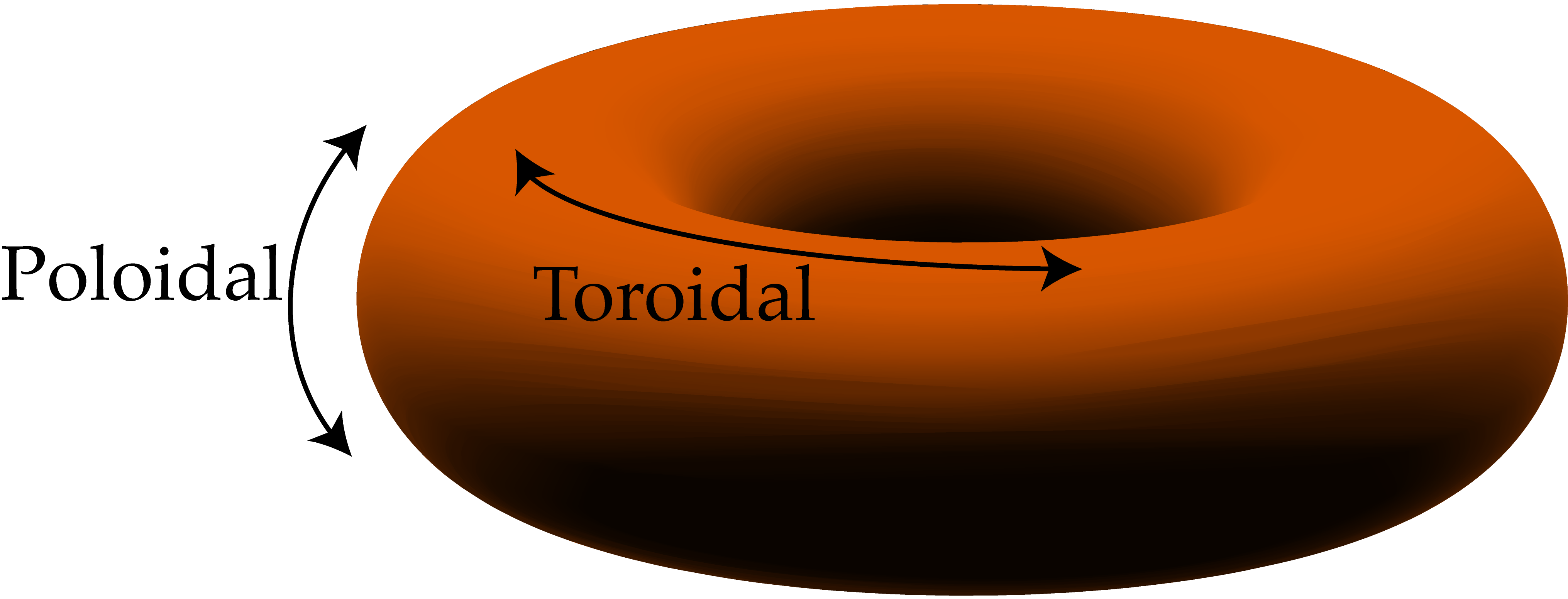
(a) Poloidal and toroidal directions.

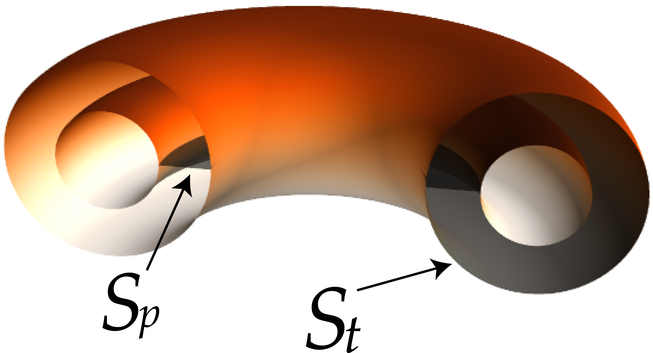
(b) Genus-two toroidal shell.

Figure 1: The basic geometry of the toroidal domains relevant to axisymmetric magnetohydrodynamics. The boundary $\Gamma$ of the domain is shown in orange shading, while the surfaces $S_{t}$ and $S_{p}$ on which the magnetic fluxes are specified are shown in gray shading.

The paper is organized as follows. In Section 2, we establish the link between linear Beltrami fields and the generalized Debye representation at the heart of our integral equation formulation. In Sections 3 and 4, we derive the second-kind integral equations for the densities of the vector and scalar potentials in the generalized Debye representation of the Beltrami field. Section 3 applies to toroidal regions, while Section 4 applies to hollow toroidal shells. Section 5 describes our numerical method to compute the solution to the integral equations, and to subsequently evaluate the Beltrami fields. In Section 6, we illustrate the flexibility and accuracy of our solver with three examples that are relevant to laboratory plasma experiments, and in Section 7 we summarize our work and discuss ideas for further development.

2 Beltrami fields and the generalized Debye source representation

In this section, we introduce the generalized Debye source representation of linear Beltrami fields. The generalized Debye source representation was originally developed for solving time-harmonic electromagnetic scattering problems from perfect electric conductors and dielectric materials [23, 24], but has recently been found to be extremely well-suited for describing force-free fields with spatially constant Beltrami parameter $\lambda$ [25]. The representation immediately leads to a well-conditioned (away from physical interior resonances) second-kind integral equation which can be numerically inverted to high-precision. We first present the generalized Debye representation for the time-harmonic Maxwell equations, and then make the connection with linear Beltrami fields.

2.1 Debye source representation for time-harmonic Maxwell’s equations

In their simplest form, the time-harmonic Maxwell’s equations in a region free of charge and current, are given by:

$$\nabla\times\bm{E} =ik\bm{H}\qquad \nabla\times\bm{H} =-ik\bm{E}$$ (2.1)

$$\nabla\cdot\bm{E} =0 \nabla\cdot\bm{H} =0,$$

where $\bm{E}$ and $\bm{H}$ are the electric and magnetic fields, respectively, and have been suitably scaled by the electric permittivity and magnetic permeability so that the equations only depend on a single parameter, $k$. The real wavenumber $k$ is proportional to the time-harmonic angular frequency $\omega$, with $k=\omega/2\pi$. Epstein and Greengard have recently developed a new and robust integral representation for the solution to (2.1) in the exterior of objects with smooth boundaries for the standard perfect electric conductor homogeneous boundary conditions on $\bm{E}$ and $\bm{H}$ [23]:

$$\bm{\mathsf{n}}\times\bm{E}=0,\qquad\bm{\mathsf{n}}\cdot\bm{H}=0.$$ (2.2)

This representation, called the generalized Debye source representation, is a full potential-antipotential formulation, given by:

$$\bm{E} =ik\bm{A}-\nabla u-\nabla\times\bm{Q},$$ (2.3)

$$\bm{H} =ik\bm{Q}-\nabla v+\nabla\times\bm{A},$$

along with the two consistency conditions on the potentials

$$\nabla\cdot\bm{A}=iku,\qquad\nabla\cdot\bm{Q}=ikv.$$ (2.4)

In the exterior of a scatterer with smooth closed boundary $\Gamma$, the vector and scalar potentials are constructed as

$$\bm{A}(\bm{x}) =\int_{\Gamma}\frac{e^{ik|\bm{x}-\bm{x}^{\prime}|}}{4\pi|\bm{x}-\bm{x}^{\prime}|}\,\bm{j}(\bm{x}^{\prime})\,da(\bm{x}^{\prime}), \qquad\bm{Q}(\bm{x}) =\int_{\Gamma}\frac{e^{ik|\bm{x}-\bm{x}^{\prime}|}}{4\pi|\bm{x}-\bm{x}^{\prime}|}\,\bm{m}(\bm{x}^{\prime})\,da(\bm{x}^{\prime}),$$ (2.5)

$$u(\bm{x}) =\int_{\Gamma}\frac{e^{ik|\bm{x}-\bm{x}^{\prime}|}}{4\pi|\bm{x}-\bm{x}^{\prime}|}\,\rho(\bm{x}^{\prime})\,da(\bm{x}^{\prime}), v(\bm{x}) =\int_{\Gamma}\frac{e^{ik|\bm{x}-\bm{x}^{\prime}|}}{4\pi|\bm{x}-\bm{x}^{\prime}|}\,\sigma(\bm{x}^{\prime})\,da(\bm{x}^{\prime}),$$

where $da(\bm{x}^{\prime})$ denotes the surface area differential along $\Gamma$ at the point $\bm{x}^{\prime}$, and the kernel is the Green’s function for the Helmholtz equation in three dimensions (Chapter 2 of [46]):

$$g(\bm{x},\bm{x}^{\prime})=\frac{e^{ik|\bm{x}-\bm{x}^{\prime}|}}{4\pi|\bm{x}-\bm{x}^{\prime}|}.$$ (2.6)

In order for the consistency conditions (2.4) to be satisfied, it must be the case that [23]

$$\nabla_{\Gamma}\cdot\bm{j}=ik\rho,\quad\text{and}\quad\nabla_{\Gamma}\cdot\bm{m}=ik\sigma,$$ (2.7)

where $\nabla_{\Gamma}\cdot\bm{F}$ denotes the intrinsic surface divergence of a tangent vector field $\bm{F}$ along $\Gamma$. When the scattering object is a perfect conductor, the surface vector fields $\bm{j}$, $\bm{m}$ are written as

$$\bm{j} =ik\left(\nabla_{\Gamma}\Delta_{\Gamma}^{-1}\rho-\bm{\mathsf{n}}\times\nabla_{\Gamma}\Delta_{\Gamma}^{-1}\sigma\right)+\bm{j}_{H}$$ (2.8)

$$\bm{m} =ik\left(\nabla_{\Gamma}\Delta_{\Gamma}^{-1}\sigma+\bm{\mathsf{n}}\times\nabla_{\Gamma}\Delta_{\Gamma}^{-1}\rho\right)+\bm{m}_{H}$$

$$=\bm{\mathsf{n}}\times\bm{j},$$

and automatically satisfy (2.7). Here $\nabla_{\Gamma}$ is the surface gradient operator, and by $\Delta_{\Gamma}^{-1}$ we denote the inverse of the surface Laplacian (Laplace-Beltrami operator) along $\Gamma$ restricted to the class of mean-zero functions. That is to say, the generalized Debye sources $\rho$, $\sigma$ are required to have mean zero, as well as the functions $\alpha=\Delta_{\Gamma}^{-1}\rho$ and $\beta=\Delta_{\Gamma}^{-1}\sigma$. Restricted to the class of mean-zero functions defined on $\Gamma$, the Laplace-Beltrami operator is uniquely invertible [23]. Furthermore, the surface vector fields $\bm{j}_{H}$ and $\bm{m}_{H}$ are harmonic, in the sense that

$$\nabla_{\Gamma}\cdot\bm{j}_{H}=0,\qquad\nabla_{\Gamma}\cdot\bm{\mathsf{n}}\times\bm{j}_{H}=0,$$ (2.9)

and likewise for $\bm{m}_{H}$. The construction of $\bm{j}$, $\bm{m}$ in (2.8) ensures uniqueness of the underlying representation.

This concludes the overview of the generalized Debye source representation that we will use in the remainder of the paper. More details regarding the simulation of time-harmonic Maxwell fields using the generalized Debye source approach can be found in [23, 24, 26]. We are now ready to turn to the problem of interest, namely the construction of an integral representation for linear Beltrami fields based on the generalized Debye representation. We start by highlighting the link between the scattering problem discussed above and linear Beltrami fields.

2.2 Generalized Debye representation for linear Beltrami fields

We want to compute, for a given $\lambda\geq 0$, the magnetic field $\bm{B}$ satisfying

$$\nabla\times\bm{B} =\lambda\bm{B} \text{in }\Omega,$$ (2.10)

$$\bm{B}\cdot\bm{\mathsf{n}} =0 \text{on }\Gamma,$$

where $\Omega$ is an axisymmetric toroidal domain, and $\Gamma=\partial\Omega$ is the boundary of $\Omega$. Note that as stated here, (2.10) does not have a unique solution. For uniqueness, additional constraints must be imposed on $\bm{B}$, which we will take to be constraints on the magnetic flux, as already discussed in the introduction. We will return to this point in Sections 3 and 4, where we construct the integral equations used by our solver.

Now, assume that $\bm{B}$ satisfies (2.10). Then the pair $\{\bm{E}$,$\bm{H}\}$ given by

$$\bm{E}=i\bm{B},\quad\text{and}\quad\bm{H}=\bm{B}.$$ (2.11)

satisfies Maxwell’s equations (2.1), with $\lambda$ playing the role of $k$ and the boundary conditions $\bm{E}\cdot\bm{\mathsf{n}}=0$ and $\bm{H}\cdot\bm{\mathsf{n}}=0$ on $\Gamma$. Analysis of this interior boundary value problem was done in 1986 by Kress [42], and later discussed with regard generalized Debye sources and the Beltrami problem in 2015 [25], but no detailed computations were performed. With this in mind, motivated by the specific relationship $\bm{E}=i\bm{H}$, the symmetry of the generalized Debye representation provides a natural representation for the Maxwell pair $\{\bm{E}$,$\bm{H}\}$: the vector and scalar potentials must satisfy [24]

$$\bm{A}=i\bm{Q}\quad\text{and}\quad u=iv.$$ (2.12)

The relationship above is required for Beltrami fields in the interior or exterior of $\Gamma$, otherwise $\nabla\times\bm{B}=\lambda\bm{B}$ is not satisfied. We thus represent our force-free field $\bm{B}$ as

$$\bm{B}=i\lambda\bm{Q}-\nabla v+i\,\nabla\times\bm{Q},$$ (2.13)

where $\bm{Q}$ and $v$ are generalized Debye potentials for boundary conditions associated with the magnetic field along a perfect conductor.

We now turn our attention to the particular representation that we will use for Beltrami fields in the interior of genus-one tori and genus-two toroidal shells, i.e. the exact construction of the surface vector field $\bm{m}$ introduced above, following the presentation given in Section 2.1. The expressions for the case of genus-one tori and of genus-two toroidal shells differ slightly on several occasions, so we treat each case in a separate section.

3 Beltrami fields in toroidal geometries

In the previous section, the generalized Debye source representation was shown to be a natural way to represent Beltrami fields because of the inherent symmetry between the electric and magnetic fields. In this section, we provide the exact construction of the surface vector field $\bm{m}$ as well as derive a second-kind integral equation which is uniquely invertible except when the Beltrami parameter $\lambda$ is precisely an eigenvalue of the curl operator [25].

As explained in the previous section, in the interior of a genus-one torus we will represent Beltrami fields as

$$\bm{B}=i\lambda\bm{Q}-\nabla v+i\,\nabla\times\bm{Q},$$ (3.1)

where $\bm{Q}$ and $v$ are vector and scalar potentials, respectively, given by layer potentials along $\Gamma$, the boundary of a toroidal region $\Omega$:

$$\bm{Q}(\bm{x})=\int_{\Gamma}g(\bm{x},\bm{x}^{\prime})\,\bm{m}(\bm{x}^{\prime})\,da(\bm{x}^{\prime}),\qquad v(\bm{x})=\int_{\Gamma}g(\bm{x},\bm{x}^{\prime})\,\sigma(\bm{x}^{\prime})\,da(\bm{x}^{\prime}).$$ (3.2)

In order for $\bm{B}$ to satisfy Beltrami’s equation (and for the pair $\{i\bm{B}$, $\bm{B}\}$ to satisfy Maxwell’s equations) it is necessary that

$$\nabla_{\Gamma}\cdot\bm{m}=i\lambda\sigma.$$ (3.3)

We now provide an explicit construction of $\bm{m}$ in terms of $\sigma$ and a harmonic surface vector field $\bm{m}_{H}$ such that the representation is unique and leads to an invertible integral equation. To this end, let us assume that all differential surface operators are oriented with respect to a unit normal vector $\bm{\mathsf{n}}$ along $\Gamma$ which is always assumed to point into the region $\Omega^{c}$, the complement of $\Omega$ (i.e. the unit outward normal). As described in Section 2.1, the surface vector field $\bm{m}$ given by

$$\bm{m}=i\lambda\left(\nabla_{\Gamma}\Delta_{\Gamma}^{-1}\sigma-i\,\bm{\mathsf{n}}\times\nabla_{\Gamma}\Delta_{\Gamma}^{-1}\sigma\right)+\alpha\,\bm{m}_{H}.$$ (3.4)

is constructed to automatically enforce the consistency condition (3.3) and yield uniqueness in the resulting integral equation, derived below, in (3.7). The surface vector field $\bm{m}_{H}$ appearing in expression (3.4) is a tangential harmonic vector field satisfying the conditions:

$$\begin{gathered}\nabla_{\Gamma}\cdot\bm{m}_{H}=0,\qquad\quad\nabla_{\Gamma}\cdot\bm{\mathsf{n}}\times\bm{m}_{H}=0,\\ \bm{\mathsf{n}}\times\bm{m}_{H}=i\,\bm{m}_{H}.\end{gathered}$$ (3.5)

The constant $\alpha$ appearing in front of $\bm{m}_{H}$ is a complex number to be determined in the solution of the Beltrami boundary-value problem. The relationship between $\bm{\mathsf{n}}\times\bm{m}_{H}$ and $\bm{m}_{H}$ is in fact necessary in order to ensure uniqueness of the integral representation [25], and is analogous to the relationship between $\bm{A}$ and $\bm{Q}$ in (2.12).

Using this representation for $\bm{B}$, it is straightforward to derive a second-kind integral equation (augmented with flux conditions) for the unknowns $\sigma$ and $\alpha$ by merely enforcing the local boundary condition $\bm{B}\cdot\bm{\mathsf{n}}=0$ and global integral constraint. Introducing the single-layer operator $\mathcal{S}$ as

$$\mathcal{S}[f](\bm{x})=\int_{\Gamma}g(\bm{x},\bm{x}^{\prime})\,f(\bm{x}^{\prime})\,da(\bm{x}^{\prime}),$$ (3.6)

the integral equation and flux condition can be written as

$$\frac{\sigma}{2}+\mathcal{K}[\sigma,\alpha] =0,$$ (3.7)

$$\int_{S_{t}}\bm{B}(\sigma,\alpha)\cdot d\bm{a} =\Phi^{\text{tor}},$$

where $d\bm{a}=\bm{\mathsf{n}}\,da$ and with the notation $\bm{B}(\sigma,\alpha)$ we highlight the fact that the magnetic field $\bm{B}$ is a function of $\sigma$ and $\alpha$. In (3.7) the operator $\mathcal{K}$ has been used to abbreviate the compact operator

$$\mathcal{K}[\sigma,\alpha]=i\lambda\,\bm{\mathsf{n}}\cdot\mathcal{S}[\bm{m}]-\mathcal{\mathcal{S}}^{\prime}[\sigma]+i\,\bm{\mathsf{n}}\cdot\nabla\times\mathcal{S}[\bm{m}],$$ (3.8)

where $\bm{m}=\bm{m}(\sigma,\alpha)$ as in (3.4), and $\mathcal{S}^{\prime}$ is the normal derivative of the single-layer potential, interpreted in the appropriate principal-value sense (Chapter 2 of [18]). The flux condition in system (3.7) is still not optimal from the point of view of a boundary integral equation because the integration is being carried out over an additional surface $S_{t}$ (depicted in Figure 1(b)) spanning the cross section of the toroidal region $\Omega$. Letting $\partial S_{t}$ denote the curve bounding this surface, $\partial S_{t}=\Gamma\cap S_{t}$, we can reduce this flux integral to a circulation integral using Stokes’ theorem and the fact that $\bm{B}$ is a Beltrami field:

$$\int_{S_{t}}\bm{B}\cdot d\bm{a} =\int_{S_{t}}\frac{1}{\lambda}(\nabla\times\bm{B})\cdot d\bm{a},$$ (3.9)

$$=\frac{1}{\lambda}\int_{\partial S_{t}}\bm{B}\cdot d\bm{l},$$

where $d\bm{l}$ denotes the unit arclength differential. For small values of $\lambda$, special care must be taken in numerically evaluating this integral, as discussed in Section 5 of [24].

We now turn our attention to deriving an analogous representation for Beltrami fields in genus-two toroidal shells. The only difference with the present situation is the inclusion of an extra surface harmonic vector field because of the genus of the boundary. For this reason, two integral (flux) constraints must be enforced to construct a well-posed boundary-value problem, as opposed to the single condition enforced in this section.

4 Beltrami fields in toroidal shells

In this section, we extend the representation of Beltrami fields introduced in the previous section to toroidal geometries with genus two. Specifically, we turn our attention to geometries which are topologically equivalent to that in Figure 1(b), which from now on we will refer to as a toroidal shell. The viability of this extension to geometries whose boundary consists of more than one component is discussed in [25]. The following discussion makes one minor change in notation from the previous section: the interior of the genus-two toroidal shell is still given by $\Omega$, however its boundary $\Gamma$ is now explicitly given by the union of two disjoint boundaries, $\Gamma=\Gamma^{\text{out}}\cup\Gamma^{\text{in}}$. The unbounded component of $\Omega^{c}$ is assumed to be bounded by $\Gamma^{\text{out}}$ and the bounded component is assumed to be bounded by $\Gamma^{\text{in}}$. We assume that the unit normal $\bm{\mathsf{n}}$ along $\Gamma^{\text{out}}$ points into the unbounded component of $\Omega^{c}$, but that the unit normal $\bm{\mathsf{n}}$ along $\Gamma^{\text{in}}$ points into $\Omega$. This convention may be non-standard, but it treats each surface as having the same counter-clockwise parameterization and simplifies implementation details.

The representation for Beltrami fields in $\Omega$ given by (3.1) does not change, however the construction of the surface vector field $\bm{m}$ is altered slightly to account for the disjoint boundaries. In the genus-two case, the vector field $\bm{m}$ consists of two components, $\bm{m}^{\text{out}}$ defined along $\Gamma^{\text{out}}$ and $\bm{m}^{\text{in}}$ defined along $\Gamma^{\text{in}}$:

$$\bm{m}=\begin{cases}i\lambda\left(\nabla_{\Gamma}\Delta_{\Gamma}^{-1}\sigma-i\,\bm{\mathsf{n}}\times\nabla_{\Gamma}\Delta_{\Gamma}^{-1}\sigma\right)+\alpha\,\bm{m}^{\text{out}}_{H}&\qquad\text{on }\Gamma^{\text{out}},\\ i\lambda\left(\nabla_{\Gamma}\Delta_{\Gamma}^{-1}\sigma+i\,\bm{\mathsf{n}}\times\nabla_{\Gamma}\Delta_{\Gamma}^{-1}\sigma\right)+\beta\,\bm{m}^{\text{in}}_{H}&\qquad\text{on }\Gamma^{\text{in}},\end{cases}$$ (4.1)

where the harmonic surface vector fields $\bm{m}^{\text{out}}_{H}$ and $\bm{m}^{\text{in}}_{H}$ (which are only defined on $\Gamma^{\text{out}}$ and $\Gamma^{\text{in}}$, respectively) must satisfy:

$$\bm{\mathsf{n}}\times\bm{m}_{H}^{\text{out}} =i\bm{m}^{\text{out}}_{H},$$ (4.2)

$$\bm{\mathsf{n}}\times\bm{m}_{H}^{\text{in}} =-i\,\bm{m}^{\text{in}}_{H}.$$

The difference in these relationships is due to the fact that the Beltrami field in $\Omega$ appears as an exterior field from the point of view of $\Gamma^{\text{in}}$. As in the previous section, enforcing the boundary conditions

$$\begin{gathered}\bm{B}\cdot\bm{\mathsf{n}}=0\qquad\text{on }\Gamma,\\ \int_{S_{t}}\bm{B}\cdot d\bm{a}=\Phi^{\text{tor}},\qquad\int_{S_{p}}\bm{B}\cdot d\bm{a}=\Phi^{\text{pol}}\end{gathered}$$ (4.3)

yields an augmented second-kind integral equation for $\sigma$, $\alpha$, and $\beta$ which is similar to the previous situation:

$$\frac{1}{2}\sigma^{\text{out}}+\mathcal{K}[\sigma,\alpha,\beta] =0, \text{on }\Gamma^{\text{out}},$$ (4.4)

$$-\frac{1}{2}\sigma^{\text{in}}+\mathcal{K}[\sigma,\alpha,\beta] =0, \text{on }\Gamma^{\text{in}},$$

$$\int_{S_{t}}\bm{B}(\sigma,\alpha,\beta)\cdot d\bm{a} =\Phi^{\text{tor}},$$

$$\int_{S_{p}}\bm{B}(\sigma,\alpha,\beta)\cdot d\bm{a} =\Phi^{\text{pol}},$$

where we have once more emphasized that the magnetic field $\bm{B}$ is expressed in terms of $\sigma$, $\alpha$ and $\beta$ and where we have explicitly shown the dependence on densities $\sigma^{\text{out}}$, $\sigma^{\text{in}}$ which are defined along $\Gamma^{\text{out}}$ and $\Gamma^{\text{in}}$, respectively, to highlight the change of sign on the diagonal. The compact operator $\mathcal{K}$ is as before,

$$\mathcal{K}[\sigma,\alpha,\beta]=i\lambda\,\bm{\mathsf{n}}\cdot\mathcal{S}[\bm{m}]-\mathcal{S}^{\prime}[\sigma]+i\,\bm{\mathsf{n}}\cdot\nabla\times\mathcal{S}[\bm{m}].$$ (4.5)

except that we have to keep in mind that the operator has contributions from densities on both $\Gamma^{\text{out}}$ and $\Gamma^{\text{in}}$. The flux surface integrals in (4.4) can be written as circulation integrals on $\Gamma^{\text{out}}$ and $\Gamma^{\text{in}}$ by invoking Stokes’ Theorem:

$$\int_{S_{t}}\bm{B}\cdot d\bm{a}=\frac{1}{\lambda}\int_{\partial S_{1}}\bm{B}\cdot d\bm{l},\qquad\int_{S_{p}}\bm{B}\cdot d\bm{a}=\frac{1}{\lambda}\int_{\partial S_{2}}\bm{B}\cdot d\bm{l},$$ (4.6)

where the line integrals are on the closed curves $\partial S_{1}=\Gamma\cap S_{t}$ and $\partial S_{2}=\Gamma\cap S_{t}$. Both of these flux integrals can be computed as the difference of circulation integrals, the former around what are known as $B$-cycles and the latter around $A$-cycles, see Figure 2. We describe the actual numerical calculation of these integrals in Section 5.

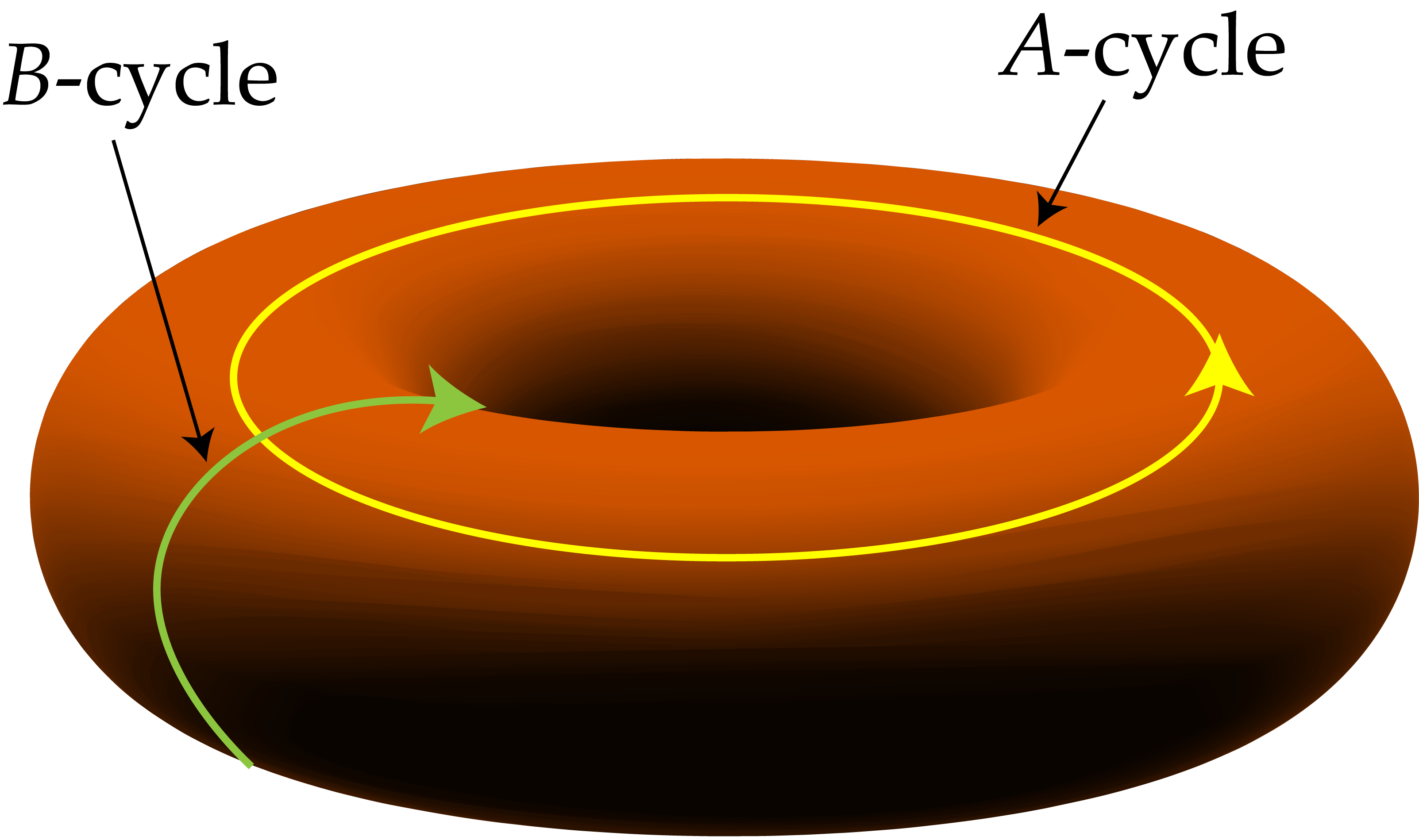
Figure 2: $A$- and $B$-cycles along a toroidal boundary.

5 An axisymmetric integral equation solver

In this section we describe the numerical implementation of the integral equation solver we have developed to calculate force-free Beltrami fields in toroidally axisymmetric geometries. A similar version of this solver, optimized for full electromagnetic multi-mode calculations, appears in [26]. Related to this work are the very efficient scalar axisymmetric solvers for the Laplace and Helmholtz equations presented in [60, 37, 36, 35]. In the following discussion, we assume that a point $\bm{x}\in\mathbb{R}^{3}$ has cylindrical coordinates given by $\bm{x}=(x,y,z)=(r\cos\phi,r\sin\phi,z)$, where $r$ represents the distance from the axis of revolution, and $\phi$ is the toroidal angle. The orthonormal unit vectors in Cartesian coordinates will be denoted $\bm{\mathsf{i}}$, $\bm{\mathsf{j}}$, $\bm{\mathsf{k}}$, and the orthonormal unit vectors in cylindrical coordinates will be denoted in bold-face as $\bm{\mathsf{r}}$, $\bm{\phi}$, $\bm{\mathsf{z}}$. The Cartesian and cylindrical bases are related through

$$\bm{\mathsf{r}}(\phi) =\cos\phi\,\bm{\mathsf{i}}+\sin\phi\,\bm{\mathsf{j}}, \qquad\bm{\mathsf{i}} =\cos\phi\,\bm{\mathsf{r}}(\phi)-\sin\phi\,\bm{\phi}(\phi),$$ (5.1)

$$\bm{\phi}(\phi) =-\sin\phi\,\bm{\mathsf{i}}+\cos\phi\,\bm{\mathsf{j}}, \qquad\bm{\mathsf{j}} =\sin\phi\,\bm{\mathsf{r}}(\phi)+\cos\phi\,\bm{\phi}(\phi),$$

$$\bm{\mathsf{z}} =\bm{\mathsf{k}}, \bm{\mathsf{k}} =\bm{\mathsf{z}},$$

These relationships will be useful in the following sections. The following addition formulae will also be useful:

$$\bm{\mathsf{r}}(\phi-\phi^{\prime}) =\cos\phi^{\prime}\,\bm{\mathsf{r}}(\phi)-\sin\phi^{\prime}\,\bm{\phi}(\phi)$$ (5.2)

$$\bm{\phi}(\phi-\phi^{\prime}) =\sin\phi^{\prime}\,\bm{\mathsf{r}}(\phi)+\cos\phi^{\prime}\,\bm{\phi}(\phi)$$

The dependence of $\bm{\mathsf{r}}$ and $\bm{\phi}$ on $\phi$ will be dropped when unnecessary.

We now revisit some earlier notation. Let $\Omega$, as before, be a toroidally axisymmetric domain in $\mathbb{R}^{3}$ with boundary $\Gamma$. That is to say, rotation about the $z$-axis does not alter $\Omega$. The boundary of the $\phi=0$ cross-section of $\Omega$ in the $xz$-plane (and the $rz$-plane in cylindrical coordinates) will be denoted by $\gamma$, and will be referred to as the generating curve for $\Gamma$, see Figure 3(b). Note that in the $\phi=0$ plane,

$$\bm{\mathsf{r}}=\bm{\mathsf{i}},\quad\bm{\phi}=\bm{\mathsf{j}},\quad\bm{\mathsf{z}}=\bm{\mathsf{k}}.$$ (5.3)

In a minor abuse of notation, we will assume that the curve $\gamma:[0,L]\to\mathbb{R}^{2}$ is parameterized by functions $r(s)$, $z(s)$ of the arc length $s$:

$$\gamma(s)=(r(s),z(s)),$$ (5.4)

and therefore $|d\gamma/ds|=1$. Any point $\bm{x}\in\Gamma$ is given as

$$\bm{x}(s,\phi)=r(s)\cos\phi\,\bm{\mathsf{i}}+r(s)\sin\phi\,\bm{\mathsf{j}}+z(s)\bm{\mathsf{k}}.$$ (5.5)

Furthermore, we will assume that $\gamma$ is positively oriented such that the unit normal along $\Gamma$, given by

$$\bm{\mathsf{n}}=\frac{dz}{ds}\bm{\mathsf{r}}-\frac{dr}{ds}\bm{\mathsf{z}},$$ (5.6)

points into $\Omega^{c}$. Note that $\bm{\mathsf{n}}=\bm{\mathsf{n}}(s,\phi)$. Along the boundary $\Gamma$, it will be useful to work in a system of local coordinates $\bm{\tau}$, $\bm{\phi}$, $\bm{\mathsf{n}}$, shown in Figure 3(a). Relative to the coordinate system given by $\bm{\mathsf{r}}$, $\bm{\phi}$, $\bm{\mathsf{z}}$, the unit vector $\bm{\tau}$ along $\Gamma$ is given by

$$\bm{\tau}=\frac{dr}{ds}\bm{\mathsf{r}}+\frac{dz}{ds}\bm{\mathsf{z}}.$$ (5.7)

This local coordinate system satisfies the relation $\bm{\mathsf{n}}=\bm{\phi}\times\bm{\tau}$.

(a) Local surface coordinate system along $\Gamma^{\text{out}}$.

(b) Generating curves for toroidal shells.

Figure 3: Geometry parameterization. The shell $\Gamma$ is shaded in orange, and the generating curve is drawn in black in Figure 3(b).

We start the description of the numerical implementation by explaining how the surface integral equation naturally separates into Fourier modes, as was already shown in a different context in [60], and how the vector potential can be decomposed into Fourier modes.

5.1 Separation into Fourier modes

For any integral equation on an axisymmetric surface $\Gamma$ whose kernel $g(\bm{x},\bm{x}^{\prime})$ only depends on the quantity $\phi-\phi^{\prime}$, i.e. $g(\bm{x},\bm{x}^{\prime})=g(r,z,r^{\prime},z^{\prime},\phi-\phi^{\prime})$ one may Fourier transform the surface integral equation on $\Gamma$ into a series of decoupled integral equations along its generating curve $\gamma$. In what follows, for clarity we will use the notation:

$$g(s,s^{\prime},\phi-\phi^{\prime}) =g(r(s),z(s),r(s^{\prime}),z(s^{\prime}),\phi-\phi^{\prime}).$$ (5.8)

Since any point on $\Gamma$ is given as $\bm{x}=(r(s),\phi,z(s))$, the solution $\sigma$ to

$$\sigma(\bm{x})+\int_{\Gamma}g(\bm{x},\bm{x}^{\prime})\,\sigma(\bm{x}^{\prime})\,da(\bm{x}^{\prime})=f(\bm{x})$$ (5.9)

can be written as

$$\sigma(s,\phi)=\sum_{\ell}\sigma_{\ell}(s)\,e^{i\ell\phi}.$$ (5.10)

The functions $\sigma_{\ell}$ are the solution to a series of uncoupled integral equations on $\gamma$:

$$\sigma_{\ell}(s)+2\pi\int_{\gamma}g_{\ell}(s,s^{\prime})\,\sigma_{\ell}(s^{\prime})\,r(s^{\prime})\,ds^{\prime}=f_{\ell}(s),$$ (5.11)

with the kernels $g_{\ell}$ and right hand sides $f_{\ell}$ given by:

$$g_{\ell}(s,s^{\prime}) =\frac{1}{2\pi}\int_{-\pi}^{\pi}g(s,s^{\prime},\phi)\,e^{-i\ell\phi}\,d\phi,$$ (5.12)

$$f_{\ell}(s) =\frac{1}{2\pi}\int_{-\pi}^{\pi}f(s,\phi)\,e^{-i\ell\phi}\,d\phi.$$

It now remains to see how one writes the Fourier mode of the vector potential $\bm{Q}$ given by (3.2). This requires computing the Fourier modes of a layer potential applied to a tangential vector-field, $\bm{u}$. To this end, consider the following integral along $\Gamma$ for the tangent vector field $\bm{u}$:

$$\int_{\Gamma}g(\bm{x},\bm{x}^{\prime})\,\bm{u}(\bm{x}^{\prime})\,da(\bm{x}^{\prime}),$$ (5.13)

where $\bm{u}$ is given by:

$$\bm{u}=u^{\tau}\bm{\tau}+u^{\phi}\bm{\phi}$$ (5.14)

Since $\Gamma$ is a surface of revolution, the tangential vector field in (5.14) can be written in terms of its Fourier series, component-wise:

$$\bm{u}(s,\phi)=\sum_{\ell}\left(u^{\tau}_{\ell}(s)\,\bm{\tau}+u^{\phi}_{\ell}(s)\,\bm{\phi}\right)e^{i\ell\phi},$$ (5.15)

Plugging the Fourier expansion for $\bm{u}$ into the integral in (5.13) we have:

$$\int_{\Gamma}g(\bm{x},\bm{x}^{\prime})\,\bm{u}(\bm{x}^{\prime})\,da(\bm{x}^{\prime})=\int_{\Gamma}g(s,s^{\prime},\phi-\phi^{\prime})\sum_{\ell}\left(u^{\tau}_{\ell}(s^{\prime})\,\bm{\tau}(s^{\prime},\phi^{\prime})+u^{\phi}_{\ell}(s^{\prime})\,\bm{\phi}(\phi^{\prime})\right)e^{i\ell\phi^{\prime}}\,da(s^{\prime},\phi^{\prime}),$$ (5.16)

where $da(s^{\prime},\phi^{\prime})=r(s^{\prime})\,ds^{\prime}\,d\phi^{\prime}$. We now calculate the projection of this integral onto the $\ell^{\text{th}}$ Fourier mode with respect to the unit vectors $\bm{\mathsf{r}}(\phi)$, $\bm{\phi}(\phi)$ at the target point $\bm{x}$. The unit vectors $\bm{\mathsf{r}}(\phi^{\prime})$ and $\bm{\phi}(\phi^{\prime})$ cannot be pulled outside of the integral. However, as a direct consequence of the addition formulas in equation (5.2), we have that the $d\phi^{\prime}$ integral can be computed as:

$$\int_{-\pi}^{\pi}g(\cdot,\phi-\phi^{\prime})\,\bm{\mathsf{r}}(\phi^{\prime})\,e^{i\ell\phi^{\prime}}\,d\phi^{\prime} =e^{i\ell\phi}\int_{-\pi}^{\pi}g(\cdot,\theta)\,\bm{\mathsf{r}}(\phi-\theta)\,e^{-i\ell\theta}\,d\theta$$ (5.17)

$$=e^{i\ell\phi}\,\bm{\mathsf{r}}(\phi)\int_{-\pi}^{\pi}g(\cdot,\theta)\,\cos\theta\,e^{-i\ell\theta}\,d\theta$$

$$\qquad\qquad-e^{i\ell\phi}\,\bm{\phi}(\phi)\int_{-\pi}^{\pi}g(\cdot,\theta)\,\sin\theta\,e^{-i\ell\theta}\,d\theta$$

$$=2\pi\,e^{i\ell\phi}\left(g_{\ell}^{\cos}(\cdot)\,\bm{\mathsf{r}}(\phi)-g_{\ell}^{\sin}(\cdot)\,\bm{\phi}(\phi)\right)$$

where

$$g_{\ell}^{\cos}(\cdot) =\frac{1}{2\pi}\int_{-\pi}^{\pi}g(\cdot,\theta)\,\cos\theta\,e^{-i\ell\theta}\,d\theta,$$ (5.18)

$$g_{\ell}^{\sin}(\cdot) =\frac{1}{2\pi}\int_{-\pi}^{\pi}g(\cdot,\theta)\,\sin\theta\,e^{-i\ell\theta}\,d\theta,$$

and likewise

$$\int_{-\pi}^{\pi}g(\cdot,\phi-\phi^{\prime})\,\bm{\phi}(\phi^{\prime})\,e^{i\ell\phi^{\prime}}\,d\phi^{\prime}=2\pi\,e^{i\ell\phi}\left(g_{\ell}^{\sin}(\cdot)\,\bm{\mathsf{r}}(\phi)+g_{\ell}^{\cos}(\cdot)\,\bm{\phi}(\phi)\right).$$ (5.19)

We conclude that in our formulation, we do not only need to evaluate the kernel $g_{\ell}$, but we also need to compute $g_{\ell}^{\cos}$ and $g_{\ell}^{\sin}$. We address these questions in Section 5.2.

Now, when solving for force-free Beltrami fields using (3.7) or (4.4), the Fourier decomposition we use here can simplify dramatically. Indeed, we first note that for $\ell\neq 0$, any smooth vector field $\bm{F}$ in the interior of a torus or toroidal shell of the form $\bm{F}(r,z)\,e^{i\ell\phi}$ does not contribute to toroidal flux nor poloidal flux. This can be shown via a straightforward circulation integral, or by the exactness of functions of this form (Section 7.3 of [25]). In other words, only toroidally axisymmetric solutions $\bm{B}$ make non-zero contributions to the flux integrals in (3.7) and (4.4). Second, we point out that the right hand side of integral equations (3.7) and (4.4) is zero except for the flux conditions. Unless the Beltrami parameter $\lambda$ is a resonant value for some non-zero Fourier mode, these two facts mean that all solutions to these integral equations have no angular $\phi$ dependence. This means that we only need to compute the solution $\sigma_{0}$, which satisfies the integral equation:

$$\begin{gathered}\frac{1}{2}\sigma_{0}+\mathcal{K}_{0}[\sigma_{0},\cdot]=0,\\ +\text{ suitable flux constraints},\end{gathered}$$ (5.20)

with $\mathcal{K}_{0}$ given by

$$\mathcal{K}_{0}[\sigma_{0},\alpha]=i\lambda\bm{\mathsf{n}}\cdot\mathcal{S}_{0}[\bm{m}_{0}]-\mathcal{S}^{\prime}_{0}[\sigma_{0}]+i\bm{\mathsf{n}}\cdot\nabla\times\mathcal{S}_{0}[\bm{m}_{0}].$$ (5.21)

The term $\mathcal{S}_{0}[\bm{m}_{0}]$ can be computed using the addition formulas in (5.17) and (5.19).

In the case where $\lambda$ is a resonance corresponding to an eigenfunction with non-trivial azimuthal dependence (i.e. an azimuthal dependence of $e^{i\ell\phi}$ with $\ell>0$), equations corresponding to higher azimuthal modes may need to be solved [25]. The formulae for general $\ell$ given in (5.11)–(5.19) are then required, as done in [26] in a different context.

5.2 Evaluation of kernels

From the previous section we conclude that in order to implement a numerical solver for our two-dimensional integral equations, it is necessary that certain modal Green’s functions be computed [20, 35, 60], namely the kernels $g_{\ell}$, $g^{\cos}_{\ell}$, and $g^{\sin}_{\ell}$. In particular, for purely axisymmetric solutions, $\ell=0$, we need to compute $g_{0}$, $g^{\cos}_{0}$, and $g^{\sin}_{0}$. The kernel appearing in Beltrami integral equations is:

$$g(\bm{x},\bm{x}^{\prime}) =\frac{e^{i\lambda|\bm{x}-\bm{x}^{\prime}|}}{4\pi|\bm{x}-\bm{x}^{\prime}|}$$ (5.22)

$$=\frac{e^{i\lambda R(\theta)}}{4\pi R(\theta)},$$

where for fixed $r$, $z$, $r^{\prime}$, $z^{\prime}$, and $\theta=\phi-\phi^{\prime}$, the cylindrical distance $R(\theta)$ is given by

$$R(\theta)=\sqrt{r^{2}+{r^{\prime}}^{2}-2rr^{\prime}\cos\theta+(z-z^{\prime})^{2}}.$$ (5.23)

We therefore now describe a method for computing:

$$g_{0}(r,r^{\prime},z,z^{\prime}) =\frac{1}{2\pi}\int_{-\pi}^{\pi}\frac{e^{i\lambda R(\theta)}}{4\pi R(\theta)}\,d\theta,$$ (5.24)

$$g^{\cos}_{0}(r,r^{\prime},z,z^{\prime}) =\frac{1}{2\pi}\int_{-\pi}^{\pi}\frac{e^{i\lambda R(\theta)}}{4\pi R(\theta)}\,\cos\theta\,d\theta,$$

$$g^{\sin}_{0}(r,r^{\prime},z,z^{\prime}) =\frac{1}{2\pi}\int_{-\pi}^{\pi}\frac{e^{i\lambda R(\theta)}}{4\pi R(\theta)}\,\sin\theta\,d\theta.$$

Obviously, the integrands in (5.24) are singular when $R=0$, or rather when $r=r^{\prime}$, $z=z^{\prime}$, and $\theta=0$. Direct integration via adaptive Gaussian quadrature, although computationally expensive, provides nearly full machine-precision evaluation of $g_{0}$, provided $R$ is not too small and $\lambda$ is not too large (the Beltrami parameter $\lambda$ affects the number of oscillations of the integrand $[0,2\pi]$). To accelerate the integration slightly, $g_{0}$ can be rewritten as

$$g_{0}(r,r^{\prime},z,z^{\prime}) =\frac{1}{2\pi}\int_{-\pi}^{\pi}\frac{e^{i\lambda R(\theta)}-1}{4\pi R(\theta)}\,d\theta+\frac{1}{2\pi}\int_{-\pi}^{\pi}\frac{1}{4\pi R(\theta)}\,d\theta$$ (5.25)

$$=\frac{1}{2\pi}\int_{-\pi}^{\pi}\frac{e^{i\lambda R(\theta)}-1}{4\pi R(\theta)}\,d\theta+\frac{1}{4\pi^{2}\sqrt{rr^{\prime}}}\,Q_{-\frac{1}{2}}(\mathcal{X})$$

$$=\frac{1}{2\pi}\int_{-\pi}^{\pi}\frac{e^{i\lambda R(\theta)}-1}{4\pi R(\theta)}\,d\theta+\frac{1}{4\pi^{2}\sqrt{rr^{\prime}}}\sqrt{\frac{2}{1+\mathcal{X}}}\,K\left(\sqrt{\frac{2}{1+\mathcal{X}}}\right),$$

where $Q_{-\frac{1}{2}}$ is the Legendre function of the second-kind of degree negative one-half, $K$ is the complete elliptic integral of the first kind,

$$K(t)=\int_{0}^{\frac{\pi}{2}}\frac{d\theta}{\sqrt{1-t^{2}\sin^{2}\theta}},$$ (5.26)

and the argument $\mathcal{X}$ is given by

$$\mathcal{X}=\frac{r^{2}+{r^{\prime}}^{2}+(z-z^{\prime})^{2}}{2rr^{\prime}}$$ (5.27)

See [17] for a derivation of Fourier modes of the Laplace kernel in cylindrical coordinates. The elliptic integral $K$ can be evaluated to arbitrary precision via a combination of adaptive integration and asymptotic series near $\theta=1$, or via Carlson’s Algorithm [30, 12]. For very small $\theta$, the quantity $(e^{i\lambda R(\theta)}-1)/R(\theta)$ can be computed to high accuracy via a Taylor expansion. More sophisticated methods for the numerical evaluation of the function $g_{\ell}$, for all $\ell$, are discussed in [38, 60, 26]. We compute the necessary partial derivatives of $g_{0}$ via analytical differentiation and direct adaptive Gaussian quadrature, using the fact that [47]

$$K^{\prime}(t)=\frac{E(t)-(1-t^{2})K(t)}{t(1-t^{2})},$$ (5.28)

where $E(t)$ denotes the complete elliptic integral:

$$E(t) =\int_{0}^{\frac{\pi}{2}}\sqrt{1-t^{2}\sin^{2}\theta}\,d\theta,$$ (5.29)

$$E^{\prime}(t) =\frac{E(t)-K(t)}{t}.$$

With regard to the kernels $g_{0}^{\cos}$ and $g_{0}^{\sin}$, we first observe that:

$$g_{\ell}^{\cos}=\frac{1}{2}\left(g_{\ell+1}+g_{\ell-1}\right),\qquad g_{\ell}^{\cos}=\frac{1}{2i}\left(g_{\ell+1}-g_{\ell-1}\right).$$ (5.30)

Therefore, we merely need to compute $g_{1}$ and $g_{-1}$ in order to compute $g_{0}^{\cos}$ and $g_{0}^{\sin}$. Furthermore, since the kernel $g$ in (5.22) is an even function, $g_{1}=g_{-1}$. The kernel $g_{1}$ can be computed similarly to $g_{0}$ as above:

$$g_{1}(r,r^{\prime},z,z^{\prime}) =\frac{1}{2\pi}\int_{-\pi}^{\pi}\frac{e^{i\lambda R(\theta)}-1}{4\pi R(\theta)}e^{i\theta}\,d\theta+\frac{1}{2\pi}\int_{-\pi}^{\pi}\frac{e^{i\theta}}{4\pi R(\theta)}\,d\theta$$ (5.31)

$$=\frac{1}{2\pi}\int_{-\pi}^{\pi}\frac{e^{i\lambda R(\theta)}-1}{4\pi R(\theta)}e^{i\theta}\,d\theta+\frac{1}{4\pi^{2}\sqrt{rr^{\prime}}}\,Q_{\frac{1}{2}}(\mathcal{X}),$$

where $Q_{\frac{1}{2}}$ is given by:

$$Q_{\frac{1}{2}}(\mathcal{X})=\frac{1}{4\pi^{2}\sqrt{rr^{\prime}}}\left(\mathcal{X}\sqrt{\frac{2}{1+\mathcal{X}}}\,K\left(\sqrt{\frac{2}{1+\mathcal{X}}}\right)-\sqrt{2(1+\mathcal{X})}\,E\left(\sqrt{\frac{2}{1+\mathcal{X}}}\right)\right).$$ (5.32)

Gradients of $Q_{\frac{1}{2}}$, and subsequently $g_{1}$, can be calculated analytically using the above formulas as well.

5.3 Discretization of integral operators

Several geometries relevant to magnetic confinement in toroidal devices are smooth, analytically parameterized, and can be described using a modest number of equispaced discretization points [14, 40]. We therefore apply the Nyström scheme and choose to discretize the integral equations (5.20) at equispaced points in the arc length parameter $s$. Other parameterization variables $t$ can be used, and the subsequent quadrature formula adjusted by a factor $ds/dt$. We use $16^{\text{th}}$-order Hybrid Gauss-trapezoidal quadrature rules [1] to evaluate the singular integrals. See [33] for a nice review of Nyström discretization options.

After applying an $n$-point Nyström discretization to (5.20), we are left with a linear system:

$$\frac{1}{2}\sigma_{0}^{j}+\left(\sum_{k=1}^{n}w_{ij}\,G(s_{j},s_{k})\,\sigma_{0}^{k}\right)+\alpha\,u_{j}=0,\qquad\text{for }j=1,\ldots,n,$$ (5.33)

where $G$ is a linear combination of $g_{0}$ and $g_{1}$, $\sigma_{0}^{j}\approx\sigma(s_{j})$, $s_{j}=(j-1)L/n$, and $u_{j}$ is computed from the contribution of the harmonic vector field $\bm{m}_{H}$ to the potential. The flux constraint can be calculated as:

$$\int_{S_{t}}\bm{B}\cdot d\bm{a} =\frac{1}{\lambda}\int_{\gamma}\bm{B}\cdot d\bm{\tau}$$ (5.34)

$$=\frac{1}{\lambda}\int_{o}^{L}\left(i\lambda\bm{\tau}\cdot\mathcal{S}_{0}[\bm{m}_{0}]+i\bm{\tau}\cdot\nabla\times\mathcal{S}_{0}[\bm{m}_{0}]\right)ds$$

This integral can be discretized using the same Nyström scheme as in (5.33).

The above formula corresponds to the genus-one case; the genus-two case follows exactly, with the poloidal flux being calculated as:

$$\int_{S_{p}}\bm{B}\cdot d\bm{a} =\frac{1}{\lambda}\int_{\partial S_{p}}\bm{B}\cdot d\bm{l}$$ (5.35)

$$=\frac{1}{\lambda}\left(\int_{0}^{2\pi}B_{0}^{\phi}(s_{\text{out}},\phi)\,d\phi-\int_{0}^{2\pi}B_{0}^{\phi}(s_{\text{in}},\phi)\,d\phi\right)$$

$$=\frac{2\pi}{\lambda}\left(B_{0}^{\phi}(s_{\text{out}})-B_{0}^{\phi}(s_{\text{in}})\right),$$

where $B_{0}^{\phi}$ denotes the $\phi$-component of the purely axisymmetric mode of the field $\bm{B}$. The integrals reduce to constants since $\bm{B}_{0}$ is invariant as a function of $\phi$, and $s_{\text{out}}$ and $s_{\text{in}}$ denote values along $\gamma$ which form $\partial S_{p}$. The resulting discretized block-system is given as:

$$\begin{bmatrix}\bm{\mathsf{A}}&\bm{\mathsf{u}}_{1}&\bm{\mathsf{u}}_{2}\\ \bm{\mathsf{v}}^{T}_{1}&c_{11}&c_{12}\\ \bm{\mathsf{v}}^{T}_{2}&c_{21}&c_{22}\end{bmatrix}\begin{bmatrix}\bm{\sigma}\\ \alpha\\ \beta\end{bmatrix}=\begin{bmatrix}\bm{0}\\ \Phi^{\text{tor}}\\ \Phi^{\text{pol}}\end{bmatrix}.$$ (5.36)

5.4 Axisymmetric surface differential operators

In order to numerically apply the operator $\mathcal{K}$, the surface gradient $\nabla_{\Gamma}$ and the inverse surface Laplacian $\Delta_{\Gamma}^{-1}$ need to be applied. Given an equispaced, periodic discretization in arc length of the generating curve $\gamma$, and a similar sampling of the function $\sigma_{0}$, these operators can be applied spectrally using Fourier methods in the arc length parameter $s$. See [46, 28] for a general discussion of these operators on arbitrary surfaces in three dimensions.

Recalling the discussion of the axisymmetric integral equation and discretization in the previous sections, we only need to derive expressions for the surface differential operators when applied to functions which have no angular dependence. Let $f=f(s)$ be a scalar function defined on $\Gamma$. Then, relative to the local coordinate system $\bm{\tau}$, $\bm{\phi}$, $\bm{\mathsf{n}}$, we have the following three expressions for the surface differentials:

$$\begin{gathered}\nabla_{\Gamma}f=\frac{df}{ds}\bm{\tau},\\ \Delta_{\Gamma}f=\frac{d^{2}f}{ds^{2}}+\frac{1}{r}\frac{dr}{ds}\frac{df}{ds}.\end{gathered}$$ (5.37)

If the generating curve were not parameterized in arc length, but instead in some other variable $t$, the previous formulae would include terms involving $ds/dt$ and $d^{2}s/dt^{2}$.

Fourier differentiation can easily be used to numerically compute the derivatives $d/ds$. Due to the periodicity of $\gamma$, $f$ can be written as

$$f(s)=\sum_{m}f_{m}\,e^{2\pi ims/L}.$$ (5.38)

where $L$ is the length of $\gamma$. Let $\bm{\mathsf{f}}$ be the discretization of the function $f$ at equispaced points on $\gamma$ given by $s_{1}$, …, $s_{n}$. The approximation $\bm{\mathsf{f}}^{\prime}\approx df/ds$ can then be computed as $\bm{\mathsf{f}}^{\prime}=\bm{\mathsf{D}}\bm{\mathsf{f}}$, where $\bm{\mathsf{D}}$ is a Fourier spectral differentiation matrix [57]. Linear combinations, compositions, and row-scalings of $\bm{\mathsf{D}}$ can then be taken to implement each of the above surface differentials. Let $\bm{\mathsf{G}}$ be the matrix approximating $\nabla_{\Gamma}$ and $\bm{\mathsf{L}}$ be the matrix approximating $\Delta_{\Gamma}$.

While $\bm{\mathsf{L}}$ can be directly constructed using $\bm{\mathsf{D}}$, its inverse $\bm{\mathsf{L}}^{-1}$ requires some more care. In fact, $\bm{\mathsf{L}}^{-1}$ does not exist since $\bm{\mathsf{L}}$ is rank-one deficient (i.e. $\Delta_{\Gamma}c=0$, where $c$ is a constant). However, the surface Laplacian is uniquely invertible when restricted as a map from mean-zero functions to mean-zero functions [23]. As shown in [53], we can use this fact to instead solve the integro-differential equation

$$\left(\frac{d^{2}}{ds^{2}}+\frac{1}{r}\frac{dr}{ds}\frac{d}{ds}+\int_{\Gamma}\right)\rho=f.$$ (5.39)

This equation is invertible, and the solution $\rho$ has the properties that $\Delta_{\Gamma}\rho=f$ and $\int_{\Gamma}\rho=0$.

Analogously, we find $\bm{\mathsf{L}}^{-1}$ restricted to mean-zero functions by inverting the matrix

$$\bm{\mathsf{L}}_{0}=\bm{\mathsf{L}}+\bm{\mathsf{1}}\bm{\mathsf{w}}^{T},$$ (5.40)

with $\bm{\mathsf{w}}$ a vector of quadrature weights such that $\bm{\mathsf{w}}^{T}\bm{\mathsf{u}}\approx\int_{\gamma}u$, and $\bm{\mathsf{1}}$ is a vector of all ones. As shown in [53], $\bm{\mathsf{L}}_{0}^{-1}$ exists since $\bm{\mathsf{1}}$ is in the null-space of $\bm{\mathsf{L}}^{T}$ (i.e. the null-space of the surface Laplacian is constant functions).

5.5 Surface harmonic vector fields

In the representation given in (3.4), it was assumed that the harmonic vector field $\bm{m}_{H}$ was known a priori, as it was only the coefficient $\alpha$ that was unknown. Fortunately, along surfaces of revolution, one can explicitly construct such harmonic vector fields [58, 24]. A basis for the two-dimensional surface harmonic vector fields along $\Gamma$, denoted by $\bm{m}_{H_{1}}$ and $\bm{m}_{H_{2}}$, is

$$\bm{m}_{H_{1}}=\frac{1}{r}\bm{\tau},\qquad\bm{m}_{H_{2}}=-\frac{1}{r}\bm{\phi},$$ (5.41)

where we have used the relationship $\bm{m}_{H_{2}}=\bm{\mathsf{n}}\times\bm{m}_{H_{1}}$. Note that the basis of harmonic vector fields on a genus-one surface is two-dimensional. For the purposes of constructing Beltrami fields in genus-one toroidal volumes, we must find a single surface harmonic vector field which satisfies $\bm{\mathsf{n}}\times\bm{m}_{H}=i\bm{m}_{H}$, see relation (3.5). It is easy to check that the field $\bm{m}_{H}=\bm{m}_{H_{1}}-i\bm{m}_{H_{2}}$ satisfies this criterion.

In the genus-two case it is necessary to construct harmonic vector fields along $\Gamma^{\text{out}}$ and $\Gamma^{\text{in}}$ such that

$$\bm{\mathsf{n}}\times\bm{m}_{H}^{\text{out}} =i\bm{m}^{\text{out}}_{H},$$ (5.42)

$$\bm{\mathsf{n}}\times\bm{m}_{H}^{\text{in}} =-i\,\bm{m}^{\text{in}}_{H},$$

as described in Section 4. In this case, it is the fields $\bm{m}_{H}=\bm{m}_{H_{1}}\mp i\bm{m}_{H_{2}}$, respectively, that satisfy these conditions. The above conditions are analogous to those in (3.5), where the $\pm$-sign comes from the definition of the normal vector $\bm{\mathsf{n}}$.

5.6 A direct solver

Due to the efficiency of having decomposed the surface integral equation via Fourier methods into an integral equation along a one-dimensional curve in the $rz$-plane, relatively high-order accurate solutions can be obtained using a modest number of unknowns. The resulting linear systems can be solved directly using dense linear algebra in a few seconds. All of the code for the following examples has been implemented in Fortran 90, and all linear systems were solved densely using the Intel MKL implementation of Lapack [4] LU-factorization routines. The computational cost of the solve is $\mathcal{O}(N^{3})$, where $N$ is the number of discretization nodes along the generating curve ($N$ is at most a few hundred in our examples). Timings are not reported, as the size of these linear systems is extremely small (but yet are able to achieve very high accuracy). Specialized Fortran subroutines have been written for every aspect of the code, including the modal Green’s function evaluation and special function evaluation. No third-party software package were used, except Lapack. For more complicated geometries, or for very large values of the Beltrami parameter $\lambda$, fast direct solvers in two-dimensions [60] or non-translation invariant FMM-type methods would need to be used.

In the genus-one case, denoting by $\mathcal{S}_{0}$ and $\mathcal{K}_{0}$ the axisymmetric modal operators of the layer potential operators $\mathcal{S}$ and $\mathcal{K}$ from (3.7), the system matrix can be directly constructed as

$$\begin{bmatrix}\frac{1}{2}\mathcal{I}+\mathcal{K}_{0}\\ \int_{\partial S_{t}}\bm{B}\cdot d\bm{l}\end{bmatrix}(\sigma,\alpha) \approx\begin{bmatrix}\frac{1}{2}\bm{\mathsf{I}}+\bm{\mathsf{S}}^{\prime}+i\lambda\bm{\mathsf{N}}\bm{\mathsf{S}}\bm{\mathsf{M}}+i\bm{\mathsf{N}}\bm{\mathsf{S}}^{\times}\bm{\mathsf{M}}&\bm{\mathsf{u}}\\ \bm{\mathsf{w}}^{T}(i\lambda\bm{\mathsf{N}}\bm{\mathsf{S}}\bm{\mathsf{M}}+i\bm{\mathsf{N}}\bm{\mathsf{S}}^{\times}\bm{\mathsf{M}})&c\end{bmatrix}\begin{bmatrix}\bm{\sigma}\\ \alpha\end{bmatrix}=\begin{bmatrix}\bm{0}\\ \Phi_{t}\end{bmatrix}$$ (5.43)

where

$$\bm{\mathsf{S}} \approx\mathcal{S}_{0}, \qquad\bm{\mathsf{N}} \approx\bm{\mathsf{n}}\cdot,$$ (5.44)

$$\bm{\mathsf{S}}^{\prime} \approx\mathcal{S}^{\prime*}_{0}, \bm{\mathsf{M}} =i\lambda\left(\bm{\mathsf{G}}\bm{\mathsf{L}}_{0}^{-1}-i\bm{\mathsf{N}}^{\times}\bm{\mathsf{G}}\bm{\mathsf{L}}_{0}^{-1}\right),$$

$$\bm{\mathsf{S}}^{\times} \approx\nabla\times\mathcal{S}_{0}, \bm{\mathsf{N}}^{\times} \approx\bm{\mathsf{n}}\times,$$

and where $c$ is the contribution to the toroidal flux due to $\bm{m}_{H}$. Similarly, we can construct the corresponding system matrix for the genus-two case using the same set of matrices as above, with the additional poloidal flux constraint.

Detailed comparisons between the performance of our new solver and existing solvers, such as the Beltrami solver in the code SPEC [40], would be valuable and are planned for the near future. At this stage, we can mention two desirable features of our solver which are independent of the details of the actual implementation of the numerical scheme, and follow directly from the particular integral formulation in which only the boundary of the domain needs to be discretized. First, we are not faced with artificially-induced issues associated with the potential existence of a coordinate singularity which naturally occur when discretizing the volume of genus-one domains [41]. Second, the number of unknowns in our solver is much smaller, which leads to significant savings in memory usage. As an illustration, using a standard of $N_{s}=16$ Chebyshev nodes to discretize the volume in the radial direction, the number of unknowns in our scheme is 16 times smaller than it is in a volume-based solver. These savings in memory usage are even more dramatic in situations in which a global magnetohydrodynamic (MHD) equilibrium is computed by subdividing the domain into a large number of genus-one and genus-two toroidal regions which are each in a Taylor state [40]. In such situations, our solver would solve for $N_{s}\times N_{V}$ fewer unknowns than a volume based solver would, where $N_{V}$ is the number of toroidal Taylor state regions used to describe the MHD equilibrium. A standard resolved calculation may use $N_{s}=16$ and $N_{V}=10$ [40], so that our scheme would have 160 times fewer unknowns.

On the other hand, it is harder to predict the advantages of our scheme regarding run times. This can be explained as follows. In certain formulations (e.g. volume finite-difference or finite-element schemes), the matrices for the linear system which results from discretizing $\nabla\times\bm{B}=\lambda\bm{B}$ are sparse [40], and inverting the resulting system is not significantly slower than inverting our smaller, dense system (5.43). In volume based solvers, $\bm{B}$ is solved for at every grid point in the volume, whereas in our formulation, the field still needs to be evaluated at the desired points in the volume using numerical quadratures for evaluating the expressions in (3.2). This suggests that, as far as asymptotic run-times are concerned, our approach is most promising in situations in which the magnetic field only needs to be known on the boundary of the domain [40]. In any case, this discussion motivates detailed code performance comparisons with SPEC, which we are planning to do in the near future.

Before closing this section, we observe that the numerical method to compute Taylor states we present in this article is not restricted to domains with a smooth boundary. The generalized Debye representation used in our solver is also applicable to regions with corners [16], and therefore our scheme is also expected to be effective for situations in which the boundary has one or several corners. These types of geometries correspond to the existence of one or several magnetic X-points [14]. There are, however, slight technical changes that would need to be made. The first complication is that for domains with a corner, the discretization of the integral operators would have to be done using a panel-based discretization scheme, as used by Bremer in [10, 9] instead of our hybrid Gauss-trapezoidal rule. Likewise, Fourier based differentiation would have to be replaced with panel based spectral differentiation. While these schemes are available, we have not yet implemented them, and are therefore not able to report on the effectiveness of our scheme for these situations.

6 Examples

In this section we consider the following three numerical examples, which we use to evaluate the accuracy of our solver:

1. A shaped, low aspect ratio Taylor state as may be observed in spheromak experiments [29],

2. A Taylor state in a toroidal shell taken from a sub-region of the equilibrium in the previous example, and

3. A sequence of non-axisymmetric Taylor states in a shaped, axisymmetric, moderate aspect ratio domain $\Omega$.

6.1 Example 1: Axisymmetric Taylor state of a shaped plasma with very low aspect ratio

In a recent article [14], we described a general method to compute exact analytic Taylor states in shaped, axisymmetric plasmas. The method of that work is used in this section to evaluate the point-wise numerical error obtained by our solver. We start with a quick review of the construction of the analytic Taylor state before presenting our numerical results. The construction relies on writing the magnetic Beltrami field in $\Omega$ that satisfies $\nabla\times\bm{B}=\lambda\bm{B}$ as

$$\bm{B}=\lambda\frac{\psi}{r}\bm{\phi}+\frac{1}{r}\nabla\psi\times\bm{\phi},$$ (6.1)

where $\psi$ is the poloidal flux function. This function $\psi$ satisfies the Grad-Shafranov equation

$$r\frac{\partial}{\partial r}\left(\frac{1}{r}\frac{\partial\psi}{\partial r}\right)+\frac{\partial^{2}\psi}{\partial z^{2}} =-\lambda^{2}\psi \text{in }\Omega,$$ (6.2)

$$\psi =0 \text{on }\Gamma.$$

The boundary $\Gamma$ is undetermined for the moment. Consider a general solution to (6.2) given by

$$\psi(r,z)=\psi_{0}+\sum_{i=1}^{5}c_{i}\,\psi_{i}$$ (6.3)

with $c_{i}$ constants, and where the functions $\psi_{i}$ are defined by

$$\psi_{0}(r,z) =rJ_{1}(\lambda r),$$

$$\psi_{1}(r,z) =rY_{1}(\lambda r),$$

$$\psi_{2}(r,z) =rJ_{1}\left(\sqrt{\lambda^{2}-c_{6}^{2}}r\right)\cos(c_{6}z),$$

$$\psi_{3}(r,z) =rY_{1}\left(\sqrt{\lambda^{2}-c_{6}^{2}}r\right)\cos(c_{6}z),$$

$$\psi_{4}(r,z) =\cos\left(\lambda\sqrt{r^{2}+z^{2}}\right),$$

$$\psi_{5}(r,z) =\cos\left(\lambda z\right).$$

with $J$ and $Y$ the Bessel functions of the first and second kinds, respectively.

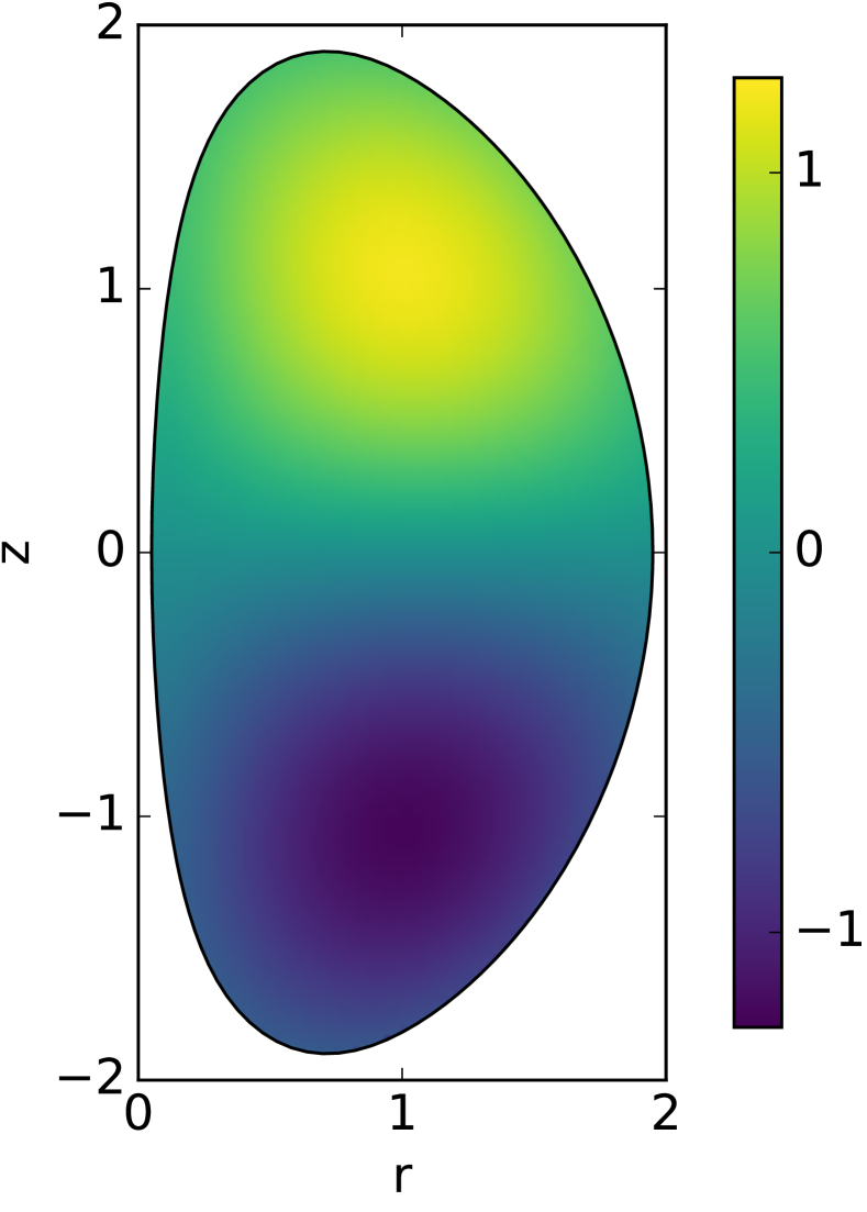
(a) The radial component, $B_{r}$.

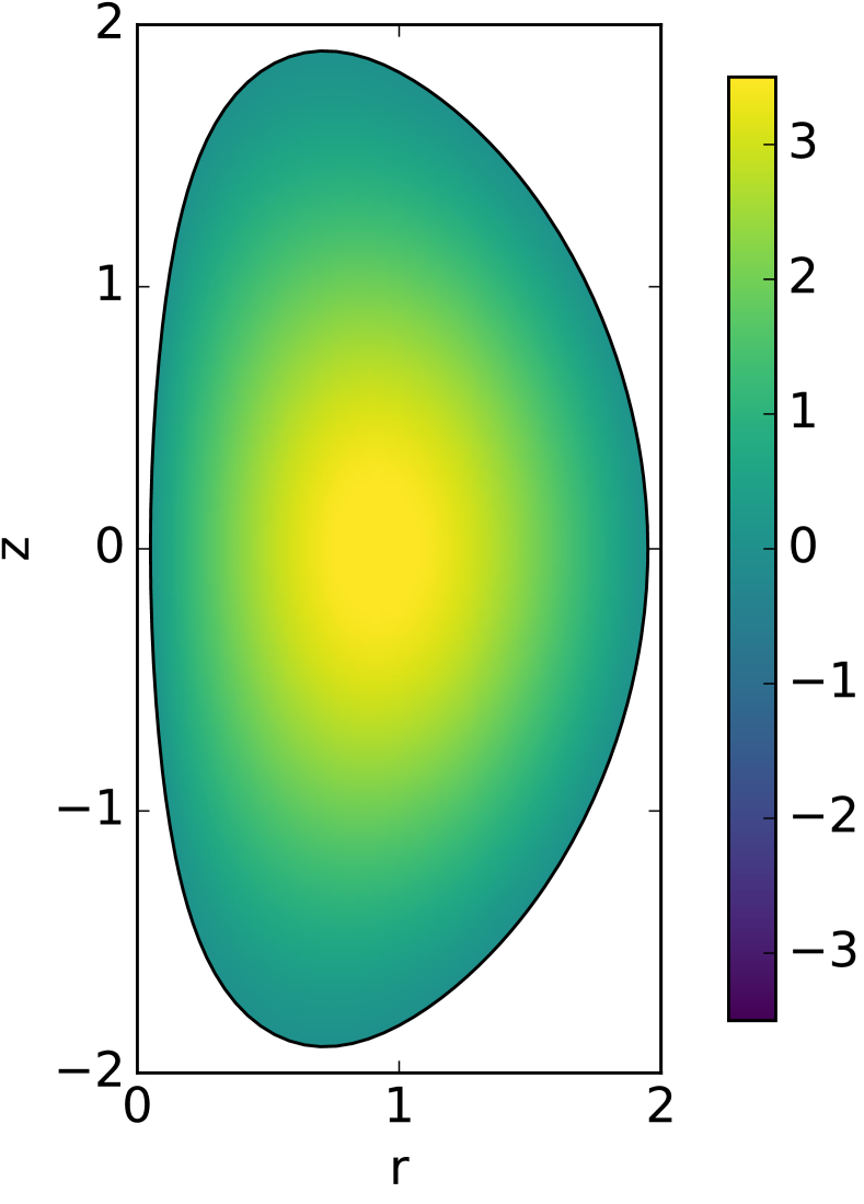
(b) The azimuthal component, $B_{\phi}$.

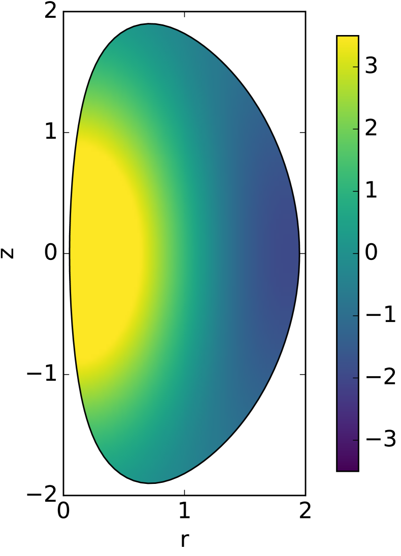
(c) The $z$ component, $B_{z}$.

Figure 4: The Beltrami field $\bm{B}$ in the $\phi=0$ plane.

Treating $\lambda$ and $c_{1},\ldots,c_{6}$ as unknowns, we solve for these values by imposing seven boundary conditions on $\psi$ chosen such that the boundary of the plasma, given by the implicit equation $\psi=0$, best approximates the parametric curve

$$r(t) =1+\epsilon\cos\left(t+\alpha\sin t\right)$$ (6.4)

$$z(t) =\epsilon\kappa\sin t,$$

with $t\in[0,2\pi)$. This curve describes a wide class of experimentally relevant axisymmetric plasma boundaries [45], where $\epsilon$ is the inverse aspect ratio, $\kappa$ is the elongation, and $\sin\alpha=\delta$ is the triangularity. The boundary conditions enforced on $\psi$ are [13]

$$\psi(1+\epsilon,0,\bm{c}) =0,$$ (6.5)

$$\psi(1-\epsilon,0,\bm{c}) =0,$$

$$\psi(1-\delta\epsilon,-\kappa\epsilon,\bm{c}) =0,$$

$$\psi_{r}(1-\delta\epsilon,-\kappa\epsilon,\bm{c}) =0,$$

$$\psi_{zz}(1+\epsilon,0,\bm{c})+N_{1}\psi_{r}(1+\epsilon,0,\bm{c}) =0,$$

$$\psi_{zz}(1-\epsilon,0,\bm{c})+N_{2}\psi_{r}(1-\epsilon,0,\bm{c}) =0,$$

$$\psi_{rr}(1-\delta\epsilon,-\kappa\epsilon,\bm{c})+N_{3}\psi_{z}(1-\delta\epsilon,-\kappa\epsilon,\bm{c}) =0,$$

where the subscripts refer to partial derivatives with respect to the specified variable, the vector of parameters is $\bm{c}=(c_{1},\cdots,c_{6},\lambda)$, and $N_{1}$, $N_{2}$ and $N_{3}$ are the curvatures at the outer equatorial point, the inner equatorial point, and the top point, respectively, given by the formulae

$$N_{1}=-\frac{(1+\alpha)^{2}}{\epsilon\kappa^{2}},\qquad N_{2}=\frac{(1-\alpha)^{2}}{\epsilon\kappa^{2}},\qquad N_{3}=\frac{\kappa}{\epsilon\cos^{2}\alpha}.$$ (6.6)

Equation (6.5) is a non-linear system of 7 equations for 7 unknowns. Given reasonable initial conditions, it can be solved without difficulty using standard non-linear root finding packages.

Table 1: Convergence data for Example 1: A genus one Taylor state. Relative errors are reported in the field $\bm{B}$ at the point $r=1.2$, $\phi=0$, $z=0.25$. The reference field $\bm{B}_{\text{exact}}$ is calculated using $\psi$ from (6.1).

$n$	$\operatorname{Re}B_{r}$	$\operatorname{Re}B_{\phi}$	$\operatorname{Re}B_{z}$	$|\bm{B}-\bm{B}_{\text{exact}}|/|\bm{B}_{\text{exact}}|$
25	0.443052524078644	3.10056763474524	-3.784408049008867E-002	$2.7\cdot 10^{-3}$
50	0.442014263551259	3.09845144534915	-4.109405171821609E-002	$2.5\cdot 10^{-5}$
100	0.442018001760211	3.09850436011175	-4.104126312770094E-002	$3.9\cdot 10^{-8}$
200	0.442017994270342	3.09850428092008	-4.104130814605825E-002	$1.2\cdot 10^{-8}$

We achieve near machine precision residual using Matlab’s fsolve function. Once $\bm{c}$ has been determined, the Taylor state is completely defined. Using the fact that $\nabla\times\bm{B}=\lambda\bm{B}$, and relation (6.1), we can numerically evaluate the toroidal flux as

$$\Phi^{\text{tor}} =\int_{S_{t}}\bm{B}\cdot d\bm{a}$$ (6.7)

$$=\frac{1}{\lambda}\int_{\gamma}\bm{B}\cdot d\bm{l}$$

$$=\frac{1}{\lambda}\int_{\gamma}\frac{1}{r}\left(\nabla\psi\times\bm{\phi}\right)\cdot d\bm{l}.$$

This integral can be computed to spectral accuracy using the trapezoidal rule. The integral equation-based Beltrami solver of this paper can be tested against this exact Taylor state by solving the problem

$$\nabla\times\bm{B} =\lambda\bm{B} \text{in }\Omega,$$ (6.8)

$$\bm{B}\cdot\bm{\mathsf{n}} =0 \text{on }\Gamma,$$

$$\int_{S_{t}}\bm{B}\cdot d\bm{a} =\Phi^{\text{tor}}.$$

To highlight the robustness and accuracy of our solver, we choose equilibrium parameters that are particularly challenging from a numerical point of view: very low aspect ratio, $\epsilon=0.95$, moderate triangularity, $\delta=0.3$, and high elongation, $\kappa=2$. See Figure 4 for a plot of the real part of $\bm{B}$, and Table 1 for convergence data. We report the relative $\ell^{2}$-error at the arbitrary point $(r,\phi,z)=(1.2,0,0.25)$ for various values of $n$, the number of points used in discretizing the geometry. Observe that in our method, the interior of $\Omega$ is not discretized, and we are free to evaluate the field at any point of the domain. We chose $(1.2,0,0.25)$ because the error at this point is representative of the error at any other point inside $\Omega$. The solver converges rapidly to a precision of roughly $10^{-8}$. This precision is most likely due to a combination of the accuracy to which we evaluated the modal-Green’s functions – set to be an absolute precision of $10^{-12}$ inside the adaptive Gaussian quadrature routine – and the conditioning of the system matrix – $\kappa(\bm{\mathsf{A}})\sim 10^{4}$ incurred by spectral differentiation. Increased precision could be obtained by more accurate evaluation of the modal Green’s functions, and constructing the approximation to $\Delta_{\Gamma}^{-1}$ using an integral method instead of inverting a spectral differentiation matrix. These minor numerical improvements are discussed more thoroughly in [26].

6.2 Example 2: Axisymmetric Taylor state within a toroidal shell with very low aspect ratio

The previous equilibrium can also be used to verify the accuracy and performance of our solver for Taylor states in toroidal shells. The flux surface $\psi=0.5$ can be taken as the inside surface, $\Gamma^{\text{in}}$, and the surface $\psi=0$ can be taken as the outside surface, $\Gamma^{\text{out}}$. The toroidal shell is then bounded by $\Gamma^{\text{in}}$ and $\Gamma^{\text{out}}$. Let $S_{t}$ be the spanning surface obtained from the intersection of $\Omega$ with the plane $\phi=0$. In this case, the toroidal flux is given as

$$\Phi^{\text{tor}}=\frac{1}{\lambda}\left(\int_{\gamma_{\text{out}}}\frac{1}{r}\left(\nabla\psi\times\bm{\phi}\right)\cdot d\bm{l}-\int_{\gamma_{\text{in}}}\frac{1}{r}\left(\nabla\psi\times\bm{\phi}\right)\cdot d\bm{l}\right),$$ (6.9)

where $\gamma_{\text{out}}$ and $\gamma_{\text{in}}$ are the generating curves for $\Gamma^{\text{out}}$ and $\Gamma^{\text{in}}$, respectively. Furthermore, by definition of the flux function $\psi$ [14], the poloidal flux is given by the simple formula:

$$\Phi^{\text{pol}} =2\pi\left(\psi(r_{\text{out}},0)-\psi(r_{\text{in}},0)\right)$$ (6.10)

$$=2\pi\left(0-0.5\right)$$

$$=-\pi$$

The values $r_{\text{out}}$ and $r_{\text{in}}$ are the radial coordinates corresponding to $\psi=0$ and $\psi=0.5$ for $z=0$, respectively. With these conditions, the magnetic field $\bm{B}$ is given by (6.1), with $\psi$ given by (6.3), and the constants $c_{1},\ldots,c_{6}$, and $\lambda$ determined by solving the system (6.5).

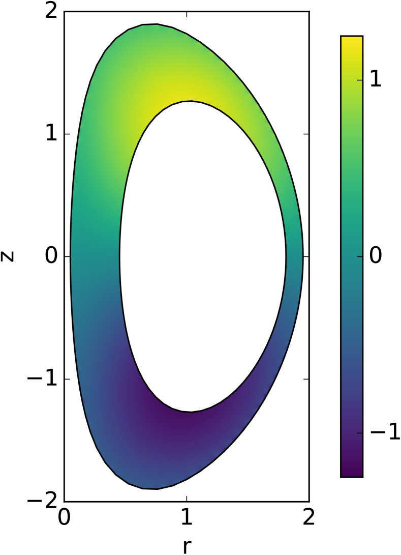
(a) The radial component, $B_{r}$.

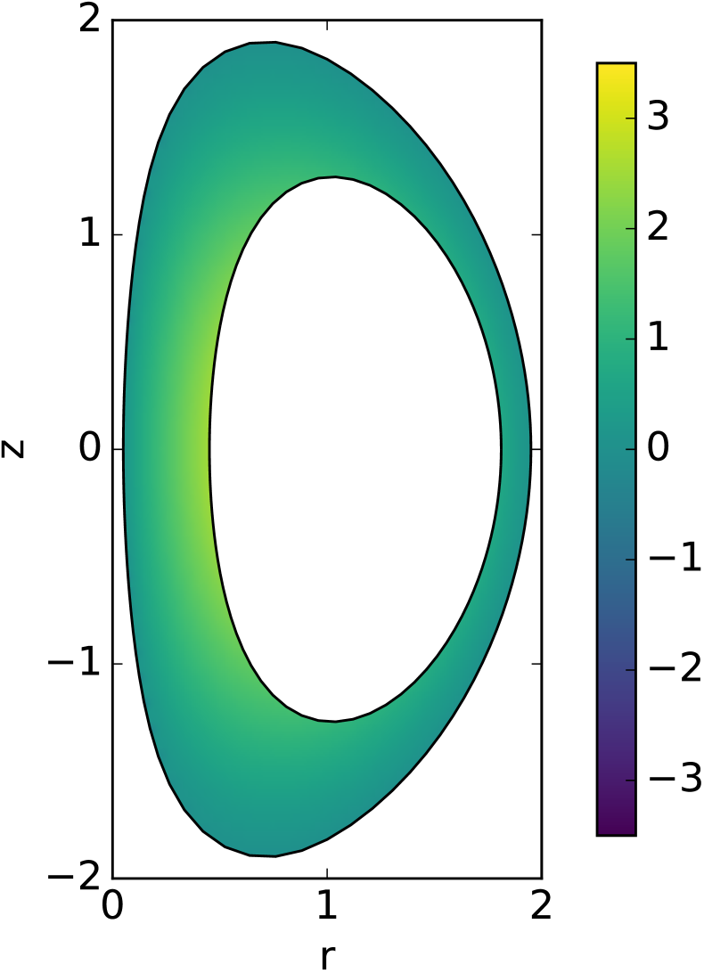
(b) The azimuthal component, $B_{\phi}$.

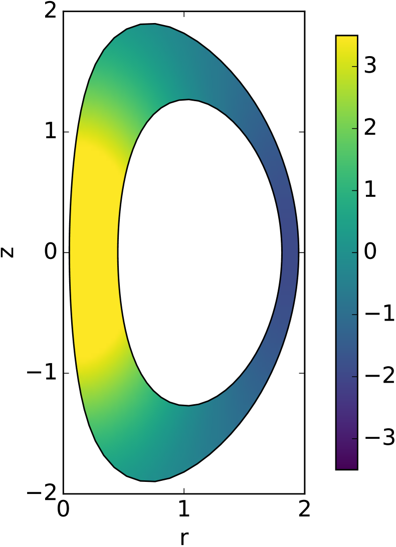
(c) The $z$ component, $B_{z}$.

Figure 5: The Beltrami field $\bm{B}$ in the $\phi=0$ plane bounded by the surfaces $\psi=0.5$ and $\psi=0$.

See Figure 5 for a plot of the real part of $\bm{B}$ in the toroidal shell, and Table 2 for convergence data. It is worth noting that the field $\bm{B}$ in the genus two shell is exactly the same $\bm{B}$ as in the genus one torus. The additional boundary was merely calculated from the flux function $\psi$. However, the integral equation solver has no knowledge of this, and is able to reproduce exactly the same field. As before, we report the relative $\ell^{2}$-error at the point $(r,\phi,z)=(1.2,0,0.25)$ for various values of $n$, the number of points used in discretizing the geometry. We observe once more that our solver converges to a very accurate solution with few points on the boundary.

Table 2: Convergence data for Example 2: A genus two Taylor state. Relative errors are reported in the field $\bm{B}$ at the point $r=0.5$, $\phi=0$, $z=-1.5$. The reference field $\bm{B}_{\text{exact}}$ is calculated using $\psi$ from (6.1).

$n$	$\operatorname{Re}B_{r}$	$\operatorname{Re}B_{\phi}$	$\operatorname{Re}B_{z}$	$|\bm{B}-\bm{B}_{\text{exact}}|/|\bm{B}_{\text{exact}}|$
25	-0.7790590773628590	0.5058371725845370	0.9957374643442100	$1.3\cdot 10^{-2}$
50	-0.7758504363890280	0.5043487336557070	0.9869834030024680	$7.3\cdot 10^{-4}$
100	-0.7754614741802320	0.5046765566326400	0.9867586238268730	$3.0\cdot 10^{-6}$
200	-0.7754611961412940	0.5046760189196530	0.9867575110491060	$8.6\cdot 10^{-7}$

6.3 Example 3: Non-axisymmetric Taylor state

Solutions to the boundary value problem (1.3) are not always purely axisymmetric. Only purely axisymmetric solutions contribute to the toroidal and poloidal fluxes, but non-trivial, zero-flux Beltrami fields also exist [55]. We focus here on the genus-1 toroidal case for simplicity, as the genus-2 case is identical. Let $\lambda$ be an eigenvalue for the boundary value problem corresponding to the $l^{\text{th}}$-Fourier mode solution. That is to say, let $\lambda$ be such that there exists a non-trivial solution to the problem:

$$\nabla\times\bm{B}_{\ell} =\lambda\bm{B}_{\ell} \text{in }\Omega,$$ (6.11)

$$\bm{B}_{\ell}\cdot\bm{\mathsf{n}} =0 \text{on }\Gamma,$$

where $\bm{B}_{\ell}=\bm{B}_{\ell}(r,z)\,e^{i\ell\phi}$.

Using the method of [61, 8], roots of the Fredholm determinant of the Beltrami integral equation (3.7) can be found as a function of the Beltrami parameter $\lambda$. These roots correspond exactly to eigenvalues of the Beltrami boundary-value problem. The eigenvalues for the $\ell=1$ mode located on the interval $[1.0,8.0]$ are reported in Table 3, along with absolute errors estimated as in [61]. These values were obtained from discretizing the $\ell=1$ Fourier mode, in a way analogous to the azimuthal mode $\ell=0$ as described in Section 5, using $n=100$ points on the boundary of the shape given by the following parameterization

$$r(t) =2+\epsilon\cos\left(t+\alpha\sin t\right)$$ (6.12)

$$z(t) =\epsilon\kappa\sin t,$$

for $t\in[0,2\pi)$ with $\epsilon=0.85$, $\sin\alpha=0.3$, and $\kappa=2.0$. The errors reported in Table 3 are generally commensurate with the smallest singular value of the discretized system.

Table 3: Beltrami eigenvalues for the $\ell=1$ Fourier mode on the interval $[1,8]$.

$\lambda$	Error
2.81618429764383	$2.3\cdot 10^{-7}$
3.22821787079846	$3.3\cdot 10^{-7}$
4.01342328856135	$5.8\cdot 10^{-9}$
4.45732687692555	$1.0\cdot 10^{-8}$
4.75909602398894	$1.3\cdot 10^{-8}$
4.80160935115718	$8.9\cdot 10^{-9}$
5.52819229381708	$1.0\cdot 10^{-10}$
5.56546068190407	$5.8\cdot 10^{-10}$
6.13551340937516	$6.4\cdot 10^{-12}$
6.34490415618171	$1.4\cdot 10^{-11}$
6.55792492108800	$8.2\cdot 10^{-12}$
6.63664744243683	$1.1\cdot 10^{-11}$
7.07387937977634	$4.8\cdot 10^{-12}$
7.14679867372582	$5.0\cdot 10^{-12}$
7.44941373173176	$1.0\cdot 10^{-11}$
7.81008353287565	$6.6\cdot 10^{-12}$
7.88508920256358	$2.9\cdot 10^{-11}$

Empirically, as shown via a numerical calculation of the singular values of the discretized matrix, the eigenspace corresponding to each of the eigenvalues in Table 3 is one-dimensional. The eigenvector (i.e. the corresponding generalized Debye source) can be computed by using the method of [53]. That is, we take a random vector $\bm{\mathsf{r}}$ and apply the discretized system matrix $\bm{\mathsf{A}}$ to it to compute $\bm{\mathsf{y}}=\bm{\mathsf{A}}\bm{\mathsf{r}}.$ Next, using standard Gaussian elimination, we solve the system $\left(\bm{\mathsf{A}}+\bm{\mathsf{r}}_{1}\bm{\mathsf{r}}^{T}_{2}\right)\bm{\mathsf{x}}=\bm{\mathsf{y}}$, with $\bm{\mathsf{r}}_{1}$ and $\bm{\mathsf{r}}_{2}$ random vectors. The matrix $\bm{\mathsf{A}}+\bm{\mathsf{r}}_{1}\bm{\mathsf{r}}^{T}_{2}$ is uniquely invertible with probability one if $\bm{\mathsf{A}}$ is exactly rank-one deficient, as in our case. Since $\bm{\mathsf{y}}$ is in the range of $\bm{\mathsf{A}}$, we have that $\bm{\mathsf{A}}\bm{\mathsf{x}}=\bm{\mathsf{y}}$, and therefore $\bm{\mathsf{z}}=\bm{\mathsf{x}}-\bm{\mathsf{r}}$ is a null-vector of $\bm{\mathsf{A}}$. We then normalize $\bm{\mathsf{z}}$, which represents a discretization of $\sigma$, the generalized Debye source, so that $\int_{\gamma}|\sigma|^{2}ds=1$. Components of the zero-flux Beltrami fields for the first five $\lambda$’s greater than give are show in Figure 6.

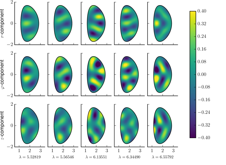
Figure 6: Slices of non-axisymmetric, zero-flux Beltrami fields in the $\phi=0$ plane corresponding to the first five resonances larger than 5 with azimuthal dependence of $e^{i\phi}$. The modal Debye sources were normalized to have unit norm along the generating curve, $\int_{\gamma}|\sigma_{1}|^{2}ds=1$.

7 Conclusions

We have presented a numerical algorithm for the calculation of Beltrami (force-free) fields in the interior of toroidally axisymmetric geometries, both genus one and two, and given explicit numerical examples demonstrating the accuracy of the solver. The representation of Beltrami fields is based on earlier work regarding the representation of Maxwell fields in the context of scattering phenomena. It ensures that (by construction) the resulting field is a Beltrami field, and leads directly to a second-kind integral equation which can be numerically inverted to high precision. Moreover, the solver has low memory requirements since the unknowns in the integral equation are defined on the boundary of the domain; the interior of the domain does not need to be discretized. The solver can be used to study toroidally axisymmetric Taylor states in laboratory, space, and astrophysical plasmas, as well as bifurcations to the fully three-dimensional, non-axisymmetric states corresponding to resonances of the Beltrami parameter $\lambda$.

Our formulation extends directly to non-axisymmetric domains, as required for stellarator equilibrium calculations for example [40]. In that context, the results presented here are promising, since high accuracy is reached with a modest number of unknowns, even for low aspect ratio, highly elongated domains. This, along with the low memory requirements, are desirable features for computations of three-dimensional MHD equilibria which rely on the iterative calculation of multiple Taylor states in genus-one and genus-two regions [40]. The fact that the interior of the domain is not discretized in our scheme and that none of the quantities need to be evaluated in the interior is particularly attractive for that application, since the force balance conditions between adjacent Taylor states only need to be evaluated at the ideal MHD interfaces at each iteration. The entire iterative procedure could thus be implemented by discretizing the ideal MHD surfaces only, and the magnetic field would only be evaluated in the entire domain at the very end, once global force balance has been reached. This would lead to significant savings in run-time and in memory, and motivates detailed code-to-code comparisons with the scheme used in SPEC [40] to identify the strengths and weaknesses of each approach. However, for our numerical solver to be applicable to general three dimensional toroidal domains, details in the numerical implementation need to be modified. Specifically, we are currently working on addressing questions regarding the discretization of the domain, the evaluation of differential surface operators, and the computation of numerical quadratures.

Furthermore, regarding code-to-code comparisons, one thing seems clear at this stage: the scheme of this work is the only one in which only the boundary is discretized. This leads to a major reduction in the number of unknowns as compared to other existing schemes, as we have highlighted on several occasions throughout the paper.

Lastly, with minor changes the representation and algorithm described are applicable in exterior, unbounded geometries (both simply- and multiply-connected). We have, however, left this discussion out of this article because of the present focus on plasma physics applications.

References

- [1] B. Alpert. Hybrid Gauss-trapezoidal quadrature rules. SIAM J. Sci. Comput., 20(5):1551–1584, 1999.
- [2] T. Amari, J. J. Aly, J. F. Luciani, T. Z. Boulmezaoud, and Z. Mikic. Reconstructing the Solar Coronal Magnetic Field as a Force-Free Magnetic Field. Solar Physics, 174(1):129–149, 1997.
- [3] T. Amari, C. Boulbe, and T. Z. Boulmezaoud. Computing Beltrami Fields. SIAM J. Sci. Comput., 31(5):3217 – 3254, 2009.
- [4] E. Anderson, Z. Bai, C. Bischof, S. Blackford, J. Demmel, J. Dongarra, J. Du Croz, A. Greenbaum, S. Hammarling, A. McKenney, and D. Sorensen. LAPACK Users’ Guide. Society for Industrial and Applied Mathematics, Philadelphia, PA, third edition, 1999.
- [5] D. J. Battaglia, M. W. Bongard, R. J. Fonck, A. J. Redd, and A. C. Sontag. Tokamak Startup Using Point-Source dc Helicity Injection. Phys. Rev. Lett., 102:225003, 2009.
- [6] P. M. Bellan. Fundamentals of Plasma Physics. Cambridge University Press, 2006.
- [7] T. Z. Boulmezaoud and T. Amari. Approximation of linear force-free fields in bounded 3-D domains. Math. Comput. Model., 31:109–129, 2000.
- [8] J. P. Boyd. Computing zeros on a real interval through Chebyshev expansion and polynomial rootfinding. SIAM J. Numer. Anal., 40:1666–1682, 2002.
- [9] J. Bremer. On the Nyström discretization of integral equations on planar curves with corners. Appl. Comput. Harm. Anal., 32:45–64, 2012.
- [10] J. Bremer, V. Rokhlin, and I. Sammis. Universal quadratures for boundary integral equations on two-dimensional domains with corners. J. Comput. Phys., 229:8259–8280, 2010.
- [11] O. P. Bruno and P. Laurence. Existence of three-dimensional toroidal MHD equilibria with nonconstant pressure. Comm. Pure Appl. Math., 49(7):717–764, 1996.
- [12] B. C. Carlson. Computing elliptic integrals by duplication. Numer. Math., 33:1–16, 1979.
- [13] A. J. Cerfon and J. P. Freidberg. “One size fits all" analytic solutions to the Grad-Shafranov equation. Phys. Plasmas, 17:032502, 2010.
- [14] A. J. Cerfon and M. O’Neil. Exact axisymmetric taylor states for shaped plasmas. Phys. Plasmas, 21:064501, 2014.
- [15] S. Chandrasekhar. On force-free magnetic fields. Proc. Natl. Acad. Sci., 42(1):1, 1956.
- [16] E. V. Chernokozhin and A. Boag. Method of generalized debye sources for the analysis of electromagnetic scattering by arbitrary shaped bodies. In 2012 6th European Conference on Antennas and Propagation (EUCAP), pages 3219–3221, March 2012.
- [17] H. S. Cohl and J. E. Tohline. A Compact Cylindrical Green’s Function Expansion for the Solution of Potential Problems. Astrophys. J., 527:86–101, 1999.
- [18] D. Colton and R. Kress. Integral Equation Methods in Scattering Theory. John Wiley & Sons, Inc., 1983.
- [19] P. Constantin and A. Majda. The Beltrami Spectrum for Incompressible Fluid Flows. Commun. Math. Phys., 115:435–456, 1988.
- [20] J. T. Conway and H. S. Cohl. Exact Fourier expansion in cylindrical coordinates for the three-dimensional Helmholtz Green function. Z. Angew. Math. Phys., 61:425–442, 2010.
- [21] C. D. Cothran, M. R. Brown, T. Gray, M. J. Schaffer, and G. Marklin. Observation of a Helical Self-Organized State in a Compact Toroidal Plasma. Phys. Rev. Lett., 103:215002, 2009.
- [22] G. R. Dennis, S. R. Hudson, D. Terranova, P. Franz, R. L. Dewar, and M. J. Hole. Minimally Constrained Model of Self-Organized Helical States in Reversed-Field Pinches. Phys. Rev. Lett., 111:055003, 2013.
- [23] C. L. Epstein and L. Greengard. Debye sources and the numerical solution of the time harmonic Maxwell equations. Comm. Pure Appl. Math., 63(4):413–463, 2010.
- [24] C. L. Epstein, L. Greengard, and M. O’Neil. Debye sources and the numerical solution of the time harmonic Maxwell equations II. Comm. Pure Appl. Math., 66(5):753–789, 2013.
- [25] C. L. Epstein, L. Greengard, and M. O’Neil. Debye Sources, Beltrami Fields, and a Complex Structure on Maxwell Fields. Comm. Pure Appl. Math., 68(12):2237–2280, 2016.
- [26] C. L. Epstein, L. Greengard, and M. O’Neil. A high-order wideband direct solver for electromagnetic scattering from bodies of revolution. 2017. arXiv:1708.00056 [math.NA].
- [27] N. Flyer, B. Fornberg, S. Thomas, and B. C. Low. Magnetic Field Confinement in the Solar Corona. I. Force-Free Magnetic Fields. Astrophys. J., 606:1210 – 1222, 2004.
- [28] T. Frankel. The Geometry of Physics. Cambridge University Press, Cambridge, UK, 3rd edition, 2011.
- [29] C. G. R. Geddes, T. W. Kornack, and M. R. Brown. Scaling studies of spheromak formation and equilibrium. Phys. Plasmas, 5:1027, 1998.
- [30] A. Gil, J. Segura, and N. M. Temme. Numerical Methods for Special Functions. SIAM, Philadelphia, PA, 2007.
- [31] C. Gimblett, R. Hastie, and P. Helander. The role of edge current-driven modes in elm activity. Plasma physics and controlled fusion, 48(10):1531, 2006.
- [32] H. Grad and H. Rubin. Hydromagnetic equilibria and force-free fields. Proceedings of the Second United Nations Conference on the Peaceful Uses of Atomic Energy, 31:190, 1958.
- [33] S. Hao, A. H. Barnett, P.-G. Martinsson, and P. Young. High-order accurate Nystrom discretization of integral equations with weakly singular kernels on smooth curves in the plane. Adv. Comput. Math., 40:245–272, 2014.
- [34] R. Hastie. The Taylor relaxed state in tokamaks and the sawtooth collapse. Nuclear Fusion, 29(1):96, 1989.
- [35] J. Helsing and A. Karlsson. An explicit kernel-split panel-based Nyström scheme for integral equations on axially symmetric surfaces. J. Comput. Phys., 272:686–703, 2014.
- [36] J. Helsing and A. Karlsson. Determination of normalized magnetic eigenfields in microwave cavities. IEEE Trans. Microw. Theory Tech., 63:1457–1467, 2015.
- [37] J. Helsing and A. Karlsson. Determination of normalized electric eigenfields in microwave cavities with sharp edges. J. Comput. Phys., 304:465–486, 2016.
- [38] J. Helsing and R. Ojala. Corner singularities for elliptic problems: Integral equations, graded meshes, quadrature, and compressed inverse preconditioning. J. Comput. Phys., 227(20):8820–8840, 2008.
- [39] R. Hiptmair, P. R. Kotiuga, and S. Tordeux. Self-adjoint curl operators. Ann. Mat. Pura Appl., 191(3):431–457, 2012.
- [40] S. R. Hudson, R. L. Dewar, G. Dennis, M. J. Hole, M. McGann, G. von Nessi, and S. Lazerson. Computation of multi-region relaxed magnetohydrodynamics equilibria. Phys. Plasmas, 19:112502, 2012.
- [41] S. R. Hudson, R. L. Dewar, M. J. Hole, and M. McGann. Non-axisymmetric, multi-region relaxed magnetohydrodynamic equilibrium solutions. Plasma Phys. Control. Fusion, 54:014005, 2012.
- [42] R. Kress. On an exterior boundary-value problem for the time-harmonic Maxwell equations with boundary conditions for the normal components of the electric and magnetic field. Math. Meth. Appl. Sci., 8(1):77–92, 1986.
- [43] R. Kress. On constant-alpha force-free fields in a torus. J. Engrg. Math., 20(4):323–344, 1986.
- [44] L. L. Lao, H. S. John, R. D. Stambaugh, A. G. Kellman, and W. Pfeiffer. Reconstruction of Current Profile Parameters and Plasma Shapes in Tokamaks. Nuclear Fusion, 25(11):1611, 1985.
- [45] R. L. Miller, M. S. Chu, J. M. Greene, Y. R. Lin-Liu, and R. E. Waltz. Noncircular, finite aspect ratio, local equilibrium model. Phys. Plasmas, 5:973, 1998.
- [46] J.-C. Nédélec. Acoustic and electromagnetic equations. Springer, New York, NY, 1988.
- [47] F. W. Olver, D. W. Lozier, R. F. Boisvert, and C. W. Clark. NIST Handbook of Mathematical Functions. Cambridge University Press, New York, NY, USA, 1st edition, 2010.
- [48] A. Pataki, A. J. Cerfon, J. P. Freidberg, L. Greengard, and M. O’Neil. A fast, high-order solver for the Grad-Shafranov equation. J. Comput. Phys, 243:28–45, 2013.
- [49] R. Picard. On a selfadjoint realization of curl in exterior domains. Math. Z., 229:319–338, 1998.
- [50] H. Qin, W. Liu, H. Li, and J. Squire. Woltjer-Taylor State without Taylor’s Conjecture: Plasma Relaxation at all Wavelengths. Phys. Rev. Lett., 109:235001, 2012.
- [51] A. K. Ram, B. Dasgupta, V. Krishnamurthy, and D. Mitra. Anomalous Diffusion of Field Lines and Charged Particles in Arnold-Beltrami-Childress Force-Free Magnetic Fields. Phys. Plasmas, 21:072309, 2014.
- [52] V. Shafranov. On magnetohydrodynamical cquilibrium configurations. Soviet Physics – JETP, 6:545, 1958.
- [53] J. Sifuentes, Z. Gimbutas, and L. Greengard. Randomized methods for rank-deficient linear systems. Elec. Trans. Num. Anal., 44:177–188, 2015.
- [54] X. Z. Tang and A. H. Boozer. Chandrasekhar-Kendall Modes and Taylor Relaxation in an Axisymmetric torus. Phys. Plasmas, 12:102102, 2005.
- [55] J. B. Taylor. Relaxation and magnetic reconnection in plasmas. Reviews of Modern Physics, 58(3):741, 1986.
- [56] J. B. Taylor. Relaxation revisited. Phys. Plasmas, 7:1623, 2000.
- [57] L. N. Trefethen. Spectral Methods in MATLAB. SIAM, Philadelphia, PA, 2000.
- [58] P. Werner. On an integral equation in electromagnetic diffraction theory. J. Math. Anal. Appl., 14:445–462, 1966.
- [59] L. Woltjer. A theorem on force-free magnetic fields. Proc. Natl. Acad. Sci., 44(6):489, 1958.
- [60] P. Young, S. Hao, and P.-G. Martinsson. A high-order Nyström discretization scheme for boundary integral equations defined on rotationally symmetric surfaces. J. Comput. Phys., 231(11):4142–4159, 2012.
- [61] L. Zhao and A. Barnett. Robust and efficient solution of the drum problem via Nyström approximation of the Fredholm determinant . SIAM J. Numer. Anal., 53:1984–2007, 2015.