A Formal Approach to Cyber-Physical Attacks

Abstract

We apply formal methods to lay and streamline theoretical foundations to reason about Cyber-Physical Systems (CPSs) and cyber-physical attacks. We focus on integrity and DoS attacks to sensors and actuators of CPSs, and on the timing aspects of these attacks. Our contributions are threefold: (1) we define a hybrid process calculus to model both CPSs and cyber-physical attacks; (2) we define a threat model of cyber-physical attacks and provide the means to assess attack tolerance/vulnerability with respect to a given attack; (3) we formalise how to estimate the impact of a successful attack on a CPS and investigate possible quantifications of the success chances of an attack. We illustrate definitions and results by means of a non-trivial engineering application.

I Introduction

Context and motivation

Cyber-Physical Systems (CPSs) are integrations of networking and distributed computing systems with physical processes that monitor and control entities in a physical environment, with feedback loops where physical processes affect computations and vice versa. For example, in real-time control systems, a hierarchy of sensors, actuators and control processing components are connected to control stations. Different kinds of CPSs include supervisory control and data acquisition (SCADA), programmable logic controllers (PLC) and distributed control systems.

In recent years there has been a dramatic increase in the number of attacks to the security of cyber-physical and critical systems, e.g., manipulating sensor readings and, in general, influencing physical processes to bring the system into a state desired by the attacker. Many (in)famous examples have been so impressive to make the international news, e.g.: the Stuxnet worm, which reprogrammed PLCs of nuclear centrifuges in Iran [5] or the attack on a sewage treatment facility in Queensland, Australia, which manipulated the SCADA system to release raw sewage into local rivers and parks [18].

As stated in [8], the concern for consequences at the physical level puts CPS security apart from standard information security, and demands for ad hoc solutions to properly address such novel research challenges. The works that have taken up these challenges range from proposals of different notions of cyber-physical security and attacks (e.g., [3, 8, 11], to name a few) to pioneering extensions to CPS security of standard formal approaches (e.g., [3, 4, 22]). However, to the best of our knowledge, a systematic formal approach to cyber-physical attacks is still to be fully developed.

Background

The dynamic behaviour of the physical plant of a CPS is often represented by means of a discrete-time state-space model consisting of two equations of the form

$$\begin{array}[]{rcl}x_{k+1}=Ax_{k}+Bu_{k}+w_{k}&\mathrm{and}&y_{k}=Cx_{k}+e_{k}\,,\end{array}$$

where $x_{k}\in\mathbb{R}^{n}$ is the current (physical) state, $u_{k}\in\mathbb{R}^{m}$ is the input (i.e., the control actions implemented through actuators) and $y_{k}\in\mathbb{R}^{p}$ is the output (i.e., the measurements from the sensors). The uncertainty $w_{k}\in\mathbb{R}^{n}$ and the measurement error $e_{k}\in\mathbb{R}^{p}$ represent perturbation and sensor noise, respectively, and $A$, $B$, and $C$ are matrices modelling the dynamics of the physical system. Here, the next state $x_{k+1}$ depends on the current state $x_{k}$ and the corresponding control actions $u_{k}$, at the sampling instant $k\in\mathbb{N}$. The state $x_{k}$ cannot be directly observed: only its measurements $y_{k}$ can be observed.

The physical plant is supported by a communication network through which the sensor measurements and actuator data are exchanged with controller(s) and supervisor(s) (e.g., IDSs), which are the cyber components (also called logics) of a CPS.

Contributions

In this paper, we focus on a formal treatment of both integrity and Denial of Service (DoS) attacks to physical devices (sensors and actuators) of CPSs, paying particular attention to the timing aspects of these attacks. The overall goal of the paper is to apply formal methodologies to lay theoretical foundations to reason about and statically detect attacks to physical devices of CPSs.

Our contributions are threefold. The first contribution is the definition of a hybrid process calculus, called CCPSA, to formally specify both CPSs and cyber-physical attacks. In CCPSA, CPSs have two components: a physical component denoting the physical plant (also called environment) of the system, and containing information on state variables, actuators, sensors, evolution law, etc., and a cyber component that governs access to sensors and actuators, channel-based communication with other cyber components. Thus, channels are used for logical interactions between cyber components, whereas sensors and actuators make possible the interaction between cyber and physical components.

CCPSA adopts a discrete notion of time [9] and it is equipped with a labelled transition semantics (LTS) that allows us to observe both physical events (system deadlock and violations of safety conditions) and cyber events (channel communications). Based on our LTS, we define two trace-based system preorders: a trace preorder, $\sqsubseteq$, and a timed variant, $\sqsubseteq_{m..n}$, for $m,n\in\mathbb{N}^{+}\cup\infty$, which takes into account discrepancies of execution traces within the time interval $m..n$.

As a second contribution, we formalise a threat model that specifies attacks that can manipulate sensor and/or actuator signals in order to drive a CPS into an undesired state [19]. Cyber-physical attacks typically tamper with both the physical (sensors and actuators) and the cyber layer. In our threat model, communication cannot be manipulated by the attacker, who instead may compromise (unsecured) physical devices, which is our focus. As depicted in Figure 1, our attacks may affect directly the sensor measurements or the controller commands.

• Attacks on sensors consist of reading and eventually replacing $y_{k}$ (the sensor measurements) with $y^{a}_{k}$.

• Attacks on actuators consist of reading, eavesdropping and eventually replacing the controller commands $u_{k}$ with $u^{a}_{k}$, affecting directly the actions the actuators may execute.

We group attacks into classes. A class of attacks takes into account both the malicious activity $\mathcal{I}$ on physical devices and the timing parameters $m$ and $n$ of the attack: begin and end of the attack. We represent a class $C$ as a total function $C\in[\mathcal{I}\rightarrow{\cal P}(m..n)]$. Intuitively, for $\iota\in\mathcal{I}$, $C(\iota)\subseteq m..n$ denotes the set of time instants when an attack of class $C$ may tamper with the device $\iota$. As observed in [11], timing is a critical issue in CPSs because the physical state of a system changes continuously over time, and as the system evolves in time, some states might be more vulnerable to attacks than others. For example, an attack launched when the target state variable reaches a local maximum (or minimum) may have a great impact on the whole system behaviour [12]. Furthermore, not only the timing of the attack but also the duration of the attack is an important parameter to be taken into consideration in order to achieve a successful attack. For example, it may take minutes for a chemical reactor to rupture [20], hours to heat a tank of water or burn out a motor, and days to destroy centrifuges [5].

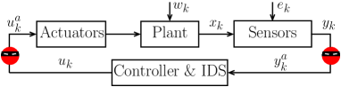
Figure 1: Our threat model for CPSs

In order to make security assessments on our CPSs, we adopt a well-known approach called Generalized Non Deducibility on Composition (GNDC) [6]. Thus, in CCPSA, we say that a CPS $\mathit{Sys}$ tolerates a cyber-physical attack $A$ if

$$\mathit{Sys}\>\parallel\>A\>\;\sqsubseteq\>\;\mathit{Sys}\enspace.$$

In this case, the presence of the attack $A$, does not affect the whole (physical and logical) observable behaviour of the system $\mathit{Sys}$, and the attack can be considered harmless.

On the other hand, we say that a CPS $\mathit{Sys}$ is vulnerable to a cyber-physical attack $A$ of class $C\in[\mathcal{I}\rightarrow{\cal P}(m..n)]$ if there is a time interval $m^{\prime}..n^{\prime}$ in which the attack becomes observable (obviously, $m^{\prime}\geq m$). Formally, we write:

$$\mathit{Sys}\>\parallel\>A\>\;\sqsubseteq_{m^{\prime}..n^{\prime}}\>\;\mathit{Sys}\enspace.$$

We provide sufficient criteria to prove attack tolerance/vulnerability to attacks of an arbitrary class $C$. We define a notion of “most powerful attack” of a given class $C$, $\mathit{Top}(C)$, and prove that if a CPS tolerates $\mathit{Top}(C)$ then it tolerates all attacks $A$ of class $C$. Similarly, if a CPS is vulnerable to $\mathit{Top}(C)$, in the time interval $m^{\prime}..n^{\prime}$, then no attacks of class $C$ can affect the system out of that time interval. This is very useful when checking for attack tolerance/vulnerability with respect to all attacks of a given class $C$.

As a third contribution, we formalise how to estimate the impact of a successful attack on a CPS and investigate possible quantifications of the chances for an attack of being successful when attacking a CPS. This is important since, in industrial CPSs, before taking any countermeasure against an attack, engineers typically first try to estimate the impact of the attack on the system functioning (e.g., performance and security) and weigh it against the cost of stopping the plant. If this cost is higher than the damage caused by the attack (as is sometimes the case), then engineers might actually decide to let the system continue its activities even under attack. We thus provide a metric to estimate the deviation of the system under attack with respect to expected behaviour, according to its evolution law and the uncertainty of the model. Then, we prove that the impact of the most powerful attack $\mathit{Top}(C)$ represents an upper bound for the impact of any attack $A$ of class $C$.

We introduce a non-trivial running example taken from an engineering application and use it to illustrate our definitions and cases of CPSs that tolerate certain attacks, and of CPSs that suffer from attacks that drag them towards undesired behaviours. We remark that while we have kept the example simple, it is actually far from trivial and designed to describe a wide number of attacks, as will become clear below.

All the results exhibited in the paper have been formally proved (due to lack of space, proofs are given in the appendix). Moreover, the behaviour of our running example and of most of the cyber-physical attacks appearing in the paper have been simulated in MATLAB.

Organisation

In § II, we give syntax and semantics of CCPSA. In § III, we define cyber-physical attacks and provide sufficient criteria for attack tolerance/vulnerability. In § IV, we estimate the impact of attacks on CPSs, and investigate possible quantifications of the success chances of an attack. In § V, we draw conclusions and discuss related and future work.

II The Calculus

In this section, we introduce our Calculus of Cyber-Physical Systems and Attacks, CCPSA, which extends the Calculus of Cyber-Physical Systems defined in [2] with specific features to formalise and study attacks to physical devices.

Let us start with some preliminary notations. We use $x,x_{k}\in\cal X$ for state variables, $c,d\in\cal C$ for communication channels, $a,a_{k}\in\cal A$ for actuator devices, $s,s_{k}\in\cal S$ for sensors devices, and $p,q$ for both sensors and actuators (generically called physical devices). Values, ranged over by $v,v^{\prime}\in\cal V$, are built from basic values, such as Booleans, integers and real numbers. Actuator names are metavariables for actuator devices like $\mathit{valve}$, $\mathit{light}$, etc. Similarly, sensor names are metavariables for sensor devices, e.g., a sensor $\mathit{thermometer}$.

Given a set of names $\cal N$, we write $\mathbb{R}^{\cal N}$ to denote the set of functions $[\cal N\rightarrow\mathbb{R}]$ assigning a real to each name in $\cal N$. For $\xi\in\mathbb{R}^{\cal N}$, $n\in\cal N$ and $v\in\mathbb{R}$, we write $\xi[n\mapsto v]$ for the function $\psi\in\mathbb{R}^{\cal N}$ such that $\psi(m)=\xi(m)$, for any $m\neq n$, and  $\psi(n)=v$.

Finally, we distinguish between real intervals, such as $(m,n]$, for $m\in\mathbb{R}$ and $n\in\mathbb{R}\cup\infty$, and integer intervals, written $m..n$, for $m\in\mathbb{N}$ and $n\in\mathbb{N}\cup\infty$. As we will adopt a discrete notion of time, we will use integer intervals to denote time intervals.

Definition 1 (Cyber-physical system).

In CCPSA, a cyber-physical system consists of two components: a physical environment $E$ that encloses all physical aspects of a system and a cyber component $P$ that interacts with sensors and actuators of the system, and can communicate, via channels, with other cyber components of the same or of other CPSs. Given a set $\cal S$ of secured physical devices of $E$, we write $E\,{\Join_{\cal S}}\,P$ to denote the resulting CPS, and use $M$ and $N$ to range over CPSs. We write $E\,{\Join}\,P$ when $\cal S=\emptyset$.

In a CPS $E\,{\Join_{\cal S}}\,P$, the “secured” devices in $\cal S$ are accessed in a protected way and hence they cannot be attacked.

Let us now define physical environments $E$ and cyber components $P$ in order to formalise our proposal for modelling (and reasoning about) CPSs and cyber-physical attacks.

Definition 2 (Physical environment).

Let $\hat{\mathcal{X}}\subseteq\mathcal{X}$ be a set of state variables, $\hat{\mathcal{A}}\subseteq\mathcal{A}$ be a set of actuators, and $\hat{\mathcal{S}}\subseteq\mathcal{S}$ be a set of sensors. A physical environment $E$ is an 8-tuple $\langle\xi_{\mathrm{x}}{},\xi_{\mathrm{u}}{},\xi_{\mathrm{w}}{},\mathit{evol}{},\xi_{\mathrm{e}}{},\mathit{meas}{},\mathit{inv}{},\mathit{safe}{}\rangle$, where:

• $\xi_{\mathrm{x}}{}\in\mathbb{R}^{\hat{\cal X}}$ is the state function,

• $\xi_{\mathrm{u}}{}\in\mathbb{R}^{\hat{\cal A}}$ is the actuator function,

• $\xi_{\mathrm{w}}{}\in\mathbb{R}^{\hat{\cal X}}$ is the uncertainty function,

• $\mathit{evol}{}:\mathbb{R}^{\hat{\cal X}}\times\mathbb{R}^{\hat{\cal A}}\times\mathbb{R}^{\hat{\cal X}}\rightarrow 2^{\mathbb{R}^{\hat{\cal X}}}$ is the evolution map,

• $\xi_{\mathrm{e}}{}\in\mathbb{R}^{\hat{\cal S}}$ is the sensor-error function,

• $\mathit{meas}{}:\mathbb{R}^{\hat{\cal X}}\times\mathbb{R}^{\hat{\cal S}}\rightarrow 2^{\mathbb{R}^{\hat{\cal S}}}$ is the measurement map,

• $\mathit{inv}{}:\mathbb{R}^{\hat{\cal X}}\rightarrow\{\mathsf{true},\mathsf{false}\}$ is the invariant function,

• $\mathit{safe}{}:\mathbb{R}^{\hat{\cal X}}\rightarrow\{\mathsf{true},\mathsf{false}\}$ is the safety function.

All the functions defining an environment are total functions.

The state function $\xi_{\mathrm{x}}{}$ returns the current value (in $\mathbb{R}$) associated to each state variable of the system. The actuator function $\xi_{\mathrm{u}}{}$ returns the current value associated to each actuator. The uncertainty function $\xi_{\mathrm{w}}{}$ returns the uncertainty associated to each state variable. Thus, given a state variable $x\in\hat{\cal X}$, $\xi_{\mathrm{w}}{}(x)$ returns the maximum distance between the real value of $x$ and its representation in the model. Later in the paper, we will be interested in comparing the accuracy of two systems. Thus, for $\xi_{\mathrm{w}}{},\xi_{\mathrm{w}}^{\prime}{}\in\mathbb{R}^{\hat{\cal X}}$, we will write $\xi_{\mathrm{w}}{}\leq\xi_{\mathrm{w}}^{\prime}{}$ if $\xi_{\mathrm{w}}{}(x)\leq\xi_{\mathrm{w}}^{\prime}{}(x)$, for any $x\in\hat{\cal X}$. Similarly, we write $\xi_{\mathrm{w}}{}+\xi_{\mathrm{w}}^{\prime}{}$ to denote the function $\xi_{\mathrm{w}}^{\prime\prime}{}\in\mathbb{R}^{\hat{\cal X}}$ such that $\xi_{\mathrm{w}}^{\prime\prime}{}(x)=\xi_{\mathrm{w}}{}(x)+\xi_{\mathrm{w}}^{\prime}{}(x)$, for any $x\in\hat{\cal X}$.

Given a state function, an actuator function, and an uncertainty function, the evolution map $\mathit{evol}{}$ returns the set of next admissible state functions. It models the evolution law of the physical system, where changes made on actuators may reflect on state variables. Since we assume an uncertainty in our models, $\mathit{evol}{}$ does not return a single state function but a set of possible state functions. $\mathit{evol}{}$ is obviously monotone with respect to uncertainty: if $\xi_{\mathrm{w}}{}\leq\xi_{\mathrm{w}}^{\prime}{}$ then $\mathit{evol}{}(\xi_{\mathrm{x}}{},\xi_{\mathrm{u}}{},\xi_{\mathrm{w}}{})\subseteq\mathit{evol}{}(\xi_{\mathrm{x}}{},\xi_{\mathrm{u}}{},\xi_{\mathrm{w}}^{\prime}{})$.

Both the state function and the actuator function are supposed to change during the evolution of the system, whereas the uncertainty function is constant. Note that, although the uncertainty function is constant, it can be used in the evolution map in an arbitrary way (e.g., it could have a heavier weight when a state variable reaches extreme values). Another possibility is to model the uncertainty function by means of a probability distribution.

The sensor-error function $\xi_{\mathrm{e}}{}$ returns the maximum error associated to each sensor in $\hat{\cal S}$. Again due to the presence of the sensor-error function, the measurement map $\mathit{meas}{}$, given the current state function, returns a set of admissible measurement functions rather than a single one.

The invariant function $\mathit{inv}{}$ represents the conditions that the state variables must satisfy to allow for the evolution of the system. A CPS whose state variables don’t satisfy the invariant is in deadlock.

The safety function $\mathit{safe}{}$ represents the conditions that the state variables must satisfy to consider the CPS in a safe state. Intuitively, if a CPS gets in an unsafe state, then its functionality may get compromised.

In the following, we use a specific notation for the replacement of a single component of an environment with a new one of the same kind; for instance, for $E=\langle\xi_{\mathrm{x}}{},\xi_{\mathrm{u}}{},\xi_{\mathrm{w}}{},\mathit{evol}{},\xi_{\mathrm{e}}{},\mathit{meas}{},\mathit{inv}{},\mathit{safe}{}\rangle$, we write $E[\xi_{\mathrm{w}}{}\leftarrow\xi_{\mathrm{w}}^{\prime}{}]$ to denote $\langle\xi_{\mathrm{x}}{},\xi_{\mathrm{u}}{},\xi_{\mathrm{w}}^{\prime}{},\mathit{evol}{},\xi_{\mathrm{e}}{},\mathit{meas}{},\mathit{inv}{},\mathit{safe}{}\rangle$.

Let us now introduce a running example to illustrate our approach. We remark that while we have kept the example simple, it is actually far from trivial and designed to describe a wide number of attacks. A more complex example (say, with $n$ sensors and $m$ actuators) wouldn’t have been more instructive but just made the paper more dense.

Example 1 (Physical environment of the CPS $\mathit{Sys}$).

Consider a CPS $\mathit{Sys}$ in which the temperature of an engine is maintained within a specific range by means of a cooling system. The physical environment $\mathit{Env}$ of $\mathit{Sys}$ is constituted by: (i) a state variable $\mathit{temp}$ containing the current temperature of the engine, and a state variable $\mathit{stress}$ keeping track of the level of stress of the mechanical parts of the engine due to high temperatures (exceeding $9.9$ degrees); this integer variable ranges from $0$, meaning no stress, to $5$, for high stress; (ii) an actuator $\mathit{cool}$ to turn on/off the cooling system; (iii) a sensor $s_{\mathrm{t}}$ (such as a thermometer or a thermocouple) measuring the temperature of the engine; (iv) an uncertainty $\delta=0.4$ associated to the only variable $\mathit{temp}$; (v) the evolution law for the two state variables: the variable $\mathit{temp}$ is increased (resp., is decreased) of one degree per time unit if the cooling system is inactive (resp., active), whereas the variable $\mathit{stress}$ contains an integer that is increased each time the current temperature is above $9.9$ degrees, and dropped to $0$ otherwise; (vi) an error $\epsilon=0.1$ associated to the only sensor $s_{\mathrm{t}}$; (vii) a measurement map to get the values detected by sensor $s_{\mathrm{t}}$, up to its error $\epsilon$; (viii) an invariant function saying that the system gets faulty when the temperature of the engine gets out of the range $[0,50]$; (ix) a safety function to say that the system moves to an unsafe state when the level of stress reaches the threshold $5$.

Formally, $\mathit{Env}=\langle\xi_{\mathrm{x}}{},\xi_{\mathrm{u}}{},\xi_{\mathrm{w}}{},\mathit{evol}{},\xi_{\mathrm{e}}{},\mathit{meas}{},\mathit{inv}{}\rangle$ with:

• $\xi_{\mathrm{x}}{}\in\mathbb{R}^{\{\mathit{temp},\mathit{stress}\}}$ and $\xi_{\mathrm{x}}{}(\mathit{temp})=0$ and $\xi_{\mathrm{x}}{}(\mathit{stress}){=}0$;

• $\xi_{\mathrm{u}}{}\in\mathbb{R}^{\{\mathit{cool}\}}$ and $\xi_{\mathrm{u}}{}(\mathit{cool})=\mathsf{off}$; for the sake of simplicity, we can assume $\xi_{\mathrm{u}}{}$ to be a mapping $\{\mathit{cool}\}\rightarrow\{\mathsf{on},\mathsf{off}\}$ such that $\xi_{\mathrm{u}}{}(\mathit{cool})=\mathsf{off}$ if $\xi_{\mathrm{u}}{}(\mathit{cool})\geq 0$, and $\xi_{\mathrm{u}}{}(\mathit{cool})=\mathsf{on}$ if $\xi_{\mathrm{u}}{}(\mathit{cool})<0$;

• $\xi_{\mathrm{w}}{}{\in}\mathbb{R}^{\{\mathit{temp},\mathit{stress}\}}$, $\xi_{\mathrm{w}}{}(\mathit{temp}){=}0.4{=}\delta$ and $\xi_{\mathrm{w}}{}(\mathit{stress}){=}0$;

• $\mathit{evol}{}(\xi_{\mathrm{x}}^{i}{},\xi_{\mathrm{u}}^{i}{},\xi_{\mathrm{w}}{})$ is the set of $\xi\in\mathbb{R}^{\{\mathit{temp},\mathit{stress}\}}$ such that:

  • $\xi(\mathit{temp})=\xi_{\mathrm{x}}^{i}{}(\mathit{temp})+\mathit{\mathit{heat}}(\xi_{\mathrm{u}}^{i}{},\allowbreak\mathit{cool})+\gamma$, with $\gamma\in[-\delta,+\delta]$ and $\mathit{heat}(\xi_{\mathrm{u}}^{i}{},\mathit{cool})=-1$ if $\xi_{\mathrm{u}}^{i}{}(\mathit{cool})=\mathsf{on}$ (active cooling), and $\mathit{heat}(\xi_{\mathrm{u}}^{i}{},\mathit{cool})=+1$ if $\xi_{\mathrm{u}}^{i}{}(\mathit{cool})=\mathsf{off}$ (inactive cooling);

  • $\xi(\mathit{stress})=\min(5\,,\,\xi_{\mathrm{x}}^{i}{}(\mathit{stress}){+}1)$ if $\xi_{\mathrm{x}}^{i}{}(\mathit{temp})>9.9$; $\xi(\mathit{stress})=0$, otherwise;

• $\xi_{\mathrm{e}}{}\in\mathbb{R}^{\{s_{\mathrm{t}}\}}$ and $\xi_{\mathrm{e}}(s_{\mathrm{t}})=0.1=\epsilon$;

• $\mathit{meas}{}(\xi_{\mathrm{x}}^{i}{},\xi_{\mathrm{e}}{}){=}\big{\{}\xi:\xi(s_{\mathrm{t}}){\in}[\xi_{\mathrm{x}}^{i}{}(\mathit{temp}){-}\epsilon\,,\,\allowbreak\xi_{\mathrm{x}}^{i}{}(\mathit{temp}){+}\epsilon]\big{\}}$;

• $\mathit{inv}{}(\xi_{\mathrm{x}}{})=\mathsf{true}$ if $0\leq\xi_{\mathrm{x}}{}(\mathit{temp})\leq 50$; $\mathit{inv}{}(\xi_{\mathrm{x}}{})=\mathsf{false}$, otherwise.

• $\mathit{safe}{}(\xi_{\mathrm{x}}{})=\mathsf{true}$ if $\xi_{\mathrm{x}}{}(\mathit{stress})<5$; $\mathit{safe}{}(\xi_{\mathrm{x}}{})=\mathsf{false}$, if $\xi_{\mathrm{x}}{}(\mathit{stress})\geq 5$ (the maximum value for $\mathit{stress}$ is $5$).

Let us now formalise the cyber component of CPSs in CCPSA. Basically, we extend the timed process algebra TPL of [9] with two main ingredients:

• two different constructs to read values detected at sensors and write values on actuators, respectively;

• special constructs to represent malicious activities on physical devices.

The remaining constructs are the same as those of TPL.

Definition 3 (Processes).

Processes are defined as follows:

$$\begin{array}[]{rl}P,Q\>\;::=&\mathsf{nil}\>\;\,\big{|}\>\;\,\mathsf{idle}.P\>\;\,\big{|}\>\;\,P\parallel Q\>\;\,\big{|}\>\;\,\mathsf{timeout}\lfloor\pi.P\rfloor Q\>\;\,\big{|}\\[3.0pt] &\mathsf{if}\,(b)\,\{P\}\>\mathsf{else}\>\{Q\}\>\;\,\big{|}\>\;\,P{\setminus}c\>\;\,\big{|}\>\;\,H\langle\tilde{w}\rangle.\end{array}$$

We write $\mathsf{nil}$ for the terminated process. The process $\mathsf{idle}.P$ sleeps for one time unit and then continues as $P$. We write $P\parallel Q$ to denote the parallel composition of concurrent threads$P$ and $Q$. The process $\mathsf{timeout}\lfloor\pi.P\rfloor Q$, with $\pi\in\{\mathsf{snd}\,c\langle{v}\rangle,\mathsf{rcv}\,c({x}),\mathsf{read}\,s(x),\mathsf{write}\,a\langle v\rangle,\allowbreak\mathsf{read}\,\mbox{\Lightning}p(x),\allowbreak\mathsf{write}\,\mbox{\Lightning}p\langle v\rangle\}$, denotes prefixing with timeout. Thus, $\mathsf{timeout}\lfloor\mathsf{snd}\,c\langle{v}\rangle.P\rfloor Q$ sends the value $v$ on channel $c$ and, after that, it continues as $P$; otherwise, after one time unit, it evolves into $Q$. The process $\mathsf{timeout}\lfloor\mathsf{rcv}\,c({x}).P\rfloor Q$ is the obvious counterpart for reception. The process $\mathsf{timeout}\lfloor\mathsf{read}\,s(x).P\rfloor Q$ reads the values detected by the sensor $s$, whereas $\mathsf{timeout}\lfloor\mathsf{write}\,a\langle v\rangle.P\rfloor Q$ writes on the actuator $a$. For $\pi\in\{\mathsf{read}\,\mbox{\Lightning}p(x),\mathsf{write}\,\mbox{\Lightning}p\langle v\rangle\}$, the process $\mathsf{timeout}\lfloor\pi.P\rfloor Q$ denotes the reading and the writing, respectively, of the physical device $p$ (sensor or actuator) made by the attack. Thus, in CCPSA, attack processes have specific constructs to interact with physical devices.

The process $P{\setminus}c$ is the channel restriction operator of CCS. It is quantified over the set $\cal C$ of communication channels but we sometimes write $P{\setminus}\{c_{1},c_{2},\ldots,c_{n}\}$ to mean $P{\setminus}{c_{1}}{\setminus}{c_{2}}\cdots{\setminus}{c_{n}}$. The process $\mathsf{if}\,(b)\,\{P\}\>\mathsf{else}\>\{Q\}$ is the standard conditional, where $b$ is a decidable guard. In processes of the form $\mathsf{idle}.Q$ and $\mathsf{timeout}\lfloor\pi.P\rfloor Q$, the occurrence of $Q$ is said to be time-guarded. The process $H\langle\tilde{w}\rangle$ denotes (guarded) recursion. We assume a set of process identifiers ranged over by $H,H_{1},H_{2}$. We write $H\langle w_{1},\ldots,w_{k}\rangle$ to denote a recursive process $H$ defined via an equation $H(x_{1},\ldots,x_{k})=P$, where (i) the tuple $x_{1},\ldots,x_{k}$ contains all the variables that appear free in $P$, and (ii) $P$ contains only guarded occurrences of the process identifiers, such as $H$ itself. We say that recursion is time-guarded if $P$ contains only time-guarded occurrences of the process identifiers. Unless explicitly stated our recursive processes are always time-guarded.

In the two constructs $\mathsf{timeout}\lfloor\mathsf{rcv}\,c({x}).P\rfloor Q$ and $\mathsf{timeout}\lfloor\mathsf{read}\,\mu(x).P\rfloor Q$, with $\mu\in\{p,\mbox{\Lightning}p\}$, the variable $x$ is said to be bound. This gives rise to the standard notions of free/bound (process) variables and $\alpha$-conversion. A term is closed if it does not contain free variables, and we assume to always work with closed processes: the absence of free variables is preserved at run-time. As further notation, we write $T{\{^{v}\!/\!_{x}\}}$ for the substitution of all occurrences of the the free variable $x$ in $T$ with the value $v$.

Note that in CCPSA, a processes might use sensors and/or actuators which are not defined in the environment. To rule out ill-formed CPSs, we use the following definition.

Definition 4 (Well-formedness).

Given a process $P$ and an environment $E=\langle\xi_{\mathrm{x}}{},\xi_{\mathrm{u}}{},\xi_{\mathrm{w}}{},\mathit{evol}{},\xi_{\mathrm{e}}{},\mathit{meas}{},\mathit{inv}{},\mathit{safe}{}\rangle$, the CPS $E\,{\Join}\,P$ is well-formed if: (i) for any sensor $s$ mentioned in $P$, the function $\xi_{\mathrm{e}}{}$ is defined on $s$; (ii) for any actuator $a$ mentioned in $P$, the function $\xi_{\mathrm{u}}{}$ is defined on $a$.

Hereafter, we will always work with well-formed CPSs.

Finally, we adopt some notational conventions. To model time-persistent prefixing, we write $\pi.P$ for the process defined via the equation $\mathit{Rcv}=\mathsf{timeout}\lfloor\pi.P\rfloor\mathit{Rcv}$, where $\mathit{Rcv}$ does not occur in $P$. We write $\mathsf{timeout}\lfloor\pi\rfloor Q$ as an abbreviation for $\mathsf{timeout}\lfloor\pi.\mathsf{nil}\rfloor Q$, and $\mathsf{timeout}\lfloor\pi.P\rfloor$ as an abbreviation for $\mathsf{timeout}\lfloor\pi.P\rfloor\mathsf{nil}$. We write $\mathsf{snd}\,c$ (resp., $\mathsf{rcv}\,c$) when channel $c$ is used for pure synchronisation. For $k\geq 0$, we write $\mathsf{idle}^{k}.P$ as a shorthand for $\mathsf{idle}.\mathsf{idle}.\ldots\mathsf{idle}.P$, where the prefix $\mathsf{idle}$ appears $k$ consecutive times. We write $\mathsf{if}\,(b)\,\{P\}$ instead of $\mathsf{if}\,(b)\,\{P\}\>\mathsf{else}\>\{\mathsf{nil}\}$. Let $M=E\,{\Join_{\cal S}}\,P$, we write $M\parallel Q$ for $E\,{\Join_{\cal S}}\,(P\parallel Q)$, and $M{\setminus}c$ for $E\,{\Join_{\cal S}}\,P{\setminus}c$.

We can now finalise our running example.

Example 2 (Cyber component of the CPS $\mathit{Sys}$).

Let us define the cyber component of the CPS $\mathit{Sys}$ described in Example 1. We define two parallel processes: $\mathit{Ctrl}$ and $\mathit{IDS}$. The former models the controller activity, consisting in reading the temperature sensor and in governing the cooling system via its actuator, whereas the latter models a simple intrusion detection system that attempts to detect and signal abnormal behaviours of the system. Intuitively, $\mathit{Ctrl}$ senses the temperature of the engine at each time slot. When the sensed temperature is above $10$ degrees, the controller activates the coolant. The cooling activity is maintained for $5$ consecutive time units. After that time, the controller synchronises with the $\mathit{IDS}$ component via a private channel $\mathit{sync}$, and then waits for instructions, via a channel $\mathit{ins}$. The $\mathit{IDS}$ component checks whether the sensed temperature is still above $10$. If this is the case, it sends an alarm of “high temperature”, via a specific channel, and then says to $\mathit{Ctrl}$ to keep cooling for other $5$ time units; otherwise, if the temperature is not above $10$, the $\mathit{IDS}$ component requires $\mathit{Ctrl}$ to stop the cooling activity.

$${\small\begin{array}[]{rcl}\mathit{Ctrl}&=&\mathsf{read}\,s_{\operatorname{t}}(x).\mathsf{if}\,(x>10)\,\{\mathit{Cooling}\}\>\mathsf{else}\>\{\mathsf{idle}.\mathit{Ctrl}\}\\[2.0pt] \mathit{Cooling}&=&\mathsf{write}\,\emph{cool}\langle\mathsf{on}\rangle.\mathsf{idle}^{5}.\mathit{Check}\\[2.0pt] \mathit{Check}&=&\mathsf{snd}\,\mathit{sync}.\mathsf{rcv}\,\mathit{ins}({y}).\mathsf{if}\,(y=\mathsf{keep\_cooling})\\ &&\,\{\mathsf{idle}^{5}.\mathit{Check}\}\>\mathsf{else}\;\{\mathsf{write}\,\mathit{cool}\langle\mathsf{off}\rangle.\mathsf{idle}.\mathit{Ctrl}\}\\[2.0pt] \mathit{IDS}&=&\mathsf{rcv}\,\mathit{sync}.\mathsf{read}\,s_{\operatorname{t}}(x).\mathsf{if}\,(x>10)\\ &&\,\{\mathsf{snd}\,\mathit{alarm}\langle{\mathsf{high\_temp}}\rangle.\mathsf{snd}\,\mathit{ins}\langle{\mathsf{keep\_cooling}}\rangle.\\ &&\,\mathsf{idle}.\mathit{IDS}\}\;\mathsf{else}\;\{\mathsf{snd}\,\mathit{ins}\langle{\mathsf{stop}}\rangle.\mathsf{idle}.\mathit{IDS}\}\enspace.\end{array}}$$

Thus, the whole CPS is defined as:

$$\mathit{Sys}\;=\;\mathit{Env}\,{\Join}\,(\mathit{Ctrl}\parallel\mathit{IDS}){\setminus}\{\mathit{sync},\mathit{ins}\}\,,$$

where $\mathit{Env}$ is the physical environment defined in Example 1. We remark that, for the sake of simplicity, our $\mathit{IDS}$ component is quite basic: for instance, it does not check wether the temperature is too low. However, it is straightforward to replace it with a more sophisticated one, containing more informative tests on sensor values and/or on actuators commands.

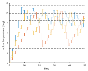
Figure 2: Three possible evolutions of the CPS of Example 2.

II-A Labelled transition semantics

TABLE I: LTS for processes

$$\begin{array}[]{l@{\hspace*{10mm}}l}{\mbox{\small(Outp)}}\>\;\begin{array}[]{c}-\\[2.0pt] \hline\cr{\mathsf{timeout}\lfloor\mathsf{snd}\,c\langle{v}\rangle.P\rfloor Q}\mathrel{\;\raisebox{0.0pt}{$\stackrel{{\scriptstyle\,\overline{c}v}}{{\makebox[16.31091pt]{\rule{0.0pt}{4.30554pt}\mbox{}\leavevmode\xleaders\hbox{$\mkern-2.6mu\relbar\mkern-2.6mu$}\hfill\mbox{}}}}$}\rightarrow}P\end{array}\hfil\hskip 28.45274pt&{\mbox{\small(Inpp)}}\>\;\begin{array}[]{c}-\\[2.0pt] \hline\cr{\mathsf{timeout}\lfloor\mathsf{rcv}\,c({x}).P\rfloor Q}\mathrel{\;\raisebox{0.0pt}{$\stackrel{{\scriptstyle\,cv}}{{\makebox[14.34018pt]{\rule{0.0pt}{4.30554pt}\mbox{}\leavevmode\xleaders\hbox{$\mkern-2.6mu\relbar\mkern-2.6mu$}\hfill\mbox{}}}}$}\rightarrow}{P{\{^{v}\!/\!_{x}\}}}\end{array}\\[12.0pt] {\mbox{\small(Com)}}\>\;\begin{array}[]{c}P\mathrel{\;\raisebox{0.0pt}{$\stackrel{{\scriptstyle\,\overline{c}v}}{{\makebox[16.31091pt]{\rule{0.0pt}{4.30554pt}\mbox{}\leavevmode\xleaders\hbox{$\mkern-2.6mu\relbar\mkern-2.6mu$}\hfill\mbox{}}}}$}\rightarrow}{P^{\prime}}\quad Q\mathrel{\;\raisebox{0.0pt}{$\stackrel{{\scriptstyle\,cv}}{{\makebox[14.34018pt]{\rule{0.0pt}{4.30554pt}\mbox{}\leavevmode\xleaders\hbox{$\mkern-2.6mu\relbar\mkern-2.6mu$}\hfill\mbox{}}}}$}\rightarrow}{Q^{\prime}}\\[2.0pt] \hline\cr P\parallel Q\mathrel{\;\raisebox{0.0pt}{$\stackrel{{\scriptstyle\,\tau}}{{\makebox[10.72676pt]{\rule{0.0pt}{4.30554pt}\mbox{}\leavevmode\xleaders\hbox{$\mkern-2.6mu\relbar\mkern-2.6mu$}\hfill\mbox{}}}}$}\rightarrow}{P^{\prime}\parallel Q^{\prime}}\end{array}\hfil\hskip 28.45274pt&{\mbox{\small(Par)}}\>\;\begin{array}[]{c}P\mathrel{\;\raisebox{0.0pt}{$\stackrel{{\scriptstyle\,\lambda}}{{\makebox[11.75003pt]{\rule{0.0pt}{4.30554pt}\mbox{}\leavevmode\xleaders\hbox{$\mkern-2.6mu\relbar\mkern-2.6mu$}\hfill\mbox{}}}}$}\rightarrow}P^{\prime}\quad\lambda\neq\mathsf{idle}\\[2.0pt] \hline\cr{P\parallel Q}\mathrel{\;\raisebox{0.0pt}{$\stackrel{{\scriptstyle\,\lambda}}{{\makebox[11.75003pt]{\rule{0.0pt}{4.30554pt}\mbox{}\leavevmode\xleaders\hbox{$\mkern-2.6mu\relbar\mkern-2.6mu$}\hfill\mbox{}}}}$}\rightarrow}{P^{\prime}\parallel Q}\end{array}\\[12.0pt] {\mbox{\small(Write)}}\>\;\begin{array}[]{c}\mu\in\{p,\mbox{\Lightning}p\}\\[2.0pt] \hline\cr{\mathsf{timeout}\lfloor\mathsf{write}\,\mu\langle v\rangle.P\rfloor Q}\mathrel{\;\raisebox{0.0pt}{$\stackrel{{\scriptstyle\,\mu!v}}{{\makebox[17.47318pt]{\rule{0.0pt}{4.30554pt}\mbox{}\leavevmode\xleaders\hbox{$\mkern-2.6mu\relbar\mkern-2.6mu$}\hfill\mbox{}}}}$}\rightarrow}P\end{array}\hfil\hskip 28.45274pt&{\mbox{\small(Read)}}\>\;\begin{array}[]{c}\mu\in\{p,\mbox{\Lightning}p\}\\[2.0pt] \hline\cr{\mathsf{timeout}\lfloor\mathsf{read}\,\mu(x).P\rfloor Q}\mathrel{\;\raisebox{0.0pt}{$\stackrel{{\scriptstyle\,\mu?v}}{{\makebox[18.83429pt]{\rule{0.0pt}{4.30554pt}\mbox{}\leavevmode\xleaders\hbox{$\mkern-2.6mu\relbar\mkern-2.6mu$}\hfill\mbox{}}}}$}\rightarrow}{P{\{^{v}\!/\!_{x}\}}}\end{array}\\[12.0pt] {\mbox{\small($\mbox{\Lightning}$SensWrite$\mbox{\,\Lightning}$)}}\>\;\begin{array}[]{c}P\mathrel{\;\raisebox{0.0pt}{$\stackrel{{\scriptstyle\,\mbox{\Lightning}s!v}}{{\makebox[21.78659pt]{\rule{0.0pt}{4.30554pt}\mbox{}\leavevmode\xleaders\hbox{$\mkern-2.6mu\relbar\mkern-2.6mu$}\hfill\mbox{}}}}$}\rightarrow}{P^{\prime}}\quad Q\mathrel{\;\raisebox{0.0pt}{$\stackrel{{\scriptstyle\,s?v}}{{\makebox[17.8977pt]{\rule{0.0pt}{4.30554pt}\mbox{}\leavevmode\xleaders\hbox{$\mkern-2.6mu\relbar\mkern-2.6mu$}\hfill\mbox{}}}}$}\rightarrow}{Q^{\prime}}\\[2.0pt] \hline\cr P\parallel Q\mathrel{\;\raisebox{0.0pt}{$\stackrel{{\scriptstyle\,\tau:s}}{{\makebox[21.50787pt]{\rule{0.0pt}{4.30554pt}\mbox{}\leavevmode\xleaders\hbox{$\mkern-2.6mu\relbar\mkern-2.6mu$}\hfill\mbox{}}}}$}\rightarrow}{P^{\prime}\parallel Q^{\prime}}\end{array}\hfil\hskip 28.45274pt&{\mbox{\small($\mbox{\Lightning}$ActRead$\mbox{\,\Lightning}$)}}\>\;\begin{array}[]{c}P\mathrel{\;\raisebox{0.0pt}{$\stackrel{{\scriptstyle\,a!v}}{{\makebox[16.95546pt]{\rule{0.0pt}{4.30554pt}\mbox{}\leavevmode\xleaders\hbox{$\mkern-2.6mu\relbar\mkern-2.6mu$}\hfill\mbox{}}}}$}\rightarrow}{P^{\prime}}\quad Q\mathrel{\;\raisebox{0.0pt}{$\stackrel{{\scriptstyle\,\mbox{\Lightning}a?v}}{{\makebox[23.56657pt]{\rule{0.0pt}{4.30554pt}\mbox{}\leavevmode\xleaders\hbox{$\mkern-2.6mu\relbar\mkern-2.6mu$}\hfill\mbox{}}}}$}\rightarrow}{Q^{\prime}}\\[2.0pt] \hline\cr P\parallel Q\mathrel{\;\raisebox{0.0pt}{$\stackrel{{\scriptstyle\,\tau:a}}{{\makebox[21.92674pt]{\rule{0.0pt}{4.30554pt}\mbox{}\leavevmode\xleaders\hbox{$\mkern-2.6mu\relbar\mkern-2.6mu$}\hfill\mbox{}}}}$}\rightarrow}{P^{\prime}\parallel Q^{\prime}}\end{array}\\[12.0pt] {\mbox{\small(Res)}}\>\;\begin{array}[]{c}P\mathrel{\;\raisebox{0.0pt}{$\stackrel{{\scriptstyle\,\lambda}}{{\makebox[11.75003pt]{\rule{0.0pt}{4.30554pt}\mbox{}\leavevmode\xleaders\hbox{$\mkern-2.6mu\relbar\mkern-2.6mu$}\hfill\mbox{}}}}$}\rightarrow}P^{\prime}\quad\lambda\not\in\{{cv},{\overline{c}v}\}\\[2.0pt] \hline\cr P{\setminus}c\mathrel{\;\raisebox{0.0pt}{$\stackrel{{\scriptstyle\,\lambda}}{{\makebox[11.75003pt]{\rule{0.0pt}{4.30554pt}\mbox{}\leavevmode\xleaders\hbox{$\mkern-2.6mu\relbar\mkern-2.6mu$}\hfill\mbox{}}}}$}\rightarrow}{P^{\prime}}{\setminus}c\end{array}\hfil\hskip 28.45274pt&{\mbox{\small(Rec)}}\>\;\begin{array}[]{c}P{\{^{\tilde{w}}\!/\!_{\tilde{x}}\}}\mathrel{\;\raisebox{0.0pt}{$\stackrel{{\scriptstyle\,\lambda}}{{\makebox[11.75003pt]{\rule{0.0pt}{4.30554pt}\mbox{}\leavevmode\xleaders\hbox{$\mkern-2.6mu\relbar\mkern-2.6mu$}\hfill\mbox{}}}}$}\rightarrow}Q\quad H(\tilde{x})=P\\[2.0pt] \hline\cr H\langle\tilde{w}\rangle\mathrel{\;\raisebox{0.0pt}{$\stackrel{{\scriptstyle\,\lambda}}{{\makebox[11.75003pt]{\rule{0.0pt}{4.30554pt}\mbox{}\leavevmode\xleaders\hbox{$\mkern-2.6mu\relbar\mkern-2.6mu$}\hfill\mbox{}}}}$}\rightarrow}Q\end{array}\\[12.0pt] {\mbox{\small(Then)}}\>\;\begin{array}[]{c}\llbracket b\rrbracket=\mathsf{true}\quad P\mathrel{\;\raisebox{0.0pt}{$\stackrel{{\scriptstyle\,\lambda}}{{\makebox[11.75003pt]{\rule{0.0pt}{4.30554pt}\mbox{}\leavevmode\xleaders\hbox{$\mkern-2.6mu\relbar\mkern-2.6mu$}\hfill\mbox{}}}}$}\rightarrow}P^{\prime}\\[2.0pt] \hline\cr\mathsf{if}\,(b)\,\{P\}\>\mathsf{else}\>\{Q\}\mathrel{\;\raisebox{0.0pt}{$\stackrel{{\scriptstyle\,\lambda}}{{\makebox[11.75003pt]{\rule{0.0pt}{4.30554pt}\mbox{}\leavevmode\xleaders\hbox{$\mkern-2.6mu\relbar\mkern-2.6mu$}\hfill\mbox{}}}}$}\rightarrow}P^{\prime}\end{array}\hfil\hskip 28.45274pt&{\mbox{\small(Else)}}\>\;\begin{array}[]{c}\llbracket b\rrbracket=\mathsf{false}\quad Q\mathrel{\;\raisebox{0.0pt}{$\stackrel{{\scriptstyle\,\lambda}}{{\makebox[11.75003pt]{\rule{0.0pt}{4.30554pt}\mbox{}\leavevmode\xleaders\hbox{$\mkern-2.6mu\relbar\mkern-2.6mu$}\hfill\mbox{}}}}$}\rightarrow}Q^{\prime}\\[2.0pt] \hline\cr\mathsf{if}\,(b)\,\{P\}\>\mathsf{else}\>\{Q\}\mathrel{\;\raisebox{0.0pt}{$\stackrel{{\scriptstyle\,\lambda}}{{\makebox[11.75003pt]{\rule{0.0pt}{4.30554pt}\mbox{}\leavevmode\xleaders\hbox{$\mkern-2.6mu\relbar\mkern-2.6mu$}\hfill\mbox{}}}}$}\rightarrow}Q^{\prime}\end{array}\\[12.0pt] {\mbox{\small(TimeNil)}}\>\;\begin{array}[]{c}-\\[2.0pt] \hline\cr\mathsf{nil}\mathrel{\;\raisebox{0.0pt}{$\stackrel{{\scriptstyle\,\mathsf{idle}}}{{\makebox[18.55559pt]{\rule{0.0pt}{4.30554pt}\mbox{}\leavevmode\xleaders\hbox{$\mkern-2.6mu\relbar\mkern-2.6mu$}\hfill\mbox{}}}}$}\rightarrow}\mathsf{nil}\end{array}\hfil\hskip 28.45274pt&{\mbox{\small(Delay)}}\>\;\begin{array}[]{c}-\\[2.0pt] \hline\cr{\mathsf{idle}.P}\mathrel{\;\raisebox{0.0pt}{$\stackrel{{\scriptstyle\,\mathsf{idle}}}{{\makebox[18.55559pt]{\rule{0.0pt}{4.30554pt}\mbox{}\leavevmode\xleaders\hbox{$\mkern-2.6mu\relbar\mkern-2.6mu$}\hfill\mbox{}}}}$}\rightarrow}P\end{array}\\[12.0pt] {\mbox{\small(Timeout)}}\>\;\begin{array}[]{c}-\\[2.0pt] \hline\cr{\mathsf{timeout}\lfloor\pi.P\rfloor Q}\mathrel{\;\raisebox{0.0pt}{$\stackrel{{\scriptstyle\,\mathsf{idle}}}{{\makebox[18.55559pt]{\rule{0.0pt}{4.30554pt}\mbox{}\leavevmode\xleaders\hbox{$\mkern-2.6mu\relbar\mkern-2.6mu$}\hfill\mbox{}}}}$}\rightarrow}Q\end{array}\hfil\hskip 28.45274pt&{\mbox{\small(TimePar)}}\>\;\begin{array}[]{c}P\mathrel{\;\raisebox{0.0pt}{$\stackrel{{\scriptstyle\,\mathsf{idle}}}{{\makebox[18.55559pt]{\rule{0.0pt}{4.30554pt}\mbox{}\leavevmode\xleaders\hbox{$\mkern-2.6mu\relbar\mkern-2.6mu$}\hfill\mbox{}}}}$}\rightarrow}{P^{\prime}}\quad Q\mathrel{\;\raisebox{0.0pt}{$\stackrel{{\scriptstyle\,\mathsf{idle}}}{{\makebox[18.55559pt]{\rule{0.0pt}{4.30554pt}\mbox{}\leavevmode\xleaders\hbox{$\mkern-2.6mu\relbar\mkern-2.6mu$}\hfill\mbox{}}}}$}\rightarrow}{Q^{\prime}}\\[2.0pt] \hline\cr{P\parallel Q}\mathrel{\;\raisebox{0.0pt}{$\stackrel{{\scriptstyle\,\mathsf{idle}}}{{\makebox[18.55559pt]{\rule{0.0pt}{4.30554pt}\mbox{}\leavevmode\xleaders\hbox{$\mkern-2.6mu\relbar\mkern-2.6mu$}\hfill\mbox{}}}}$}\rightarrow}{P^{\prime}\parallel Q^{\prime}}\end{array}\end{array}$$

In this section, we provide the dynamics of CCPSA in terms of a labelled transition system (LTS) in the SOS style of Plotkin. Definition 5 introduces auxiliary operators on environments.

Definition 5.

Let $E=\langle\xi_{\mathrm{x}}{},\xi_{\mathrm{u}}{},\xi_{\mathrm{w}}{},\mathit{evol}{},\xi_{\mathrm{e}}{},\mathit{meas}{},\mathit{inv}{},\mathit{safe}{}\rangle$.

• $\mathit{read\_sensor}(E,s)\;\stackrel{{\scriptstyle\operatorname{def}}}{{=}}\;\{\xi(s)\,:\,\xi\in\mathit{meas}{}(\xi_{\mathrm{x}}{},\xi_{\mathrm{e}}{})\}$,

• $\mathit{update\_act}(E,a,v)\;\stackrel{{\scriptstyle\operatorname{def}}}{{=}}\;E[\xi_{\mathrm{u}}{}\leftarrow\xi_{\mathrm{u}}{}[a\mapsto v]]$,

• $\mathit{next}(E)\;\stackrel{{\scriptstyle\operatorname{def}}}{{=}}\;\bigcup_{\scriptsize\xi\in\mathit{evol}{}(\xi_{\mathrm{x}}{},\xi_{\mathrm{u}}{},\xi_{\mathrm{w}}{})}\{E[\xi_{\mathrm{x}}{}\leftarrow\xi]\}$,

• $\mathit{inv}{}(E)\;\stackrel{{\scriptstyle\operatorname{def}}}{{=}}\;\mathit{inv}{}(\xi_{\mathrm{x}}{})$,

• $\mathit{safe}{}(E)\;\stackrel{{\scriptstyle\operatorname{def}}}{{=}}\;\mathit{safe}{}(\xi_{\mathrm{x}}{})$.

The operator $\mathit{read\_sensor}(E,s)$ returns the set of possible measurements detected by sensor $s$ in the environment $E$; it returns a set of possible values rather than a single value due to the error $\xi_{\mathrm{e}}{}(s)$ of sensor $s$. $\mathit{update\_act}(E,a,v)$ returns the new environment in which the actuator function is updated in such a manner to associate the actuator $a$ with the value $v$. $\mathit{next}(E)$ returns the set of the next admissible environments reachable from $E$, by an application of $\mathit{evol}{}$. $\mathit{inv}{}(E)$ checks whether the invariant is satisfied by the current values of the state variables (here, abusing notation, we overload the meaning of the function $\mathit{inv}{}$). $\mathit{safe}{}(E)$ checks whether the safety conditions are satisfied by the current values of the state variables.

TABLE II: LTS for CPSs

$${\small\begin{array}[]{c}{\mbox{\small(Out)}}\>\;\begin{array}[]{c}P\mathrel{\;\raisebox{0.0pt}{$\stackrel{{\scriptstyle\,\overline{c}v}}{{\makebox[15.17986pt]{\rule{0.0pt}{3.87498pt}\mbox{}\leavevmode\xleaders\hbox{$\mkern-2.6mu\relbar\mkern-2.6mu$}\hfill\mbox{}}}}$}\rightarrow}P^{\prime}\quad\operatorname{inv}(E)\\[2.0pt] \hline\cr E\,{\Join_{\cal S}}\,P\mathrel{\;\raisebox{0.0pt}{$\stackrel{{\scriptstyle\,\overline{c}v}}{{\makebox[15.17986pt]{\rule{0.0pt}{3.87498pt}\mbox{}\leavevmode\xleaders\hbox{$\mkern-2.6mu\relbar\mkern-2.6mu$}\hfill\mbox{}}}}$}\rightarrow}E\,{\Join_{\cal S}}\,P^{\prime}\end{array}\quad\quad\quad\quad{\mbox{\small(Inp)}}\>\;\begin{array}[]{c}P\mathrel{\;\raisebox{0.0pt}{$\stackrel{{\scriptstyle\,cv}}{{\makebox[12.9062pt]{\rule{0.0pt}{3.87498pt}\mbox{}\leavevmode\xleaders\hbox{$\mkern-2.6mu\relbar\mkern-2.6mu$}\hfill\mbox{}}}}$}\rightarrow}P^{\prime}\quad\operatorname{inv}(E)\\[2.0pt] \hline\cr E\,{\Join_{\cal S}}\,P\mathrel{\;\raisebox{0.0pt}{$\stackrel{{\scriptstyle\,cv}}{{\makebox[12.9062pt]{\rule{0.0pt}{3.87498pt}\mbox{}\leavevmode\xleaders\hbox{$\mkern-2.6mu\relbar\mkern-2.6mu$}\hfill\mbox{}}}}$}\rightarrow}E\,{\Join_{\cal S}}\,P^{\prime}\end{array}\\[13.0pt] {\mbox{\small(SensReadSec)}}\>\;\begin{array}[]{c}P\mathrel{\;\raisebox{0.0pt}{$\stackrel{{\scriptstyle\,s?v}}{{\makebox[16.10797pt]{\rule{0.0pt}{3.87498pt}\mbox{}\leavevmode\xleaders\hbox{$\mkern-2.6mu\relbar\mkern-2.6mu$}\hfill\mbox{}}}}$}\rightarrow}P^{\prime}\quad s\in{\cal S}\quad\operatorname{inv}(E)\quad\mbox{\small{$v\in\operatorname{read\_sensor}(E,s)$}}\\[2.0pt] \hline\cr E\,{\Join_{\cal S}}\,P\mathrel{\;\raisebox{0.0pt}{$\stackrel{{\scriptstyle\,\tau}}{{\makebox[9.65413pt]{\rule{0.0pt}{3.87498pt}\mbox{}\leavevmode\xleaders\hbox{$\mkern-2.6mu\relbar\mkern-2.6mu$}\hfill\mbox{}}}}$}\rightarrow}E\,{\Join_{\cal S}}\,P^{\prime}\end{array}\\[13.0pt] {\mbox{\small(SensReadUnsec)}}\>\;\begin{array}[]{c}P\mathrel{\;\raisebox{0.0pt}{$\stackrel{{\scriptstyle\,s?v}}{{\makebox[16.10797pt]{\rule{0.0pt}{3.87498pt}\mbox{}\leavevmode\xleaders\hbox{$\mkern-2.6mu\relbar\mkern-2.6mu$}\hfill\mbox{}}}}$}\rightarrow}P^{\prime}\quad s\not\in{\cal S}\quad P\mathrel{{\mathrel{\;\raisebox{0.0pt}{$\stackrel{{\scriptstyle\,\mbox{\Lightning}s!v}}{{\makebox[19.60796pt]{\rule{0.0pt}{3.87498pt}\mbox{}\leavevmode\xleaders\hbox{$\mkern-2.6mu\relbar\mkern-2.6mu$}\hfill\mbox{}}}}$}\rightarrow}}\makebox[0.0pt][r]{$\not$\hskip 7.74997pt}}{\!}\quad\operatorname{inv}(E)\quad\mbox{\small{$v\in\operatorname{read\_sensor}(E,s)$}}\\[2.0pt] \hline\cr E\,{\Join_{\cal S}}\,P\mathrel{\;\raisebox{0.0pt}{$\stackrel{{\scriptstyle\,\tau}}{{\makebox[9.65413pt]{\rule{0.0pt}{3.87498pt}\mbox{}\leavevmode\xleaders\hbox{$\mkern-2.6mu\relbar\mkern-2.6mu$}\hfill\mbox{}}}}$}\rightarrow}E\,{\Join_{\cal S}}\,P^{\prime}\end{array}\\[13.0pt] {\mbox{\small($\mbox{\Lightning}$SensRead$\mbox{\,\Lightning}$)}}\>\;\begin{array}[]{c}P\mathrel{\;\raisebox{0.0pt}{$\stackrel{{\scriptstyle\,\mbox{\Lightning}s?v}}{{\makebox[20.83296pt]{\rule{0.0pt}{3.87498pt}\mbox{}\leavevmode\xleaders\hbox{$\mkern-2.6mu\relbar\mkern-2.6mu$}\hfill\mbox{}}}}$}\rightarrow}P^{\prime}\quad s\not\in{\cal S}\quad\operatorname{inv}(E)\quad\mbox{\small{$v\in\operatorname{read\_sensor}(E,s)$}}\\[2.0pt] \hline\cr E\,{\Join_{\cal S}}\,P\mathrel{\;\raisebox{0.0pt}{$\stackrel{{\scriptstyle\,\tau}}{{\makebox[9.65413pt]{\rule{0.0pt}{3.87498pt}\mbox{}\leavevmode\xleaders\hbox{$\mkern-2.6mu\relbar\mkern-2.6mu$}\hfill\mbox{}}}}$}\rightarrow}E\,{\Join_{\cal S}}\,P^{\prime}\end{array}\\[13.0pt] {\mbox{\small(ActWriteSec)}}\>\;\begin{array}[]{c}P\mathrel{\;\raisebox{0.0pt}{$\stackrel{{\scriptstyle\,a!v}}{{\makebox[15.25995pt]{\rule{0.0pt}{3.87498pt}\mbox{}\leavevmode\xleaders\hbox{$\mkern-2.6mu\relbar\mkern-2.6mu$}\hfill\mbox{}}}}$}\rightarrow}{P^{\prime}}\quad a\in{\cal S}\quad\operatorname{inv}(E)\quad{E^{\prime}}=\operatorname{update\_act}(E,a,v)\\[2.0pt] \hline\cr E\,{\Join_{\cal S}}\,P\mathrel{\;\raisebox{0.0pt}{$\stackrel{{\scriptstyle\,\tau}}{{\makebox[9.65413pt]{\rule{0.0pt}{3.87498pt}\mbox{}\leavevmode\xleaders\hbox{$\mkern-2.6mu\relbar\mkern-2.6mu$}\hfill\mbox{}}}}$}\rightarrow}E^{\prime}\,{\Join_{\cal S}}\,P^{\prime}\end{array}\\[13.0pt] {\mbox{\small(ActWriteUnsec)}}\>\;\begin{array}[]{c}P\mathrel{\;\raisebox{0.0pt}{$\stackrel{{\scriptstyle\,a!v}}{{\makebox[15.25995pt]{\rule{0.0pt}{3.87498pt}\mbox{}\leavevmode\xleaders\hbox{$\mkern-2.6mu\relbar\mkern-2.6mu$}\hfill\mbox{}}}}$}\rightarrow}{P^{\prime}}\quad a\not\in{\cal S}\quad P\mathrel{{\mathrel{\;\raisebox{0.0pt}{$\stackrel{{\scriptstyle\,\mbox{\Lightning}a?v}}{{\makebox[21.20995pt]{\rule{0.0pt}{3.87498pt}\mbox{}\leavevmode\xleaders\hbox{$\mkern-2.6mu\relbar\mkern-2.6mu$}\hfill\mbox{}}}}$}\rightarrow}}\makebox[0.0pt][r]{$\not$\hskip 7.74997pt}}{\!}\quad\operatorname{inv}(E)\quad{E^{\prime}}=\operatorname{update\_act}(E,a,v)\\[2.0pt] \hline\cr E\,{\Join_{\cal S}}\,P\mathrel{\;\raisebox{0.0pt}{$\stackrel{{\scriptstyle\,\tau}}{{\makebox[9.65413pt]{\rule{0.0pt}{3.87498pt}\mbox{}\leavevmode\xleaders\hbox{$\mkern-2.6mu\relbar\mkern-2.6mu$}\hfill\mbox{}}}}$}\rightarrow}E^{\prime}\,{\Join_{\cal S}}\,P^{\prime}\end{array}\\[13.0pt] {\mbox{\small($\mbox{\Lightning}$ActWrite$\mbox{\,\Lightning}$)}}\>\;\begin{array}[]{c}P\mathrel{\;\raisebox{0.0pt}{$\stackrel{{\scriptstyle\,\mbox{\Lightning}a!v}}{{\makebox[19.98494pt]{\rule{0.0pt}{3.87498pt}\mbox{}\leavevmode\xleaders\hbox{$\mkern-2.6mu\relbar\mkern-2.6mu$}\hfill\mbox{}}}}$}\rightarrow}{P^{\prime}}\quad a\not\in{\cal S}\quad\operatorname{inv}(E)\quad{E^{\prime}}=\operatorname{update\_act}(E,a,v)\\[2.0pt] \hline\cr E\,{\Join_{\cal S}}\,P\mathrel{\;\raisebox{0.0pt}{$\stackrel{{\scriptstyle\,\tau}}{{\makebox[9.65413pt]{\rule{0.0pt}{3.87498pt}\mbox{}\leavevmode\xleaders\hbox{$\mkern-2.6mu\relbar\mkern-2.6mu$}\hfill\mbox{}}}}$}\rightarrow}E^{\prime}\,{\Join_{\cal S}}\,P^{\prime}\end{array}\\[13.0pt] {\mbox{\small(Tau)}}\>\;\begin{array}[]{c}(P\mathrel{\;\raisebox{0.0pt}{$\stackrel{{\scriptstyle\,\tau}}{{\makebox[9.65413pt]{\rule{0.0pt}{3.87498pt}\mbox{}\leavevmode\xleaders\hbox{$\mkern-2.6mu\relbar\mkern-2.6mu$}\hfill\mbox{}}}}$}\rightarrow}P^{\prime})\vee(P\mathrel{\;\raisebox{0.0pt}{$\stackrel{{\scriptstyle\,\tau:p}}{{\makebox[19.57382pt]{\rule{0.0pt}{3.87498pt}\mbox{}\leavevmode\xleaders\hbox{$\mkern-2.6mu\relbar\mkern-2.6mu$}\hfill\mbox{}}}}$}\rightarrow}P^{\prime}\>\;p\not\in{\cal S})\quad\operatorname{inv}(E)\\[2.0pt] \hline\cr E\,{\Join_{\cal S}}\,P\mathrel{\;\raisebox{0.0pt}{$\stackrel{{\scriptstyle\,\tau}}{{\makebox[9.65413pt]{\rule{0.0pt}{3.87498pt}\mbox{}\leavevmode\xleaders\hbox{$\mkern-2.6mu\relbar\mkern-2.6mu$}\hfill\mbox{}}}}$}\rightarrow}E\,{\Join_{\cal S}}\,P^{\prime}\end{array}\quad\quad{\mbox{\small(Deadlock)}}\>\;\begin{array}[]{c}\neg\operatorname{inv}(E)\\[2.0pt] \hline\cr E\,{\Join_{\cal S}}\,P\mathrel{\;\raisebox{0.0pt}{$\stackrel{{\scriptstyle\,\mathsf{deadlock}}}{{\makebox[30.87509pt]{\rule{0.0pt}{3.87498pt}\mbox{}\leavevmode\xleaders\hbox{$\mkern-2.6mu\relbar\mkern-2.6mu$}\hfill\mbox{}}}}$}\rightarrow}E\,{\Join_{\cal S}}\,P\end{array}\\[13.0pt] {\mbox{\small(Time)}}\>\;\begin{array}[]{c}P\mathrel{\;\raisebox{0.0pt}{$\stackrel{{\scriptstyle\,\mathsf{idle}}}{{\makebox[16.70006pt]{\rule{0.0pt}{3.87498pt}\mbox{}\leavevmode\xleaders\hbox{$\mkern-2.6mu\relbar\mkern-2.6mu$}\hfill\mbox{}}}}$}\rightarrow}{P^{\prime}}\quad E\,{\Join_{\cal S}}\,P\mathrel{{\mathrel{\;\raisebox{0.0pt}{$\stackrel{{\scriptstyle\,\tau}}{{\makebox[9.65413pt]{\rule{0.0pt}{3.87498pt}\mbox{}\leavevmode\xleaders\hbox{$\mkern-2.6mu\relbar\mkern-2.6mu$}\hfill\mbox{}}}}$}\rightarrow}}\makebox[0.0pt][r]{$\not$\hskip 7.74997pt}}{\!}\quad\operatorname{inv}(E)\quad E^{\prime}\in\operatorname{next}(E)\\[2.0pt] \hline\cr E\,{\Join_{\cal S}}\,P\mathrel{\;\raisebox{0.0pt}{$\stackrel{{\scriptstyle\,\mathsf{idle}}}{{\makebox[16.70006pt]{\rule{0.0pt}{3.87498pt}\mbox{}\leavevmode\xleaders\hbox{$\mkern-2.6mu\relbar\mkern-2.6mu$}\hfill\mbox{}}}}$}\rightarrow}E^{\prime}\,{\Join_{\cal S}}\,P^{\prime}\end{array}\quad\quad{\mbox{\small(Safety)}}\>\;\begin{array}[]{c}\neg\operatorname{safe}(E)\quad\operatorname{inv}(E)\\[2.0pt] \hline\cr E\,{\Join_{\cal S}}\,P\mathrel{\;\raisebox{0.0pt}{$\stackrel{{\scriptstyle\,\mathsf{unsafe}}}{{\makebox[24.26007pt]{\rule{0.0pt}{3.87498pt}\mbox{}\leavevmode\xleaders\hbox{$\mkern-2.6mu\relbar\mkern-2.6mu$}\hfill\mbox{}}}}$}\rightarrow}E\,{\Join_{\cal S}}\,P\end{array}\end{array}}$$

In Table I, we provide transition rules for processes. Here, the meta-variable $\lambda$ ranges over labels in the set $\{\mathsf{idle},\tau,{\overline{c}v},{cv},\allowbreak a!v,s?v,\mbox{\Lightning}p!v,\mbox{\Lightning}p?v,\tau{:}p\}$. Rules (Outp), (Inpp) and (Com) serve to model channel communication, on some channel $c$. Rules (Write) and (Read) denote the writing/reading of some data on the physical device $p$. Rule (↯SensWrite ↯) models an integrity attack on sensor $s$, where the controller of $s$ is supplied with a fake value $v$ provided by the attack. Rule (↯ActRead ↯) models a DoS attack to the actuator $a$, where the update request of the controller is intercepted by the attacker and it never reaches the actuator. Rule (Par) propagates untimed actions over parallel components. Rules (Res), (Rec), (Then) and (Else) are standard. The following four rules model the passage of time. The symmetric counterparts of rules (Com) and (Par) are omitted.

In Table II, we lift the transition rules from processes to systems. Except for rule (Deadlock), all rules have a common premise $\mathit{inv}{}(E)$: a system can evolve only if the invariant is satisfied. Here, actions, ranged over by $\alpha$, are in the set $\{\tau,{\overline{c}v},{cv},\mathsf{idle},\mathsf{deadlock},\mathsf{unsafe}\}$. These actions denote: internal activities ($\tau$); logical activities, more precisely, channel transmission (${\overline{c}v}$ and ${cv}$); the passage of time ($\mathsf{idle}$); and two specific physical events: system deadlock ($\mathsf{deadlock}$) and the violation of the safety conditions ($\mathsf{unsafe}$). Rules (Out) and (Inp) model transmission and reception, with an external system, on a channel $c$. Rule (SensReadSec) models the reading of the current data detected at a secured sensor $s$, whereas rule (SensReadUnsec) models the reading of an unsecured sensor $s$. In this case, since the sensor is not secured, the presence of a malicious action $\mbox{\Lightning}s!w$ prevents the reading of the sensor. We already said that rule (↯SensWrite ↯) of Table I models integrity attacks on an unsecured sensor $s$, however, together with rule (SensReadUnsec), it also serves to model DoS attacks on an unsecured sensor $s$, as the controller of $s$ cannot read its correct value if the attacker is currently supplying a fake value for it.

Rule (↯SensRead ↯) allows the attacker to read the confidential value detected at an unsecured sensor $s$. Rule (ActWriteSec) models the writing of a value $v$ on a secured actuator $a$, whereas rule (ActWriteUnsec) models the writing on a unsecured actuator $a$. Again, if the actuator is unsecured, the presence of an attack (capable of performing an action $\mbox{\Lightning}a?v$) prevents the correct access to the actuator by the controller. Rule (↯ActWrite ↯) models an integrity attack to an unsecured actuator $a$, where the attack updates the actuator with a fake value.

Note that our operational semantics ensures a preemptive power to prefixes of the form $\mathsf{write}\,\mbox{\Lightning}p\langle v\rangle$ and $\mathsf{read}\,\mbox{\Lightning}p(x)$ on unsecured devices $p$. This because an attack process can always prevent the regular access to a unsecured physical device (sensor or actuator) by its controller.

Proposition 1 (Attack preemptiveness).

Let $M\allowbreak=E\,{\Join_{\cal S}}\,P$.

• If there is $Q$ such that $P\mathrel{\;\raisebox{0.0pt}{$\stackrel{{\scriptstyle\,\mbox{\Lightning}s!v}}{{\makebox[21.78659pt]{\rule{0.0pt}{4.30554pt}\mbox{}\leavevmode\xleaders\hbox{$\mkern-2.6mu\relbar\mkern-2.6mu$}\hfill\mbox{}}}}$}\rightarrow}Q$, with $s\not\in{\cal S}$, then there is no $M^{\prime}$ such that $M\mathrel{\;\raisebox{0.0pt}{$\stackrel{{\scriptstyle\,\tau}}{{\makebox[10.72676pt]{\rule{0.0pt}{4.30554pt}\mbox{}\leavevmode\xleaders\hbox{$\mkern-2.6mu\relbar\mkern-2.6mu$}\hfill\mbox{}}}}$}\rightarrow}M^{\prime}$ by an application of the rule (SensReadUnsec).

• If there is $Q$ such that $P\mathrel{\;\raisebox{0.0pt}{$\stackrel{{\scriptstyle\,\mbox{\Lightning}a?v}}{{\makebox[23.56657pt]{\rule{0.0pt}{4.30554pt}\mbox{}\leavevmode\xleaders\hbox{$\mkern-2.6mu\relbar\mkern-2.6mu$}\hfill\mbox{}}}}$}\rightarrow}Q$, with $a\not\in{\cal S}$, then there is no $M^{\prime}$ such that $M\mathrel{\;\raisebox{0.0pt}{$\stackrel{{\scriptstyle\,\tau}}{{\makebox[10.72676pt]{\rule{0.0pt}{4.30554pt}\mbox{}\leavevmode\xleaders\hbox{$\mkern-2.6mu\relbar\mkern-2.6mu$}\hfill\mbox{}}}}$}\rightarrow}M^{\prime}$ by an application of the rule (ActWriteUnsec).

Rule (Tau) lifts non-observable actions from processes to systems. This includes communications channels and attacks’ accesses to unsecured physical devices. A similar lifting occurs in rule (Time) for timed actions, where $\operatorname{next}(E)$ returns the set of possible environments for the next time slot. Thus, by an application of rule (Time) a CPS moves to the next physical state, in the next time slot. Rule (Deadlock) is introduced to signal the violation of the invariant. When the invariant is violated, a system deadlock occurs and then, in CCPSA, the system emits a special action $\mathsf{deadlock}$, forever. Similarly, rule (Safety) is introduced to detect the violation of safety conditions. In this case, the system may emit a special action $\mathsf{unsafe}$ and then continue its evolution.

Now, having defined the actions that can be performed by a system, we can easily concatenate these actions to define the possible execution traces of the system. Formally, given a trace $t=\alpha_{1}\ldots\alpha_{n}$, we will write $\mathrel{\;\raisebox{0.0pt}{$\stackrel{{\scriptstyle\,t}}{{\makebox[10.19447pt]{\rule{0.0pt}{4.30554pt}\mbox{}\leavevmode\xleaders\hbox{$\mkern-2.6mu\relbar\mkern-2.6mu$}\hfill\mbox{}}}}$}\rightarrow}$ as an abbreviation for $\mathrel{\;\raisebox{0.0pt}{$\stackrel{{\scriptstyle\,\alpha_{1}}}{{\makebox[14.14459pt]{\rule{0.0pt}{4.30554pt}\mbox{}\leavevmode\xleaders\hbox{$\mkern-2.6mu\relbar\mkern-2.6mu$}\hfill\mbox{}}}}$}\rightarrow}\ldots\mathrel{\;\raisebox{0.0pt}{$\stackrel{{\scriptstyle\,\alpha_{n}}}{{\makebox[14.54553pt]{\rule{0.0pt}{4.30554pt}\mbox{}\leavevmode\xleaders\hbox{$\mkern-2.6mu\relbar\mkern-2.6mu$}\hfill\mbox{}}}}$}\rightarrow}$. In the following, we will use the function $\#\mathsf{idle}(t)$ to get the number of occurrences of the action $\mathsf{idle}$ in $t$.

The notion of trace allows us to provide a formal definition of soundness for CPSs: a CPS is said to be sound if it never deadlocks and never violates the safety conditions.

Definition 6 (System soundness).

Let $M$ be a well-formed CPS. We say that $M$ is sound if whenever $M\mathrel{\;\raisebox{0.0pt}{$\stackrel{{\scriptstyle\,t}}{{\makebox[10.19447pt]{\rule{0.0pt}{4.30554pt}\mbox{}\leavevmode\xleaders\hbox{$\mkern-2.6mu\relbar\mkern-2.6mu$}\hfill\mbox{}}}}$}\rightarrow}M^{\prime}$, for some $t$, both actions $\mathsf{deadlock}$ and $\mathsf{unsafe}$ never occur in $t$.

In our security analysis, we will focus on sound CPSs. For instance, Proposition 2 says that our running example $\mathit{Sys}$ is sound and it never transmits on the channel $\mathit{alarm}$.

Proposition 2.

Let $\mathit{Sys}$ be the CPS defined in Example 2. If $\mathit{Sys}\mathrel{\;\raisebox{0.0pt}{$\stackrel{{\scriptstyle\,t}}{{\makebox[10.19447pt]{\rule{0.0pt}{4.30554pt}\mbox{}\leavevmode\xleaders\hbox{$\mkern-2.6mu\relbar\mkern-2.6mu$}\hfill\mbox{}}}}$}\rightarrow}\mathit{Sys}^{\prime}$, for some trace $t{=}\alpha_{1}\ldots\alpha_{n}$, then $\alpha_{i}\in\{\tau,\mathsf{idle}\}$, for any $i\in\{1,\ldots,n\}$.

Actually, we can be quite precise on the temperature reached by $\mathit{Sys}$ before and after the cooling: in each of the $5$ rounds of cooling, the temperature will drop of a value laying in the real interval $[1{-}\delta,1{+}\delta]$, where $\delta$ is the uncertainty.

Proposition 3.

Let $\mathit{Sys}$ be the CPS defined in Example 2. For any execution trace of $\mathit{Sys}$, we have:

• when $\mathit{Sys}$ turns on the cooling, the value of the state variable $\mathit{temp}$ ranges over $(9.9\,,\,11.5]$;

• when $\mathit{Sys}$ turns off the cooling, the value of the variable $\mathit{temp}$ ranges over $(2.9,8.5]$.

II-B Behavioural semantics

We recall that the observable activities in CCPSA are: time passing, system deadlock, violation of safety conditions, and channel communication. Having defined a labelled transition semantics, we are ready to formalise our behavioural semantics, based on execution traces.

We adopt a standard notation for weak transitions: we write $\mathrel{\;\raisebox{0.0pt}{$\stackrel{{\scriptstyle\,}}{{\makebox[7.66669pt]{\mbox{}\leavevmode\xleaders\hbox{$\mkern-2.6mu\Relbar\mkern-2.6mu$}\hfill\mbox{}}}}$}\Rightarrow}$ for $(\mathrel{\;\raisebox{0.0pt}{$\stackrel{{\scriptstyle\,\tau}}{{\makebox[10.72676pt]{\rule{0.0pt}{4.30554pt}\mbox{}\leavevmode\xleaders\hbox{$\mkern-2.6mu\relbar\mkern-2.6mu$}\hfill\mbox{}}}}$}\rightarrow})^{*}$, whereas $\mathrel{\;\raisebox{0.0pt}{$\stackrel{{\scriptstyle\,\alpha}}{{\makebox[12.14459pt]{\mbox{}\leavevmode\xleaders\hbox{$\mkern-2.6mu\Relbar\mkern-2.6mu$}\hfill\mbox{}}}}$}\Rightarrow}$ means $\Longrightarrow\mathrel{\;\raisebox{0.0pt}{$\stackrel{{\scriptstyle\,\alpha}}{{\makebox[12.14459pt]{\rule{0.0pt}{4.30554pt}\mbox{}\leavevmode\xleaders\hbox{$\mkern-2.6mu\relbar\mkern-2.6mu$}\hfill\mbox{}}}}$}\rightarrow}\Longrightarrow$, and finally $\stackrel{{\scriptstyle\,{\hat{\alpha}}\,}}{{\Longrightarrow}}$ denotes $\mathrel{\;\raisebox{0.0pt}{$\stackrel{{\scriptstyle\,}}{{\makebox[7.66669pt]{\mbox{}\leavevmode\xleaders\hbox{$\mkern-2.6mu\Relbar\mkern-2.6mu$}\hfill\mbox{}}}}$}\Rightarrow}$ if $\alpha=\tau$ and $\stackrel{{\scriptstyle\,{\alpha}\,}}{{\Longrightarrow}}$ otherwise. Given a trace $t=\alpha_{1}{\ldots}\alpha_{n}$, we write $\mathrel{\;\raisebox{0.0pt}{$\stackrel{{\scriptstyle\,t}}{{\makebox[10.19447pt]{\rule{0.0pt}{4.30554pt}\mbox{}\leavevmode\xleaders\hbox{$\mkern-2.6mu\relbar\mkern-2.6mu$}\hfill\mbox{}}}}$}\rightarrow}$ for $\mathrel{\;\raisebox{0.0pt}{$\stackrel{{\scriptstyle\,\alpha_{1}}}{{\makebox[14.14459pt]{\rule{0.0pt}{4.30554pt}\mbox{}\leavevmode\xleaders\hbox{$\mkern-2.6mu\relbar\mkern-2.6mu$}\hfill\mbox{}}}}$}\rightarrow}{\ldots}\mathrel{\;\raisebox{0.0pt}{$\stackrel{{\scriptstyle\,\alpha_{n}}}{{\makebox[14.54553pt]{\rule{0.0pt}{4.30554pt}\mbox{}\leavevmode\xleaders\hbox{$\mkern-2.6mu\relbar\mkern-2.6mu$}\hfill\mbox{}}}}$}\rightarrow}$, and $\mathrel{\;\raisebox{0.0pt}{$\stackrel{{\scriptstyle\,\hat{t}}}{{\makebox[13.22226pt]{\mbox{}\leavevmode\xleaders\hbox{$\mkern-2.6mu\Relbar\mkern-2.6mu$}\hfill\mbox{}}}}$}\Rightarrow}$ as an abbreviation for $\mathrel{\;\raisebox{0.0pt}{$\stackrel{{\scriptstyle\,\widehat{\alpha_{1}}}}{{\makebox[13.22226pt]{\mbox{}\leavevmode\xleaders\hbox{$\mkern-2.6mu\Relbar\mkern-2.6mu$}\hfill\mbox{}}}}$}\Rightarrow}{\ldots}\mathrel{\;\raisebox{0.0pt}{$\stackrel{{\scriptstyle\,\widehat{\alpha_{n}}}}{{\makebox[13.22226pt]{\mbox{}\leavevmode\xleaders\hbox{$\mkern-2.6mu\Relbar\mkern-2.6mu$}\hfill\mbox{}}}}$}\Rightarrow}$.

Definition 7 (Trace preorder).

We write $M\sqsubseteq N$ if whenever $M\mathrel{\;\raisebox{0.0pt}{$\stackrel{{\scriptstyle\,t}}{{\makebox[10.19447pt]{\rule{0.0pt}{4.30554pt}\mbox{}\leavevmode\xleaders\hbox{$\mkern-2.6mu\relbar\mkern-2.6mu$}\hfill\mbox{}}}}$}\rightarrow}M^{\prime}$, for some $t$, there is $N^{\prime}$ such that $N\mathrel{\;\raisebox{0.0pt}{$\stackrel{{\scriptstyle\,\hat{t}}}{{\makebox[13.22226pt]{\mbox{}\leavevmode\xleaders\hbox{$\mkern-2.6mu\Relbar\mkern-2.6mu$}\hfill\mbox{}}}}$}\Rightarrow}N^{\prime}$.

Remark 1.

Unlike standard trace semantics, our trace preorder is able to observe deadlock thanks to the presence of the rule (Deadlock) and the special action $\mathsf{deadlock}$: if $M\sqsubseteq N$ and $M$ eventually deadlocks then also $N$ must eventually deadlock.

As we are interested in examining timing aspects of attacks, such as beginning and duration, we propose a timed variant of $\sqsubseteq$ up to (a possibly infinite) time interval. Intuitively, we write $M\sqsubseteq_{m..n}N$ if the CPS $N$ simulates the execution traces of $M$, except for the time interval $m..n$.

Definition 8 (Trace preorder up to a time interval).

We write $M\sqsubseteq_{m..n}N$, for $m\in\mathbb{N}^{+}$ and $n\in\mathbb{N}^{+}\cup\infty$, with $m\leq n$, if the following conditions hold:

• $m$ is the minimum integer for which there is a trace $t$, with $\#\mathsf{idle}(t)=m-1$, such that $M\mathrel{\;\raisebox{0.0pt}{$\stackrel{{\scriptstyle\,t}}{{\makebox[10.19447pt]{\rule{0.0pt}{4.30554pt}\mbox{}\leavevmode\xleaders\hbox{$\mkern-2.6mu\relbar\mkern-2.6mu$}\hfill\mbox{}}}}$}\rightarrow}$ and $N\not\!\!\mathrel{\;\raisebox{0.0pt}{$\stackrel{{\scriptstyle\,\hat{t}}}{{\makebox[13.22226pt]{\mbox{}\leavevmode\xleaders\hbox{$\mkern-2.6mu\Relbar\mkern-2.6mu$}\hfill\mbox{}}}}$}\Rightarrow}$;

• $n$ is the infimum element of $\mathbb{N}^{+}\cup\infty$, $n\geq m$, such that whenever $M\mathrel{\;\raisebox{0.0pt}{$\stackrel{{\scriptstyle\,t_{1}}}{{\makebox[12.19447pt]{\rule{0.0pt}{4.30554pt}\mbox{}\leavevmode\xleaders\hbox{$\mkern-2.6mu\relbar\mkern-2.6mu$}\hfill\mbox{}}}}$}\rightarrow}M^{\prime}$, with $\#\mathsf{idle}(t_{1})=n-1$, there is $t_{2}$, with $\#\mathsf{idle}(t_{1})=\#\mathsf{idle}(t_{2})$, such that $N\mathrel{\;\raisebox{0.0pt}{$\stackrel{{\scriptstyle\,t_{2}}}{{\makebox[12.19447pt]{\rule{0.0pt}{4.30554pt}\mbox{}\leavevmode\xleaders\hbox{$\mkern-2.6mu\relbar\mkern-2.6mu$}\hfill\mbox{}}}}$}\rightarrow}N^{\prime}$, for some $N^{\prime}$, and $M^{\prime}\sqsubseteq N^{\prime}$.

In the second item, note that $\mathrm{inf}(\emptyset)=\infty$. Thus, if $M\sqsubseteq_{m..\infty}N$ then $N$ simulates $M$ only in the first $m-1$ time slots.

Finally, note that we could have equipped CCPSA with a (bi)simulation-based behavioural semantics rather than a trace-based one, as done in [2] for a core of CCPSA with no security features; however, our trace semantics is simpler than (bi)simulation and it is sensitive to deadlocks of CPSs. Thus, it is fully adequate for the purposes of this paper.

III Cyber-Physical Attacks

In this section, we use CCPSA to formalise a threat model where attacks can manipulate sensor and/or actuator signals in order to drive a sound CPS into an undesired state [19]. An attack may have different levels of access to physical devices depending on the model assumed. For example, it might be able to get read access to the sensors but not write access; or it might get write-only access to the actuators but not read-access. This level of granularity is very important to model precisely how attacks can affect a CPS [4]. For simplicity, in this paper we don’t represent attacks on communication channels as our focus is on attacks to physical devices.

The syntax of our cyber-physical attack is a slight restriction of that for processes: in terms of the form $\mathsf{timeout}\lfloor\pi.P\rfloor Q$, we require $\pi\in\{\mathsf{write}\,\mbox{\Lightning}p\langle v\rangle,\mathsf{read}\,\mbox{\Lightning}p(x)\}$. Thus, we provide a syntactic way to distinguish attacks from genuine processes.

Definition 9 (Honest system).

A CPS $E\,{\Join_{\cal S}}\,P$ is honest if $P$ is honest, where $P$ is honest if it does not contain prefixes of the form $\mathsf{write}\,\mbox{\Lightning}p\langle v\rangle$ or $\mathsf{read}\,\mbox{\Lightning}p(x)$.

We group cyber-physical attacks in classes that describe both the malicious activity and the timing aspects of the attack. Thus, let $\mathcal{I}$ be a set of malicious activities on a number of physical devices, $m\in\mathbb{N}^{+}$ be the time slot when an attack starts, and $n\in\mathbb{N}^{+}\cup\infty$ be the time slot when the attack ends, we say that an attack $A$ is of class $C\in[\mathcal{I}\rightarrow{\cal P}(m..n)]$ if: (1) all possible malicious actions of $A$ coincide with those contained in $\mathcal{I}$, (2) the first of those actions may occur in the $m$-th time slot (i.e., after $m{-}1$ $\mathsf{idle}$-actions), and (3) the last of those actions may occur in the $n$-th time slot (i.e., after $n{-}1$ $\mathsf{idle}$-actions). Actually, for $\iota\in\mathcal{I}$, $C(\iota)$ returns a (possibly empty) set of time instants when the attack tamper with the device $\iota$; this set is contained in $m..n$. A class $C$ is always a total function.

Definition 10 (Class of attacks).

Let ${\cal I}=\{\mbox{\Lightning}p?:p\in{\cal S}\cup{\cal A}\}\cup\{\mbox{\Lightning}p!\,:p\in{\cal S}\cup{\cal A}\}$ be the set of all possible malicious activities on physical devices. Let $m\in\mathbb{N}^{+}$, $n\in\mathbb{N}^{+}\cup\infty$, with $m\leq n$. An attack $A$ is of class $C\in[\mathcal{I}\rightarrow{\cal P}(m..n)]$ whenever:

• $C(\iota)=\{k:A\mathrel{\;\raisebox{0.0pt}{$\stackrel{{\scriptstyle\,t}}{{\makebox[9.17506pt]{\rule{0.0pt}{3.87498pt}\mbox{}\leavevmode\xleaders\hbox{$\mkern-2.6mu\relbar\mkern-2.6mu$}\hfill\mbox{}}}}$}\rightarrow}\mathrel{\;\raisebox{0.0pt}{$\stackrel{{\scriptstyle\,\iota v}}{{\makebox[12.40964pt]{\rule{0.0pt}{3.87498pt}\mbox{}\leavevmode\xleaders\hbox{$\mkern-2.6mu\relbar\mkern-2.6mu$}\hfill\mbox{}}}}$}\rightarrow}A^{\prime}\,\wedge\,k=\#\mathsf{idle}(t)+1\}$, for $\iota\in\mathcal{I}$;

• $m=\inf\{\,k\,:\,k\in C(\iota)\,\wedge\,\iota\in\mathcal{I}\,\}$;

• $n=\sup\{\,k\,:\,k\in C(\iota)\,\wedge\,\iota\in\mathcal{I}\,\}.$

According to the approach proposed in [6], we can say that an attack $A$ affects a sound CPS $M$ if the execution of the composed system $M\parallel A$ differs from that of the original system $M$, in an observable manner. Basically, a cyber-physical attack can influence the system under attack in at least two different ways:

• The system $M\parallel A$ might deadlock when $M$ may not; this means that the attack $A$ affects the availability of the system. We recall that in the context of CPSs, deadlock is a particular severe physical event.

• The system $M\parallel A$ might have non-genuine execution traces containing observables (violations of safety conditions or communications on channels) that cannot be reproduced by $M$; here the attack affects the integrity of the system behaviour.

Definition 11 (Attack tolerance/vulnerability).

Let $M$ be an honest and sound CPS. We say that $M$ is tolerant to an attack $A$ if $M\parallel A\,\sqsubseteq\,M$. We say $M$ is vulnerable to an attack $A$ if there is a time interval $m..n$, with $m\in\mathbb{N}^{+}$ and $n\in\mathbb{N}^{+}\cup\infty$, such that $M\parallel A\>\sqsubseteq_{m..n}\,M$.

Thus, if a system $M$ is vulnerable to an attack $A$ of class $C\in[\mathcal{I}\rightarrow{\cal P}(m..n)]$, during the time interval $m^{\prime}..n^{\prime}$, then the attack operates during the interval $m..n$ but it influences the system under attack in the time interval $m^{\prime}..n^{\prime}$ (obviously, $m^{\prime}\geq m$). If $n^{\prime}$ is finite we have a temporary attack, otherwise we have a permanent attack. Furthermore, if $m^{\prime}-n$ is big enough and $n-m$ is small, then we have a quick nasty attack that affects the system late enough to allow attack camouflages [8]. On the other hand, if $m^{\prime}$ is significantly smaller than $n$, then the attack affects the observable behaviour of the system well before its termination and the CPS has good chances of undertaking countermeasures to stop the attack. Finally, if $M\parallel A\mathrel{\;\raisebox{0.0pt}{$\stackrel{{\scriptstyle\,t}}{{\makebox[10.19447pt]{\rule{0.0pt}{4.30554pt}\mbox{}\leavevmode\xleaders\hbox{$\mkern-2.6mu\relbar\mkern-2.6mu$}\hfill\mbox{}}}}$}\rightarrow}\mathrel{\;\raisebox{0.0pt}{$\stackrel{{\scriptstyle\,\mathsf{deadlock}}}{{\makebox[34.30562pt]{\rule{0.0pt}{4.30554pt}\mbox{}\leavevmode\xleaders\hbox{$\mkern-2.6mu\relbar\mkern-2.6mu$}\hfill\mbox{}}}}$}\rightarrow}$, for some trace $t$, the attack $A$ is called lethal, as it is capable to halt (deadlock) the CPS $M$. This is obviously a permanent attack.

Note that, according to Definition 11, the tolerance (or vulnerability) of a CPS also depends on the capability of the $\mathit{IDS}$ component to detect and signal undesired physical behaviours. In fact, the $\mathit{IDS}$ component might be designed to detect abnormal physical behaviours going well further than deadlocks and violations of safety conditions.

In the following, we say that an attack is stealthy if it is able to drive the CPS under attack into an incorrect physical state (either deadlock or violation of the safety conditions) without being noticed by the $\mathit{IDS}$ component.

In the rest of this section, we present a number of different attacks to the CPS $\mathit{Sys}$ described in Example 2.

Example 3.

Consider the following DoS/Integrity attack on the (controller of) the actuator $\mathit{cool}$, of class $C\in[\mathcal{I}\rightarrow{\cal P}(m..m)]$ with $C(\mbox{\Lightning}cool?)=C(\mbox{\Lightning}cool!)=\{m\}$ and $C(\iota)=\emptyset$, for $\iota\not\in\{\mbox{\Lightning}cool?,\mbox{\Lightning}cool!\}$; we call the attack $A_{m}$:

$$\mathsf{idle}^{m{-}1}.\mathsf{timeout}\lfloor{\mathsf{read}\,\mbox{\Lightning}cool(x)}.\mathsf{if}(x{=}{\mathsf{off}})\{{\mathsf{write}\,\mbox{\Lightning}cool\langle\mathsf{off}\rangle}\}\rfloor.$$

Here, the attack $A_{m}$ operates exclusively in the $m$-th time slot, when it tries to steal the cooling command (on or off) coming from the controller, and fabricates a fake command to turn off the cooling system. In practice, if the controller sends a command to turn off the coolant, nothing bad will happen as the attack will put the same message back. When the controller sends (in the $m$-th time slot) a command to turn the cooling on, the attack will drop the command. We recall that the controller will turn on the cooling only if the sensed temperature is greater than $10$ (and hence $\mathit{temp}>9.9$); this may happen only if $m>8$. Since the command to turn the cooling on is never re-sent by $\mathit{Ctrl}$, the temperature will continue to rise, and after $4$ time units the system will violate the safety conditions emitting an action $\mathsf{unsafe}$, while the $\mathit{IDS}$ component will start sending alarms every $5$ time units, until the whole system deadlocks because the temperature reaches the threshold of $50$ degrees.

Proposition 4.

Let $\mathit{Sys}$ be the CPS defined in Example 2, and $A_{m}$ be the attack defined in Example 3. Then,

• $\mathit{Sys}\parallel A_{m}\;\sqsubseteq\;\mathit{Sys}$, for $m\leq 8$,

• $\mathit{Sys}\parallel A_{m}\;\>\sqsubseteq_{m{+}4..\infty}\;\mathit{Sys}$, for $m>8$.

In this case, the $\mathit{IDS}$ component of $\mathit{Sys}$ is effective enough to detect the attack with only one time unit delay.

Example 4.

Consider the following DoS/Integrity attack to the (controller of) sensor $s_{\mathrm{t}}$, of class $C\in[\mathcal{I}\rightarrow{\cal P}(2..\infty)]$ such that $C(\mbox{\Lightning}s_{\mathrm{t}}?)=\{2\}$, $C(\mbox{\Lightning}s_{\mathrm{t}}!)=2..\infty$ and $C(\iota)=\emptyset$, for $\iota\not\in\{\mbox{\Lightning}s_{\mathrm{t}}!,\mbox{\Lightning}s_{\mathrm{t}}?\}$:

$$\begin{array}[]{rcl}A&=&\mathsf{idle}.\mathsf{timeout}\lfloor\mathsf{read}\,\mbox{\Lightning}s_{\mathrm{t}}(x).B\langle x\rangle\rfloor{}\\ B(y)&=&\mathsf{timeout}\lfloor{\mathsf{write}\,\mbox{\Lightning}s_{\mathrm{t}}\langle y\rangle.\mathsf{idle}.B\langle y\rangle}\rfloor{B\langle y\rangle}\end{array}$$

Here, the attack $A$ does the following actions in sequence: (i) she sleeps for one time unit, (ii) in the following time slot, she reads the current temperature $v$ at sensor $s_{\mathrm{t}}$, and (iii) for the rest of her life, she keeps sending the same temperature $v$ to the controller of $s_{\mathrm{t}}$. In the presence of this attack, the process $\mathit{Ctrl}$ never activates the $\mathit{Cooling}$ component (and, hence, nor the $\mathit{IDS}$ component, which is the only one which could send an alarm) as it will always detect a temperature below $10$. Thus, the compound system $\mathit{Sys}\parallel A$ will move to an unsafe state until the invariant will be violated and the system will deadlock. Indeed, in the worst scenario, after $\lceil\frac{9.9}{1{+}\delta}\rceil=\lceil\frac{9.9}{1.4}\rceil=8$ $\mathsf{idle}$-actions (in the $9$-th time slot) the value of $\mathit{temp}$ will be above $9.9$, and after further $5$ $\mathsf{idle}$-actions (in the $14$-th time slot) the system will violate the safety conditions emitting an $\mathsf{unsafe}$ action. After $=\lceil\frac{50}{1.4}\rceil=36$ $\mathsf{idle}$-actions, in the $37$-th time slot, the invariant may be broken because the state variable $\mathit{temp}$ may reach $50.4$ degrees, and the system will also emit a $\mathsf{deadlock}$ action. Thus, $\mathit{Sys}\parallel A\;\sqsubseteq_{14..\infty}\;\mathit{Sys}$. This is a lethal attack, as it causes a shut down of the system. It is also a stealthy attack as it remains unnoticed until the end.

In this attack, the $\mathit{IDS}$ component is completely ineffective as the sensor used by the component is compromised, and there is not way for the $\mathit{IDS}$ to understand whether the sensor is under attack. A more sophisticated $\mathit{IDS}$ might have a representation of the plant to recognise abnormal evolutions of the sensed temperature. In such case, the $\mathit{IDS}$ might switch on a second sensor, hoping that this one has not been compromised yet. Another possibility for the designer of the CPS is to secure the sensor. Although this is not always possible, as encryption/decryption of all packets depends on energy constraints of the device.

Our semantics ensures that secured devices cannot be attacked, as stated by the following proposition.

Proposition 5.

Let $M=E\,{\Join_{\cal S}}\,P$ be an honest and sound CPS. Let $C\in[\mathcal{I}\rightarrow{\cal P}(m..n)]$, with $\{p:C(\mbox{\Lightning}p?)\cup C(\mbox{\Lightning}p!)\neq\emptyset\}\subseteq\cal S$. Then $M\parallel A\sqsubseteq M$, for any attack $A$ of class $C$.

Now, let us examine a similar but less severe attack.

Example 5.

Consider the following DoS/Integrity attack to the controller of sensor $s_{\mathrm{t}}$, of class $C\in[\mathcal{I}\rightarrow{\cal P}(1..n)]$, for $n>0$, with $C(\mbox{\Lightning}s_{\mathrm{t}}!)=C(\mbox{\Lightning}s_{\mathrm{t}}?)=1..n$ and $C(\iota)=\emptyset$, for $\iota\not\in\{\mbox{\Lightning}s_{\mathrm{t}}!,\mbox{\Lightning}s_{\mathrm{t}}?\}$:

$$\begin{array}[]{rcl}A_{n}&=&\mathsf{timeout}\lfloor\mathsf{read}\,\mbox{\Lightning}s_{\mathrm{t}}(x).\mathsf{timeout}\lfloor\{\mathsf{write}\,\mbox{\Lightning}s_{\mathrm{t}}\langle x{-}2\rangle.\\ &&\mathsf{idle}.A_{n-1}\rfloor{A_{n-1}}\rfloor{A_{n-1}}\end{array}$$

with $A_{0}=\mathsf{nil}$. In this attack, for $n$ consecutive time slots, $A_{n}$ sends to the controller the current sensed temperature decreased by an offset $2$. The effect of this attack on the system depends on the duration $n$ of the attack itself:

• for $n\leq 8$, the attack is harmless as the variable $\mathit{temp}$ may not reach a (critical) temperature above $9.9$;

• for $n=9$, the variable $\mathit{temp}$ might reach a temperature above $9.9$ in the $9$-th time slot, and the attack would delay the activation of the cooling system of one time slot; as a consequence, the system might get into an unsafe state in the time slots $14$ and $15$, but no alarm will be fired.

• for $n\geq 10$, the system may get into an unsafe state in the time slot $14$ and in the following $n-7$ time slots; this is not a stealthy attack as the $\mathit{IDS}$ will fire the alarm at most two time slots later (in the $16$-th time slot); this is a temporary attack which ends in the time slot $n+7$.

Proposition 6.

Let $\mathit{Sys}$ be the CPS defined in Example 2, and $A_{n}$ be the attack defined in Example 5. Then:

• $\mathit{Sys}\parallel A_{n}\,\sqsubseteq\,\mathit{Sys}$, for $n\leq 8$,

• $\mathit{Sys}\parallel A_{n}\;\sqsubseteq_{14..15}\;\mathit{Sys}$, for $n=9$,

• $\mathit{Sys}\parallel A_{n}\;\sqsubseteq_{14..n{+}7}\;\mathit{Sys}$, for $n\geq 10$.

III-A A technique for proving attack tolerance/vulnerability

In this subsection, we provide sufficient criteria to prove attack tolerance/vulnerability to attacks of an arbitrary class $C$. Actually, we do more than that, we provide sufficient criteria to prove attack tolerance/vulnerability to all attacks of a class $C^{\prime}$ which is somehow “weaker” than a given class $C$.

Definition 12.

Let $C_{1},C_{2}\in[\mathcal{I}\rightarrow{\cal P}(m..n)]$ be two classes of attacks. We say that $C_{1}$ is weaker than $C_{2}$, written $C_{1}\preceq C_{2}$, if $C_{1}(\iota)\subseteq C_{2}(\iota)$, for any $\iota\in\mathcal{I}$.

The idea is to define a notion of most powerful attack (also called top attacker) of a given class $C$, such that, if a CPS $M$ tolerates the most powerful attack of class $C$ then it also tolerates any attack of class $C^{\prime}$, with $C^{\prime}\preceq C$. We will provide a similar condition for attack vulnerability: let $M$ be a CPS vulnerable to $\mathit{Top}(C)$ in the time interval $m_{1}..n_{1}$; then, for any attack $A$ of class $C^{\prime}$, with $C^{\prime}\preceq C$, if $M$ is vulnerable to $A$ then it is so for a smaller time interval $m_{2}..n_{2}\subseteq m_{1}..n_{1}$.

Our notion of top attacker has two extra ingredients with respect to the cyber-physical attacks seen up to now: (i) nondeterminism, and (ii) time-unguarded recursive processes. This extra power of the top attacker is not a problem as we are looking for sufficient criteria.

For what concerns nondeterminism, we assume a generic procedure $\mathit{rnd}()$ that given an arbitrary set ${\cal Z}$ returns an element of ${\cal Z}$ chosen in a nondeterministic manner. This procedure allows us to express nondeterministic choice, $P\oplus Q$, as an abbreviation for the process $\mathsf{if}\,(\mathit{rnd}(\{\mathsf{true},\mathsf{false}\}))\,\{P\}\>\mathsf{else}\>\{Q\}$. Thus, let $\iota\in\{\mbox{\Lightning}p?:p\in{\cal S}\cup{\cal A}\}\cup\{\mbox{\Lightning}p!\,:p\in{\cal S}\cup{\cal A}\}$, $m\in\mathbb{N}^{+}$, $n\in\mathbb{N}^{+}\cup\infty$, with $m\leq n$, and ${\cal T}\subseteq m..n$, we define the attack process $\mathit{Att}(\iota,k,{\cal T})$ as the attack which may achieve the malicious activity $\iota$, at the time slot $k$, and which tries to do the same in all subsequent time slots of ${\cal T}$. Formally,

$$\begin{array}[]{l}\mathit{Att}(\mbox{\Lightning}p?,k,{\cal T})=\\ \quad\mathsf{if}\,(k\in{\cal T})\,\{(\mathsf{timeout}\lfloor\mathsf{read}\,\mbox{\Lightning}p?(x).\mathit{Att}(\mbox{\Lightning}p?,k,{\cal T})\rfloor\\ \quad\>\;{\mathit{Att}(\mbox{\Lightning}p?,k{+}1,{\cal T})})\,\oplus\,\mathsf{idle}.\mathit{Att}(\mbox{\Lightning}p?,k{+}1,{\cal T})\}\>\mathsf{else}\\ \quad\>\;\mathsf{if}\,(k<\mathrm{sup}({\cal T}))\,\{\mathsf{idle}.\mathit{Att}(\mbox{\Lightning}p?,k{+}1,{\cal T})\}\>\mathsf{else}\>\{\mathsf{nil}\}\\[2.0pt] \mathit{Att}(\mbox{\Lightning}p!,k,{\cal T})=\\ \quad\mathsf{if}\,(k\in{\cal T})\,\{(\mathsf{timeout}\lfloor\mathsf{write}\,\mbox{\Lightning}p!\langle\mathit{rnd}(\mathbb{R})\rangle.\mathit{Att}(\mbox{\Lightning}p!,k,{\cal T})\rfloor\\ \quad\>\;{\mathit{Att}(\mbox{\Lightning}p!,k{+}1,{\cal T})})\,\oplus\,\mathsf{idle}.\mathit{Att}(\mbox{\Lightning}p!,k{+}1,{\cal T})\}\>\mathsf{else}\\ \quad\>\;\mathsf{if}\,(k<\mathrm{sup}({\cal T}))\,\{\mathsf{idle}.\mathit{Att}(\mbox{\Lightning}p!,k{+}1,{\cal T})\}\>\mathsf{else}\>\{\mathsf{nil}\}\enspace.\end{array}$$

Note that for ${\cal T}=\emptyset$ we assume $\mathrm{sup}({\cal T})=-\infty$.

We can now use the definition above to formalise the notion of most powerful attack of a given class $C$.

Definition 13 (Top attacker).

Let $C\in[\mathcal{I}\rightarrow{\cal P}(m..n)]$ be a class of attacks. We define

$\mathit{Top}(C)\;=\;\prod_{\iota\in\mathcal{I}}\mathit{Att}(\iota,1,C(\iota))$

as the most powerful attack, or top attacker, of class $C$.

The following result provides soundness criteria for attack tolerance and attack vulnerability.

Theorem 1 (Soundness criteria).

Let $M$ be an honest and sound CPS, $C$ an arbitrary class of attacks, and $A$ an attack of a class $C^{\prime}$, with $C^{\prime}\preceq C$.

• If $M\parallel\mathit{Top}(C)\,\sqsubseteq\,M$ then $M\parallel A\,\sqsubseteq\,M$.

• If $M\parallel\mathit{Top}(C)\sqsubseteq_{{m_{1}}..{n_{1}}}M$ then either $M\parallel A\sqsubseteq M$ or $M\parallel A\sqsubseteq_{{m_{2}}..{n_{2}}}M$, with $m_{2}..n_{2}\subseteq m_{1}..n_{1}$.

Corollary 1.

Let $M$ be an honest and sound CPS, and $C$ a class of attacks. If $\mathit{Top}(C)$ is not lethal for $M$ then any attack $A$ of class $C^{\prime}$, with $C^{\prime}\preceq C$, is not a lethal attack for $M$. If $\mathit{Top}(C)$ is not a permanent attack for $M$ then any attack $A$ of class $C^{\prime}$, with $C^{\prime}\preceq C$, is not a permanent attack for $M$.

IV Impact of an attack

In the previous section, we have grouped cyber-physical attacks by focussing on the physical devices under attack and the timing aspects of the attack (Definition 10). Then, we have provided a formalisation of when a CPS should be considered tolerant/vulnerable to an attack (Definition 11). In this section, we show that it is important not only to demonstrate the tolerance (or vulnerability) of a CPS with respect to certain attacks, but also to evaluate the disruptive impact of those attacks on the CPS [7].

The goal of this section is twofold: to provide a metric to estimate the impact of a successful attack on a CPS, and to investigate possible quantifications of the chances for an attack of being successful when attacking a CPS.

As to the metric, we focus on the ability that an attack may have to drag a CPS out of the correct behaviour modelled by its evolution map, with the given uncertainty. Recall that $\mathit{evol}{}$ is monotone with respect to the uncertainty. Thus, an increase of the uncertainty may translate into a widening of the range of the possible behaviours of the CPS.

In the following, for $M=E\,{\Join_{\cal S}}\,P$, we write $M[\psi\leftarrow\psi^{\prime}]$ to mean $E[\psi\leftarrow\psi^{\prime}]\,{\Join_{\cal S}}\,P$.

Proposition 7 (Monotonicity).

Let $M=E\,{\Join_{\cal S}}\,P$ be an honest and sound CPS, and $\xi_{\mathrm{w}}{}$ the uncertainty of $E$. If $\xi_{\mathrm{w}}{}\leq\xi_{\mathrm{w}}^{\prime}{}$ and $M\mathrel{\;\raisebox{0.0pt}{$\stackrel{{\scriptstyle\,t}}{{\makebox[10.19447pt]{\rule{0.0pt}{4.30554pt}\mbox{}\leavevmode\xleaders\hbox{$\mkern-2.6mu\relbar\mkern-2.6mu$}\hfill\mbox{}}}}$}\rightarrow}M^{\prime}$ then $M[\xi_{\mathrm{w}}{}\leftarrow\xi_{\mathrm{w}}^{\prime}{}]\mathrel{\;\raisebox{0.0pt}{$\stackrel{{\scriptstyle\,t}}{{\makebox[10.19447pt]{\rule{0.0pt}{4.30554pt}\mbox{}\leavevmode\xleaders\hbox{$\mkern-2.6mu\relbar\mkern-2.6mu$}\hfill\mbox{}}}}$}\rightarrow}M^{\prime}[\xi_{\mathrm{w}}{}\leftarrow\xi_{\mathrm{w}}^{\prime}{}]$.

However, a wider uncertainty in the model doesn’t always correspond to a widening of the possible behaviours of the CPS. In fact, this depends on the intrinsic tolerance of a CPS with respect to changes in the uncertainty function.

Definition 14 (System $\xi$-tolerance).

An honest and sound CPS $M=E\,{\Join_{\cal S}}\,P$, where $\xi_{\mathrm{w}}{}$ is the uncertainty of $E$, is $\xi$-tolerant, for $\xi\in\mathbb{R}^{\hat{\cal X}}$ and $\xi\geq 0$, if

$\xi\,=\,\sup\big{\{}\xi^{\prime}:\,M[\xi_{\mathrm{w}}{}\leftarrow{\xi_{\mathrm{w}}{}}{+}{\eta}]\sqsubseteq M,\text{ for any }0\leq\eta\leq\xi^{\prime}\big{\}}.$

Intuitively, if a CPS $M$ has been designed with a given uncertainty $\xi_{\mathrm{w}}{}$, but $M$ is actually $\xi$-tolerant, with $\xi>0$, then the uncertainty $\xi_{\mathrm{w}}{}$ is somehow underestimated: the real uncertainty of $M$ is given by $\xi_{\mathrm{w}}{}{+}\xi$. This information is quite important when trying to estimate the impact of an attack on a CPS. In fact, if a system $M$ has been designed with a given uncertainty $\xi_{\mathrm{w}}{}$, but $M$ is actually $\xi$-tolerant, with $\xi>0$, then an attack has (at least) a “room for maneuver” $\xi$ to degrade the whole CPS without being observed (and hence detected). Thus, in general, the tolerance $\xi$ should be as small as possible.

Let $\mathit{Sys}$ be the CPS of Example 2. In the rest of the section, with an abuse of notation, we will write $\mathit{Sys}[\delta\leftarrow\gamma]$ to denote $\mathit{Sys}$ where the uncertainty of the variable $\mathit{temp}$ is $\gamma$.

Example 6.

The CPS $\mathit{Sys}$ of Example 2 is $\frac{1}{20}$-tolerant. This because, $\sup\big{\{}\xi^{\prime}:\mathit{Sys}[\delta\leftarrow\delta{+}\eta]\sqsubseteq\mathit{Sys},\text{ for }0\leq\eta\leq\xi^{\prime}\big{\}}$ is equal to $\frac{1}{20}$. Since $\delta+\xi=\frac{8}{20}+\frac{1}{20}=\frac{9}{20}$, the proof of this statement relies on the following proposition.

Proposition 8.

Let $\mathit{Sys}$ be the CPS of Example 2. Then:

• $\mathit{Sys}[\delta\leftarrow\gamma]\,\sqsubseteq\,\mathit{Sys}$, for $\gamma\in(\frac{8}{20},\frac{9}{20})$,

• $\mathit{Sys}[\delta\leftarrow\gamma]\,\not\sqsubseteq\,\mathit{Sys}$, for $\gamma>\frac{9}{20}$.

Figure 3 shows an evolution of $\mathit{Sys}[\delta\leftarrow\frac{29}{30}]$: the red box denotes a violation of the safety conditions because the cooling cycle wasn’t sufficient to drop the (sensed) temperature below $10$ (here, the controller imposes $5$ further time units of cooling).

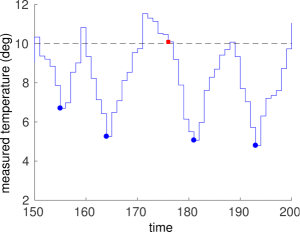
Figure 3: Simulation of $\mathit{Sys}[\delta\leftarrow\frac{19}{20}]$.

Everything is in place to define our metric to estimate the impact of an attack.

Definition 15 (Impact).

Let $M=E\,{\Join_{\cal S}}\,P$ be an honest and sound CPS, where $\xi_{\mathrm{w}}{}$ is the uncertainty of $E$. We say that an attack $A$ has definitive impact $\xi$ on the system $M$ if

$$\xi=\inf\big{\{}\xi^{\prime}:\xi^{\prime}\in\mathbb{R}^{\hat{\cal X}}\>\wedge\>\xi^{\prime}{>}0\>\wedge\>M\parallel A\sqsubseteq{M[\xi_{\mathrm{w}}{}\leftarrow{\xi_{\mathrm{w}}{}}{+}{\xi^{\prime}}]}\big{\}}.$$

It has pointwise impact $\xi$ on the system $M$ at time $m$ if

$$\xi{=}\inf\big{\{}\xi^{\prime}:\xi^{\prime}{\in}\mathbb{R}^{\hat{\cal X}}\,\wedge\,M\parallel A\sqsubseteq_{m..n}M[\xi_{\mathrm{w}}{}\leftarrow{\xi_{\mathrm{w}}{}}{+}{\xi^{\prime}}],n{\in}\mathbb{N}{\cup}\infty\big{\}}.$$

Intuitively, with this definition, we can establish either the definitive (and hence maximum) impact of the attack $A$ on the system $M$, or the impact at a specific time $m$. In the latter case, by definition of $\sqsubseteq_{m..n}$, there are two possibilities: either the impact of the attack keeps growing after time $m$, or in the time interval $m{+}1$, the system under attack deadlocks.

The impact of $\mathit{Top}(C)$ provides an upper bound for the impact of all attacks of class $C^{\prime}$, with $C^{\prime}\preceq C$.

Theorem 2 (Top attacker’s impact).

Let $M$ be an honest and sound CPS, and $C$ an arbitrary class of attacks. Let $A$ be an attack of class $C^{\prime}$, with $C^{\prime}\preceq C$.

• The definitive impact of $\mathit{Top}(C)$ on $M$ is greater than or equal to the definitive impact of $A$ on $M$.

• If $\mathit{Top}(C)$ has pointwise impact $\xi$ on $M$ at time $m$, and $A$ has pointwise impact $\xi^{\prime}$ on $M$ at time $m^{\prime}$, with $m^{\prime}\leq m$, then $\xi^{\prime}\leq\xi$.

Example 7.

Let us consider the attack $A$ of Example 4. Then, $A$ has a definitive impact of $8.5$ on the CPS $\mathit{Sys}$ defined in Example 2. Formally, $8.5=\inf\big{\{}\,\xi^{\prime}:\>\xi^{\prime}>0\>\wedge\>\mathit{Sys}\parallel A\,\sqsubseteq\,\mathit{Sys}[\delta\leftarrow\delta{+}\xi^{\prime}]\big{\}}.$ Here, the attack can prevent the activation of the cooling system, and the temperature will keep growing until the CPS before enters continuously in an unsafe state and eventually deadlocks. Since $\delta+\xi=0.4+8.5=8.9$, the proof of this statement relies on the following proposition.

Proposition 9.

Let $\mathit{Sys}$ be the CPS defined in Example 2, and $A$ be the attack defined in Example 7. Then:

• $\mathit{Sys}\parallel A\,\not\sqsubseteq\,\mathit{Sys}[\delta\leftarrow\gamma]$, for $\gamma\in(0.4,8.9)$,

• $\mathit{Sys}\parallel A\,\sqsubseteq\,\mathit{Sys}[\delta\leftarrow\gamma]$, for $\gamma>8.9$.

Definition 15 provided an instrument to estimate the impact of a successful attack. However, there is at least another question that a CPS designer could ask: “Is there a way to estimate the chances that an attack will be successful during the execution of my CPS?” To paraphrase in a more operational manner: how many execution traces of my CPS are prone to be attacked by a specific attack?

For instance, consider again the simple attack $A_{m}$ proposed in Example 3:

$$\mathsf{idle}^{m{-}1}.\mathsf{timeout}\lfloor\mathsf{read}\,\mbox{\Lightning}cool(x).\mathsf{if}\,(x{=}{\mathsf{off}})\,{\{\mathsf{write}\,\mbox{\Lightning}cool\langle\mathsf{off}\rangle}\}\rfloor.$$

Here, in the $m$-th time slot the attack tries to eavesdrop a command to turn on the cooling. The attack is very quick and condensed in a single time slot. The question is: what are the chances of success of such a quick attack?

Figure 4: A quantitative analysis of the attack of Example 3.

Figure 4 provides a representation of an experiment in MATLAB where we launched $10000$ executions of our CPS in isolation, lasting $700$ time units each. From the aggregated data contained in this graphic, we note that after a transitory phase (whose length depends on several things: the uncertainty $\delta$, the initial state of the system, the length of the cooling activity, etc.) that lasts around $300$ time slots, the rate of success of the attack $A_{m}$ is around $10\%$. The reader may wonder why exactly the $10\%$. This depends on the periodicity of our CPS, as in average the cooling is activated every $10$ time slots.

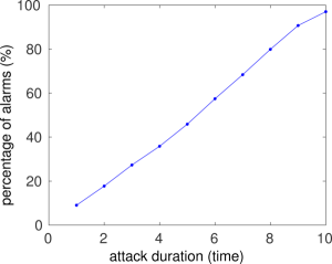
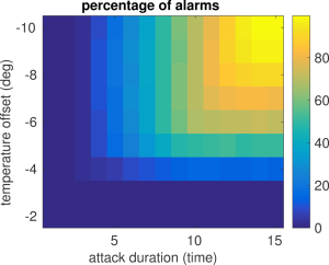
Figure 5: A quantitative analysis of two different attacks.

This example shows that, as pointed out in [8], the effectiveness of a cyber-physical attack depends on the information the attack has about the functionality of the whole CPS. For instance, if the attacker were not aware of the exact periodicity of the CPS, she might try, if possible, to repeat the attack on more consecutive time slots. In this case, the left graphic of Figure 5 says that the rate of success of the attack increases linearly with the length of the attack itself (data obtained by attacking the CPS after the transitory period). Thus, if the attack of Example 3 were iterated for $10$ time slots, say

$$\begin{array}[]{rcl}A^{10}_{m}&=&\mathsf{idle}^{m{-}1}.B_{10}\\[1.0pt] B_{i}&=&\mathsf{timeout}\lfloor{\mathsf{read}\,\mbox{\Lightning}cool(x)}.\mathsf{if}\,(x={\mathsf{off}})\\ &&\{{\mathsf{write}\,\mbox{\Lightning}cool\langle\mathsf{off}\rangle}.\mathsf{idle}.B_{i-1}\}\rfloor{B_{i-1}},\mbox{\small$\textrm{ for }1\leq i\leq 10$}\end{array}$$

with $B_{0}=\mathsf{nil}$, the rate of success would be almost $100\%$.

Finally, consider a generalisation of the attack of Example 5:

$$\begin{array}[]{rcl}A_{0}^{k}&=&\mathsf{nil}\\[1.0pt] A^{k}_{n}&=&\mathsf{timeout}\lfloor\mathsf{read}\,\mbox{\Lightning}s_{\mathrm{t}}(x).\mathsf{timeout}\lfloor\mathsf{write}\,\mbox{\Lightning}s_{\mathrm{t}}\langle x{-}k\rangle.\\ &&\mathsf{idle}.A_{n-1}^{k}\rfloor{A_{n-1}^{k}}\rfloor{A_{n-1}^{k}}\end{array}$$

for $1\leq n\leq 15$ and $2\leq k\leq 10$. Here, the attack decreases the sensed temperature of an offset $k$. Now, suppose to launch this attack after, say, $300$ time slots (i.e., after the transitory phase). Formally, we define the attack: $B^{k}_{n}\;=\;\mathsf{idle}^{300}.A_{n}^{k}$. In this case, the right graphic of Figure 5 provides a graphical representation of the percentage of alarms on $5000$ execution traces lasting $100$ time units each. Thus, for instance, an attack lasting $n=8$ time units with an offset $k=5$ affects around $40\%$ of the execution traces of the CPS.

V Conclusions, related and future work

We have provided formal theoretical foundations to reason about and statically detect attacks to physical devices of CPSs. To that end, we have proposed a hybrid process calculus, called CCPSA, as a formal specification language to model physical and cyber components of CPSs as well as cyber-physical attacks. Based on CCPSA and its labelled transition semantics, we have formalised a threat model for CPSs by grouping attacks in classes, according to the target physical devices and two timing parameters: begin and duration of the attacks. Then, we relied on the trace semantics of CCPSA to assess attack tolerance/vulnerability with respect to a given attack. Along the lines of GNDC [6], we defined a notion of top attacker, $\mathit{Top}(C)$, of a given class of attacks $C$, which has been used to provide sufficient criteria to prove attack tolerance/vulnerability to all attacks of class $C$ (and weaker ones). Here, would like to mention that in our companion paper [2] we developed a bisimulation congruence for a simpler version of the calculus where security features have been completely stripped off. For simplicity, in the current submission, we adopted as main behavioural equivalence trace equivalence instead of bisimulation. We could switch to a bisimulation semantics, preserved by parallel composition, which would allow us to scale our verification method (Theorem 1) to bigger systems. Finally, we have provided a metric to estimate the impact of a successful attack on a CPS together with possible quantifications of the success chances of an attack. We proved that the impact of the most powerful attack $\mathit{Top}(C)$ represents an upper bound for the impact of any attack $A$ of class $C$ (and weaker ones).

We have illustrated our concepts by means of a running example, focusing in particular on a formal treatment of both integrity and DoS attacks to sensors and actuators of CPSs. Our example is simple but far from trivial and designed to describe a wide number of attacks.

Related work

Among the $118$ papers discussed in the comprehensive survey [24], $50$ adopt a discrete notion of time similar to ours, $13$ a continuous one, $48$ a quasi-static time model, and the rest use a hybrid time model. Most of these papers investigate attacks on CPSs and their protection by relying on simulation test systems to validate the results.

We focus on the papers that are most related to our work. Huang et al. [10] were among the first to propose threat models for CPSs. Along with [11, 12], they stressed the role played by timing parameters on integrity and DoS attacks. Alternative threat models are discussed in [7, 8, 19]. In particular, Gollmann et al. [8] discussed possible goals (equipment damage, production damage, compliance violation) and stages (access, discovery, control, damage, cleanup) of cyber-physical attacks. In the current paper, we focused on the damage stage, where the attacker already has a rough idea of the plant and the control architecture of the target CPS.

A number of works use formal methods for CPS security, although they apply methods, and most of the time have goals, that are quite different from ours.

Burmester et al. [3] employed hybrid timed automata to give a threat framework based on the traditional Byzantine faults model for crypto-security. However, as remarked in [19], cyber-physical attacks and faults have inherently distinct characteristics. Faults are considered as physical events that affect the system behaviour, where simultaneous events don’t act in a coordinated way; cyber-attacks may be performed over a significant number of attack points and in a coordinated way.

In [21], Vigo presented an attack scenario that addresses some of the peculiarities of a cyber-physical adversary, and discussed how this scenario relates to other attack models popular in the security protocol literature. Then, in [22, 23] Vigo et al. proposed an untimed calculus of broadcasting processes equipped with notions of failed and unwanted communication. These works differ quite considerably from ours, e.g., they focus on DoS attacks without taking into consideration timing aspects or impact of the attack.

Cómbita et al. [4] and Zhu and Basar [25] applied game theory to capture the conflict of goals between an attacker who seeks to maximise the damage inflicted to a CPS’s security and a defender who aims to minimise it [13].

Finally, there are three recent papers that were developed in parallel to ours: [14, 16, 17]. Rocchetto and Tippenhaur [16] introduced a taxonomy of the diverse attacker models proposed for CPS security and outline requirements for generalised attacker models; in [17], they then proposed an extended Dolev-Yao attacker model suitable for CPSs. In their approach, physical layer interactions are modelled as abstract interactions between logical components to support reasoning on the physical-layer security of CPSs. This is done by introducing additional orthogonal channels. Time is not represented.

Nigam et al. [14] work around the notion of Timed Dolev-Yao Intruder Models for Cyber-Physical Security Protocols by bounding the number of intruders required for the automated verification of such protocols. Following a tradition in security protocol analysis, they provide an answer to the question: How many intruders are enough for verification and where should they be placed? They also extend the strand space model to CPS protocols by allowing for the symbolic representation of time, so that they can use the tool Maude [15] along with SMT support. Their notion of time is however different from ours, as they focus on the time a message needs to travel from an agent to another. The paper does not mention physical devices, such as sensors and/or actuators.

Future work

While much is still to be done, we believe that our paper provides a stepping stone for the development of formal and automated tools to analyse the security of CPSs. We will consider applying, possibly after proper enhancements, existing tools and frameworks for automated security protocol analysis, resorting to the development of a dedicated tool if existing ones prove not up to the task. We will also consider further security properties and concrete examples of CPSs, as well as other kinds of cyber-physical attackers and attacks, e.g., periodic attacks. This will allow us to refine the classes of attacks we have given here (e.g., by formalising a type system amenable to static analysis), and provide a formal definition of when a CPS is more secure than another so as to be able to design, by progressive refinement, secure variants of a vulnerable CPSs.

We also aim to extend the preliminary quantitative analysis we have given here by developing a suitable behavioural theory ensuring that our trace semantics considers also the probability of a trace to actually occur. We expect that the discrete time stochastic hybrid systems of [1] will be useful to that extent.

Appendix A Proofs

A-A Proof of § II

In order to prove Proposition 2 and Proposition 3, we use the following lemma that formalises the invariant properties binding the state variable $\mathit{temp}$ with the activity of the cooling system.

Intuitively, when the cooling system is inactive the value of the state variable $\mathit{temp}$ lays in the real interval $[0,11.5]$. Furthermore, if the coolant is not active and the variable $\mathit{temp}$ lays in the real interval $(10.1,11.5]$, then the cooling will be turned on in the next time slot. Finally, when active the cooling system will remain so for $k\in 1..5$ time slots (counting also the current time slot) with the variable $\mathit{temp}$ being in the real interval $(9.9-k{*}(1{+}\delta),11.5-k{*}(1{-}\delta)]$.

Lemma 1.

Let $\mathit{Sys}$ be the system defined in Example 2. Let

$$\mathit{Sys}=\mathit{Sys_{1}}\mathrel{\;\raisebox{0.0pt}{$\stackrel{{\scriptstyle\,t_{1}}}{{\makebox[10.97507pt]{\rule{0.0pt}{3.87498pt}\mbox{}\leavevmode\xleaders\hbox{$\mkern-2.6mu\relbar\mkern-2.6mu$}\hfill\mbox{}}}}$}\rightarrow}\mathrel{\;\raisebox{0.0pt}{$\stackrel{{\scriptstyle\,\mathsf{idle}}}{{\makebox[16.70006pt]{\rule{0.0pt}{3.87498pt}\mbox{}\leavevmode\xleaders\hbox{$\mkern-2.6mu\relbar\mkern-2.6mu$}\hfill\mbox{}}}}$}\rightarrow}\mathit{Sys_{2}}\mathrel{\;\raisebox{0.0pt}{$\stackrel{{\scriptstyle\,t_{2}}}{{\makebox[10.97507pt]{\rule{0.0pt}{3.87498pt}\mbox{}\leavevmode\xleaders\hbox{$\mkern-2.6mu\relbar\mkern-2.6mu$}\hfill\mbox{}}}}$}\rightarrow}\mathrel{\;\raisebox{0.0pt}{$\stackrel{{\scriptstyle\,\mathsf{idle}}}{{\makebox[16.70006pt]{\rule{0.0pt}{3.87498pt}\mbox{}\leavevmode\xleaders\hbox{$\mkern-2.6mu\relbar\mkern-2.6mu$}\hfill\mbox{}}}}$}\rightarrow}\dots\mathrel{\;\raisebox{0.0pt}{$\stackrel{{\scriptstyle\,t_{n-1}}}{{\makebox[14.3359pt]{\rule{0.0pt}{3.87498pt}\mbox{}\leavevmode\xleaders\hbox{$\mkern-2.6mu\relbar\mkern-2.6mu$}\hfill\mbox{}}}}$}\rightarrow}\mathrel{\;\raisebox{0.0pt}{$\stackrel{{\scriptstyle\,\mathsf{idle}}}{{\makebox[16.70006pt]{\rule{0.0pt}{3.87498pt}\mbox{}\leavevmode\xleaders\hbox{$\mkern-2.6mu\relbar\mkern-2.6mu$}\hfill\mbox{}}}}$}\rightarrow}\mathit{Sys_{n}}$$

such that the traces $t_{j}$ contain no $\mathsf{idle}$-actions, for any $j\in 1..n{-}1$, and for any $i\in 1..n$, $\mathit{Sys_{i}}=E_{i}\,{\Join}\,P_{i}$ with $E_{i}=\langle\xi_{\mathrm{x}}^{i}{},\xi_{\mathrm{u}}^{i}{},\delta,\mathit{evol}{},\epsilon,\mathit{meas}{},\mathit{inv}{}\rangle$. Then, for any $i\in 1..n{-}1$, we have the following:

1. if $\xi_{\mathrm{u}}^{i}{}(\mathit{cool})=\mathsf{off}$ then $\xi_{\mathrm{x}}^{i}{}(\mathit{temp})\in[0,11.1+\delta]$; with $\xi_{\mathrm{x}}^{i}{}(\mathit{stress})=0$ if $\xi_{\mathrm{x}}^{i}{}(\mathit{temp})\in[0,10.9+\delta]$, and $\xi_{\mathrm{x}}^{i}{}(\mathit{stress})=1$, otherwise;

2. if $\xi_{\mathrm{u}}^{i}{}(\mathit{cool})=\mathsf{off}$ and $\xi_{\mathrm{x}}^{i}{}(\mathit{temp})\in(10.1,11.1+\delta]$ then, in the next time slot, $\xi_{\mathrm{u}}^{i{+}1}{}(\mathit{cool})=\mathsf{on}$ and $\xi_{\mathrm{x}}^{i{+}1}{}(\mathit{stress})\in 1..2$;

3. if $\xi_{\mathrm{u}}^{i}{}(\mathit{cool})=\mathsf{on}$ then $\xi_{\mathrm{x}}^{i}{}(\mathit{temp})\in(9.9-k{*}(1{+}\delta),11.1+\delta-k{*}(1{-}\delta)]$, for some $k\in 1..5$ such that $\xi_{\mathrm{u}}^{i-k}{}(\mathit{cool})=\mathsf{off}$ and $\xi_{\mathrm{u}}^{i-j}{}(\mathit{cool})=\mathsf{on}$, for $j\in 0..k{-}1$; moreover, if $k\in 1..3$ then $\xi_{\mathrm{x}}^{i}{}(\mathit{stress})\in 1..k{+}1$, otherwise, $\xi_{\mathrm{x}}^{i}{}(\mathit{stress})=0$.

Proof.

Let us write $v_{i}$ and $s_{i}$ to denote the values of the state variables $\mathit{temp}$ and $\mathit{stress}$, respectively, in the systems $\mathit{Sys_{i}}$, i.e., $\xi_{\mathrm{x}}^{i}{}(\mathit{temp})=v_{i}$ and $\xi_{\mathrm{x}}^{i}{}(\mathit{stress})=s_{i}$. Moreover, we will say that the coolant is active (resp., is not active) in $\mathit{Sys_{i}}$ if $\xi_{\mathrm{u}}^{i}{}(\mathit{cool})=\mathsf{on}$ (resp., $\xi_{\mathrm{u}}^{i}{}(\mathit{cool})=\mathsf{off}$).

The proof is by mathematical induction on $n$, i.e., the number of $\mathsf{idle}$-actions of our traces.

The case base $n=1$ follows directly from the definition of $\mathit{Sys}$.

Let us prove the inductive case. We assume that the three statements hold for $n-1$ and prove that they also hold for $n$.

1. Let us assume that the cooling is not active in $\mathit{Sys_{n}}$. In this case, we prove that $v_{n}\in[0,11.1+\delta]$, with and $s_{n}=0$ if $v_{n}\in[0,10.9+\delta]$, and $s_{n}=1$ otherwise.

   We consider separately the cases in which the coolant is active or not in $\mathit{Sys_{n-1}}$

   • Suppose the coolant is not active in $\mathit{Sys_{n{-}1}}$ (and not active in $\mathit{Sys_{n}}$).

     By the induction hypothesis we have $v_{n-1}\in[0,11.1+\delta]$; with $s_{n{-}1}=0$ if $v_{n{-}1}\in[0,10.9+\delta]$, and $s_{n{-}1}=1$ otherwise. Furthermore, if $v_{n-1}\in(10.1,11.1+\delta]$, then, by the induction hypothesis, the coolant must be active in $\mathit{Sys_{n}}$. Since we know that in $\mathit{Sys_{n}}$ the cooling is not active, it follows that $v_{n-1}\in[0,10.1]$ and $s_{n}=0$. Furthermore, in $\mathit{Sys_{n}}$ the temperature will increase of a value laying in the real interval $[1-\delta,1+\delta]=[0.6,1.4]$. Thus, $v_{n}$ will be in $[0.6,11.1+\delta]\subseteq[0,11.1+\delta]$. Moreover, if $v_{n-1}\in[0,9.9]$, then the state variable $\mathit{stress}$ is not incremented and hence $s_{n}=0$ with $v_{n}\in[0+1-\delta\,,\,9.9+1+\delta]=[0.6\,,\,10.9+\delta]\subseteq[0\,,\,10.9+\delta]$. Otherwise, if $v_{n-1}\in(9.9,10.1]$, then the state variable $\mathit{stress}$ is incremented, and hence $s_{n}=1$.

   • Suppose the coolant is active in $\mathit{Sys_{n{-}1}}$ (and not active in $\mathit{Sys_{n}}$).

     By the induction hypothesis, $v_{n-1}\in(9.9-k*(1+\delta),11.1+\delta-k*(1-\delta)]$ for some $k\in 1..5$ such that the coolant is not active in $\mathit{Sys_{n{-}1{-}k}}$ and is active in $\mathit{Sys_{n{-}k}},\ldots,\mathit{Sys_{n-1}}$.

     The case $k\in\{1,\ldots,4\}$ is not admissible. In fact if $k\in\{1,\ldots,4\}$ then the coolant would be active for less than $5$ $\mathsf{idle}$-actions as we know that $\mathit{Sys_{n}}$ is not active. Hence, it must be $k=5$. Since $\delta=0.4$ and $k=5$, it holds that $v_{n-1}\in(9.9-5*1.4,11.1+0.4-5*0.6]=(2.8,8.6]$ and $s_{n{-}1}=0$. Moreover, since the coolant is active for $5$ time slots, in $\mathit{Sys_{n{-}1}}$ the controller and the $\mathit{IDS}$ synchronise together via channel $\mathit{sync}$ and hence the $\mathit{IDS}$ checks the temperature. Since $v_{n-1}\in(2.8,8.6]$ the $\mathit{IDS}$ process sends to the controller a command to $\mathsf{stop}$ the cooling, and the controller will switch off the cooling system. Thus, in the next time slot, the temperature will increase of a value laying in the real interval $[1-\delta,1+\delta]=[0.6,1.4]$. As a consequence, in $\mathit{Sys_{n}}$ we will have $v_{n}\in[2.8+0,6,8.6+1.4]=[3.4,10]\subseteq[0,11.1+\delta]$. Moreover, since $v_{n-1}\in(2.8,8.6]$ and $s_{n{-}1}=0$, we derive that the state variable $\mathit{stress}$ is not increased and hence $s_{n}=0$, with $v_{n}\in[3.4,10]\subseteq[0,10.9+\delta]$.

2. Let us assume that the coolant is not active in $\mathit{Sys_{n}}$ and $v_{n}\in(10.1,11.1+\delta]$; we prove that the coolant is active in $\mathit{Sys_{n{+}1}}$ with $s_{n{+}1}\in 1..2$. Since the coolant is not active in $\mathit{Sys_{n}}$, then it will check the temperature before the next time slot. Since $v_{n}\in(10.1,11.1+\delta]$ and $\epsilon=0.1$, then the process $\mathit{Ctrl}$ will sense a temperature greater than $10$ and the coolant will be turned on. Thus, the coolant will be active in $\mathit{Sys_{n{+}1}}$. Moreover, since $v_{n}\in(10.1,11.1+\delta]$, and $s_{n}$ could be either $0$ or $1$, the state variable $\mathit{stress}$ is increased and therefore $s_{n{+}1}\in 1..2$.

3. Let us assume that the coolant is active in $\mathit{Sys_{n}}$; we prove that $v_{n}\in(9.9-k*(1+\delta),11.1+\delta-k*(1-\delta)]$ for some $k\in 1..5$ and the coolant is not active in $\mathit{Sys_{n{-}k}}$ and active in $\mathit{Sys_{n-k+1}},\dots,\mathit{Sys_{n}}$. Moreover, we have to prove that if $k\leq 3$ then $s_{n}\in 1..k{+}1$, otherwise, if $k>3$ then $s_{n}=0$.

   We prove the first statement. That is, we prove that $v_{n}\in(9.9-k*(1+\delta),11.1+\delta-k*(1-\delta)]$, for some $k\in 1..5$, and the coolant is not active in $\mathit{Sys_{n{-}k}}$, whereas it is active in the systems $\mathit{Sys_{n-k+1}},\dots,\mathit{Sys_{n}}$.

   We separate the case in which the coolant is active in $\mathit{Sys_{n{-}1}}$ from that in which is not active.

   • Suppose the coolant is not active in $\mathit{Sys_{n{-}1}}$ (and active in $\mathit{Sys_{n}}$).

     In this case $k=1$ as the coolant is not active in $\mathit{Sys_{n-1}}$ and it is active in $\mathit{Sys_{n}}$. Since $k=1$, we have to prove $v_{n}\in(9.9-(1+\delta),11.1+\delta-(1-\delta)]$.

     However, since the coolant is not active in $\mathit{Sys_{n-1}}$ and is active in $\mathit{Sys_{n}}$ it means that the coolant has been switched on in $\mathit{Sys_{n-1}}$ because the sensed temperature was above $10$ (since $\epsilon=0.1$ this may happen only if $v_{n-1}>9.9$). By the induction hypothesis, since the coolant is not active in $\mathit{Sys_{n-1}}$, we have that $v_{n-1}\in[0,11.1+\delta]$. Therefore, from $v_{n-1}>9.9$ and $v_{n-1}\in[0,11.1+\delta]$ it follows that $v_{n-1}\in(9.9,11.1+\delta]$. Furthermore, since the coolant is active in $\mathit{Sys_{n}}$, the temperature will decrease of a value in $[1-\delta,1+\delta]$ and therefore $v_{n}\in(9.9-(1+\delta),11.1+\delta-(1-\delta)]$, which concludes this case of the proof.

   • Suppose the coolant is active in $\mathit{Sys_{n{-}1}}$ (and active in $\mathit{Sys_{n}}$ as well).

     By the induction hypothesis, there is $h\in 1..5$ such that $v_{n-1}\in(9.9-h*(1+\delta),11.1+\delta-h*(1-\delta)]$ and the coolant is not active in $\mathit{Sys_{n{-}1{-}h}}$ and is active in $\mathit{Sys_{n{-}h}},\ldots,\mathit{Sys_{n{-}1}}$.

     The case $h=5$ is not admissible. In fact, since $\delta=0.4$, if $h=5$ then $v_{n-1}\in(9.9-5*1.4,11.1+\delta-5*0.6]=(2.8,8.6]$. Furthermore, since the cooling system has been active for $5$ time instants, in $\mathit{Sys_{n{-}1}}$ the controller and the IDS synchronise together via channel $\mathit{sync}$, and the $\mathit{IDS}$ checks the received temperature. As $v_{n-1}\in(2.8,8.6]$, the $\mathit{IDS}$ sends to the controller via channel $\mathit{ins}$ the command $\mathsf{stop}$. This implies that the controller should turn off the cooling system, in contradiction with the hypothesis that the coolant is active in $\mathit{Sys_{n}}$.

     Hence, it must be $h\in 1..4$. Let us prove that for $k=h+1$ we obtain our result. Namely, we have to prove that, for $k=h+1$, (i) $v_{n}\in(9.9-k*(1+\delta),11.1+\delta-k*(1-\delta)]$, and (ii) the coolant is not active in $\mathit{Sys_{n{-}k}}$ and active in $\mathit{Sys_{n-k+1}},\dots,\mathit{Sys_{n}}$.

     Let us prove the statement (i). By the induction hypothesis, it holds that $v_{n-1}\in(9.9-h*(1+\delta),11.1+\delta-h*(1-\delta)]$. Since the coolant is active in $\mathit{Sys_{n}}$, the temperature will decrease Hence, $v_{n}\in(9.9-(h+1)*(1+\delta),11.1+\delta-(h+1)*(1-\delta)]$. Therefore, since $k=h+1$, we have that $v_{n}\in(9.9-k*(1+\delta),11.1+\delta-k*(1-\delta)]$.

     Let us prove the statement (ii). By the induction hypothesis the coolant is not active in $\mathit{Sys_{n-1-h}}$ and it is active in $\mathit{Sys_{n-h}},\ldots,\mathit{Sys_{n-1}}$. Now, since the coolant is active in $\mathit{Sys_{n}}$, for $k=h+1$, we have that the coolant is not active in $\mathit{Sys_{n-k}}$ and is active in $\mathit{Sys_{n-k+1}},\ldots,\mathit{Sys_{n}}$, which concludes this case of the proof.

   Thus, we have proved that $v_{n}\in(9.9-k*(1+\delta),11.1+\delta-k*(1-\delta)]$, for some $k\in 1..5$; moreover, the coolant is not active in $\mathit{Sys_{n{-}k}}$ and active in the systems $\mathit{Sys_{n-k+1}},\dots,\mathit{Sys_{n}}$.

   It remains to prove that $s_{n}\in 1..k{+}1$ if $k\leq 3$, and $s_{n}=0$, otherwise.

   By inductive hypothesis, since the coolant is not active in $\mathit{Sys_{n{-}k}}$, we have that $s_{n{-}k}\in 0..1$. Now, for $k\in[1..2]$, the temperature could be greater than $9.9$. Hence if the state variable $\mathit{stress}$ is either increased or reset, then $s_{n}\in 1..k{+}1$, for $k\in 1..3$. Moreover, since for $k\in 3..5$ the temperature is below $9.9$, it follows that $s_{n}=0$ for $k>3$.

∎

Proof of Proposition 2.

Since $\delta=0.4$, by Lemma 1 the value of the state variable $\mathit{temp}$ is always in the real interval $[0,11.5]$. As a consequence, the invariant of the system is never violated and the system never deadlocks. Moreover, after $5$ time units of cooling, the state variable $\mathit{temp}$ is always in the real interval $(9.9-5*1.4,11.1+0.4-5*0.6]=(2.9,8.5]$. Hence, the process $\mathit{IDS}$ will never transmit on the channel $\mathit{alarm}$.

Finally, by Lemma 1 the maximum value reached by the state variable $\mathit{stress}$ is $4$ and therefore the system does not reach unsafe states. ∎

Proof of Proposition 3.

Let us prove the two statements separately.

• Since $\epsilon=0.1$, if process $\mathit{Ctrl}$ senses a temperature above $10$ (and hence $\mathit{Sys}$ turns on the cooling) then the value of the state variable $\mathit{temp}$ is greater than $9.9$. By Lemma 1, the value of the state variable $\mathit{temp}$ is always less than or equal to $11.1+\delta$. Therefore, if $\mathit{Ctrl}$ senses a temperature above $10$, then the value of the state variable $\mathit{temp}$ is in $(9.9,11.1+\delta]$.

• By Lemma 1 (third item), the coolant can be active for no more than $5$ time slots. Hence, by Lemma 1, when $\mathit{Sys}$ turns off the cooling system the state variable $\mathit{temp}$ ranges over $(9.9-5*(1+\delta),11.1+\delta-5*(1-\delta)]$.

∎

A-B Proofs of § III

Proof of Proposition 4.

We distinguish the two cases, depending on $m$.

• Let $m\leq 8$. We recall that the cooling system is activated only when the sensed temperature is above $10$. Since $\epsilon=0.1$, when this happens the state variable $\mathit{temp}$ must be at least $9.9$. Note that after $m{-}1\leq 7$ $\mathsf{idle}$-actions, when the attack tries to interact with the controller of the actuator $\mathit{cool}$, the variable $\mathit{temp}$ may reach at most $7*(1+\delta)=7*1.4=9.8$ degrees. Thus, the cooling system will not be activated and the attack will not have any effect.

• Let $m>8$. By Proposition 2, the system $\mathit{Sys}$ in isolation may never deadlock, it does not get into an unsafe state, and it may never emit an output on channel $\mathit{alarm}$. Thus, any execution trace of the system $\mathit{Sys}$ consists of a sequence of $\tau$-actions and $\mathsf{idle}$-actions.

  In order to prove the statement it is enough to show the following four facts:

  • the system $\mathit{Sys}\parallel A_{m}$ may not deadlock in the first $m+3$ time slots;

  • the system $\mathit{Sys}\parallel A_{m}$ may not emit any output in the first $m+3$ time slots;

  • the system $\mathit{Sys}\parallel A_{m}$ may not enter in an unsafe state in the first $m+3$ time slots;

  • the system $\mathit{Sys}\parallel A_{m}$ has a trace reaching un unsafe state from the $(m{+}4)$-th time slot on, and until the invariant gets violated and the system deadlocks.

  The first three facts are easy to show as the attack may steal the command addressed to the actuator $\mathit{cool}$ only in the $m$-th time slot. Thus, until time slot $m$, the whole system behaves correctly. In particular, by Proposition 2 and Proposition 3, no alarms, deadlocks or violations of safety conditions occur, and the temperature lies in the expected ranges. Any of those three actions requires at least further $4$ time slots to occur. Indeed, by Lemma 1, when the cooling is switched on in the time slot $m$, the variable $\mathit{stress}$ might be equal to $2$ and hence the system might not enters in an unsafe state in the first $m+3$ time slots. Moreover, an alarm or a deadlock needs more than $3$ time slots and hence no alarm can occur in the first $m+3$ time slots.

  Let us show the fourth fact, i.e., that there is a trace where the system $\mathit{Sys}\parallel A_{m}$ enters into an unsafe state starting from the $(m{+}4)$-th time slot and until the invariant gets violated.

  Firstly, we prove that for all time slots $n$, with $9\leq n<m$, there is a trace of the system $\mathit{Sys}\parallel A_{m}$ in which the state variable $\mathit{temp}$ reaches the values $10.1$ in the time slot $n$.

  The fastest trace reaching the temperature of $10.1$ degrees requires $\lceil\frac{10.1}{1+\delta}\rceil=\lceil\frac{10.1}{1.4}\rceil=8$ time units, whereas the slowest one $\lceil\frac{10.1}{1-\delta}\rceil=\lceil\frac{10.1}{0.6}\rceil=17$ time units. Thus, for any time slot $n$, with $9\leq n\leq 18$, there is a trace of the system where the value of the state variable $\mathit{temp}$ is $10.1$. Now, for any of those time slots $n$ there is a trace in which the state variable $\mathit{temp}$ is equal to $10.1$ in all time slots $n+10i<m$, with $i\in\mathbb{N}$. Indeed, when the variable $\mathit{temp}$ is equal to $10.1$ the cooling might be activated. Thus, there is a trace in which the cooling system is activated. We can always assume that during the cooling the temperature decreases of $1+\delta$ degrees per time unit, reaching at the end of the cooling cycle the value of $5$. This entails that the trace may continue with $5$ time slots in which the variable $\mathit{temp}$ is increased of $1+\delta$ degrees per time unit; reaching again the value $10.1$. Thus, for all time slots $n$, with $9\leq n<m$, there is a trace of the system $\mathit{Sys}\parallel A_{m}$ in which the state variable $\mathit{temp}$ is $10.1$ in $n$.

  As a consequence, we can suppose that in the $m{-}1$-th time slot there is a trace in which the value of the variable $\mathit{temp}$ is $10.1$. Since $\epsilon=0.1$, the sensed temperature lays in the real interval $[10,10.2]$. Let us focus on the trace in which the sensed temperature is $10$ and the cooling system is not activated. In this case, in the $m$-th time slot the system may reach a temperature of $10.1+(1+\delta)=11.5$ degrees and the variable $\mathit{stress}$ is $1$.

  The process $\mathit{Ctrl}$ will sense a temperature above $10$ sending the command $cool!\mathsf{on}$ to the actuator $\mathit{cool}$. Now, since the attack $A_{m}$ is active in that time slot ($m>8$), the command will be stolen by the attack and it will never reach the actuator. Without that dose of coolant, the temperature of the system will continue to grow. As a consequence, after further $4$ time units of cooling, i.e. in the $m{+}4$-th time slot, the value of the state variable $\mathit{stress}$ may be $5$ and the system enters in an unsafe state.

  After $1$ time slots, in the time slot $m+5$, the controller and the $\mathit{IDS}$ synchronise via channel $\mathit{sync}$, the $\mathit{IDS}$ will detect a temperature above $10$, and it will fire the output on channel $\mathit{alarm}$ saying to process $\mathit{Ctrl}$ to keep cooling. But $\mathit{Ctrl}$ will not send again the command $cool!\mathsf{on}$. Hence, the temperature would continue to increase and the system remains in an unsafe state while the process $\mathit{IDS}$ will keep sending of $\mathit{alarm}$(s) until the invariant of the environment gets violated.

∎

Proof of Proposition 5.

By induction on the length of the trace. ∎

In order to prove Proposition 6, we introduce Lemma 2. This is a variant of Lemma 1 in which the CPS $\mathit{Sys}$ runs in parallel with the attack $A_{n}$ defined in Example 5. Here, due to the presence of the attack, the temperature is $2$ degrees higher when compared to the system $\mathit{Sys}$ in isolation.

Lemma 2.

Let $\mathit{Sys}$ be the system defined in Example 2 and $A_{n}$ be the attack of Example 5. Let

$$\mathit{Sys}\parallel A_{n}=\mathit{Sys_{1}}\mathrel{\;\raisebox{0.0pt}{$\stackrel{{\scriptstyle\,t_{1}}}{{\makebox[10.97507pt]{\rule{0.0pt}{3.87498pt}\mbox{}\leavevmode\xleaders\hbox{$\mkern-2.6mu\relbar\mkern-2.6mu$}\hfill\mbox{}}}}$}\rightarrow}\mathrel{\;\raisebox{0.0pt}{$\stackrel{{\scriptstyle\,\mathsf{idle}}}{{\makebox[16.70006pt]{\rule{0.0pt}{3.87498pt}\mbox{}\leavevmode\xleaders\hbox{$\mkern-2.6mu\relbar\mkern-2.6mu$}\hfill\mbox{}}}}$}\rightarrow}\dots\mathit{Sys_{n-1}}\mathrel{\;\raisebox{0.0pt}{$\stackrel{{\scriptstyle\,t_{n-1}}}{{\makebox[14.3359pt]{\rule{0.0pt}{3.87498pt}\mbox{}\leavevmode\xleaders\hbox{$\mkern-2.6mu\relbar\mkern-2.6mu$}\hfill\mbox{}}}}$}\rightarrow}\mathrel{\;\raisebox{0.0pt}{$\stackrel{{\scriptstyle\,\mathsf{idle}}}{{\makebox[16.70006pt]{\rule{0.0pt}{3.87498pt}\mbox{}\leavevmode\xleaders\hbox{$\mkern-2.6mu\relbar\mkern-2.6mu$}\hfill\mbox{}}}}$}\rightarrow}\mathit{Sys_{n}}$$

such that the traces $t_{j}$ contain no $\mathsf{idle}$-actions, for any $j\in 1..n{-}1$, and for any $i\in 1..n$ $\mathit{Sys_{i}}=E_{i}\,{\Join}\,P_{i}$ with $E_{i}=\langle\xi_{\mathrm{x}}^{i}{},\xi_{\mathrm{u}}^{i}{},\delta,\mathit{evol}{},\epsilon,\mathit{meas}{},\mathit{inv}{}\rangle$. Then, for any $i\in 1..n{-}1$ we have the following:

• if $\xi_{\mathrm{u}}^{i}{}(\mathit{cool})=\mathsf{off}$, then $\xi_{\mathrm{x}}^{i}{}(\mathit{temp})\in[0,11.1+2+\delta]$;

• if $\xi_{\mathrm{u}}^{i}{}(\mathit{cool})=\mathsf{off}$ and $\xi_{\mathrm{x}}^{i}{}(\mathit{temp})\in(10.1+2,11.1+2+\delta]$, then we have $\xi_{\mathrm{u}}^{i+1}{}(\mathit{cool})=\mathsf{on}$;

• if $\xi_{\mathrm{u}}^{i}{}(\mathit{cool})=\mathsf{on}$, then $\xi_{\mathrm{x}}^{i}{}(\mathit{temp})\in(9.9+2-k*(1+\delta),11.1+2+\delta-k*(1-\delta)]$, for some $k\in 1..5$, such that $\xi_{\mathrm{u}}^{i-k}{}(\mathit{cool})=\mathsf{off}$ and $\xi_{\mathrm{u}}^{i-j}{}(\mathit{cool})=\mathsf{on}$, for $j\in 0..k{-}1$.

Proof.

Similar to the proof of Lemma 1. ∎

Now, everything is in place to prove Proposition 6.

Proof of Proposition 6.

Let us proceed by case analysis.

• Let $0\leq n\leq 8$. In the proof of Proposition 4, we remarked that the system $\mathit{Sys}$ in isolation may sense a temperature greater than $10$ only after $8$ $\mathsf{idle}$-actions, i.e., in the $9$-th time slot. However, the life of the attack is $n\leq 8$, and in the $9$-th time slot the attack is already terminated. As a consequence, starting from the $9$-th time slot the system will correctly sense the temperature and it will correctly activate the cooling system.

• Let $n=9$. The maximum value that may be reached by the state variable $\mathit{temp}$ after $8$ $\mathsf{idle}$-actions, i.e., in the $9$-th time slot, is $8*(1+\delta)=8*1.4=11.2$. However, since in the $9$-th time slot the attack is still alive, the process $\mathit{Ctrl}$ will sense a temperature below $10$ and the system will move to the next time slot and the state variable $\mathit{stress}$ is incremented. Then, in the $10$-th time slot, when the attack is already terminated, the maximum temperature the system may reach is $11.2+(1+\delta)=12.6$ degrees and the state variable $\mathit{stress}$ is equal to $1$. Thus, the process $\mathit{Ctrl}$ will sense a temperature greater than $10$, activating the cooling system and incrementing the state variable $\mathit{stress}$. As a consequence, during the following $4$ time units of cooling, the value of the state variable $\mathit{temp}$ will be at most $12.6-4*(1-\delta)=12.6-4*0.6=10.2$, and hence in the $14$-th time slot, the value of the state variable $\mathit{stress}$ is $5$. As a consequence, the system will enter in an unsafe state. In the $15$-th time slot, the value of the state variable $\mathit{stress}$ is still equal to $5$ and the system will still be in an unsafe state. However, the value of the state variable $\mathit{temp}$ will be at most $12.6-5*(1-\delta)=12.6-5*0.6=9.6$ which will be sensed by process $\mathit{IDS}$ as at most $9.7$ (sensor error $\epsilon=0.1$). As a consequence, no alarm will be turned on and the variable $\mathit{stress}$ will be reset. Moreover, the invariant will be obviously always preserved.

  As in the current time slot the attack has already terminated, from this point in time on, the system will behave correctly with neither deadlocks or alarms.

• Let $n\geq 10$. In order to prove that $\mathit{Sys}\parallel A_{n}\,\simeq_{[14,n{+}7]}\,\mathit{Sys}$, it is enough to show that:

  • the system $\mathit{Sys}\parallel A_{n}$ does not deadlock;

  • the system $\mathit{Sys}\parallel A_{n}$ may not emit any output in the first $13$ time slots;

  • there is a trace in which the system $\mathit{Sys}\parallel A_{n}$ enters in an unsafe state in the $14$-th time slot;

  • there is a trace in which the system $\mathit{Sys}\parallel A_{n}$ is in an unsafe state in the $(n{+}7)$-th time slot;

  • the system $\mathit{Sys}\parallel A_{n}$ does not have any execution trace emitting an output along channel $\mathit{alarm}$ or entering in an unsafe state after the $n+7$-th time slot.

  As regards the first fact, since $\delta=0.4$, by Lemma 2 the temperature of the system under attack will always remain in the real interval $[0,13.5]$. Thus, the invariant is never violated and the trace of the system under attack cannot contain any $\mathsf{deadlock}$-action. Moreover, when the attack terminates, if the temperature is in $[0,9.9]$, the system will continue his behaviour correctly, as in isolation. Otherwise, since the temperature is at most $13.5$, after a possible sequence of cooling cycles, the temperature will reach a value in the interval $[0,9.9]$, and again the system will continue its behaviour correctly, as in isolation.

  Concerning the second and the third facts, the proof is analogous to that of case $n=9$.

  Concerning the fourth fact, firstly we prove that for all time slots $m$, with $9<m\leq n$, there is a trace of the system $\mathit{Sys}\parallel A_{n}$ in which the state variable $\mathit{temp}$ reaches the values $12$ in the time slot $m$. Since the attack is alive at that time, and $\epsilon=0.1$, when the variable $\mathit{temp}$ will be equal to $12$ the sensed temperature will lay in the real interval $[9.9,10.1]$.

  The fastest trace reaching the temperature of $12$ degrees requires $\lceil\frac{12}{1+\delta}\rceil=\lceil\frac{12}{1.4}\rceil=9$ time units, whereas the slowest one $\lceil\frac{12}{1-\delta}\rceil=\lceil\frac{12}{0.6}\rceil=20$ time units. Thus, for any time slot $m$, with $9<m\leq 21$, there is a trace of the system where the value of the state variable $\mathit{temp}$ is $12$. Now, for any of those time slots $m$ there is a trace in which the state variable $\mathit{temp}$ is equal to $12$ in all time slots $m+10i<n$, with $i\in\mathbb{N}$. As already said, when the variable $\mathit{temp}$ is equal to $12$ the sensed temperature lays in the real interval $[9.9,10.1]$ and the cooling might be activated. Thus, there is a trace in which the cooling system is activated. We can always find a trace where during the cooling the temperature decreases of $1+\delta$ degrees per time unit, reaching at the end of the cooling cycle the value of $5$. Thus, the trace may continue with $5$ time slots in which the variable $\mathit{temp}$ is increased of $1+\delta$ degrees per time unit; reaching again the value $12$. Thus, for all time slots $m$, with $9<m\leq n$, there is a trace of the system $\mathit{Sys}\parallel A_{n}$ in which the state variable $\mathit{temp}$ has value $12$ in the time slot $m$.

  Therefore, we can suppose that in the $n$-th time slot the variable $\mathit{temp}$ is equal to $12$ and, since the maximum increment of temperature is $1.4$, the the variable $\mathit{stress}$ is at least equal to $1$. Since the attack is alive and $\epsilon=0.1$, in the $n$-th time slot the sensed temperature will lay in $[9.9,10.1]$. We consider the case in which the sensed temperature is less than $10$ and hence the cooling is not activated.

  Thus, in the $n{+}1$-th time slot the system may reach a temperature of $12+1+\delta=13.4$ degrees and the process $\mathit{Ctrl}$ will sense a temperature above $10$, and it will activate the cooling system. In this case, the variable $\mathit{stress}$ will be increased. As a consequence, after further $5$ time units of cooling, i.e. in the $n{+}6$-th time slot, the value of the state variable $\mathit{temp}$ may reach $13.5-5*(1-\delta)=10.4$ and the alarm will be fired and the variable $\mathit{stress}$ will be still equal to $5$. Therefore, in the $n{+}7$-th time slot the variable $\mathit{stress}$ will be still equal to $5$ and the system will be in an unsafe state.

  Concerning the fifth fact, by Lemma 2, in the $n{+}1$-th time slot the attack will be terminated and the system may reach a temperature that is, in the worst case, at most $13.5$. Thus, the cooling system may be activated and the variable $\mathit{stress}$ will be increased. As a consequence, in the $n{+}7$-th time slot, the value of the state variable $\mathit{temp}$ may be at most $13.5-6*(1-\delta)=13.5-6*0.6=9.9$ and the variable $\mathit{stress}$ will be reset to $0$. Thus, after the $n+7$-th time slot, the system will behave correctly, as in isolation.

∎

In order to prove Theorem 1, we introduce the following lemma.

Lemma 3.

Let $M$ be an honest and sound CPS, $C$ a class of attacks, and $A$ an attack of an arbitrary class $C^{\prime}\preceq C$. Whenever $M\parallel A\mathrel{\;\raisebox{0.0pt}{$\stackrel{{\scriptstyle\,t}}{{\makebox[10.19447pt]{\rule{0.0pt}{4.30554pt}\mbox{}\leavevmode\xleaders\hbox{$\mkern-2.6mu\relbar\mkern-2.6mu$}\hfill\mbox{}}}}$}\rightarrow}M^{\prime}\parallel A^{\prime}$, then

$$M\parallel\mathit{Top}(C)\mathrel{\;\raisebox{0.0pt}{$\stackrel{{\scriptstyle\,t}}{{\makebox[10.19447pt]{\rule{0.0pt}{4.30554pt}\mbox{}\leavevmode\xleaders\hbox{$\mkern-2.6mu\relbar\mkern-2.6mu$}\hfill\mbox{}}}}$}\rightarrow}M^{\prime}\parallel\prod_{\iota\in\mathcal{I}}\mathit{Att}(\iota,\#\mathsf{idle}(t){+}1,C(\iota))\enspace.$$

Proof.

Let us denote with $\mathit{Top}^{h}(C)$ the attack process

$$\prod_{\iota\in\mathcal{I}}\mathit{Att}(\iota,h,C(\iota)).$$

Obviously, $\mathit{Top}^{1}(C)=\mathit{Top}(C)$.

The proof is by mathematical induction on the length $k$ of the trace $t$.

Base case $k=1$.
This means $t=\alpha$, for some action $\alpha$. We proceed by case analysis on the action $\alpha$.

• $\alpha=\overline{c}v$. Since the attacker $A$ does not use a communication channel, from $M\parallel A\mathrel{\;\raisebox{0.0pt}{$\stackrel{{\scriptstyle\,\overline{c}v}}{{\makebox[16.31091pt]{\rule{0.0pt}{4.30554pt}\mbox{}\leavevmode\xleaders\hbox{$\mkern-2.6mu\relbar\mkern-2.6mu$}\hfill\mbox{}}}}$}\rightarrow}M^{\prime}\parallel A^{\prime}$ we can derive that $A=A^{\prime}$ and $M\mathrel{\;\raisebox{0.0pt}{$\stackrel{{\scriptstyle\,\overline{c}v}}{{\makebox[16.31091pt]{\rule{0.0pt}{4.30554pt}\mbox{}\leavevmode\xleaders\hbox{$\mkern-2.6mu\relbar\mkern-2.6mu$}\hfill\mbox{}}}}$}\rightarrow}M^{\prime}$. Hence by rules (Par) and (Out), we derive $M\parallel\mathit{Top}(C)\mathrel{\;\raisebox{0.0pt}{$\stackrel{{\scriptstyle\,\overline{c}v}}{{\makebox[16.31091pt]{\rule{0.0pt}{4.30554pt}\mbox{}\leavevmode\xleaders\hbox{$\mkern-2.6mu\relbar\mkern-2.6mu$}\hfill\mbox{}}}}$}\rightarrow}M^{\prime}\parallel\mathit{Top}^{1}(C)=M^{\prime}\parallel\mathit{Top}(C)$.

• $\alpha=cv$. This case is similar to the previous one.

• $\alpha=\tau$. There are several sub-cases.

  • Let $M\parallel A\mathrel{\;\raisebox{0.0pt}{$\stackrel{{\scriptstyle\,\tau}}{{\makebox[10.72676pt]{\rule{0.0pt}{4.30554pt}\mbox{}\leavevmode\xleaders\hbox{$\mkern-2.6mu\relbar\mkern-2.6mu$}\hfill\mbox{}}}}$}\rightarrow}M^{\prime}\parallel A^{\prime}$ be derived by an application of rule (SensReadSec). Since the attacker $A$ performs only malicious actions on physical devices, from $M\parallel A\mathrel{\;\raisebox{0.0pt}{$\stackrel{{\scriptstyle\,\tau}}{{\makebox[10.72676pt]{\rule{0.0pt}{4.30554pt}\mbox{}\leavevmode\xleaders\hbox{$\mkern-2.6mu\relbar\mkern-2.6mu$}\hfill\mbox{}}}}$}\rightarrow}M^{\prime}\parallel A^{\prime}$ we can derive that $A=A^{\prime}$ and $P\mathrel{\;\raisebox{0.0pt}{$\stackrel{{\scriptstyle\,s?v}}{{\makebox[17.8977pt]{\rule{0.0pt}{4.30554pt}\mbox{}\leavevmode\xleaders\hbox{$\mkern-2.6mu\relbar\mkern-2.6mu$}\hfill\mbox{}}}}$}\rightarrow}P^{\prime}$, for some processes $P$ and $P^{\prime}$ such that $M=E\,{\Join_{\cal S}}\,P$ and $M^{\prime}=E\,{\Join_{\cal S}}\,P^{\prime}$. Hence by an application of rules (Par) and (SensReadSec) we derive $M\parallel\mathit{Top}(C)\mathrel{\;\raisebox{0.0pt}{$\stackrel{{\scriptstyle\,\tau}}{{\makebox[10.72676pt]{\rule{0.0pt}{4.30554pt}\mbox{}\leavevmode\xleaders\hbox{$\mkern-2.6mu\relbar\mkern-2.6mu$}\hfill\mbox{}}}}$}\rightarrow}M^{\prime}\parallel\mathit{Top}^{1}(C)=M^{\prime}\parallel\mathit{Top}(C)$.

  • Let $M\parallel A\mathrel{\;\raisebox{0.0pt}{$\stackrel{{\scriptstyle\,\tau}}{{\makebox[10.72676pt]{\rule{0.0pt}{4.30554pt}\mbox{}\leavevmode\xleaders\hbox{$\mkern-2.6mu\relbar\mkern-2.6mu$}\hfill\mbox{}}}}$}\rightarrow}M^{\prime}\parallel A^{\prime}$ be derived by an application of rule (ActWriteSec). This case is similar to the previous one.

  • Let $M\parallel A\mathrel{\;\raisebox{0.0pt}{$\stackrel{{\scriptstyle\,\tau}}{{\makebox[10.72676pt]{\rule{0.0pt}{4.30554pt}\mbox{}\leavevmode\xleaders\hbox{$\mkern-2.6mu\relbar\mkern-2.6mu$}\hfill\mbox{}}}}$}\rightarrow}M^{\prime}\parallel A^{\prime}$ be derived by an application of rule (SensReadUnSec). Since the attacker $A$ performs only malicious actions, from $M\parallel A\mathrel{\;\raisebox{0.0pt}{$\stackrel{{\scriptstyle\,\tau}}{{\makebox[10.72676pt]{\rule{0.0pt}{4.30554pt}\mbox{}\leavevmode\xleaders\hbox{$\mkern-2.6mu\relbar\mkern-2.6mu$}\hfill\mbox{}}}}$}\rightarrow}M^{\prime}\parallel A^{\prime}$ we can derive that $A=A^{\prime}$ and $P\mathrel{\;\raisebox{0.0pt}{$\stackrel{{\scriptstyle\,s?v}}{{\makebox[17.8977pt]{\rule{0.0pt}{4.30554pt}\mbox{}\leavevmode\xleaders\hbox{$\mkern-2.6mu\relbar\mkern-2.6mu$}\hfill\mbox{}}}}$}\rightarrow}P^{\prime}$ for some processes $P$ and $P$’ such that $M=E\,{\Join_{\cal S}}\,P$ and $M^{\prime}=E\,{\Join_{\cal S}}\,P^{\prime}$.

    By considering $\mathit{rnd}(\{\mathsf{true},\mathsf{false}\})=\mathsf{false}$ for any process $\mathit{Att}(\iota,1,C(\iota))$, we have that $\mathit{Top}(C)$ can perform only a $\mathsf{idle}$ action, and

    $$\mathit{Top}(C)\mathrel{{\mathrel{\;\raisebox{0.0pt}{$\stackrel{{\scriptstyle\,\mbox{\Lightning}s!v}}{{\makebox[21.78659pt]{\rule{0.0pt}{4.30554pt}\mbox{}\leavevmode\xleaders\hbox{$\mkern-2.6mu\relbar\mkern-2.6mu$}\hfill\mbox{}}}}$}\rightarrow}}\makebox[0.0pt][r]{$\not$\hskip 8.61108pt}}{\!}\enspace.$$

    Hence by an application of rules (Par) and (SensReadUnSec) we derive $M\parallel\mathit{Top}(C)\mathrel{\;\raisebox{0.0pt}{$\stackrel{{\scriptstyle\,\tau}}{{\makebox[10.72676pt]{\rule{0.0pt}{4.30554pt}\mbox{}\leavevmode\xleaders\hbox{$\mkern-2.6mu\relbar\mkern-2.6mu$}\hfill\mbox{}}}}$}\rightarrow}M^{\prime}\parallel\mathit{Top}^{1}(C)=M^{\prime}\parallel\mathit{Top}(C)$.

  • Let $M\parallel A\mathrel{\;\raisebox{0.0pt}{$\stackrel{{\scriptstyle\,\tau}}{{\makebox[10.72676pt]{\rule{0.0pt}{4.30554pt}\mbox{}\leavevmode\xleaders\hbox{$\mkern-2.6mu\relbar\mkern-2.6mu$}\hfill\mbox{}}}}$}\rightarrow}M^{\prime}\parallel A^{\prime}$ be derived by an application of rule (ActWriteUnSec). This case is similar to the previous one.

  • Let $M\parallel A\mathrel{\;\raisebox{0.0pt}{$\stackrel{{\scriptstyle\,\tau}}{{\makebox[10.72676pt]{\rule{0.0pt}{4.30554pt}\mbox{}\leavevmode\xleaders\hbox{$\mkern-2.6mu\relbar\mkern-2.6mu$}\hfill\mbox{}}}}$}\rightarrow}M^{\prime}\parallel A^{\prime}$ be derived by an application of rule (↯SensRead ↯). Since $M$ is sound it follows that $M=M^{\prime}$ and $A\mathrel{\;\raisebox{0.0pt}{$\stackrel{{\scriptstyle\,\mbox{\Lightning}s?v}}{{\makebox[23.1477pt]{\rule{0.0pt}{4.30554pt}\mbox{}\leavevmode\xleaders\hbox{$\mkern-2.6mu\relbar\mkern-2.6mu$}\hfill\mbox{}}}}$}\rightarrow}A^{\prime}$. This entails $1\in C^{\prime}({\mbox{\Lightning}s?})\subseteq C({\mbox{\Lightning}s?})$, and

    $$\mathit{Top}(C)\mathrel{\;\raisebox{0.0pt}{$\stackrel{{\scriptstyle\,\mbox{\Lightning}s?v}}{{\makebox[23.1477pt]{\rule{0.0pt}{4.30554pt}\mbox{}\leavevmode\xleaders\hbox{$\mkern-2.6mu\relbar\mkern-2.6mu$}\hfill\mbox{}}}}$}\rightarrow}\mathit{Top}^{1}(C)=\mathit{Top}(C)$$

    by assuming $\mathit{rnd}(\{\mathsf{true},\mathsf{false}\})=\mathsf{true}$ for the process $\mathit{Att}({\mbox{\Lightning}s?},1,C({\mbox{\Lightning}s?}))$. Hence, by an application of rules (Par) and (↯SensRead ↯) we derive $M\parallel\mathit{Top}(C)\mathrel{\;\raisebox{0.0pt}{$\stackrel{{\scriptstyle\,\tau}}{{\makebox[10.72676pt]{\rule{0.0pt}{4.30554pt}\mbox{}\leavevmode\xleaders\hbox{$\mkern-2.6mu\relbar\mkern-2.6mu$}\hfill\mbox{}}}}$}\rightarrow}M^{\prime}\parallel\mathit{Top}^{1}(C)=M^{\prime}\parallel\mathit{Top}(C)$.

  • Let $M\parallel A\mathrel{\;\raisebox{0.0pt}{$\stackrel{{\scriptstyle\,\tau}}{{\makebox[10.72676pt]{\rule{0.0pt}{4.30554pt}\mbox{}\leavevmode\xleaders\hbox{$\mkern-2.6mu\relbar\mkern-2.6mu$}\hfill\mbox{}}}}$}\rightarrow}M^{\prime}\parallel A^{\prime}$ be derived by an application of rule (↯ActWrite ↯). Since $M$ is sound it follows that $M=M^{\prime}$ and $A\mathrel{\;\raisebox{0.0pt}{$\stackrel{{\scriptstyle\,\mbox{\Lightning}a!v}}{{\makebox[22.20546pt]{\rule{0.0pt}{4.30554pt}\mbox{}\leavevmode\xleaders\hbox{$\mkern-2.6mu\relbar\mkern-2.6mu$}\hfill\mbox{}}}}$}\rightarrow}A^{\prime}$. As a consequence, $1\in C^{\prime}({\mbox{\Lightning}a}!)\subseteq C({\mbox{\Lightning}a}!)$, and

    $$\mathit{Top}(C)\mathrel{\;\raisebox{0.0pt}{$\stackrel{{\scriptstyle\,\mbox{\Lightning}a!v}}{{\makebox[22.20546pt]{\rule{0.0pt}{4.30554pt}\mbox{}\leavevmode\xleaders\hbox{$\mkern-2.6mu\relbar\mkern-2.6mu$}\hfill\mbox{}}}}$}\rightarrow}\mathit{Top}^{1}(C)=\mathit{Top}(C)$$

    by assuming $\mathit{rnd}(\{\mathsf{true},\mathsf{false}\}){=}\mathsf{true}$ and $\mathit{rnd}(\mathbb{R}){=}v$ for the process $\mathit{Att}({\mbox{\Lightning}a}!,1,C({\mbox{\Lightning}a}!))$. Thus, by an application of rules (Par) and (↯ActWrite ↯) we derive $M\parallel\mathit{Top}(C)\mathrel{\;\raisebox{0.0pt}{$\stackrel{{\scriptstyle\,\tau}}{{\makebox[10.72676pt]{\rule{0.0pt}{4.30554pt}\mbox{}\leavevmode\xleaders\hbox{$\mkern-2.6mu\relbar\mkern-2.6mu$}\hfill\mbox{}}}}$}\rightarrow}M^{\prime}\parallel\mathit{Top}^{1}(C)=M^{\prime}\parallel\mathit{Top}(C)$.

  • Let $M\parallel A\mathrel{\;\raisebox{0.0pt}{$\stackrel{{\scriptstyle\,\tau}}{{\makebox[10.72676pt]{\rule{0.0pt}{4.30554pt}\mbox{}\leavevmode\xleaders\hbox{$\mkern-2.6mu\relbar\mkern-2.6mu$}\hfill\mbox{}}}}$}\rightarrow}M^{\prime}\parallel A^{\prime}$ be derived by an application of rule (Tau). Let $M=E\,{\Join_{\cal S}}\,P$ and $M^{\prime}=E^{\prime}\,{\Join_{\cal S}}\,P^{\prime}$. There are two possibilities: either (i) $P\parallel A\mathrel{\;\raisebox{0.0pt}{$\stackrel{{\scriptstyle\,\tau}}{{\makebox[10.72676pt]{\rule{0.0pt}{4.30554pt}\mbox{}\leavevmode\xleaders\hbox{$\mkern-2.6mu\relbar\mkern-2.6mu$}\hfill\mbox{}}}}$}\rightarrow}P^{\prime}\parallel A^{\prime}$, or (ii) $P\parallel A\mathrel{\;\raisebox{0.0pt}{$\stackrel{{\scriptstyle\,\tau:p}}{{\makebox[21.7485pt]{\rule{0.0pt}{4.30554pt}\mbox{}\leavevmode\xleaders\hbox{$\mkern-2.6mu\relbar\mkern-2.6mu$}\hfill\mbox{}}}}$}\rightarrow}P^{\prime}\parallel A^{\prime}$.

    In the case (i), by inspection of Table I and by definition of attacker, it follows that $A$ cannot perform $\tau$-action since $A$ does not use channel communication and performs only malicious actions. Hence $P\mathrel{\;\raisebox{0.0pt}{$\stackrel{{\scriptstyle\,\tau}}{{\makebox[10.72676pt]{\rule{0.0pt}{4.30554pt}\mbox{}\leavevmode\xleaders\hbox{$\mkern-2.6mu\relbar\mkern-2.6mu$}\hfill\mbox{}}}}$}\rightarrow}P^{\prime}$ and, by an application of rules (Par) and (Tau), we derive $M\parallel\mathit{Top}(C)\mathrel{\;\raisebox{0.0pt}{$\stackrel{{\scriptstyle\,\tau}}{{\makebox[10.72676pt]{\rule{0.0pt}{4.30554pt}\mbox{}\leavevmode\xleaders\hbox{$\mkern-2.6mu\relbar\mkern-2.6mu$}\hfill\mbox{}}}}$}\rightarrow}M^{\prime}\parallel\mathit{Top}^{1}(C)=M^{\prime}\parallel\mathit{Top}(C)$.

    In the case (ii), since $M$ is sound and $A$ can performs only malicious actions, we have that either (i) $P\mathrel{\;\raisebox{0.0pt}{$\stackrel{{\scriptstyle\,s?v}}{{\makebox[17.8977pt]{\rule{0.0pt}{4.30554pt}\mbox{}\leavevmode\xleaders\hbox{$\mkern-2.6mu\relbar\mkern-2.6mu$}\hfill\mbox{}}}}$}\rightarrow}P^{\prime}$ and $A\mathrel{\;\raisebox{0.0pt}{$\stackrel{{\scriptstyle\,\mbox{\Lightning}s!v}}{{\makebox[21.78659pt]{\rule{0.0pt}{4.30554pt}\mbox{}\leavevmode\xleaders\hbox{$\mkern-2.6mu\relbar\mkern-2.6mu$}\hfill\mbox{}}}}$}\rightarrow}A^{\prime}$ or, (ii) $P\mathrel{\;\raisebox{0.0pt}{$\stackrel{{\scriptstyle\,a!v}}{{\makebox[16.95546pt]{\rule{0.0pt}{4.30554pt}\mbox{}\leavevmode\xleaders\hbox{$\mkern-2.6mu\relbar\mkern-2.6mu$}\hfill\mbox{}}}}$}\rightarrow}P^{\prime}$ and $A\mathrel{\;\raisebox{0.0pt}{$\stackrel{{\scriptstyle\,\mbox{\Lightning}a?v}}{{\makebox[23.56657pt]{\rule{0.0pt}{4.30554pt}\mbox{}\leavevmode\xleaders\hbox{$\mkern-2.6mu\relbar\mkern-2.6mu$}\hfill\mbox{}}}}$}\rightarrow}A^{\prime}$. We consider the case (i) $P\mathrel{\;\raisebox{0.0pt}{$\stackrel{{\scriptstyle\,s?v}}{{\makebox[17.8977pt]{\rule{0.0pt}{4.30554pt}\mbox{}\leavevmode\xleaders\hbox{$\mkern-2.6mu\relbar\mkern-2.6mu$}\hfill\mbox{}}}}$}\rightarrow}P^{\prime}$ and $A\mathrel{\;\raisebox{0.0pt}{$\stackrel{{\scriptstyle\,\mbox{\Lightning}s!v}}{{\makebox[21.78659pt]{\rule{0.0pt}{4.30554pt}\mbox{}\leavevmode\xleaders\hbox{$\mkern-2.6mu\relbar\mkern-2.6mu$}\hfill\mbox{}}}}$}\rightarrow}A^{\prime}$; the case (ii) is similar. Since $A\mathrel{\;\raisebox{0.0pt}{$\stackrel{{\scriptstyle\,\mbox{\Lightning}s!v}}{{\makebox[21.78659pt]{\rule{0.0pt}{4.30554pt}\mbox{}\leavevmode\xleaders\hbox{$\mkern-2.6mu\relbar\mkern-2.6mu$}\hfill\mbox{}}}}$}\rightarrow}A^{\prime}$, we derive $1\in C^{\prime}(\mbox{\Lightning}s!)\subseteq C(\mbox{\Lightning}s!)$, and

    $$\mathit{Top}(C)\mathrel{\;\raisebox{0.0pt}{$\stackrel{{\scriptstyle\,\mbox{\Lightning}s!v}}{{\makebox[21.78659pt]{\rule{0.0pt}{4.30554pt}\mbox{}\leavevmode\xleaders\hbox{$\mkern-2.6mu\relbar\mkern-2.6mu$}\hfill\mbox{}}}}$}\rightarrow}\mathit{Top}^{1}(C)=\mathit{Top}(C)$$

    by assuming $\mathit{rnd}(\{\mathsf{true},\mathsf{false}\}){=}\mathsf{true}$ and $\mathit{rnd}(\mathbb{R}){=}v$ for the process $\mathit{Att}({\mbox{\Lightning}s}!,1,C({\mbox{\Lightning}s}!))$. Thus, by an application of rules (↯SensWrite ↯) and (Tau) we derive $M\parallel\mathit{Top}(C)\mathrel{\;\raisebox{0.0pt}{$\stackrel{{\scriptstyle\,\tau}}{{\makebox[10.72676pt]{\rule{0.0pt}{4.30554pt}\mbox{}\leavevmode\xleaders\hbox{$\mkern-2.6mu\relbar\mkern-2.6mu$}\hfill\mbox{}}}}$}\rightarrow}M^{\prime}\parallel\mathit{Top}^{1}(C)=M^{\prime}\parallel\mathit{Top}(C)$.

• $\alpha=\mathsf{idle}$. This implies that the transition $M\parallel A\mathrel{\;\raisebox{0.0pt}{$\stackrel{{\scriptstyle\,\mathsf{idle}}}{{\makebox[18.55559pt]{\rule{0.0pt}{4.30554pt}\mbox{}\leavevmode\xleaders\hbox{$\mkern-2.6mu\relbar\mkern-2.6mu$}\hfill\mbox{}}}}$}\rightarrow}M^{\prime}\parallel A^{\prime}$ is derived by an application of rule (Time). From $M\parallel A\mathrel{\;\raisebox{0.0pt}{$\stackrel{{\scriptstyle\,\mathsf{idle}}}{{\makebox[18.55559pt]{\rule{0.0pt}{4.30554pt}\mbox{}\leavevmode\xleaders\hbox{$\mkern-2.6mu\relbar\mkern-2.6mu$}\hfill\mbox{}}}}$}\rightarrow}M^{\prime}\parallel A^{\prime}$ we derive $M\mathrel{\;\raisebox{0.0pt}{$\stackrel{{\scriptstyle\,\mathsf{idle}}}{{\makebox[18.55559pt]{\rule{0.0pt}{4.30554pt}\mbox{}\leavevmode\xleaders\hbox{$\mkern-2.6mu\relbar\mkern-2.6mu$}\hfill\mbox{}}}}$}\rightarrow}M^{\prime}$. Hence, it suffices to prove that $\mathit{Top}(C)\mathrel{\;\raisebox{0.0pt}{$\stackrel{{\scriptstyle\,\mathsf{idle}}}{{\makebox[18.55559pt]{\rule{0.0pt}{4.30554pt}\mbox{}\leavevmode\xleaders\hbox{$\mkern-2.6mu\relbar\mkern-2.6mu$}\hfill\mbox{}}}}$}\rightarrow}\mathit{Top}^{2}(C)$ and $M\parallel\mathit{Top}(C)\mathrel{{\mathrel{\;\raisebox{0.0pt}{$\stackrel{{\scriptstyle\,\tau}}{{\makebox[10.72676pt]{\rule{0.0pt}{4.30554pt}\mbox{}\leavevmode\xleaders\hbox{$\mkern-2.6mu\relbar\mkern-2.6mu$}\hfill\mbox{}}}}$}\rightarrow}}\makebox[0.0pt][r]{$\not$\hskip 8.61108pt}}{\!}$.

  First, let us prove that $Top(C)\mathrel{\;\raisebox{0.0pt}{$\stackrel{{\scriptstyle\,\mathsf{idle}}}{{\makebox[18.55559pt]{\rule{0.0pt}{4.30554pt}\mbox{}\leavevmode\xleaders\hbox{$\mkern-2.6mu\relbar\mkern-2.6mu$}\hfill\mbox{}}}}$}\rightarrow}Top^{2}(C)$. We consider two cases: $1\in C(\iota)$ and $1\not\in C(\iota)$. Let $1\in C(\iota)$. The transition $\mathit{Att}(\iota,1,C(\iota))\mathrel{\;\raisebox{0.0pt}{$\stackrel{{\scriptstyle\,\mathsf{idle}}}{{\makebox[18.55559pt]{\rule{0.0pt}{4.30554pt}\mbox{}\leavevmode\xleaders\hbox{$\mkern-2.6mu\relbar\mkern-2.6mu$}\hfill\mbox{}}}}$}\rightarrow}\mathit{Att}(\iota,2,C(\iota))$ can be derived by assuming $\mathit{rnd}(\{\mathsf{true},\mathsf{false}\})=\mathsf{false}$. Moreover, since $\mathit{rnd}(\{\mathsf{true},\mathsf{false}\})=\mathsf{false}$ the process $\mathit{Att}(\iota,1,C(\iota))$ can perform only a $\mathsf{idle}$ action. Let $1\not\in C(\iota)$. Also in this case the process $\mathit{Att}(\iota,1,C(\iota))$ can perform only a $\mathsf{idle}$ action. As a consequence, e $\mathit{Att}(\iota,1,C(\iota))\mathrel{\;\raisebox{0.0pt}{$\stackrel{{\scriptstyle\,\mathsf{idle}}}{{\makebox[18.55559pt]{\rule{0.0pt}{4.30554pt}\mbox{}\leavevmode\xleaders\hbox{$\mkern-2.6mu\relbar\mkern-2.6mu$}\hfill\mbox{}}}}$}\rightarrow}\mathit{Att}(\iota,2,C(\iota))$. Thus,

  $$\mathit{Top}(C)\mathrel{\;\raisebox{0.0pt}{$\stackrel{{\scriptstyle\,\mathsf{idle}}}{{\makebox[18.55559pt]{\rule{0.0pt}{4.30554pt}\mbox{}\leavevmode\xleaders\hbox{$\mkern-2.6mu\relbar\mkern-2.6mu$}\hfill\mbox{}}}}$}\rightarrow}\mathit{Top}^{2}(C)\enspace.$$

  Let us prove now that $M\parallel\mathit{Top}(C)\mathrel{{\mathrel{\;\raisebox{0.0pt}{$\stackrel{{\scriptstyle\,\tau}}{{\makebox[10.72676pt]{\rule{0.0pt}{4.30554pt}\mbox{}\leavevmode\xleaders\hbox{$\mkern-2.6mu\relbar\mkern-2.6mu$}\hfill\mbox{}}}}$}\rightarrow}}\makebox[0.0pt][r]{$\not$\hskip 8.61108pt}}{\!}$. Since $M\parallel A\mathrel{{\mathrel{\;\raisebox{0.0pt}{$\stackrel{{\scriptstyle\,\tau}}{{\makebox[10.72676pt]{\rule{0.0pt}{4.30554pt}\mbox{}\leavevmode\xleaders\hbox{$\mkern-2.6mu\relbar\mkern-2.6mu$}\hfill\mbox{}}}}$}\rightarrow}}\makebox[0.0pt][r]{$\not$\hskip 8.61108pt}}{\!}$ it follows that $M\mathrel{{\mathrel{\;\raisebox{0.0pt}{$\stackrel{{\scriptstyle\,\tau}}{{\makebox[10.72676pt]{\rule{0.0pt}{4.30554pt}\mbox{}\leavevmode\xleaders\hbox{$\mkern-2.6mu\relbar\mkern-2.6mu$}\hfill\mbox{}}}}$}\rightarrow}}\makebox[0.0pt][r]{$\not$\hskip 8.61108pt}}{\!}$. Moreover, since $\mathit{Top}(C)$ can perform only a $\mathsf{idle}$ action then, by definition of rule (Time), it follows that $M\parallel\mathit{Top}(C)\mathrel{{\mathrel{\;\raisebox{0.0pt}{$\stackrel{{\scriptstyle\,\tau}}{{\makebox[10.72676pt]{\rule{0.0pt}{4.30554pt}\mbox{}\leavevmode\xleaders\hbox{$\mkern-2.6mu\relbar\mkern-2.6mu$}\hfill\mbox{}}}}$}\rightarrow}}\makebox[0.0pt][r]{$\not$\hskip 8.61108pt}}{\!}$.

• $\alpha=\mathsf{deadlock}$. This case is not possible, because $M\parallel A\mathrel{\;\raisebox{0.0pt}{$\stackrel{{\scriptstyle\,\mathsf{deadlock}}}{{\makebox[34.30562pt]{\rule{0.0pt}{4.30554pt}\mbox{}\leavevmode\xleaders\hbox{$\mkern-2.6mu\relbar\mkern-2.6mu$}\hfill\mbox{}}}}$}\rightarrow}M^{\prime}\parallel A^{\prime}$ would entail $M\mathrel{\;\raisebox{0.0pt}{$\stackrel{{\scriptstyle\,\mathsf{deadlock}}}{{\makebox[34.30562pt]{\rule{0.0pt}{4.30554pt}\mbox{}\leavevmode\xleaders\hbox{$\mkern-2.6mu\relbar\mkern-2.6mu$}\hfill\mbox{}}}}$}\rightarrow}M^{\prime}$. But $M$ is sound and it cannot deadlock.

• $\alpha=\mathsf{unsafe}$. Again, this case is not possible because $M$ is sound.

Inductive case: $k>1$.
We have to prove that $M\parallel A\mathrel{\;\raisebox{0.0pt}{$\stackrel{{\scriptstyle\,t}}{{\makebox[10.19447pt]{\rule{0.0pt}{4.30554pt}\mbox{}\leavevmode\xleaders\hbox{$\mkern-2.6mu\relbar\mkern-2.6mu$}\hfill\mbox{}}}}$}\rightarrow}M^{\prime}\parallel A^{\prime}$ implies $M\parallel\mathit{Top}(C)\mathrel{\;\raisebox{0.0pt}{$\stackrel{{\scriptstyle\,t}}{{\makebox[10.19447pt]{\rule{0.0pt}{4.30554pt}\mbox{}\leavevmode\xleaders\hbox{$\mkern-2.6mu\relbar\mkern-2.6mu$}\hfill\mbox{}}}}$}\rightarrow}M^{\prime}\parallel\mathit{Top}^{\#\mathsf{idle}(t)+1}(C)$.

Since the length of $t$ is greater than $1$, it follows that $t=t^{\prime}\alpha$, for some $t^{\prime}$ and $\alpha$. Hence, there are $M^{\prime\prime}$ and $A^{\prime\prime}$ such that

$$M\parallel A\mathrel{\;\raisebox{0.0pt}{$\stackrel{{\scriptstyle\,t^{\prime}}}{{\makebox[11.29446pt]{\rule{0.0pt}{4.30554pt}\mbox{}\leavevmode\xleaders\hbox{$\mkern-2.6mu\relbar\mkern-2.6mu$}\hfill\mbox{}}}}$}\rightarrow}M^{\prime\prime}\parallel A^{\prime\prime}\mathrel{\;\raisebox{0.0pt}{$\stackrel{{\scriptstyle\,\alpha}}{{\makebox[12.14459pt]{\rule{0.0pt}{4.30554pt}\mbox{}\leavevmode\xleaders\hbox{$\mkern-2.6mu\relbar\mkern-2.6mu$}\hfill\mbox{}}}}$}\rightarrow}M^{\prime}\parallel A^{\prime}\enspace.$$

By the induction hypothesis, it follows that $M\parallel\mathit{Top}(C)\mathrel{\;\raisebox{0.0pt}{$\stackrel{{\scriptstyle\,t^{\prime}}}{{\makebox[11.29446pt]{\rule{0.0pt}{4.30554pt}\mbox{}\leavevmode\xleaders\hbox{$\mkern-2.6mu\relbar\mkern-2.6mu$}\hfill\mbox{}}}}$}\rightarrow}M^{\prime\prime}\parallel\mathit{Top}^{\#\mathsf{idle}(t^{\prime})+1}(C)$. To get the result it is enough to show that $M^{\prime\prime}\parallel A^{\prime\prime}\mathrel{\;\raisebox{0.0pt}{$\stackrel{{\scriptstyle\,\alpha}}{{\makebox[12.14459pt]{\rule{0.0pt}{4.30554pt}\mbox{}\leavevmode\xleaders\hbox{$\mkern-2.6mu\relbar\mkern-2.6mu$}\hfill\mbox{}}}}$}\rightarrow}M^{\prime}\parallel A^{\prime}$ implies $M^{\prime\prime}\parallel\mathit{Top}^{\#\mathsf{idle}(t^{\prime})+1}(C)\mathrel{\;\raisebox{0.0pt}{$\stackrel{{\scriptstyle\,\alpha}}{{\makebox[12.14459pt]{\rule{0.0pt}{4.30554pt}\mbox{}\leavevmode\xleaders\hbox{$\mkern-2.6mu\relbar\mkern-2.6mu$}\hfill\mbox{}}}}$}\rightarrow}M^{\prime}\parallel\mathit{Top}^{\#\mathsf{idle}(t)+1}(C)$. The reasoning is similar to that followed in the base case, except for $\alpha=\mathsf{deadlock}$ and $\alpha=\mathsf{unsafe}$. We prove the case $\alpha=\mathsf{deadlock}$, the other is similar.

Let $M=E\,{\Join_{\cal S}}\,P$. The transition $M^{\prime\prime}\parallel A\mathrel{\;\raisebox{0.0pt}{$\stackrel{{\scriptstyle\,\mathsf{deadlock}}}{{\makebox[34.30562pt]{\rule{0.0pt}{4.30554pt}\mbox{}\leavevmode\xleaders\hbox{$\mkern-2.6mu\relbar\mkern-2.6mu$}\hfill\mbox{}}}}$}\rightarrow}M^{\prime}\parallel A^{\prime}$ must be derived by an application of rule (Deadlock). This implies that that $M^{\prime\prime}=M^{\prime}$, $A^{\prime\prime}=A^{\prime}$ and $\mathit{inv}{}(E)=\mathsf{false}$. Thus, by an application of rule (Deadlock) we derive

$$M^{\prime\prime}\parallel\mathit{Top}^{\#\mathsf{idle}(t^{\prime})+1}(C)\mathrel{\;\raisebox{0.0pt}{$\stackrel{{\scriptstyle\,\mathsf{deadlock}}}{{\makebox[34.30562pt]{\rule{0.0pt}{4.30554pt}\mbox{}\leavevmode\xleaders\hbox{$\mkern-2.6mu\relbar\mkern-2.6mu$}\hfill\mbox{}}}}$}\rightarrow}M^{\prime}\parallel\mathit{Top}^{\#\mathsf{idle}(t^{\prime})+1}(C).$$

Since $\#\mathsf{idle}(t)+1=\#\mathsf{idle}(t^{\prime})+\#\mathsf{idle}(\mathsf{deadlock})+1=\#\mathsf{idle}(t^{\prime})+1$ we have that $M^{\prime\prime}\parallel\mathit{Top}^{\#\mathsf{idle}(t^{\prime})+1}(C)\mathrel{\;\raisebox{0.0pt}{$\stackrel{{\scriptstyle\,\mathsf{deadlock}}}{{\makebox[34.30562pt]{\rule{0.0pt}{4.30554pt}\mbox{}\leavevmode\xleaders\hbox{$\mkern-2.6mu\relbar\mkern-2.6mu$}\hfill\mbox{}}}}$}\rightarrow}M^{\prime}\parallel\mathit{Top}^{\#\mathsf{idle}(t)+1}(C)$. As required. ∎

Everything is finally in place to prove Theorem 1.

Proof of Theorem 1.

The top attacker $\mathit{Top}(C)$ can mimic any execution trace of any attack $A$ of class $C^{\prime}$, with $C^{\prime}\preceq C$. Thus, by Lemma 3, if $M\parallel A\mathrel{\;\raisebox{0.0pt}{$\stackrel{{\scriptstyle\,t}}{{\makebox[10.19447pt]{\rule{0.0pt}{4.30554pt}\mbox{}\leavevmode\xleaders\hbox{$\mkern-2.6mu\relbar\mkern-2.6mu$}\hfill\mbox{}}}}$}\rightarrow}$, for some trace $t$, then $M\parallel\mathit{Top}(C)\mathrel{\;\raisebox{0.0pt}{$\stackrel{{\scriptstyle\,t}}{{\makebox[10.19447pt]{\rule{0.0pt}{4.30554pt}\mbox{}\leavevmode\xleaders\hbox{$\mkern-2.6mu\relbar\mkern-2.6mu$}\hfill\mbox{}}}}$}\rightarrow}$ as well.

For any $M$ and $A$, either $M\parallel A\sqsubseteq M$ or $M\parallel A\sqsubseteq_{{m_{2}}..{n_{2}}}M$, for some $m_{2}$ and $n_{2}$ ($m_{2}=1$ and $n_{2}=\infty$ if the two systems are completely unrelated). Suppose by contradiction that $M\parallel A\not\sqsubseteq M$ and $M\parallel A\sqsubseteq_{{m_{2}}..{n_{2}}}M$, with $m_{2}..n_{2}\not\subseteq m_{1}..n_{1}$. There are two cases: either $n_{1}=\infty$ or $n_{1}\in\mathbb{N}^{+}$.

If $n_{1}=\infty$ then $m_{2}<m_{1}$. Since $M\parallel A\sqsubseteq_{{m_{2}}..{n_{2}}}M$, by Definition 8 there is a trace $t$, with $\#\mathsf{idle}(t)=m_{2}{-}1$, such that $M\parallel A\mathrel{\;\raisebox{0.0pt}{$\stackrel{{\scriptstyle\,t}}{{\makebox[10.19447pt]{\rule{0.0pt}{4.30554pt}\mbox{}\leavevmode\xleaders\hbox{$\mkern-2.6mu\relbar\mkern-2.6mu$}\hfill\mbox{}}}}$}\rightarrow}$ and $M\not\!\!\mathrel{\;\raisebox{0.0pt}{$\stackrel{{\scriptstyle\,\hat{t}}}{{\makebox[13.22226pt]{\mbox{}\leavevmode\xleaders\hbox{$\mkern-2.6mu\Relbar\mkern-2.6mu$}\hfill\mbox{}}}}$}\Rightarrow}$. By Lemma 3, this entails $M\parallel\mathit{Top}(C)\mathrel{\;\raisebox{0.0pt}{$\stackrel{{\scriptstyle\,t}}{{\makebox[10.19447pt]{\rule{0.0pt}{4.30554pt}\mbox{}\leavevmode\xleaders\hbox{$\mkern-2.6mu\relbar\mkern-2.6mu$}\hfill\mbox{}}}}$}\rightarrow}$. Since $M\not\!\!\mathrel{\;\raisebox{0.0pt}{$\stackrel{{\scriptstyle\,\hat{t}}}{{\makebox[13.22226pt]{\mbox{}\leavevmode\xleaders\hbox{$\mkern-2.6mu\Relbar\mkern-2.6mu$}\hfill\mbox{}}}}$}\Rightarrow}$ and $\#\mathsf{idle}(t)=m_{2}{-}1<m_{1}$, this contradicts $M\parallel\mathit{Top}(C)\sqsubseteq_{{m_{1}}..{n_{1}}}M$.

If $n_{1}\in\mathbb{N}^{+}$ then $m_{2}<m_{1}$ and/or $n_{1}<n_{2}$, and we reason as in the previous case. ∎

A-C Proofs of § IV

In order to prove Proposition 8, we need a couple of lemmas.

Lemma 4 is a variant of Lemma 1. Here the behaviour of $\mathit{Sys}$ is parametric on the uncertainty.

Lemma 4.

Let $\mathit{Sys}$ be the system defined in Example 2, and $0.4<\gamma\leq\frac{9}{20}$. Let

$$Sys[\delta\leftarrow\gamma]=\mathit{Sys_{1}}\mathrel{\;\raisebox{0.0pt}{$\stackrel{{\scriptstyle\,t_{1}}}{{\makebox[10.97507pt]{\rule{0.0pt}{3.87498pt}\mbox{}\leavevmode\xleaders\hbox{$\mkern-2.6mu\relbar\mkern-2.6mu$}\hfill\mbox{}}}}$}\rightarrow}\mathrel{\;\raisebox{0.0pt}{$\stackrel{{\scriptstyle\,\mathsf{idle}}}{{\makebox[16.70006pt]{\rule{0.0pt}{3.87498pt}\mbox{}\leavevmode\xleaders\hbox{$\mkern-2.6mu\relbar\mkern-2.6mu$}\hfill\mbox{}}}}$}\rightarrow}\mathit{Sys_{2}}\dots\mathrel{\;\raisebox{0.0pt}{$\stackrel{{\scriptstyle\,t_{n-1}}}{{\makebox[14.3359pt]{\rule{0.0pt}{3.87498pt}\mbox{}\leavevmode\xleaders\hbox{$\mkern-2.6mu\relbar\mkern-2.6mu$}\hfill\mbox{}}}}$}\rightarrow}\mathrel{\;\raisebox{0.0pt}{$\stackrel{{\scriptstyle\,\mathsf{idle}}}{{\makebox[16.70006pt]{\rule{0.0pt}{3.87498pt}\mbox{}\leavevmode\xleaders\hbox{$\mkern-2.6mu\relbar\mkern-2.6mu$}\hfill\mbox{}}}}$}\rightarrow}\mathit{Sys_{n}}$$

such that the traces $t_{j}$ contain no $\mathsf{idle}$-actions, for any $j\in 1..n{-}1$, and for any $i\in 1..n$ $\mathit{Sys_{i}}=E_{i}\,{\Join}\,P_{i}$ with $E_{i}=\langle\xi_{\mathrm{x}}^{i}{},\xi_{\mathrm{u}}^{i}{},\gamma,\mathit{evol}{},\epsilon,\mathit{meas}{},\mathit{inv}{}\rangle$. Then, for any $i\in 1..n{-}1$ we have the following:

• if $\xi_{\mathrm{u}}^{i}{}(\mathit{cool})=\mathsf{off}$ then $\xi_{\mathrm{x}}^{i}{}(\mathit{temp})\in[0,11.1+\gamma]$ and $\xi_{\mathrm{x}}^{i}{}(\mathit{stress})=0$ if $\xi_{\mathrm{x}}^{i}{}(\mathit{temp})\in[0,10.9+\gamma]$ and, otherwise, $\xi_{\mathrm{x}}^{i}{}(\mathit{stress})=1$;

• if $\xi_{\mathrm{u}}^{i}{}(\mathit{cool})=\mathsf{off}$ and $\xi_{\mathrm{x}}^{i}{}(\mathit{temp})\in(10.1,11.1+\gamma]$ then $\xi_{\mathrm{u}}^{i+1}{}(\mathit{cool})=\mathsf{on}$ and $\xi_{\mathrm{x}}^{i{+}1}{}(\mathit{stress})\in 1..2$;

• if $\xi_{\mathrm{u}}^{i}{}(\mathit{cool})=\mathsf{on}$ then $\xi_{\mathrm{x}}^{i}{}(\mathit{temp})\in(9.9-k*(1+\gamma),11.1+\gamma-k*(1-\gamma)]$, for some $k\in 1..5$, such that $\xi_{\mathrm{u}}^{i-k}{}(\mathit{cool})=\mathsf{off}$ and $\xi_{\mathrm{u}}^{i-j}{}(\mathit{cool})=\mathsf{on}$, for $j\in 0..k{-}1$; moreover, if $k\in 1..3$ then $\xi_{\mathrm{x}}^{i}{}(\mathit{stress})\in 1..k{+}1$, otherwise, $\xi_{\mathrm{x}}^{i}{}(\mathit{stress})=0$.

Proof.

Similar to the proof of Lemma 1. The crucial difference w.r.t. the proof of Lemma 1 is limited to the second part of the third item. In particular the part saying that $\xi_{\mathrm{x}}^{i}{}(\mathit{stress})=0$, when $k\in 4..5$. Now, after $3$ time units of cooling, the state variable $\mathit{stress}$ lays in the integer interval $1..k{+}1=1..4$. Thus, in order to have $\xi_{\mathrm{x}}^{i}{}(\mathit{stress})=0$, when $k\in 4..5$, the temperature in the third time slot of the cooling must be less than or equal to $9.9$. However, from the first statement of the third item we deduce that, in the third time slot of cooling, the state variable $\mathit{temp}$ reaches at most $11.1+\gamma-3*(1-\gamma)=8.1+4\gamma$. Thus, Hence we have that $8.1+4\gamma\leq 9.9$ for $\gamma\leq\frac{9}{20}$. ∎

The following lemma is a variant of Proposition 2.

Lemma 5.

Let $\mathit{Sys}$ be the system defined in Example 2 and $\gamma$ such that $0.4<\gamma\leq\frac{9}{20}$. If $\mathit{Sys}[\delta\leftarrow\gamma]\mathrel{\;\raisebox{0.0pt}{$\stackrel{{\scriptstyle\,t}}{{\makebox[10.19447pt]{\rule{0.0pt}{4.30554pt}\mbox{}\leavevmode\xleaders\hbox{$\mkern-2.6mu\relbar\mkern-2.6mu$}\hfill\mbox{}}}}$}\rightarrow}Sys^{\prime}$, for some $t=\alpha_{1}\ldots\alpha_{n}$, then $\alpha_{i}\in\{\tau,\mathsf{idle}\}$, for any $i\in 1..n$.

Proof.

By Lemma 4, the temperature will always lay in the real interval $[0,11.1+\gamma]$. As a consequence, since $\gamma\leq\frac{9}{20}$, the system will never deadlock.

Moreover, after $5$ $\mathsf{idle}$ action of coolant the state variable $\mathit{temp}$ is in $(9.9-5*(1+\gamma),11.1+\gamma-5*(1-\gamma)]=(4.9-5\gamma\,,\,6.1+6\gamma]$. Since $\epsilon=0.1$, the value detected from the sensor will be in the real interval $(4.8-5\gamma\,,\,6.2+6\gamma]$. Thus, the temperature sensed by $\mathit{IDS}$ will be at most $6.2+6\gamma\leq 6.2+6*\frac{9}{20}\leq 10$, and no alarm will be fired.

Finally, the maximum value that can be reached by the state variable $\mathit{stress}$ is $k{+}1$m for $k=3$. As a consequence, the system will not reach an unsafe state. ∎

The following Lemma is a variant of Proposition 3. Here the behaviour of $\mathit{Sys}$ is parametric on the uncertainty.

Lemma 6.

Let $\mathit{Sys}$ be the system defined in Example 2 and $\gamma$ such that $0.4<\gamma\leq\frac{9}{20}$. Then, for any execution trace of $Sys[\delta\leftarrow\gamma]$ we have the following:

• if either process $\mathit{Ctrl}$ or process $\mathit{IDS}$ senses a temperature above $10$ then the value of the state variable $\mathit{temp}$ ranges over $(9.9,11.1+\gamma]$;

• when the process $\mathit{IDS}$ tests the temperature the value of the state variable $\mathit{temp}$ ranges over $(9.9-5*(1+\gamma),11.1+\gamma-5*(1-\gamma)]$.

Proof.

As to the first statement, since $\epsilon=0.1$, if either process $\mathit{Ctrl}$ or process $\mathit{IDS}$ senses a temperature above $10$ then the value of the state variable $\mathit{temp}$ is above $9.9$. By Lemma 4, the state variable $\mathit{temp}$ is less than or equal to $11.1+\gamma$. Therefore, if either process $\mathit{Ctrl}$ or process $\mathit{IDS}$ sense a temperature above $10$ then the value of the state variable $\mathit{temp}$ is in $(9.9,11.1+\gamma]$.

Let us prove now the second statement. When the process $\mathit{IDS}$ tests the temperature then the coolant has been active for $5$ $\mathsf{idle}$ actions. By Lemma 4, the state variable $\mathit{temp}$ ranges over $(9.9-5*(1+\gamma),11.1+\gamma-5*(1-\gamma)]$. ∎

Everything is finally in place to prove Proposition 8.

Proof of Proposition 8.

For (1) we have to show that $\mathit{Sys}[\delta\leftarrow\gamma]\,\sqsubseteq\,\mathit{Sys}$, for $\gamma\in(\frac{8}{20},\frac{9}{20})$. But this obviously holds by Lemma 5.

As regards item (2), we have to prove that $\mathit{Sys}[\delta\leftarrow\gamma]\,\not\sqsubseteq\,\mathit{Sys}$, for $\gamma>\frac{9}{20}$. By Proposition 2 it is enough to show that the system $\mathit{Sys}[\delta\leftarrow\gamma]$ has a trace which either (i) sends an alarm, or (ii) deadlocks, or (iii) enters in an unsafe state. We can easily build up a trace for $\mathit{Sys}[\delta\leftarrow\gamma]$ in which, after $10$ $\mathsf{idle}$-actions, in the $11$-th time slot, the value of the state variable $\mathit{temp}$ is $10.1$. In fact, it is enough to increase the temperature of $1.01$ degrees for the first $10$ rounds. Notice that this is an admissible value since, $1.01\in[1-\gamma,1+\gamma]$, for any $\gamma>\frac{9}{20}$. Being $10.1$ the value of the state variable $\mathit{temp}$, there is an execution trace in which the sensed temperature is $10$ (recall that $\epsilon=0.1$) and hence the cooling system is not activated but the state variable $\mathit{stress}$ will be increased. In the following time slot, i.e., the $12$-th time slot, the temperature may reach at most the value $10.1+1+\gamma$ and the state variable $\mathit{stress}$ is $1$. Now, if $10.1+1+\gamma>50$ then the system deadlocks. Otherwise, the controller will activate the cooling system, and after $3$ time units of cooling, in the $15$-th time slot, the state variable $\mathit{stress}$ will be $4$ and the variable $\mathit{temp}$ will be at most $11.1+\gamma-3(1-\gamma)=8.1+4\gamma$. Thus, there is an execution trace in which the temperature is $8.1+4\gamma$, which will be greater than $9.9$ being $\gamma>\frac{9}{20}$. As a consequence, in the next time slot, the state variable $\mathit{stress}$ will be $5$ and the system will enter in an unsafe state.

This is enough to derive that $\mathit{Sys}[\delta\leftarrow\gamma]\,\not\sqsubseteq\,\mathit{Sys}$, for $\gamma>\frac{9}{20}$. ∎

Proof of Theorem 2.

Consider the case of the definitive impact. By Lemma 3, if $M\parallel A\mathrel{\;\raisebox{0.0pt}{$\stackrel{{\scriptstyle\,t}}{{\makebox[10.19447pt]{\rule{0.0pt}{4.30554pt}\mbox{}\leavevmode\xleaders\hbox{$\mkern-2.6mu\relbar\mkern-2.6mu$}\hfill\mbox{}}}}$}\rightarrow}$ then $M\parallel\mathit{Top}(C)\mathrel{\;\raisebox{0.0pt}{$\stackrel{{\scriptstyle\,t}}{{\makebox[10.19447pt]{\rule{0.0pt}{4.30554pt}\mbox{}\leavevmode\xleaders\hbox{$\mkern-2.6mu\relbar\mkern-2.6mu$}\hfill\mbox{}}}}$}\rightarrow}$. This entails $M\parallel A\sqsubseteq M\parallel\mathit{Top}(C)$. Thus, if $M\parallel\mathit{Top}(C)\sqsubseteq{M[\xi_{\mathrm{w}}{}\leftarrow{\xi_{\mathrm{w}}{}}{+}{\xi}]}$, for $\xi\in\mathbb{R}^{\hat{\cal X}}$, $\xi>0$, then $M\parallel A\sqsubseteq{M[\xi_{\mathrm{w}}{}\leftarrow{\xi_{\mathrm{w}}{}}{+}{\xi}]}$, by transitivity of $\sqsubseteq$.

The proof in the case of the pointwise impact is by contradiction. Suppose $\xi^{\prime}>\xi$. Since $\mathit{Top}(C)$ has a pointwise impact $\xi$ at time $m$, it follows that $\xi$ is given by:

$\inf\big{\{}\xi^{\prime\prime}:\xi^{\prime\prime}{\in}\mathbb{R}^{\hat{\cal X}}\>\wedge\>M\parallel\mathit{Top}(C)\sqsubseteq_{m..n}M[\xi_{\mathrm{w}}{}\leftarrow{\xi_{\mathrm{w}}{}}{+}{\xi^{\prime\prime}}],n{\in}\mathbb{N}{\cup}\infty\big{\}}.$

Similarly, since $A$ has a pointwise impact $\xi^{\prime}$ at time $m^{\prime}$, it follows that $\xi^{\prime}$ is given by

$\inf\big{\{}\xi^{\prime\prime}:\xi^{\prime\prime}{\in}\mathbb{R}^{\hat{\cal X}}\,\wedge\,M\parallel A\sqsubseteq_{m^{\prime}..n}M[\xi_{\mathrm{w}}{}\leftarrow{\xi_{\mathrm{w}}{}}{+}{\xi^{\prime\prime}}],n{\in}\mathbb{N}{\cup}\infty\big{\}}.$

Now, if it were $m=m^{\prime}$ then $\xi\geq\xi^{\prime}$ because $M\parallel A\mathrel{\;\raisebox{0.0pt}{$\stackrel{{\scriptstyle\,t}}{{\makebox[10.19447pt]{\rule{0.0pt}{4.30554pt}\mbox{}\leavevmode\xleaders\hbox{$\mkern-2.6mu\relbar\mkern-2.6mu$}\hfill\mbox{}}}}$}\rightarrow}$ entails $M\parallel\mathit{Top}(C)\mathrel{\;\raisebox{0.0pt}{$\stackrel{{\scriptstyle\,t}}{{\makebox[10.19447pt]{\rule{0.0pt}{4.30554pt}\mbox{}\leavevmode\xleaders\hbox{$\mkern-2.6mu\relbar\mkern-2.6mu$}\hfill\mbox{}}}}$}\rightarrow}$., by an application of Lemma 3. This is contradiction with the fact that $\xi<\xi^{\prime}$, Thus, it must be $m^{\prime}<m$. Now, since both $\xi$ and $\xi^{\prime}$ are the infimum functions and since $\xi^{\prime}>\xi$, there exist $\overline{\xi}$ and $\overline{\xi^{\prime}}$ such that $\xi\leq\overline{\xi}\leq\xi^{\prime}\leq\overline{\xi^{\prime}}$ and $M\parallel\mathit{Top}(C)\sqsubseteq_{m..n}M[\xi_{\mathrm{w}}{}\leftarrow{\xi_{\mathrm{w}}{}}{+}{\overline{\xi}}]$, for some $n$, and $M\parallel A\sqsubseteq_{m^{\prime}..n^{\prime}}M[\xi_{\mathrm{w}}{}\leftarrow{\xi_{\mathrm{w}}{}}{+}{\overline{\xi^{\prime}}}]$, for some $n^{\prime}$.

Hence, from $M\parallel A\sqsubseteq_{m^{\prime}..n^{\prime}}M[\xi_{\mathrm{w}}{}\leftarrow{\xi_{\mathrm{w}}{}}{+}{\overline{\xi^{\prime}}}]$, we have that there exists a trace $t$ with $\#\mathsf{idle}(t)=m^{\prime}-1$ such that $M\parallel A\mathrel{\;\raisebox{0.0pt}{$\stackrel{{\scriptstyle\,t}}{{\makebox[10.19447pt]{\rule{0.0pt}{4.30554pt}\mbox{}\leavevmode\xleaders\hbox{$\mkern-2.6mu\relbar\mkern-2.6mu$}\hfill\mbox{}}}}$}\rightarrow}$ and $M[\xi_{\mathrm{w}}{}\leftarrow{\xi_{\mathrm{w}}{}}{+}{\overline{\xi^{\prime}}}]\not\!\!\mathrel{\;\raisebox{0.0pt}{$\stackrel{{\scriptstyle\,\hat{t}}}{{\makebox[13.22226pt]{\mbox{}\leavevmode\xleaders\hbox{$\mkern-2.6mu\Relbar\mkern-2.6mu$}\hfill\mbox{}}}}$}\Rightarrow}$. Since $\overline{\xi}\leq\overline{\xi^{\prime}}$, by monotonicity (Proposition 7), we deduce that $M[\xi_{\mathrm{w}}{}\leftarrow{\xi_{\mathrm{w}}{}}{+}{\overline{\xi}}]\not\!\!\mathrel{\;\raisebox{0.0pt}{$\stackrel{{\scriptstyle\,\hat{t}}}{{\makebox[13.22226pt]{\mbox{}\leavevmode\xleaders\hbox{$\mkern-2.6mu\Relbar\mkern-2.6mu$}\hfill\mbox{}}}}$}\Rightarrow}$. Moreover, by Lemma 3, $M\parallel A\mathrel{\;\raisebox{0.0pt}{$\stackrel{{\scriptstyle\,t}}{{\makebox[10.19447pt]{\rule{0.0pt}{4.30554pt}\mbox{}\leavevmode\xleaders\hbox{$\mkern-2.6mu\relbar\mkern-2.6mu$}\hfill\mbox{}}}}$}\rightarrow}$ entails $M\parallel\mathit{Top}(C)\mathrel{\;\raisebox{0.0pt}{$\stackrel{{\scriptstyle\,t}}{{\makebox[10.19447pt]{\rule{0.0pt}{4.30554pt}\mbox{}\leavevmode\xleaders\hbox{$\mkern-2.6mu\relbar\mkern-2.6mu$}\hfill\mbox{}}}}$}\rightarrow}$.

Summarising, there exists a trace $t$ with $\#\mathsf{idle}(t)=m^{\prime}-1$ such that $M\parallel\mathit{Top}(C)\mathrel{\;\raisebox{0.0pt}{$\stackrel{{\scriptstyle\,t}}{{\makebox[10.19447pt]{\rule{0.0pt}{4.30554pt}\mbox{}\leavevmode\xleaders\hbox{$\mkern-2.6mu\relbar\mkern-2.6mu$}\hfill\mbox{}}}}$}\rightarrow}$ and $M[\xi_{\mathrm{w}}{}\leftarrow{\xi_{\mathrm{w}}{}}{+}{\overline{\xi}}]\not\!\!\mathrel{\;\raisebox{0.0pt}{$\stackrel{{\scriptstyle\,\hat{t}}}{{\makebox[13.22226pt]{\mbox{}\leavevmode\xleaders\hbox{$\mkern-2.6mu\Relbar\mkern-2.6mu$}\hfill\mbox{}}}}$}\Rightarrow}$. However, this fact and $m^{\prime}<m$ is in contradiction with $M\parallel\mathit{Top}(C)\sqsubseteq_{m..n}M[\xi_{\mathrm{w}}{}\leftarrow{\xi_{\mathrm{w}}{}}{+}{\overline{\xi}}]$, for some $n$.

This is enough to derive the statement. ∎

Proof of Proposition 9.

Let us prove the first sub-result. As demonstrated in Example 4, we know that $\mathit{Sys}\parallel A\sqsubseteq_{14..\infty}\mathit{Sys}$ because in the $14$-th time slot the compound system will violate the safety conditions emitting an $\mathsf{unsafe}$-action until the invariant will be violated. No alarm will be emitted.

Since the system keeps violating the safety condition the temperature must remain greater than $9.9$. As proved for Lemma 4 we can prove that we have that the temperature is less than or equal to $10.1+\gamma$. Hence, in the time slot before getting in deadlock, the temperature of the system is in the real interval $(9.9,10.1+\gamma]$. To deadlock with one $\mathsf{idle}$ action and from a temperature in the real interval $(9.9,10.1+\gamma]$, either the temperature reaches a value greater than $50$ (namely, $10.1+\gamma+1+\gamma>50$) or the temperature reaches a value less than $0$ (namely, $9.9-1-\gamma<0$ ). Since $\gamma\leq 8.9$, both cases can not occur. Thus, we have that

$$\mathit{Sys}\parallel A\not\sqsubseteq\,\mathit{Sys}[\delta\leftarrow\gamma]\enspace.$$

Let us prove the second sub-result. That is,

$$Sys\parallel A\sqsubseteq\,\mathit{Sys}[\delta\leftarrow\gamma]$$

for $\gamma>8.9$. We demonstrate that whenever $\mathit{Sys}\parallel A\mathrel{\;\raisebox{0.0pt}{$\stackrel{{\scriptstyle\,t}}{{\makebox[10.19447pt]{\rule{0.0pt}{4.30554pt}\mbox{}\leavevmode\xleaders\hbox{$\mkern-2.6mu\relbar\mkern-2.6mu$}\hfill\mbox{}}}}$}\rightarrow}$, for some trace $t$, then $\mathit{Sys}[\delta\leftarrow\gamma]\mathrel{\;\raisebox{0.0pt}{$\stackrel{{\scriptstyle\,\hat{t}}}{{\makebox[13.22226pt]{\mbox{}\leavevmode\xleaders\hbox{$\mkern-2.6mu\Relbar\mkern-2.6mu$}\hfill\mbox{}}}}$}\Rightarrow}$ as well. We will proceed by case analysis on the kind of actions contained in $t$. We distinguish three possible cases.

• The trace $t$ contains contains only $\tau$-, $\mathsf{idle}$-, $\mathsf{unsafe}$- and $\mathsf{deadlock}$-actions. As discussed in Example 4, $\mathit{Sys}\parallel A\;\sqsubseteq_{14..\infty}\;\mathit{Sys}$ because in the $14$-th time slot the system will violate the safety conditions emitting an $\mathsf{unsafe}$-action until the invariant will be broken. No alarm will be emitted. Note that, when $\mathit{Sys}\parallel A$ enters in an unsafe state then the temperature is at most $9.9+(1+\delta)+5(1+\delta)=9.9+6(1.4)=18.3$. Moreover, the fastest execution trace, reaching an unsafe state, deadlocks just after $\lceil\frac{50-18.3}{1+\delta}\rceil=\lceil\frac{31,7}{1.4}\rceil=23$ $\mathsf{idle}$-actions. Hence, there are $m,n\in\mathbb{N}$, with $m\geq 14$ and $n\geq m+23$, such that the trace $t$ of $\mathit{Sys}\parallel A$ satisfies the following conditions: (i) in the time interval $1..m-1$ the trace $t$ of is composed by $\tau$- and $\mathsf{idle}$-actions; (ii) in the time interval $m..(n-1)$, the trace $t$ is composed by $\tau$-, $\mathsf{idle}$- and $\mathsf{unsafe}$- actions; in the $n$-th time slot the trace $t$ deadlocks.

  By monotonicity (Proposition 7), it is enough to show that such a trace exists for $\mathit{Sys}[\delta\leftarrow\gamma]$, with $8.9<\gamma<9$. In fact, if this trace exists for $8.9<\gamma<9$, then it would also exist for $\gamma\geq 9$. In the following, we show how to build the trace of $\mathit{Sys}[\delta\leftarrow\gamma]$ which simulates the trace $t$ of $\mathit{Sys}\parallel A$. We build up the trace in three steps: (i) the sub-trace from time slot $1$ to time slot $m{-}6$; (ii) the sub-trace from the time slot $m{-}5$ to the time slot $n{-}1$; (iii) the final part of the trace reaching the deadlock.

  • As $\gamma>8.9$ (and hence $1+\gamma>9.9$), the system may increment the temperature of $9.9$ degrees after a single $\mathsf{idle}$-action. Hence, we choose the trace in which the system $\mathit{Sys}[\delta\leftarrow\gamma]$, in the second time slot, reaches the temperature equal to $9.9$. Moreover, the system may maintain this temperature value until the $(m{-}6)$-th time slot (indeed $0$ is an admissible increasing since $0\in[1-\gamma,1+\gamma]\supseteq[-7.9,10.9]$) . Obviously, with a temperature equal to $9.9$, only $\tau$- and $\mathsf{idle}$-actions are possible.

  • Let $k\in\mathbb{R}$ such that $0<k<\gamma-8.9$ (such $k$ exists since $\gamma>8.9$). We may consider an increment of the temperature of $k$. This implies that in the $(m{-}5)$-th time slot, the system $\mathit{Sys}[\delta\leftarrow\gamma]$ may reach the temperature $9.9+k$. Note that $k$ is an admissible increment since $0<k<\gamma-8.9$ and $8.9<\gamma<9$ entails $k\in(0,0.1)$. Moreover, the system may maintain this temperature value until the $(n{-}1)$-th time slot (indeed, as said before, $0$ is an admissible increment). Summarising from the $(m{-}5)$-th time slot to the $(n{-}1)$-th time slot, the temperature may remain equal to $9.9+k\in(9.9,10)$. As a consequence, from the $m$-th time slot to the $(n{-}1)$-th time slot the system $\mathit{Sys}[\delta\leftarrow\gamma]$ may enter in an unsafe state (i.e., $\mathit{safe}{}(E)=\mathsf{false}$). Thus, an $\mathsf{unsafe}$-action may be performed in the time interval $m..(n{-}1)$. Moreover, since $\epsilon=0.1$ and the temperature is e $9.9+k\in(9.9,10)$, we can always assume that the cooling is not activated until the $(n{-}1)$-th time slot. This implies that neither alarm nor deadlock occur.

  • At this point, since in the $(n{-}1)$-th time slot the temperature is equal to $9.9+k\in(9.9,10)$ (recall that $k\in(0,1)$), the cooling may be activated. We may consider a decrement of $1+\gamma$. In this manner, in the $n$-th time slot the system may reach a temperature of $9.9+k-(1+\gamma)<9.9+0-1-8.9=0$ degrees, and the system $\mathit{Sys}[\delta\leftarrow\gamma]$ will deadlock.

  Summarising, for any $\gamma>8.9$ the system $\mathit{Sys}[\delta\leftarrow\gamma]$ can mimic any trace $t$ of $\mathit{Sys}\parallel A$.

• The trace $t$ contains contains only $\tau$-, $\mathsf{idle}$- and $\mathsf{unsafe}$-actions. This case is similar to the previous one.

• The trace $t$ contains only $\tau$-, $\mathsf{idle}$- and $\overline{alarm}$-actions. This case cannot occur. In fact, as discussed in Example 4, the process $\mathit{Ctrl}$ never activates the $\mathit{Cooling}$ component (and hence also the $\mathit{IDS}$ component, which is the only one that could send an alarm) since it will always detect a temperature below $10$.

• The trace $t$ contains only $\tau$- and $\mathsf{idle}$-actions. If the system $\mathit{Sys}\parallel A$ has a trace $t$ that contains only $\tau$- and $\mathsf{idle}$-actions, then, by Proposition 2, the system $\mathit{Sys}$ in isolation must have a similar trace with the same number of $\mathsf{idle}$-actions. By an application of Proposition 7, as $\delta<\gamma$, any trace of $\mathit{Sys}$ can be simulated by $\mathit{Sys}[\delta\leftarrow\gamma]$. As a consequence, $\mathit{Sys}[\delta\leftarrow\gamma]\mathrel{\;\raisebox{0.0pt}{$\stackrel{{\scriptstyle\,\hat{t}}}{{\makebox[13.22226pt]{\mbox{}\leavevmode\xleaders\hbox{$\mkern-2.6mu\Relbar\mkern-2.6mu$}\hfill\mbox{}}}}$}\Rightarrow}$.

This is enough to derive that:

$$\mathit{Sys}\parallel A\sqsubseteq\,\mathit{Sys}[\delta\leftarrow\gamma]\enspace,$$

which concludes the proof. ∎

References

- [1] A. Abate, S. Amin, M. Prandini, J. Lygeros, and S. Sastry. Probabilistic reachability and safe sets computation for discrete time stochastic hybrid systems. In CDC, pages 258–263. IEEE, 2006.
- [2] Anonymous (anonymised in agreement with the PC chairs). A Calculus of Cyber-Physical Systems. In LATA 2017. Springer, 2017 (to appear).
- [3] M. Burmester, E. Magkos, and V. Chrissikopoulos. Modeling security in cyber-physical systems. IJCIP, 5(3-4):118–126, 2012.
- [4] L. F. Cómbita, J. Giraldo, A. A. Cárdenas, and N. Quijano. Response and reconfiguration of cyber-physical control systems: A survey. In Automatic Control 2015, pages 1–6. IEEE, 2015.
- [5] N. Falliere, L. Murchu, and E. Chien. W32.Stuxnet Dossier, 2011.
- [6] R. Focardi and F. Martinelli. A uniform approach for the definition of security properties. In Symposium on Formal Methods, volume I, pages 794–813, 1999.
- [7] B. Genge, I. Kiss, and P. Haller. A system dynamics approach for assessing the impact of cyber attacks on critical infrastructures. Int. J. Critical Infrastructure Protection, 10:3–17, 2015.
- [8] D. Gollmann, P. Gurikov, A. Isakov, M. Krotofil, J. Larsen, and A. Winnicki. Cyber-Physical Systems Security: Experimental Analysis of a Vinyl Acetate Monomer Plant. In CPSS, pages 1–12. ACM, 2015.
- [9] M. Hennessy and T. Regan. A process algebra for timed systems. I&C, 117(2):221–239, 1995.
- [10] Y. Huang, A. A. Cárdenas, S. Amin, Z. Lin, H. Tsai, and S. Sastry. Understanding the physical and economic consequences of attacks on control systems. IJCIP, 2(3):73–83, 2009.
- [11] M. Krotofil and A. A. Cárdenas. Resilience of Process Control Systems to Cyber-Physical Attacks. In NordSec, LNCS 8208, pages 166–182. Springer, 2013.
- [12] M. Krotofil, A. A. Cárdenas, J. Larsen, and D. Gollmann. Vulnerabilities of cyber-physical systems to stale data - Determining the optimal time to launch attacks. Int. J. Critical Infrastructure Protection, 7(4):213–232, 2014.
- [13] M. Manshaei, Q. Zhu, T. Alpcan, T. Basar, and J.-P. Hubaux. Game theory meets network security and privacy. ACM Comput. Surv., 45(3):25, 2013.
- [14] V. Nigam, C. Talcott, and A. A. Urquiza. Towards the Automated Verification of Cyber-Physical Security Protocols: Bounding the Number of Timed Intruders. In Esorics, LNCS 9878-9. Springer, 2016.
- [15] P. C. Ölveczky and J. Meseguer. Semantics and pragmatics of real-time maude. Higher-Order and Symbolic Computation, 20(1-2):161–196, 2007.
- [16] M. Rocchetto and N. O. Tippenhauer. On Attacker Models and Profiles for Cyber-Physical Systems. In Esorics, LNCS 9878-9. Springer, 2016.
- [17] M. Rocchetto and N. O. Tippenhauer. CPDY: Extending the Dolev-Yao Attacker with Physical-Layer Interactions. In ICFEM 2016, to appear.
- [18] J. Slay and M. Miller. Lessons Learned from the Maroochy Water Breach. In Critical Infrastructure Protection, IFIP 253, pages 73–82. Springer, 2007.
- [19] A. Teixeira, I. Shames, J. Sandberg, and K. H. Johansson. A secure control framework for resource-limited adversaries. Automatica, 51:135–148, 2015.
- [20] U.S. Chemical Safety and Hazard Investigation Board, T2 Laboratories Inc. Reactive Chemical Explosion: Final Investigation Report. Report No. 2008-3-I-FL, 2009.
- [21] R. Vigo. The Cyber-Physical Attacker. In SAFECOMP, LNCS 7613, pages 347–356. Springer, 2012.
- [22] R. Vigo. Availability by Design: A Complementary Approach to Denial-of-Service. PhD thesis, DTU Compute, Danish Technical University, 2015.
- [23] R. Vigo, F. Nielson, and H. Riis Nielson. Broadcast, denial-of-service, and secure communication. In IFM, LNCS 7940, pages 412–427. Springer, 2013.
- [24] Y. Zacchia Lun, A. D’Innocenzo, I. Malavolta, and M. D. Di Benedetto. Cyber-Physical Systems Security: a Systematic Mapping Study. CoRR, abs/1605.09641, 2016.
- [25] Q. Zhu and T. Basar. Game-theoretic methods for robustness, security, and resilience of cyberphysical control systems: games-in-games principle for optimal cross-layer resilient control systems. IEEE Control Systems, 35(1):46–65, 2015.