PORTMANTEAU TESTS FOR ARMA MODELS WITH INFINITE VARIANCE

 Jen-Wen Lin and A. Ian McLeod (2008). Portmanteau Tests for ARMA Models with Infinite Variance. Journal of Time Series Analysis, 29, 600-617

 

Abstract.

Autoregressive and moving-average (ARMA) models with stable Paretian errors is one of the most studied models for time series with infinite variance. Estimation methods for these models have been studied by many researchers but the problem of diagnostic checking fitted models has not been addressed. In this paper, we develop portmanteau tests for checking randomness of a time series with infinite variance and as a diagnostic tool for checking model adequacy of fitted ARMA models. It is assumed that least-squares or an asymptotically equivalent estimation method, such as Gaussian maximum likelihood in the case of AR models, is used. And it is assumed that the distribution of the innovations is IID stable Paretian. It is seen via simulation that the proposed portmanteau tests do not converge well to the corresponding limiting distributions for practical series length so a Monte-Carlo test is suggested. Simulation experiments show that the proposed test procedure works effectively. Two illustrative applications to actual data are provided to demonstrate that an incorrect conclusion may result if the usual portmanteau test based on the finite variance assumption is used.

Keywords. ARMA models, Infinite variance, Least squares method, Portmanteau test, Residual autocorrelation function, Stable Paretian distribution

1. INTRODUCTION

Time series models with stable Paretian errors have been studied by many researchers. Adler et al. (1998) discussed many aspects of how to apply standard Box-Jenkins techniques to stable  ARMA  processes. Adler et al. (1998) concluded that, in principle, the standard Box-Jenkins techniques do carry over to the stable setting but a great deal of care needs to be exercised. In §2 we briefly review the stable Paretian distribution and in §3 we develop portmanteau tests for whiteness or randomness for an IID series. The whiteness test is illustrated with a brief application to exchange rate data. In §4 we develop portmanteau diagnostic checks for residuals of an  AR  model fitted by least-squares assuming the true innovations are IID stable Paretian distributed. This is extended to the ARMA model in Appendix C. An illustrative example shows the differences in inferences that may result between the finite variance and infinite variance portmanteau tests.

2. THE STABLE PARETIAN DISTRIBUTION

A stable distribution is usually defined through its characteristic function. A random variable $Z$, or $Z_{\alpha}(\sigma,\beta,\mu)$, is said to have a stable distribution if its characteristic function has the following form:

$${{\rm~{}E\,}}(e^{itZ})=\{\begin{array}[]{c}\exp\left\{-\sigma|t|^{\alpha}\,\left(1-i\beta\ \ \mbox{sgn}(t)\,\tan\frac{\pi\alpha}{2}\right)+\,i\mu t\right\}\ \ \ \ \ \mbox{if}\ \ \ \alpha\neq 1\\ \exp\left\{-\sigma|t|\,\left(1+i\beta\frac{2}{\pi}\ \ \mbox{sgn}(t)\,\log|t|\right)+\,i\mu t\right\}\ \ \ \ \ \mbox{if}\ \ \ \alpha=1,\end{array}$$

where $i^{2}=-1$, $t$ is the parameter of the characteristic function, $\alpha$ is the index of stability, or the characteristic exponent, satisfying $0<\alpha\leq 2$, $\sigma>0$ is the scale parameter, $\beta$ is the skewness satisfying $-1\leq\beta\leq 1$, $\mu\in R^{1}$ is the location parameter, and

$$\mbox{sgn}(t)=\{\begin{array}[]{c}1\ \ \ \mbox{ if}\ \ t>0\\ 0\ \ \ \mbox{ if}\ \ t=0\\ -1\ \ \mbox{if}\ \ t<0.\end{array}$$

In this paper, we restrict our attention to processes generated by application of a linear filter to an independently and identically distributed (IID) sequence, $\{Z_{t}:t=0,\pm 1,\ldots,\}$ , of random variables whose distribution $F$ has Pareto-like tails, i.e.,

$$\{\begin{array}[]{c}x^{\alpha}\,(1-F(x))=x^{\alpha}\,P(Z_{t}>x)\rightarrow p\,C\\ x^{\alpha}\,F(-x)=x^{\alpha}\,P(Z_{t}<-x)\rightarrow q\,C,\end{array}$$ (1)

as $x\rightarrow\infty$, where $0\leq\,p=1-q\leq\,1$, and $C$ is a finite positive constant, or the dispersion of the random variable $Z_{t}$.

3. PORTMANTEAU TESTS FOR RANDOMNESS OF STABLE PARETIAN TIME SERIES

In this section, we shall derive the asymptotic distributions of portmanteau tests for checking randomness of a sequence of stable Paretian random variables. We consider the stable analogues of portmanteau tests of Box and Pierce (1970) as well as Peňa and Rodriguez (2002), denoted by $Q_{BP}$ and $\hat{D}$, respectively. To do so, we require some important properties of sample autocorrelation functions (ACF) and sample partial autocorrelation functions (PACF) of stable Paretian  ARMA  processes (Brockwell and Davis, 1991, Ch. 13; Samorodnitsky and Taqqu, 1994; Adler et al., 1998).

3.1 Asymptotic Distribution of Autocorrelation Function

Let $\{Z_{t}:t=0,\pm 1,\pm 2,\ldots\}$ be an  IID sequence of stable Paretian random variables and $X_{t}$ be the strictly stationary process defined by

$$X_{t}=\sum\limits_{j=-\infty}^{\infty}\psi_{j}Z_{t-j},\ \ t=1,\ldots,n,$$ (2)

where

$$\sum\limits_{j=-\infty}^{\infty}\left|j\right|\left|\psi_{j}\right|^{\delta}<\infty,\ \ \mbox{for some}\ \ \delta\in\left(0,\alpha\right)\cap\left[0,1\right].$$ (3)

The stable analogue of the autocorrelation function at lag $k$ is defined as

$$\rho_{k}=\sum\limits_{j}\psi_{j}\psi_{j+k}/\sum\limits_{j}\psi_{j}^{2},\ \ k=1,2,\ldots.$$ (4)

Eqn (4) can be estimated by the sample autocorrelation function as follows:

$${r}_{k}=\left\{\sum\limits_{t=1}^{n-k}X_{t}X_{t+k}\right\}/\sum\limits_{t=1}^{n}X_{t}^{2},\ \ k=1,2,\ldots,$$ (5)

for $\alpha\,>0$. According to Davis and Resnick (1986), for any positive integer $k$, the limiting distribution of sample autocorrelation functions is given by

$$\left[\frac{n}{\log(n)}\right]^{\frac{1}{\alpha}}\left(r_{1}-\rho_{1},\ldots,{r}_{k}-\rho_{k}\right)^{T}{\rightarrow}\left(Y_{1},\ldots,Y_{k}\right)^{T},$$ (6)

where $\rightarrow$ denotes convergence in distribution and

$$Y_{h}=\sum\limits_{j=1}^{\infty}\,\left(\rho_{k+j}+\rho_{k-j}-2\rho_{j}\,\rho_{k}\right)\,\frac{S_{j}}{S_{0}},\,h=1,\ldots,k,$$ (7)

where $S_{0},S_{1},\ldots$ are independent stable variables; $S_{0}$ is positive with $S_{0}\sim Z_{\alpha/2}(C_{\alpha/2}^{-2/\alpha},1,0),$ and the $S_{j}$ are $Z_{\alpha}(C_{\alpha}^{-1/\alpha},0,0)$, where

$$C_{\alpha}=\frac{1-\alpha}{\Gamma(2-\alpha)\cos(\frac{\pi\alpha}{2})}\ \ \mbox{if}\ \ \alpha\neq 1,$$

and

$$C_{\alpha}=\frac{2}{\pi}\ \ \mbox{if}\ \ \alpha=1.$$

Under the null hypothesis that $X_{t}$ are a sequence of  IID stable Paretian random variables, we have $\rho_{0}=1$ and $\rho_{k}=0$ for $k\geq 1$ so the limiting distribution of sample ACFs can be further simplified as follows:

$$\left[\frac{n}{\log(n)}\right]^{\frac{1}{\alpha}}\,\left({r}_{1},\ldots,{r}_{k}\right)^{T}{\rightarrow}\,\left(W_{1},\ldots,W_{k}\right)^{T},$$ (8)

where $W_{h}$ are given by

$$W_{h}=\frac{S_{h}}{S_{0}},\,h=1,\ldots,k.$$ (9)

Note that, for $\alpha>1$, we may also use the mean-corrected sample autocorrelation function at lag $k$, denoted as $\tilde{r}_{k}$, which is given by

$$\tilde{r}_{k}=\sum\limits_{t=1}^{n-k}(X_{t}-{\bar{X}})(X_{t+k}-{\bar{X}})/\sum\limits_{t=1}^{n}(X_{t}-{\bar{X}})^{2},$$ (10)

$k=1,2,\ldots.$ Davis and Resnick (1986) indicated that the limiting distribution of $\tilde{r}_{k}$ is the same as that of $r_{k}$.

3.2 Asymptotic Distribution of Partial Autocorrelation Function

Consider an  AR (p) process,

$$X_{t}-\phi_{1}X_{t-1}-\ldots-\phi_{p}X_{t-p}=Z_{t},$$

where $\{Z_{t}:t=0,\pm 1,\pm 2,\ldots\}$ are a sequence of  IID stable Paretian errors, $1-\phi_{1}z-\ldots-\phi_{p}z^{p}\,\neq 0$, $|z|\,\leq 1$. Let $\rho_{(p)}=(\rho_{1},\ldots,\rho_{p})^{T}$ be a vector of autocorrelation functions, $\mathcal{R}_{(p)}=(\rho_{|i-j|})_{p\times p}$ be the $p\times p$ autocorrelation matrix, and $\phi_{(p)}=(\phi_{1},\ldots,\phi_{p})^{T}$. The Yule-Walker equations are defined as

$$\mathcal{R}_{\left(p\right)}\phi_{\left(p\right)}=\rho_{\left(p\right)}.$$ (11)

The PACF at lag $p$ is simply the $p$-th element of the solution of the Yule-walker equations,

$$\phi_{(p)}^{YW}=\Psi\left(\rho_{(p)}\right)=\mathcal{R}_{(p)}^{-1}\rho_{(p)}.$$

Likewise, the sample partial autocorrelation function at lag $p$ is defined as the $p$-th element of the sample estimate of the Yule-walker solution,

$$\hat{\phi}_{(p)}^{YW}=\Psi(\textbf{r}_{(p)})={\textbf{R}}_{(p)}^{-1}{\textbf{r}}_{(p)},$$

where ${\textbf{R}}_{(p)}=(r_{|i-j|})_{p\times p}$ and ${\textbf{r}}_{(p)}=(r_{1},\ldots,r_{p})^{T}$ are the $p\times p$ sample autocorrelation matrix and the $p\times 1$ vector of sample autocorrelation functions, respectively. It is apparent that the sample partial autocorrelations is a function of sample autocorrelations. Their relationship is clearly described in the Durbin-Levison algorithm.

Let ${\pi}_{k}$ be the sample PACF at lag $k$, and ${\pi}_{(m)}=({\pi}_{1},\ldots,{\pi}_{m})^{T}$. By the Durbin-Levison algorithm, the vector ${\pi}_{(m)}$ can be expressed as a function of $\textbf{r}_{(m)}$, ${\pi}_{(m)}=\psi(\textbf{r}_{(m)})$, with the $k$-th element given by

$${\pi}_{k}=\psi(\textbf{r}_{\left(k\right)})=\frac{r_{k}-\textbf{r}_{\left(k-1\right)}^{T}\textbf{R}_{\left(k-1\right)}^{-1}\textbf{r}_{\left(k-1\right)}^{*}}{1-\textbf{r}_{\left(k-1\right)}^{T}\textbf{R}_{\left(k-1\right)}^{-1}\textbf{r}_{\left(k-1\right)}},$$ (12)

where $\textbf{R}_{(k)}$ and $\textbf{r}_{(k)}$ are as defined above and $\textbf{r}_{(k)}^{*}=(r_{k},\ldots,r_{1})^{T}$.

Following the proof in Monti (1994), we can derive the asymptotic distribution of sample partial autocorrelation functions. Under the null hypothesis that $X_{t}$ are independent, the autocorrelation functions are all zero, and according to Brockwell and Davis (1991, ch. 13),

$$r_{h}=O_{p}\left(\left[\frac{n}{\log(n)}\right]^{-1/\alpha}\right),\ \ h=1,2,\ldots.$$

Therefore,

$$\textbf{R}_{(k)}=\textbf{1}_{k}+O_{p}\left(\left[\frac{n}{\log(n)}\right]^{-1/\alpha}\right),$$

where $\textbf{1}_{k}$ is a $k\times\,k$ identity matrix. By eqn. (12),

$${\pi}_{\left(m\right)}=\textbf{r}_{\left(m\right)}+O_{p}\left(\left[\frac{n}{\log(n)}\right]^{-2/\alpha}\right).$$ (13)

Using eqn. (8), we have

$$\left[\frac{n}{\log(n)}\right]^{\frac{1}{\alpha}}\,\left(\pi_{1},\ldots,\pi_{m}\right)^{T}{\rightarrow}\,\left(W_{1},\ldots,W_{m}\right)^{T}.$$ (14)

3.3 Asymptotic Distributions of $Q_{\rm BP}$ and $\hat{D}$ Tests

We can now derive the limiting distributions of the $Q_{\rm BP}$ and $\hat{D}$ tests for checking randomness of a sequence of stable Paretian random variables. Under the assumption that $1<\alpha<2$, Runde (1997) derived the limiting distribution of $Q_{\rm BP}$, based on the mean corrected sample autocorrelation functions. His result is given by

$$\left(\frac{n}{\log(n)}\right)^{2/\alpha}\sum\limits_{j=1}^{m}\tilde{r}_{j}^{2}\rightarrow W_{1}^{2}+\cdots+W_{m}^{2},$$ (15)

where $\{W_{k}:k=1,\ldots,m\}$ are defined in eqn. (9). Note that if $0<\alpha\leq 1$, the limiting distribution of eqn. (15) remains the same if $\tilde{r}_{k}$ are replaced by $r_{k}$.

Consider next the $\hat{D}$ test of Peňa and Rodriguez (2002). The test statistic may be given by

$$\hat{D}=\left(\frac{n}{\log(n)}\right)^{2/\alpha}\left(1-|\textbf{R}_{\left(m\right)}|^{1/m}\right).$$ (16)

Following the proof of Theorem 1 in Peňa and Rodriguez (2002), we may have the asymptotic distribution of eqn. (16) in the following Theorem. The proof is given in Appendix A.

THEOREM 1

$\hat{D}$ in eqn. (16) is asymptotically distributed as

$$\sum^{m}_{i=1}\frac{m+1-i}{m}\,W^{2}_{i},$$

where $\{W_{i}:i=1,\ldots,m\}$ are as defined in eqn. (9).

Remark 1: It is possible to compute the limiting distributions of the $Q_{\rm BP}$ and $\hat{D}$ tests by making use of the change variable technique and some numerical algorithms of calculating the probability density function of stable random variables, such as Mittnik et al. (1999). This approach requires, however, intensive numerical computations.

Remark 2: Another approach to obtaining the asymptotic distributions of the $Q_{\rm BP}$ and $\hat{D}$ tests is to simulate the aforementioned tests based on their asymptotic distributions. For example, $\hat{D}$ is simulated as defined in Theorem 1. This approach also requires a large scale of computation but is much less intensive computationally than the approach mentioned in Remark 1. This approach will be adopted in the subsequent analysis based on $10^{4}$ simulations.

3.4 Simulation Experiments

The finite sample performance of $Q_{\rm BP}$ and $\hat{D}$ tests for randomness will be investigated in this section. Based on $250$ simulations, the 5, 10, 30, 50, 70, 90, 95, 97.5, 99 $(\%)$ empirical quantiles of both tests with lag $m=5$ were calculated and plotted against the corresponding asymptotic distributions. It is seen in Figure 1 and Figure 2 that the empirical and asymptotic quantiles do not agree very well unless $n$ is very large.

It is seen in Figures 1 to 2 that the speed of convergence of both tests to the corresponding asymptotic distributions is very slow. A solution to this problem is to use the Monte-Carlo test or parametric bootstrap (Appendix B).

[Figures 1 and 2 about here]

Consider the simulation experiments. IID random sequence of $Z_{\alpha}(1,0,0)$ with series length $n=250$ and $\alpha=$ $1.9$, $1.7$, $1.5$, $1.3$, $1.1$ were simulated. The empirical sizes of both tests were calculated based on $N=10^{4}$ simulations and each Monte-Carlo test was simulated based on $10^{3}$ simulations. The results are tabulated in Table 1. It is seen that the empirical sizes of both tests are very close to the 5% nominal level even with $n=250$.

[Table 1 about here]

3.5 Illustrative Example

Consider the daily Canada/U.S. exchange rates dated from September 06, 1996 to September 05, 2006. The data was retrieved from the website of the Federal Reserve Bank of St. Louis and the returns, $e_{t}=\log(z_{t+1}/z_{t})$, were computed and tested for randomness. The consistent estimators of McCulloch (1986) were used to estimate $\alpha$ and $\beta$ for the returns. We obtained $\hat{\alpha}_{M}=1.5644$ and $\hat{\beta}_{M}=-0.0472$. It is seen that $\hat{\beta}_{M}$ is close to zero so the series is not highly skewed. Since $\hat{\alpha}_{M}$ is much less than $2$, the usage of the portmanteau tests in §3 are more reasonable than that of the ordinary portmanteau tests in this data. The P-values for $Q_{\rm LB}(m)$ test were determined using the asymptotic $\chi^{2}(m)$ distribution and the Monte-Carlo method in Appendix B. The results are compared in Table 2. Note that when $m=5$ the finite-variance portmanteau test suggested possible evidence of non-randomness but this is not the case when the infinite-variance Monte Carlo test is used.

[Table 2 about here]

Remark 3: Portmanteau tests based on the nonparametric bootstrap procedure could also be used but it would be expected that they would be less powerful since less information is used.

4. DIAGNOSTIC CHECK FOR MODEL ADEQUACY OF AR$(p)$ MODELS WITH STABLE PARETIAN ERRORS

4.1 Some Asymptotic Results

In this section, we shall derive the asymptotic distributions of $Q_{\rm BP}$ and $\hat{D}$ tests for diagnostic check in model adequacy of  AR ($p$) models with stable Paretian errors. Consider the general  AR ($p$) process as follows:

$$\phi(B)X_{t}=Z_{t},$$ (17)

where $\{Z_{t}:t=0,\pm 1,\pm 2,\ldots\}$ is an  IID sequence of stable Paretian random variables, $B$ denotes the backward operator, and $\phi(B)=1-\phi_{1}B-\cdots-\phi_{p}B^{p}$. Let $\hat{\phi}_{(p)}=(\hat{\phi}_{1},\ldots,\hat{\phi}_{p})^{T}$ denote the estimates of autoregressive coefficients. The residuals of the fitted model are given as follows:

$$\hat{Z}_{t}=Z_{t}(\hat{\phi}_{(p)})=X_{t}-\hat{\phi}_{1}X_{t-1}-\ldots-\hat{\phi}_{p}X_{t-p}=\hat{\phi}(B)X_{t},$$ (18)

and the corresponding residual autocorrelation at lag $k$ is given by

$$\hat{r}_{k}=\frac{\sum\hat{Z}_{t}\hat{Z}_{t-k}}{\sum\hat{Z}^{2}_{t}}.$$

Consider the estimators of $\hat{\phi}_{(p)}$ satisfying

$$\hat{\phi}_{(p)}=\phi_{(p)}+O_{p}\left([n/\log(n)]^{-1/\alpha}\right).$$

From Appendix C, the residual autocorrelation at lag $k$, $\hat{r}_{k}$, can be approximated by the first order Taylor expansion about error autocorrelation functions, $r_{k}$. Specifically, the approximation is

$$\hat{r}_{k}=r_{k}+\sum_{j=1}^{p}(\phi_{j}-\hat{\phi}_{j})\,\psi_{k-j}+O_{p}\left([n/\log(n)]^{-2/\alpha}\right),$$ (19)

where $\psi_{j}$ is the impulse response coefficient at lag $j$ and $r_{k}=\sum Z_{t}Z_{t-k}/\sum Z^{2}_{t}$ is the error autocorrelation at lag $k$. Eqn. (19) can also be written in matrix form, to order $O_{p}\left([n/\log(n)]^{-2/\alpha}\right)$,

$$\hat{\textbf{r}}_{(p)}=\textbf{r}_{(p)}+\textbf{X}\left(\phi_{(p)}-\hat{\phi}_{(p)}\right),$$ (20)

where

$$\textbf{X}=\left[\begin{array}[]{cccc}1&0&\cdots&0\\ \psi_{1}&1&\ddots&0\\ \vdots&\vdots&\ddots&0\\ \vdots&\vdots&\ddots&0\\ \psi_{m-1}&\psi_{m-2}&\cdots&\psi_{m-p}\end{array}\right].$$ (21)

By making use of eqn. (19) or eqn. (20) as well as following the proof in Theorem 1, we may derive the asymptotic distributions of the aforementioned portmanteau tests for diagnostic check in  AR $(p)$ models. This distribution, however, is usually very complicated and may not be traceable unless the  AR $(p)$ models of interest are fitted by least squares (LS). For simplicity, we only consider the case that eqn. (17) is estimated using least squares in the subsequent analysis.

According to $\S$4 in Davis (1996), if the  ARMA  parameters, $\beta$, are estimated using least squares , we have $[n/{\log(n)}]^{1/\alpha}\left(\hat{\beta}_{LS}-\beta\right)$ converges in distribution, where $\hat{\beta}_{LS}$ denotes the LS estimates of $\beta$. Hence, in terms of our notation, we have $\hat{\phi}_{(p)}-\phi_{(p)}=O_{p}\left([n/{\log(n)}]^{-1/\alpha}\right)$. Then, by Box and Pierce (1970), $\{\hat{Z}_{t}\}$ in eqn. (18) satisfy the orthogonality conditions and, to order $O_{p}\left(1/\sqrt{n}\,\,[n/{\log(n)}]^{-1/\alpha}\right)$,

$$\hat{\textbf{r}}_{(p)}^{T}\,\textbf{X}=0.$$ (22)

If we now multiply eqn. (20) on both sizes by

$$\textbf{Q}=\textbf{X}(\textbf{X}^{T}\textbf{ X})^{-1}\textbf{X}^{T},$$

then using eqn. (22) we have

$$\hat{\textbf{r}}_{(p)}=(\textbf{1}_{m}-\textbf{Q})\,\textbf{r}_{(p)}$$ (23)

approximately, where $\textbf{1}_{m}$ is an $m\times m$ identity matrix and $\textbf{Q}=\textbf{X}(\textbf{X}^{T}\textbf{X})^{-1}\textbf{X}^{T}$. It was shown by Box and Pierce (1970) that $\textbf{1}_{m}-\textbf{Q}$ is idempotent of rank $m-p$. Hence, the asymptotic distribution of the $Q_{\rm BP}$ test is given by

$$(\frac{n}{\log n})^{2/\alpha}\sum_{1}^{m}\hat{r}_{k}^{2}\rightarrow\textbf{W}_{m}^{T}(\textbf{1}_{m}-\textbf{Q})\textbf{W}_{m},$$ (24)

where $\textbf{W}_{m}=(W_{1},\ldots,W_{m})^{T}$ and $\{W_{i}:i=1,\ldots,m\}$ are defined in eqn. (9).

Consider next the asymptotic distributions of residual partial autocorrelations. Let $\hat{\pi}_{(m)}$ be the vector of the first $m$ residual partial autocorrelations and $\pi_{(m)}$ is the vector of error partial autocorrelations. The Taylor expansion of $\psi(\hat{\textbf{r}}_{(m)})$ around $\textbf{r}_{(m)}$ yields

$$\hat{\pi}_{(m)}=\pi_{(m)}+\frac{\partial\pi_{(m)}}{\partial\textbf{r}_{(m)}}\left(\hat{\textbf{r}}_{(m)}-\textbf{r}_{(m)}\right)+O_{p}\left(\left[\frac{n}{\log n}\right]^{-2/\alpha}\right).$$ (25)

By eqn. (12) and (13), eqn. (25) becomes

$$\hat{\pi}_{(m)}=\hat{\textbf{r}}_{(m)}+O_{p}\left(\left[\frac{n}{\log n}\right]^{-2/\alpha}\right).$$ (26)

Consider the Peňa-Rodriguez test as the form of

$$\hat{D}=(\frac{n}{\log n})^{2/\alpha}\left(1-|\hat{\textbf{R}}_{(m)}|^{1/m}\right),$$ (27)

where $\hat{\textbf{R}}_{(m)}=(\hat{r}_{|i-j|})_{m,m}$ is the $m\times m$ residual autocorrelation matrix. By eqn. (26) and following the proof in Theorem 1, the limiting distribution of eqn. (27) is $\textbf{W}_{m}^{T}\,\textbf{A}_{m}\,\textbf{W}_{m}$, where $\textbf{A}_{m}=(\textbf{1}_{m}-\textbf{Q})^{T}\,\mathcal{W}_{m,m}\,(\textbf{1}_{m}-\textbf{Q})$ and $\mathcal{W}_{m,m}$ is a $m\times m$ diagonal matrix with $(i,i)$-th element equal to $(m-i+1)/m$ for $i=1,\cdots,m$.

Remark 4: It is shown in Appendix C.4 that the residuals in a fitted ARMA model are asymptotically equivalent to those in a particular AR model. Hence the asympotic results for the AR may be extended to the ARMA case.

4.2 Some Size and Power Calculations

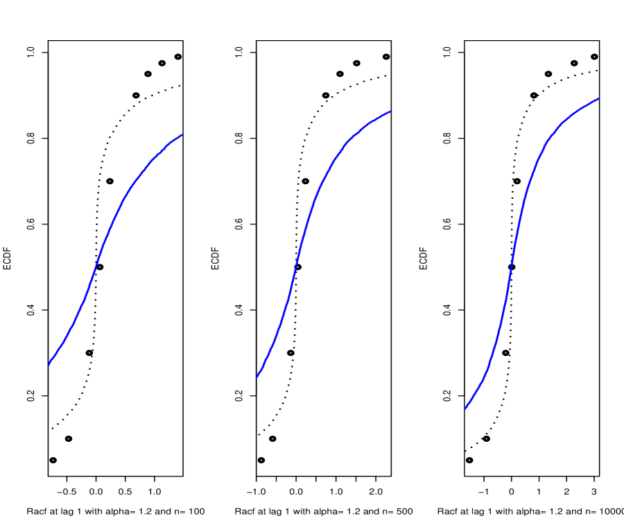
Figure 3: The slow convergence of residual autocorrelation to its asymptotic distribution. AR $(1)$ process, $X_{t}=0.5X_{t-1}+Z_{t}$, of series length $n=100$, $500$, $10^{4}$ were simulated respectively, where $\{Z_{t}\}$ is distributed as $Z_{1.2}(1,0,0)$. The number of simulation ${\rm~{}NSIM}=10^{4}$ were used. AR $(1)$ models were then fitted to simulated data and residual autocorrelation at lag one was calculated. The $5$, $10$, $30$, $50$, $70$, $90$, $95$, $97.5$, $99$ $(\%)$ empirical quantiles of residual autocorrelation at lag one were plotted as circles. The corresponding asymptotic distribution was plotted as the dot line. The asymptotic distribution of sample autocorrelation was plotted as the real line.

As in $\S$3.4, the slow convergence of $Q_{\rm BP}$ and $\hat{D}$ tests to their asymptotic distributions is also present at the residual autocorrelations. The first order autoregressive process $X_{t}=0.5X_{t-1}+Z_{t}$ with $Z_{t}\sim Z_{1.2}(1,0,0)$ was simulated and  AR $(1)$ models were fitted to the data. Then the 5, 10, 30, 50, 70, 90, 95, 97.5, 99 $(\%)$ empirical quantiles of $\hat{r}_{1}$ were plotted against its theoretical asymptotic distribution based on $10^{3}$ simulations. The asymptotic distribution of the error autocorrelation at lag one, $r_{1}$, was also plotted in Figure 3. It is seen that empirical quantiles of $\hat{r}_{1}$ get closer to its asymptotic distribution as the series length $n$ increases. However, this is not the case for the empirical quantiles of $\hat{r}_{1}$ to the asymptotic distribution of $r_{1}$. Therefore, serious size distortion may be present in this case if one uses error autocorrelations as a diagnostic tool for checking model adequacy. The slow convergence of residual autocorrelations to its asymptotic distribution may cause difficulties in using portmanteau tests in practice. Therefore, as in $\S$3.4, we suggested using the Monte-Carlo test to improve the effectiveness of portmanteau tests.

We now investigate the effectiveness of $Q_{\rm BP}$ and $\hat{D}$ tests for diagnostic check in fitted  AR  models with stable Paretian errors. The empirical sizes of $\hat{D}$ and $Q_{\rm BP}$ tests for a $5\%$ significance test were first calculated via simulation. In this experiment,  AR $(1)$ models, $X_{t}=\phi_{1}X_{t-1}+Z_{t}$, were simulated, where $Z_{t}\sim Z_{1.5}(1,0,0)$ and $\phi_{1}=0,\pm 0.1,\pm 0.3,\pm 0.5,\pm 0.7,\pm 0.9$ and  AR $(1)$ models were fitted to the simulated data by the Burg algorithm. The empirical size for each test was calculated based on $N=10^{4}$ simulations and each Monte Carlo test used $10^{3}$ simulations. Series length $n=100$ and lags $m=5,10,20$ were investigated. It is seen in Table 3 that the empirical sizes of both tests are very close to their nominal level.

[Table 3]

The empirical powers of $\hat{D}$ and $Q_{\rm BP}$ tests as diagnostic tools were also investigated via simulation. Twelve  ARMA $(2,2)$ models of series length $n=100$ in Table 4 of Peňa and Rodriguez (2002) were simulated and  AR $(1)$ models were fitted to the simulated data using the Burg algorithm. Both tests with lags $m=5,10,20$ were calculated using the parametric bootstrap procedure. The empirical powers were calculated based on $N=10^{3}$ simulations and each Monte Carlo test used $10^{3}$ simulations. It is seen in Table 4 that the empirical powers of both tests are reasonably good for most models. Some of them are even better than the powers listed in Peňa and Rodriguez (2002). In addition, increasing the series length can also improve the effectiveness of the proposed test procedure. For example, with model 3 in Table 2, if the series length was increased to $n=250$, the empirical powers of the $\hat{D}$ test at lags $m=5,10,20$ were increased significantly from 23.37%, 20.10% and 17.61% to 58.27%, 43.71% and 35.52%, respectively. Similar improvement was also found in the $Q_{\rm BP}$ test. Finally, as in Peňa and Rodriguez (2002), our simulation experiments show that $\hat{D}$ is more powerful than $Q_{\rm BP}$ as a diagnostic tool.

[Table 4]

Remark 5: It is well known that the Burg estimate of $\phi_{1}$ is close to the LS estimate. The advantage of using Burg estimate is that it is always in the stationary region and this is needed for the Monte-Carlo test.

4.3 Illustrative Application

Tsay (2002, Ch. 2) tentatively identified an AR(3) or AR(5) model for the monthly simple returns of CRSP value-weighted index from January 1926 to December 1997 using the partial autocorrelation function. Here $n=864$ and the usual Box-Pierce portmanteau test at lags $m=5,10,20$ does not suggest model inadequacy of either model at the 5% level. By applying our Monte-Carlo test procedure, however, both the $\hat{D}$ and $Q_{\rm BP}$ tests in §4 reject both models. The P-values are displayed in Table 5. The infinite variance hypothesis is plausible since the estimates for $\alpha$ of residuals in the fitted AR$(3)$ and AR$(5)$ models are 1.696 and 1.635, respectively. We may conclude from this example that using the ordinary portmanteau tests may lead to a wrong decision if innovations have infinite variance.

[Table 5]

5. CONCLUDING REMARK

We will provide an R package implementing the portmanteau tests described in this paper on CRAN.

APPENDIX A: PROOF OF THEOREM 1

First, by decomposing the determinant of the sample autocorrelation matrix $\textbf{R}_{(m)}$, Pena and Rodriguez (2002) showed that $|\textbf{R}_{(m)}|^{1/m}$ is a weighted function of the first $m$ partial autocorrelations. Specifically,

$$|\textbf{R}_{(m)}|^{1/m}=\prod^{m}_{i=1}(1-\pi^{2}_{i})^{(m+1-i)/m}.$$ (28)

Suppose that under the null hypothesis, $\hat{D}$ is asymptotic distributed as $\mathcal{X}$. By applying the $\delta$-method to $g(x)=\log(1-x)$, it follows that $-\left(n/\log(n)\right)^{2/\alpha}\,\log\left(|\textbf{R}_{(m)}|^{1/m}\right)$ is asymptotically distributed as $\mathcal{X}$. From eqn. (28), we can have

$$- \left(\frac{n}{\log(n)}\right)^{2/\alpha}\log\left(|\textbf{R}_{m}|^{1/m}\right)=$$ (29)

$$- \left(\frac{n}{\log(n)}\right)^{2/\alpha}\sum\limits_{i=1}^{m}\frac{m-i+1}{m}\log(1-{\pi}_{i}^{2}).$$

Next suppose that

$$\left(\frac{n}{\log(n)}\right)^{2/\alpha}\,\left({\pi}_{1}^{2},{\pi}_{2}^{2},\ldots,{\pi}_{m}^{2}\right)^{T}\longrightarrow Y,$$ (30)

and apply the multivariate $\delta$-method to

$$g({\pi}_{1}^{2},{\pi}_{2}^{2},\ldots,{\pi}_{m}^{2})=-\sum\limits_{i=1}^{m}\frac{m-i+1}{m}\log(1-{\pi}_{i}^{2}),$$

it follows that

$$-\sum\limits_{i=1}^{m}\frac{m-i+1}{m}\log(1-{\pi}_{i}^{2})\rightarrow\left(1,\frac{m-1}{m},\ldots,\frac{1}{m}\right)Y.$$ (31)

From the Cramer-Wold theorem, it follows that

$$\left(1,\frac{m-1}{m},\cdots,\frac{1}{m}\right)\left(\left(\frac{n}{\log(n)}\right)^{2/\alpha}\pi_{1}^{2},\ldots,\left(\frac{n}{\log(n)}\right)^{2/\alpha}\pi_{m}^{2}\right)^{T}$$

$$\longrightarrow\left(1,\frac{m-1}{m},\ldots,\frac{1}{m}\right)Y$$ (32)

By eqn. (14), it follows that

$$\left(1,\frac{m-1}{m},\ldots,\frac{1}{m}\right)\left(\left(\frac{n}{\log(n)}\right)^{2/\alpha}{\pi}_{1}^{2},\ldots,\left(\frac{n}{\log(n)}\right)^{2/\alpha}{\pi}_{m}^{2}\right)^{T}$$

$${\longrightarrow}W_{1}^{2}+\frac{m-1}{m}W^{2}_{2}+\ldots+\frac{1}{m}W_{m}^{2},$$ (33)

Finally, from eqn. (32) and eqn. (33),

$$\left(1,\frac{m-1}{m},\ldots,\frac{1}{m}\right)Y\rightarrow\sum^{m}_{i=1}\frac{m+1-i}{m}W^{2}_{i},$$

and from (30), we have the

$$\hat{D}\rightarrow\sum^{m}_{i=1}\frac{m+1-i}{m}W^{2}_{i}.\ \ \ \ \ \ \Box$$

APPENDIX B: MONTE-CARLO TEST PROCEDURE

The Monte-Carlo test procedure for diagnostic checking of AR and ARMA models with stable Paretian errors can be summarized below. Note that, to check randomness of a time series, we skip Step 1 and in Step 4 we simulate data from an IID sequence of $\{Z_{\hat{\alpha}}\}$ rather than from the fitted model.

Step 1

Fit an AR model to data using least-squares or the Burg algorithm or for ARMA, an approximate Gaussian maximum likelihood algorithm is used. Calculate residuals $\{\hat{Z}_{t}\}$ and the portmanteau test of interest , say $\hat{D}_{m}$.

Step 2

Estimate $\alpha$ from residuals $\{\hat{Z}_{t}\}$ in Step 1. The estimator given by McCulloch (1986) may be used.

Step 3

Select the number of Monte-Carlo simulations, $B$. Typically $100\leq B\leq 1000$.

Step 4

Simulate the fitted model using the estimated AR or ARMA parameters in Step 1 and $\hat{\alpha}$ in Step 2. Obtain $\hat{D}_{m}$ after estimating the parameters in the simulated series.

Step 5

Repeat Step 4 $B$ times counting the number of times $k$ that a value of $\hat{D}_{m}$ greater than or equal to that in Step 1 has been obtained.

Step 6

The $P$-value for the test is $(k+1)/(B+1)$.

Step 7

Reject the null hypothesis if the $P$-value is smaller than a predetermined significance level.

APPENDIX C: THE GENERALIZATION OF LINEAR EXPANSION OF RESIDUAL AUTOCORRELATION

C.1 Introduction

Residual autocorrelations are an important tool for diagnostic checking of autoregressive and moving average ( ARMA ) models. Their asymptotic distributions from univariate  ARMA  models were first derived by Box and Pierce (1970). McLeod (1978) refined the derivation and extended it to the multiplicative seasonal ARMA  models. Their results were established under the assumption that error sequences have finite variance and the parameters are estimated using least squares, or equivalently, using maximum likelihood estimation (MLE) for Gaussian  ARMA  processes. Their result may not be valid if the parameters of interest are estimated using other estimation methods or linear processes with infinite variance. This section demonstrates how the linear expansion of residual autocorrelations in Box and Pierce (1970) also holds for other estimation methods and for  AR  models with stable Paretian errors. The expansion may be used to derive the limiting distribution of residual autocorrelations.

C.2 The Autoregressive Process

Consider an  AR $(p)$ process as follows:

$$\phi(B)y_{t}=a_{t},$$ (34)

where $B$ denotes the backward operator, $\phi(B)=1-\phi_{1}B-\cdots-\phi_{p}B^{p}$, and $\{a_{t}\}$ is a sequence of independent and identical random variables with mean zero and finite variance $\sigma_{a}^{2}$. For given values $\dot{\Phi}=\left(\dot{\phi}_{1},\cdots,\dot{\phi}_{p}\right)^{T}$ of parameters, we can define

$$\dot{a}_{t}=a_{t}(\dot{\Phi})=y_{t}-\dot{\phi}_{1}y_{t-1}-\cdots-\dot{\phi}_{p}y_{t-p}=\dot{\Phi}(B)y_{t}$$ (35)

and the corresponding autocorrelation function at lag $k$ as

$$\dot{r}_{k}=r_{k}(\dot{\Phi})=\frac{\sum\dot{a}_{t}\dot{a}_{t-k}}{\sum\dot{a}^{2}_{t}}.$$ (36)

C.3 Linear Expansion of Residual Autocorrelation Function about Error Autocorrelation Functions

Consider approximating the residual autocorrelation $\hat{r}_{k}$ by a first order Taylor expansion about $\hat{\Phi}=\Phi$. Let $\dot{c}_{k}$ and $\dot{r_{k}}$ denote $\sum\dot{a}_{t}\dot{a}_{t-k}$ and $\dot{c}_{k}/\dot{c}_{0}$ respectively, where $k\in$ integer. Consider the estimators of $\Phi$ satisfying

$$\hat{\phi}_{j}=\phi_{j}+O_{p}\left(1/\sqrt{n}\right),\ \forall\ j.$$ (37)

We have

$$\hat{r}_{k}=r_{k}+\sum^{p}_{j=1}\left(\phi_{j}-\hat{\phi}_{j}\right)\hat{\delta}_{jk}+O_{p}\left(1/n\right),$$ (38)

where

$$\hat{\delta}_{jk} = -\frac{\partial\dot{r}_{k}}{\partial\dot{\phi}_{j}}|_{\dot{\Phi}=\hat{\Phi}}$$ (39)

$$= -\frac{\partial}{\partial\dot{\phi}_{j}}\left(\frac{\dot{c}_{k}}{\dot{c}_{0}}\right)|_{\dot{\Phi}=\hat{\Phi}}$$

$$= \hat{\delta}^{(1)}_{ij}+\hat{\delta}^{(2)}_{ij},$$

$$\hat{\delta}^{(1)}_{ij}=-\dot{c}_{k}\frac{\partial}{\partial\dot{\phi}_{j}}\left(\frac{1}{\dot{c}_{0}}\right)|_{\dot{\Phi}=\hat{\Phi}}$$

and

$$\hat{\delta}^{(2)}_{ij}=-\frac{1}{\dot{c}_{0}}\frac{\partial\dot{c}_{k}}{\partial\dot{\phi}_{j}}|_{\dot{\Phi}=\hat{\Phi}}.$$

For LS estimates, we have that

$$\frac{\partial}{\partial\dot{\phi}_{j}}\left[\sum\dot{a}_{t}^{2}\right]|_{\dot{\Phi}=\hat{\Phi}}=\frac{\partial c_{0}}{\partial\dot{\phi}_{j}}|_{\dot{\Phi}=\hat{\Phi}}=0$$ (40)

so it is straightforward that $\hat{\delta}_{ij}^{(1)}=0$. Using this result, Box and Pierce (1970) showed that $\hat{\delta}_{jk}=\psi_{k-j}$ to order $O_{p}\left(n^{-1/2}\right)$, where $\psi_{j}$’s are the impulse response coefficients of the  MA $(\infty)$ representation of eqn. (34). For other estimation methods, however, $\hat{\delta}^{(1)}_{ij}$ may not be zero since eqn. (40) does not hold. To obtain a general result for $\hat{\delta}_{ij}$, therefore, we will calculate $\hat{\delta}^{(1)}_{ij}$ explicitly.

Note that $\hat{\delta}^{(1)}_{ij}$ can be written as follows:

$$\dot{c}_{k}\cdot\left[\sum\dot{a}_{t}^{2}\right]^{-2}\frac{\partial\dot{c}_{0}}{\partial\dot{\phi}_{j}}|_{\dot{\Phi}=\hat{\Phi}}.$$ (41)

By eqn. (2.15) of Box and Pierce (1970) and letting $k=0$, eqn. (41) can be expressed as follows:

$$\frac{\sum y_{t}^{2}}{\sum\hat{a_{t}^{2}}}\cdot\sum_{i=0}^{p}\hat{\phi}_{i}\left[r^{(y)}_{-i+j}+r^{(y)}_{i-j}\right]\cdot\frac{\hat{c}_{k}}{\hat{c}_{0}}$$ (42)

$$= \frac{\sum_{i=0}^{p}\hat{\phi}_{i}\left[r^{(y)}_{-i+j}+r^{(y)}_{i-j}\right]}{\sum_{i=0}^{p}\sum_{j=0}^{p}\hat{\phi}_{i}\hat{\phi}_{j}r^{(y)}_{i-j}}\cdot\hat{r}_{k},$$

where

$$r_{\nu}^{(y)}=\frac{\sum y_{t}y_{t-\nu}}{\sum y_{t}^{2}}.$$

Let $\hat{\zeta}_{j}$ denote

$$\left({\sum_{i=0}^{p}\hat{\phi}_{i}\left[r^{(y)}_{-i+j}+r^{(y)}_{i-j}\right]}\right)/\left({\sum_{i=0}^{p}\sum_{j=0}^{p}\hat{\phi}_{i}\hat{\phi}_{j}r^{(y)}_{i-j}}\right),$$

and approximate $\hat{\zeta}_{j}$ by replacing $\hat{\phi}$’s and $r^{(y)}$’s with $\phi$’s and $\rho$’s, the theoretical parameters and the autocorrelations of the autoregressive process $\{y_{t}\}$. By the Barteltt’s formula,

$$r_{k}^{(y)}=\rho_{k}+O_{p}\left(1/\sqrt{n}\right)$$

as well as eqn. (37) and (42), we have

$$\hat{\zeta}_{j}=\zeta_{j}+O_{p}\left(1/\sqrt{n}\right).$$ (43)

Then by making use of the recursive relation which is satisfied by the autocorrelations of an autoregressive process, eqn. (2.19) of Box and Pierce (1970), or

$$\rho_{\nu}-\phi_{1}\rho_{\nu-1}-\cdots-\phi_{p}\rho_{\nu-p}=\phi(B)\rho_{\nu}=0,\ \ \ \ \nu\geq 1,$$ (44)

$\zeta_{j}$ can be simplified to yield

$$\zeta_{j}=\frac{\sum_{i=0}^{p}\phi_{i}\rho_{-j+i}}{\sum_{i=0}^{p}\phi_{i}\rho_{i}}.$$ (45)

Note that eqn. (45) has the same form of eqn. (2.20) of Box and Pierce (1970). Specifically, it can be seen as $\delta_{-j}$. Moreover, Box and Pierce indicated that $\delta_{\nu}=0,\ \nu<0$ so $\zeta_{j}=0$. Plugging this result into eqn. (42), we have $\hat{\delta}^{(1)}_{ij}=0$. Consequently, eqn. (2.20) of Box and Pierce (1970) for the linear expansion of residual autocorrelations still holds for other estimators with order $\hat{\phi}_{i}-\phi=O_{p}(1/\sqrt{n})$.

Remark 6 : Many estimators of $\phi_{(p)}$ for an  AR  model with Paretian stable errors have order $O_{p}([n/\log(n)]^{-1/\alpha})$, such as Whittle’s, Yule-Walker and LS estimtors. Using the result that $\textbf{r}_{(p)}=\rho_{(p)}+O_{p}([n/\log(n)]^{-1/\alpha})$, and following the proofs in this section as well as in Box and Pierce (1970), we may obtain the linear expansion of residual autocorrelation functions for  AR  models with stable Paretian errors as in eqn. (19)

C.4 The Equality of Residuals in  AR  and  ARIMA  Models

The result in $\S C$.3 may be extended to  ARIMA  models using technique in $\S$5.1 of Box and Pierce (1970). If two time series (a) an  ARMA ($p,q$) process

$$\phi(B)w_{t}=\theta(B)a_{t},$$ (46)

and (b) an autoregressive series

$$\pi(B)x_{t}=\left(1-\pi_{1}B-\cdots-\pi_{p+q}B^{p+q}\right)x_{t}=a_{t},$$ (47)

are both generated from the same set of errors $\{a_{t}\}$, where

$$\phi(B)=1-\phi B-\phi B^{2}-\cdots-\phi B^{p},$$

and

$$\theta(B)=1-\theta B-\theta B^{2}-\cdots-\theta B^{q}.$$

If

$$\pi(B)=\phi(B)\theta(B),$$ (48)

then when the models are fitted by least squares, their residuals, and hence also their autocorrelations, will be very nearly the same. In this section, we consider whether the equality of residuals between  AR  and  ARIMA  models is still valid when the parameters are estimated by other approaches.

As in eqn. (35), define

$$\dot{a}^{AR}_{t}=a_{t}^{AR}(\dot{\pi})=\dot{\pi}(B)x_{t}=-\sum_{j=0}^{p+q}\dot{\pi}_{j}x_{t-j},$$ (49)

where $\dot{\pi}_{0}=-1$, and now also

$$\dot{a}^{\star}_{t}=a_{t}^{\star}(\dot{\phi},\dot{\theta})=\dot{\phi}(B)\dot{\theta}(B)^{-1}w_{t}=\left[\sum^{p}_{i=0}\dot{\phi}_{i}B^{i}\right]\left[\sum_{j=0}^{q}\dot{\theta}_{j}B^{j}\right]^{-1}w_{t},$$ (50)

where $\dot{\phi}_{0}=\dot{\theta}_{0}=-1$. Using eqn. (5.12) and eqn. (5.13) of Box and Pierce (1970), we can approximate $a^{AR}_{t}$ and $a^{\star}_{t}$ as follows:

$$\dot{\mathbf{a}}^{AR}=\mathbf{a}+\mathbf{X}\left(\pi-\dot{\pi}\right)$$ (51)

and

$$\dot{\mathbf{a}}^{\star}=\mathbf{a}+\mathbf{X}\left(\beta-\dot{\beta}\right).$$ (52)

Note that eqn. (51) and eqn. (52) can be seen as a linear regression model. We can estimate regression coefficients, $\pi-\dot{\pi}$ and $\beta-\dot{\beta}$ using any suitable method. Let $g(\mathbf{X},\dot{\mathbf{a}}^{\bullet})$ denote the corresponding estimator. Since both eqn. (51) and eqn. (52) have the same form, their estimators should agree with each other. For example, least squares estimates are given by

$$\hat{\pi}-\dot{\pi}=g(\mathbf{X},\dot{\mathbf{a}}^{AR})=(\mathbf{X}^{T}\mathbf{X})^{-1}\mathbf{X}^{T}\dot{\mathbf{a}}^{AR}$$ (53)

and

$$\hat{\beta}-\dot{\beta}=g(\mathbf{X},\dot{\mathbf{a}}^{\star})=(\mathbf{X}^{T}\mathbf{X})^{-1}\mathbf{X}^{T}\dot{\mathbf{a}}^{\star}.$$ (54)

Then by setting $\dot{\mathbf{a}}=\mathbf{a}$ and estimating the regression coefficients of eqn. (51) and eqn. (52), we have

$$\hat{\pi}-\pi=g(\mathbf{X},\mathbf{a})=\hat{\beta}-\beta.$$ (55)

Finally, by setting $\dot{\mathbf{a}}^{AR}=\hat{\mathbf{a}}^{AR}$ and $\dot{\mathbf{a}}^{\star}=\hat{\mathbf{a}}^{\star}$ in eqn. (51) and eqn. (52), it follows from eqn. (55) that to order $O_{p}\left(|\hat{\beta}-\beta|^{2}\right)$

$$\hat{\mathbf{a}}^{AR}=g(\mathbf{X},\mathbf{a})=\hat{\mathbf{a}}^{\star},$$ (56)

and thus (to the same order) $\hat{r}^{AR}=\hat{r}^{\star}$.

REFERENCES

Adler, R.J. Feldman, R.E. and Gallagher, C. (1998), “Analysing Stable Time Series,” A Practical Guide to Heavy Tails: Statistical Techniques and Applications, Birkh$\ddot{a}$user, Boston.

Box, G.E.P. and Pierce, D.A. (1970), “Distribution of Residual Autocorrelation in Autoregressive-Integrated Moving Average Time Series Models,” Journal of American Statistical Association 65, 1509-1526.

Brockwell, P.J. and Davis, R.A. (1991), Time Series: Theory and Methods, Springer, New York.

Davis, R.A. (1996), “Gauss-Newton and M-estimation for  ARMA  processes,” Stochastic Processes and their Applications 63, 75–95.

Davis, R.A. and Resnick, S. (1986), “Limit Theory for the Sample Covariance and Correlation Functions of Moving Averages,” The Annals of Statistics 14, 533–558.

McCulloch, J.H. (1986), “Simple Consistent Estimators of Stable Distribution Parameters,” Communication in Statistics–Computation and Simulation, 15, 1109–1136.

Mittnik, S., Rachev, S.T., Doganoglu, T. and Chenyao, D. (1999), “Maximum Likelihood Estimation of Stable Paretian Models,” Mathematical and Computer Modelling, 29, 275–293.

Monti, A.C. (1994), “A Proposal for Residual Autocorrelation Test in Linear Models,” Biometrika 81, 776–780.

Peňa, D. and Rodriguez, J. (2002), “A Powerful Portmanteau Test of Lack of Fit For Time Series,” Journal of American Statistical Association 97, 601-610.

Runde, R. (1997), “The Asymptotic Null Distribution of the Box-Pierce Q-Statistic for Random Variable with Infinite Variance: An Application to German Stock Returns,” Journal of Econometrics 78, 205-216.

Samorodnitsky, G. and Taqqu, M. (1994), Stable-Non-Gaussian Random Processes, Chapman-Hall, New York.

Tsay, R.S. (2002), Analysis of Financial Time Series, New York: Wiley.

Table I. Empirical sizes $(\%)$ of $\hat{D}$ and $Q_{\rm BP}$ for a $5\%$ significance test based on the parametric bootstrap procedure. The empirical size for each test was calculated based on $N=10^{4}$ simulations. Each Monte Carlo test also used $B=10^{3}$ simulations. Series length $n=250$ and lags $m=5,10,15$ were investigated.

	$\hat{D}(5)$	$\hat{D}(10)$	$\hat{D}(15)$	$Q_{\rm BP}(5)$	$Q_{\rm BP}(10)$	$Q_{\rm BP}(15)$
$\alpha=1.9$	$5.30$	$4.66$	$4.78$	$4.96$	$4.71$	$4.87$
$\alpha=1.7$	$5.18$	$4.44$	$4.44$	$4.82$	$4.43$	$4.41$
$\alpha=1.5$	$4.82$	$4.99$	$5.13$	$5.07$	$5.27$	$5.30$
$\alpha=1.3$	$4.80$	$5.03$	$5.18$	$5.04$	$5.00$	$5.27$
$\alpha=1.1$	$5.26$	$5.33$	$5.12$	$5.33$	$5.25$	$5.15$

Table II. P-values for $Q_{\rm LB}$ statistic using Monte-Carlo test and $\chi^{2}$-method for testing randomness of exchange-rate returns.

	Monte-Carlo Test	$\chi^{2}(m)$ Test
$m=5$	$0.500$	$0.042$
$m=10$	$0.582$	$0.228$
$m=20$	$0.828$	$0.404$

Table III. Empirical sizes $(\%)$ of $\hat{D}$ and $Q_{\rm BP}$ for a $5\%$ significance test. $\hat{D}$ and $Q_{\rm BP}$ tests for checking model adequacy of  AR $(1)$ models fitted by the Burg algorithm. Both tests were implemented by the parametric bootstrap procedure. The empirical size for each test was calculated based on $N=10^{4}$ simulations. Each Monte Carlo test also used $B=10^{3}$ simulations. Series length $n=100$ and lags $m=5,10,20$ were investigated.

$\phi_{1}$	$\hat{D}(5)$	$\hat{D}(10)$	$\hat{D}(20)$	$Q_{\rm BP}(5)$	$Q_{\rm BP}(10)$	$Q_{\rm BP}(20)$
$0.9$	$4.90$	$4.75$	$4.88$	$4.60$	$4.71$	$4.96$
$0.7$	$4.97$	$5.20$	$5.16$	$4.95$	$4.94$	$5.42$
$0.5$	$5.37$	$5.32$	$5.14$	$5.55$	$5.12$	$5.16$
$0.3$	$5.11$	$4.90$	$4.82$	$5.13$	$4.80$	$5.26$
$0.1$	$4.92$	$5.01$	$5.20$	$5.14$	$4.75$	$4.86$
$-0.1$	$5.30$	$5.45$	$5.29$	$5.25$	$5.08$	$4.90$
$-0.3$	$5.00$	$5.20$	$5.33$	$4.79$	$5.30$	$5.45$
$-0.5$	$5.00$	$4.93$	$5.10$	$5.00$	$4.93$	$5.26$
$-0.7$	$5.62$	$5.73$	$5.65$	$5.20$	$5.45$	$5.41$
$-0.9$	$5.21$	$5.02$	$5.07$	$5.01$	$5.00$	$5.30$

Table IV. Empirical powers $(\%)$ of $\hat{D}$ and $Q_{\rm BP}$ for a $5\%$ significance test. $\hat{D}$ and $Q_{\rm BP}$ tests for checking model adequacy of twelve  ARMA $(2,2)$ models in Table 3 of Peňa and Rodriguez (2002) fitted by  AR $(1)$ using the Burg algorithm. Both tests were implemented based on the parametric bootstrap procedure. The empirical power for each test was calculated based on $N=10^{4}$ simulations. Each Monte Carlo test also used $B=10^{3}$ simulations. Series length $n=100$ and lags $m=5,10,20$ were investigated.

Model	$\hat{D}(5)$	$\hat{D}(10)$	$\hat{D}(20)$	$Q_{\rm BP}(5)$	$Q_{\rm BP}(10)$	$Q_{\rm BP}(20)$
1	$53.32$	$38.31$	$32.77$	$29.59$	$21.76$	$19.25$
2	$99.01$	$98.56$	$98.01$	$94.53$	$70.46$	$59.61$
3	$23.37$	$20.10$	$17.61$	$21.62$	$16.71$	$15.17$
4	$77.13$	$59.38$	$48.12$	$60.82$	$40.29$	$35.15$
5	$93.22$	$87.62$	$79.84$	$84.66$	$66.68$	$58.46$
6	$13.74$	$11.17$	$10.05$	$10.68$	$9.13$	$8.61$
7	$26.51$	$26.25$	$24.92$	$17.56$	$13.80$	$13.05$
8	$33.92$	$26.68$	$23.57$	$27.36$	$20.60$	$19.25$
9	$99.44$	$99.27$	$99.16$	$98.71$	$93.17$	$78.88$
10	$76.71$	$58.06$	$48.50$	$40.62$	$28.39$	$25.94$
11	$99.01$	$98.46$	$97.87$	$94.02$	$67.04$	$57.11$
12	$99.89$	$99.87$	$99.48$	$99.86$	$99.63$	$99.48$

Table V. An illustrated example using the monthly simple return of CRSP value-weighted index data from Tsay (2002). The data were fitted by an AR$(3)$ model and an AR$(5)$ model. The entries in the first two columns are the P-values of $\hat{D}$ and $Q_{\rm BP}$ in §4 based on the Monte-Carlo test; those in the third column are the P-value of the portmanteau test of Box and Pierce (1970) assuming a normal distribution, denoted by $Q^{\rm N}_{\rm BP}$.

	AR $(3)$
	$\hat{D}$	$Q_{\rm BP}$	$Q_{\rm BP}^{\rm N}$
$m=5$	$0.050$	$0.026$	$0.197$
$m=10$	$0.030$	$0.021$	$0.107$
$m=20$	$0.019$	$0.012$	$0.247$
	AR $(5)$
	$\hat{D}$	$Q_{\rm BP}$	$Q_{\rm BP}^{\rm N}$
$m=5$	$0.064$	$0.055$	$0.998$
$m=10$	$0.052$	$0.045$	$0.345$
$m=20$	$0.024$	$0.024$	$0.438$

Figure 1: The slow convergence of the $\hat{D}$ test to its asymptotic distribution. Random sequences of series length $n=10^{3},2000,5000,10^{4}$ were simulated from $S_{1.5}(1,0,0)$. $250$ simulations were used to retrieve empirical percentiles of the $\hat{D}$ test with $m=5$. The $5$, $10$, $30$, $50$, $70$, $90$, $95$, $97.5$, $99$ $(\%)$ empirical quantiles were plotted as black circles and the corresponding asymptotic distribution was also plotted as the dot line.

Figure 2: The slow convergence of the $Q_{\rm BP}$ test to its asymptotic distribution. Random sequences of series length $n=10^{3},2000,5000,10^{4}$ were simulated from $S_{1.5}(1,0,0)$. $250$ simulations were used to retrieve empirical percentiles of the $Q_{\rm BP}$ test with $m=5$. The $5$, $10$, $30$, $50$, $70$, $90$, $95$, $97.5$, $99$ $(\%)$ empirical quantiles were plotted as circles and the corresponding asymptotic distribution was also plotted as the dot line.