Improved Peňa-Rodriguez Portmanteau Test

 

Abstract

Several problems with the diagnostic check suggested by Peňa and Rodriguez (2002) are noted and an improved Monte-Carlo version of this test is suggested. It is shown that quite often the test statistic recommended by Peňa and Rodriguez (2002) may not exist and their asymptotic distribution of the test does not agree with the suggested gamma approximation very well if the number of lags used by the test is small. It is shown that the convergence of this test statistic to its asymptotic distribution may be quite slow when the series length is less than 1000 and so a Monte-Carlo test is recommended. Simulation experiments suggest the Monte-Carlo test is usually more powerful than the test given by Peňa and Rodriguez (2002) and often much more powerful that the Box-Ljung portmanteau test. Two illustrative examples of enhanced diagnostic checking with the Monte-Carlo test are given.

Keywords: ARMA residual diagnostic test; Imhof distribution; Monte-Carlo test; Portmanteau diagnostic check

 

1. Introduction

Let $X_{t},t=1,2,\ldots$ be a stationary and invertible  ARMA ($p,q$) model (Box, Jenkins, and Reinsel, 1994),

$$(1-\phi_{1}B-\cdots-\phi_{p}B^{p})X_{t}=(1-\theta_{1}B-\cdots-\theta_{q}B^{q})a_{t},$$ (1)

where $B$ is the backshift operator on $t$, $a_{t}$ is a sequence of independent and identical normal random variables with mean zero and variance $\sigma_{a}^{2}$. After fitting this model to a series of length $n$, the residual autocorrelations,

$$\hat{r}(k)=\sum_{t=k+1}^{n}\hat{a}_{t}\hat{a}_{t-k}/\sum_{t=1}^{n}\hat{a}_{t}^{2}\ \ \ \ k=1,2,\cdots,$$ (2)

where $\hat{a}_{t}$ denotes the fitted residuals, may be used for checking model adequacy. One of the most widely used model diagnostic checks (Li, 2004) is the portmanteau test of Ljung and Box (1978),

$$Q_{m}=n(n+2)\sum_{k=1}^{m}(n-k)^{-1}\hat{r}(k)^{2},$$ (3)

where, under the assumption of model adequacy, $Q_{m}$ is approximately $\chi^{2}_{m-(p+q)}$ distributed.

A new portmanteau diagnostic test statistic, $\hat{D}_{m}=n(1-|\hat{R}_{m}|^{1/m})$, based on the determinant of the residual autocorrelation matrix,

$$\hat{R}_{m}=\left(\begin{array}[]{cccc}1&\hat{r}(1)&\cdots&\hat{r}(m)\\ \hat{r}(1)&1&\cdots&\hat{r}(m-1)\\ \vdots&\cdots&\ddots&\vdots\\ \hat{r}(m)&\cdots&\hat{r}(1)&1\end{array}\right),$$ (4)

was suggested by Peňa and Rodriguez (2002). As noted by Peňa and Rodriguez (2002), $|\hat{R}_{m}|$ is the estimated generalized variance of the residuals standardized by dividing by their standard deviation.

2. THE $D_{m}$ TEST AND ITS LIMITATIONS

Peňa and Rodriguez (2002, Theorem 1) showed that if the model is correctly identified, $\hat{D}_{m}$ is asymptotically distributed as $\sum\limits_{i=1}^{m}\lambda_{i}\chi_{1,i}^{2}$, where $\chi_{1,i}^{2}$ are independent Chi-squared random variables with one degree of freedom, and $\lambda_{i}$ are the eigenvalues of ${\cal Q}_{m}W_{m}$, where $W_{m}$ is a diagonal matrix with the $i$-th diagonal elements, $w_{i}=(m-i+1)/m$, $i=1,2,\ldots,m$ and ${\cal Q}_{m}$ is the asymptotic covariance matrix of the normalized residual autocorrelations $\surd{n}(\hat{r}(1),\ldots,\hat{r}(m))$ given in McLeod (1978, eqn. 15). As pointed out by Peňa and Rodriguez (2002), this asymptotic distribution may be computed using the method of Imhof (1961). We have implemented the computation of this asymptotic distribution for the general ARMA$(p,q)$ model in our R package gvtest. The cumulative distribution function for this asymptotic distribution may be denoted by $F(x;\lambda_{1},\ldots,\lambda_{m})$.

Peňa and Rodriguez (2002) suggested evaluating $\hat{D}_{m}$ by a gamma approximation distribution to the asymptotic distribution. The approximation distribution is derived by equating the first two moments of a gamma distribution with those of the corresponding asymptotic distribution. The density function for this gamma approximation may be written $f_{\gamma}(x;\alpha,\beta)=e^{-\frac{x}{\beta}}x^{\alpha-1}\beta^{-\alpha}/\Gamma(\alpha)$ where,

$$\alpha=3\left.m\{\left(m+1\right)-2\left(p+q\right)\right\}^{2}/\left[2\{2\left(m+1\right)\left(2m+1\right)-12m(p+q)\}\right],$$ (5)

and

$$\beta=3\left.m\{\left(m+1\right)-2\left(p+q\right)\right\}/\left\{2\left(m+1\right)\left(2m+1\right)-12m(p+q)\right\}.$$ (6)

Peňa and Rodriguez (2002) indicated that the approximation improves as $m$ increases. In addition, it may be noted that if $m$ is too small then it can happen that $\alpha\leq 0$ or $\beta\leq 0$ which is numerically infeasible. For example if $p+q=3$ then we must have $m\geq 8$ to make $\alpha>0$ and $\beta>0$.

Peňa and Rodriguez (2002) found that the empirical distribution of $\hat{D}_{m}$ did not agree very well with the gamma approximation so they suggested a modified statistic,

$$D_{m}=n-n|\ddot{R}_{m}|^{\frac{1}{m}},$$ (7)

where $\ddot{R}_{m}$ denotes the residual autocorrelation matrix replacing $\hat{r}(k)^{2}$ with $\ddot{r}_{k}^{2}$, where

$$\ddot{r}(k)^{2}=\left(n+2\right)\left(n-k\right)^{-1}\hat{r}(k)^{2}.$$

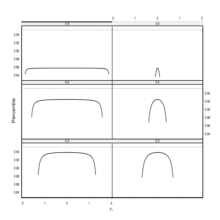
Figure 1: Inaccuracy of the gamma approximation for AR(2) with $m=10$. $F(Q_{\gamma}(0.05;\alpha,\beta);\lambda_{1},\ldots,\lambda_{1}0)$, where $F$ is the cdf of asymptotic distribution of $\hat{D}_{m}$ and $Q_{\gamma}$ is the quantile function for the gamma approximation, is plotted. The plot shows panels corresponding to $\phi_{2}=\pm 0.3,\pm 0.6,\pm 0.9$. The parameter $\phi_{1}$ extends over the whole admissible region corresponding to the $\phi_{2}$. These plots demonstrate that the gamma approximation is not conservative asymptotically. When $n$ is large enough, the test based on the gamma approximation will overstate the true significance level.

This is similar in spirit to the modification suggested by Ljung and Box (1978) to the original Box and Pierce portmanteau statistic (1970). Although, as shown by Peňa and Rodriguez (2002), this approximation works well when $n\leq 100$ in first order autoregressive models, it does not provide a good approximation to the asymptotic distribution for more complicated models if the number of lags, $m$, is small. As shown in Figure 1, the gamma approximation can distort the size of a 5% significance test relative to the asymptotic distribution for  AR $(2)$ models when $m$ is $10$. Similar distortions are found for  MA $(2)$ models or higher orders  AR  and  MA  models. The distortions for  ARMA $(1,1)$ with $m=10$ models were also investigated and the results were listed in Table 1. Moreover, this distortion would tend to make the tests based on the gamma approximation reject more often than they should. In other words, the test based on the gamma approximation is not conservative. So despite the fact that as shown by Peňa and Rodriguez (2002, Table 2) the small sample performance is acceptable in some cases, the more general use of tests based on the gamma approximation can not be recommended. The reader may investigate the accuracy of the gamma approximation for a particular $m$ and ARMA$(p,q)$ using our gvtest package.

[Table 1 about here]

Another serious limitation to the use of $D_{m}$ is that it is frequently undefined. This happens because $\ddot{R}_{m}$ is not always positive-definite (McLeod and Jiménez, 1984). When we tried to replicate Table 4 in Peňa and Rodriguez (2002) we frequently found cases where $\ddot{R}_{m}$ was not positive-definite. For example, for model 7 listed in this table this happens about 25% of the time with $m=10$. This problem occurred with many other models listed in this table. Although only very short time series were used in Table 4, this problem also occurs with longer time series particularly when $m$ is also larger. For this reason, it is better to concentrate on the original $\hat{D}_{m}$ statistic.

[Figure 1 about here]

3. TESTS BASED ON $\hat{D}_{m}$

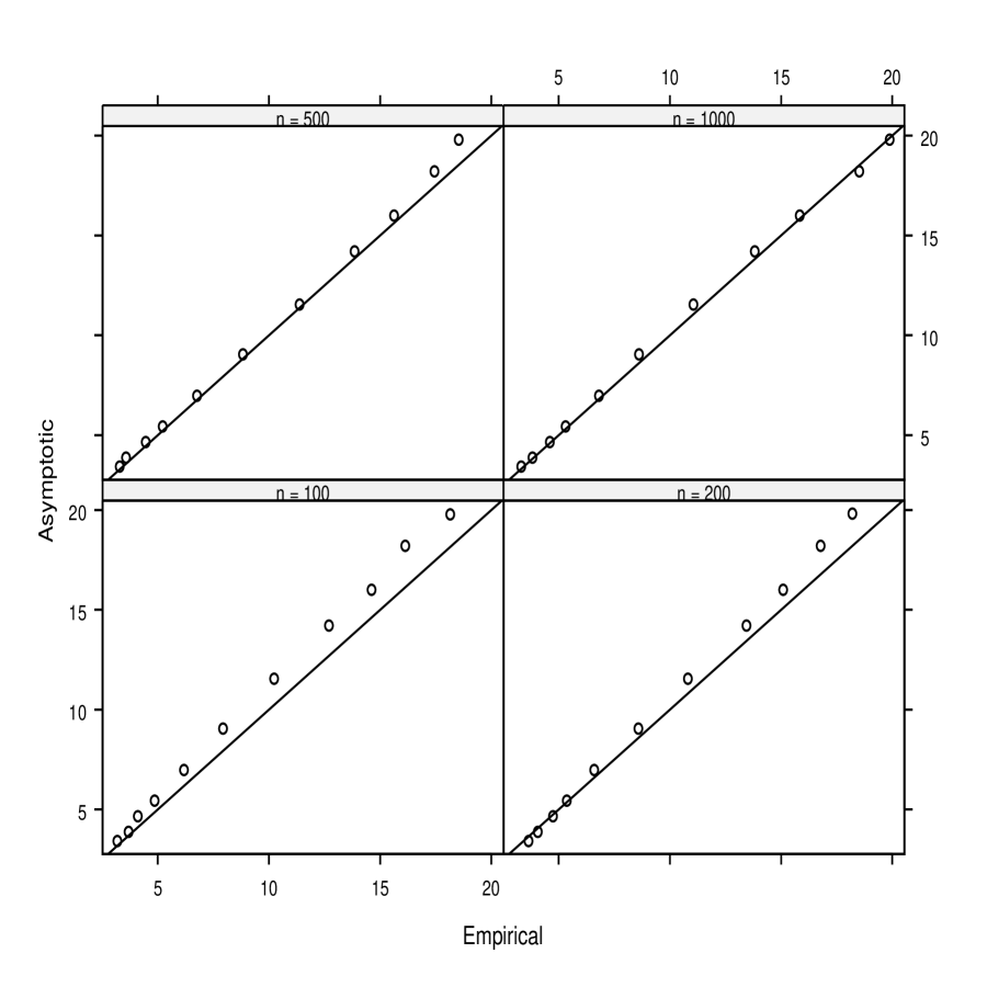
Figure 2: Slow convergence of empirical distribution of $\hat{D}_{m}$. The AR$(1)$ with parameter $\phi_{1}=0.5$ was simulated $10^{3}$ times for series of lengths $n=100,200,500,1000$ and the empirical distribution of $\hat{D}_{m}$ with $m=20$ was compared with its asymptotic distribution using a QQ plot with quantiles corresponding to 0.01, 0.02, 0.05, 0.1, 0.2, 0.5, 0.7, 0.9, 0.95, 0.98, 0.99.

In a modern high level computing environment, such as R or Mathematica, it is not difficult to evaluate the asymptotic distribution and so a test based directly on this asymptotic distribution might seem to be preferable. Unfortunately, the convergence of $\hat{D}_{m}$ to its asymptotic distribution is often very slow. In Table 2, we evaluated the asymptotic distribution corresponding to the upper 5% point of the empirical distribution of $\hat{D}_{m}$ for the first-order autoregressions with series lengths $n=100,200,500$ and 1000. Not until $n$ is very large is the asymptotic distribution reliable. Figure 2 shows a QQ plot for these simulations which shows that the discrepancy between the empirical and asymptotic distribution increases at the larger quantiles. The asymptotic distribution tends to understate the actual finite-sample significance level while the gamma approximation errs in the opposite direction.

For these reasons, a Monte-Carlo test procedure (Gentle, 2002, §2.3) is recommended when $n<1000$. This procedure is quite practical on typical computers now available. This test is essentially equivalent to a parametric bootstrap test (Davison and Hinkley, 1997, Ch.4). The steps in the procedure are indicated below:

1. After fitting model in eqn. (1) obtain $\hat{D}_{m}$.

2. Select the number of Monte-Carlo simulations, $N$. Typically $100\leq N\leq 1000$.

3. Simulate the model in eqn. (1) using the estimated parameters obtained in Step 1 and obtain $\hat{D}_{m}$ after estimating the parameters in the simulated series.

4. Repeat Step 3 $N$ times counting the number of times $k$ that a value of $\hat{D}_{m}$ greater than or equal to that in Step 1 has been obtained.

5. The $P$-value for the test is $(k+1)/(N+1)$.

6. Reject the null hypothesis if the $P$-value is smaller than a predetermined significance level.

It should be noted that nuisance parameters are present in our proposed procedure and this could cause size distortion in the Monte Carlo test (Jöckel, 1986). The empirical size of the Monte-Carlo test for the first order autoregressive model was investigated by simulation. The results were summarized in Table 3 and it is seen that the empirical sizes are very close to their nominal level. In general, it has been shown (Dufour, 2006; Dufour and Khalaf, 2001) that if consistent estimators are used then the Monte-Carlo test produces an asymptotically correct size as $n\rightarrow\infty$. The asymptotic validity of the Monte-Carlo test follows immediately. Alternatively since the gamma approximation is asymptotically correct as both $n$ and $m$ get large, it follows that $\hat{D}_{m}$ is asymptotically pivotal and hence does not depend on nuisance parameters.

[Figure 2 and Table 2,3 about here]

4. EMPIRICAL POWER COMPARISONS

In many cases the Monte-Carlo test outperforms the the $D_{m}$ test based on the gamma approximation. As an illustration, in Table 4 the simulation results for the Monte-Carlo test are compared with $D_{m}$ test for the GARCH models Peňa and Rodriguez (2002, Table 12). We see that the Monte-Carlo test has always has higher power than the gamma approximation in Table 4.

Peňa and Rodriguez (2002) indicated that the advantage of their test over the Ljung-Box test, denoted as $Q_{m}$, may disappear in heteroscedastic data with long persistence. The results in Table 5 confirm this fact. For example, $\hat{D}_{m}$ has power $0.888$ for $m=5$ and $d=0.3$ with respect to a power of $0.880$ for $Q_{m}$. However, it is interesting to note that, as can be seen in Table 5, the difference in power increases as $n$ and $m$ increase, so that, for example, when $n=512,m=40$, $\hat{D}_{m}$ is about $100\times(0.446-0.377)/0.377\doteq 18\%$ more powerful than $Q_{m}$.

In another simulation experiment, shown in Table 6, we compared the power of Monte-Carlo tests using both $\hat{D}_{m}$ and $Q_{m}$ for twelve models examined by Peňa and Rodriguez (2002, Table 3). Overall our results are similar to those reported by Peňa and Rodriguez (2002, Table 3). There are some differences though and this is due the limitations discussed in §2. Specifically, incorrect size when the gamma approximation was used or bias in the simulations caused by the fact that $D_{m}$ frequently does not exist. We also investigated Monte-Carlo tests based on the Ljung-Box test, $Q_{m}$. As shown in Table 6, the Monte-Carlo test using $\hat{D}_{m}$ outperforms this test. The empirical power for the Monte-Carlo test for the Box-Pierce test (Box and Pierce, 1970) was also computed but it was not significantly different from the results for the $Q_{m}$ test.

[Table 4, 5 and 6 about here]

5. ILLUSTRATIVE EXAMPLES

[Note: GVTest is currently available on our website: http://www.stats.uwo.ca/faculty/aim/2005/GVTest/ and it will be put on CRAN when our paper is published.]

Our Monte-Carlo test is implemented in an R package available on CRAN, GVTest. Hipel and McLeod (1978) fit an ARMA$(2,1)$ model a tree-ring time series denoted by Ninemile. There were $n=771$ annual values. As can be seen from Table 7, if one uses the Ljung-Box portmanteau test with $m=40$, the model appears adequate although for $m=20$ the test does strongly suggest model inadequacy. In this case the $\hat{D}_{m}$ Monte-Carlo test provides a clearer indication since it indicates to reject for $m=20,30,40,50$.

Fitting an AR(2) model to the sunspot series in Box, Jenkins and Reinsel (1994, Series E) we again found that the Ljung-Box test suggests the model is adequate but the Monte-Carlo $\hat{D}_{m}$ test indicates model inadequacy. Note that with $m=5$, the Ljung-Box test does have a $p$-value of about 5% but usually $m$ is taken to be larger since only for large enough $m$ is the covariance matrix idempotent. For this reason, the result for $m=5$ might be discounted. When a Monte-Carlo test is used, no such difficulties arise. The results are summarized in Table 7.

[Table 7 about here]

8. CONCLUDING REMARKS

The implementation of the generalized variance portmanteau test statistic suggested by Peňa and Rodriguez (2002) is unsatisfactory because it frequently does not exist and there are important limitations to the gamma approximation. These difficulties are rectified by using a Monte-Carlo test. Further simulation experiments have indicated that the Monte-Carlo portmanteau test using simulated Gaussian innovations often works well even when the true is non-normal. This is the case for thicker tail distributions such as double exponential and the $t$ distribution on 5 df.

ACKNOWLEDGEMENT

A.I. McLeod acknowledges with thanks a Discovery Grant Award from NSERC.

REFERENCES

Box, G.E.P., Jenkins, G.M. and Reinsel, G.C. (1994), Time Series Analysis: Forecasting and Control, 3rd Ed., San Francisco: Holden-Day.

Box, G.E.P. and Pierce, D.A. (1970), “Distribution of the residual autocorrelation in autoregressive integrated moving average time series models,” Journal of American Statistical Association, 65, 1509–1526.

Davison, A.C. and Hinkley, D.V. (1997), Bootstrap Methods and their Application, Cambridge: Cambridge University Press.

Dufour, J.-M. (2006, to appear). “Monte Carlo Tests with Nuisance Parameters : A General Approach to Finite-Sample Inference and Nonstandard Asymptotics in Econometrics”, Journal of Econometrics.

Dufour, J.-M. and Khalaf, L. (2001), “Monte-Carlo Test Methods in Econometrics,” In Companion to Theoretical Econometrics, Ch. 23, 494–519. Oxford: Blackwell.

Gentle, J.E. (2002), Elements of Computational Statistics, New York: Springer.

Hipel, K.W. and McLeod, A.I. (1978), “Preservation of the rescaled adjusted range, Part 2, Simulation studies using Box-Jenkins models,” Water Resources Research, 14, 509–516.

Imhof, J.P. (1961), “Computing the distribution of quadratic forms in normal variables,” Biometrika , 48, 419–426.

Jöckel, K.F. (1986), “Finite sample properties and asymptotic efficiency of Monte Carlo tests,” Annals of Statistics, 14, 336–347.

Li, W.K. (2004), Diagnostic Checks in Time Series, New York: Chapman and Hall/CRC.

Ljung, G.M. (1986), “Diagnostic testing of univariate time series models,” Biometrika, 73, 725–730.

Ljung, G.M. and Box, G.E.P. (1978). “On a Measure of Lack of Fit in Time Series Models,” Biometrika, 65, 297–303.

McLeod, A.I. (1978), “On the distribution of residual autocorrelations in Box-Jenkins models,” Journal of the Royal Statistical Society B, 40, 396–402.

McLeod, A.I. and Jiménez, C. (1984), “Nonnegative definiteness of the sample autocorrelation function,” The American Statistician, 38, 297–298.

Peňa, D. and Rodriguez, J. (2002), “A powerful portmanteau test of lack of fit for time series,” Journal of American Statistical Association, 97, 601–610.

Table 1. P-values of the upper 5 $\%$ quantiles of the gamma approximation for  ARMA $(1,1)$ models with $\phi_{1}$ and $\theta_{1}=\pm 0.9,\pm 0.6,\pm 0.3$ evaluated by their asymptotic distributions.

$\theta_{1}|\ \phi_{1}$	$-0.9$	$-0.6$	$-0.3$	$0.3$	$0.6$	$0.9$
$-0.9$		$0.105$	$0.091$	$0.083$	$0.085$	$0.109$
$-0.6$	$0.105$		$0.069$	$0.063$	$0.065$	$0.085$
$-0.3$	$0.091$	$0.692$		$0.060$	$0.063$	$0.083$
$0.3$	$0.083$	$0.063$	$0.060$		$0.069$	$0.091$
$0.6$	$0.085$	$0.065$	$0.063$	$0.069$		$0.105$
$0.9$	$0.108$	$0.085$	$0.083$	$0.091$	$0.105$

Table 2: Asymptotic probability corresponding to the upper 5% quantile of the empirical distribution of $\hat{D}_{m}$ with $m=50$ for the first-order autoregressive model with parameter $\phi$ and series length $n$. Each entry in the table is based on $10^{4}$ simulations.

	$\phi$
$n$	$-0.8$	$-0.4$	$0.4$	$0.8$
$100$	$0.423$	$0.433$	$0.439$	$0.445$
$200$	$0.179$	$0.161$	$0.170$	$0.181$
$500$	$0.093$	$0.092$	$0.081$	$0.079$
$1000$	$0.060$	$0.059$	$0.051$	$0.062$

Table 3: Empirical significance levels of $\hat{D}_{m}$ under first order autoregressive models. The empirical power for the MC test is based on $1,000$ simulations. Each MC test also used $250$ simulations.

	$\alpha=0.05$
	$\phi=0.1$	$\phi=0.3$	$\phi=0.5$	$\phi=0.7$	$\phi=0.9$
$m=10$	$0.050$	$0.049$	$0.059$	$0.055$	$0.049$
$m=20$	$0.049$	$0.047$	$0.046$	$0.050$	$0.058$
	$\alpha=0.01$
	$\phi=0.1$	$\phi=0.3$	$\phi=0.5$	$\phi=0.7$	$\phi=0.9$
$m=10$	$0.016$	$0.014$	$0.011$	$0.012$	$0.008$
$m=20$	$0.009$	$0.012$	$0.014$	$0.014$	$0.012$

Table 4: Power Comparison of MC Test and $D_{m}$ Test for GARCH Time Series. The empirical power for the MC test is based on $1,000$ simulations. Each MC test also used $1,000$ simulations. The empirical power reported by Peňa and Rodriguez (2002, Table 9) is shown in the column $D_{m}$. Models $A$ and $B$ refer to the two GARCH models used by Peňa and Rodriguez (2002).

			$m=12$			$m=24$			$m=32$
Model	$n$		$\hat{D}_{m}$	$D_{m}$		$\hat{D}_{m}$	$D_{m}$		$\hat{D}_{m}$	$D_{m}$
A	$250$		$0.387$	$0.268$		$0.397$	$0.244$		$0.381$	$0.213$
B	$250$		$0.878$	$0.821$		$0.859$	$0.782$		$0.841$	$0.731$
A	$500$		$0.574$	$0.522$		$0.566$	$0.501$		$0.566$	$0.479$
B	$500$		$0.992$	$0.986$		$0.990$	$0.981$		$0.987$	$0.973$
A	$1000$		$0.843$	$0.807$		$0.843$	$0.802$		$0.829$	$0.776$
B	$1000$		$1.000$	$1.000$		$1.000$	$1.000$		$1.000$	$1.000$

Table 5. Empirical power comparison of Monte-Carlo test using $\hat{D}_{m}$ and Ljung-Box test, $Q_{m}$, for fractional noise time series with $n=256,512$ and $d=0.2,0.3$. The empirical power is based on $1,000$ simulations and each Monte-Carlo test also uses $1,000$ replications. The first entry corresponds to $\hat{D}_{m}$ and the second to $Q_{m}$.

$d$	$n$	$m=5$	$m=10$	$m=20$	$m=30$	$m=40$
$0.2$	$256$	$0.283/0.274$	$0.274/0.247$	$0.227/0.202$	$0.192/0.176$	$0.171/0.153$
$0.3$	$256$	$0.539/0.517$	$0.540/0.486$	$0.464/0.411$	$0.419/0.329$	$0.374/0.307$
$0.2$	$512$	$0.620/0.614$	$0.609/0.557$	$0.547/0.455$	$0.476/0.406$	$0.446/0.377$
$0.3$	$512$	$0.888/0.880$	$0.894/0.848$	$0.851/0.804$	$0.823/0.736$	$0.778/0.708$

Table 6: Empirical power of Monte-Carlo tests $\hat{D}_{m}$/$Q_{m}$ when a first-order autoregressive model is fit to various indicated autoregressive-moving average models denoted by models 1–12 in Peňa and Rodriguez (2002, Table 3). The series length was $n=100$ and 1000 simulations were used for each test.

Table 7: Comparison of $p$-values for portmanteau tests. The Ljung-Box $Q_{m}$ test and the Monte-Carlo $\hat{D}_{m}$ test are compared for the ARMA$(2,1)$ model fit to the Ninemile time series and the AR$(2)$ model fit to Series E.

	$m$	$20$	$30$	$40$	50
Ninemile	$Q_{m}$	$0.9$%	$8.0$%	$22.3$%	$32.2$%
	$\hat{D}_{m}$	$0.4$%	$0.5$%	$1.1$%	$1.4$%
	$m$	$5$	$10$	$15$	$20$
Series E	$Q_{m}$	$4.6$%	$10.0$%	$9.0$%	$21.7$%
	$\hat{D}_{m}$	$2.3$%	$4.3$%	$4.3$%	$5.3$%