Properties of quantum stochastic walks from the asymptotic scaling exponent

Abstract.

This work focuses on the study of quantum stochastic walks, which are a generalization of coherent, i.e. unitary quantum walks. Our main goal is to present a measure of a coherence of the walk. To this end, we utilize the asymptotic scaling exponent of the second moment of the walk i.e. of the mean squared distance covered by a walk. As the quantum stochastic walk model encompasses both classical random walks and quantum walks, we are interested how the continuous change from one regime to the other influences the asymptotic scaling exponent. Moreover this model allows for behavior which is not found in any of the previously mentioned model – the model with global dissipation. We derive the probability distribution for the walker, and determine the asymptotic scaling exponent analytically, showing that ballistic regime of the walk is maintained even at large dissipation strength.

1. Introduction

The examination of the interaction of the quantum system with the environment is important in quantum computing, where the environmental interaction may destroy coherence and disturb quantum computation [1, 2]. Stochastic walks governed by the Gorini-Kossakowski-Sudarshan-Lindblad (GKSL) [3, 4, 5] equation can be used to examine the quantum system that interacts with an environment [6]. Quantum walks [7] have been widely applied in quantum information theory for studying quantum transport [8], interference [9], entanglement [10], measurement [11], entropy production [12], topological phases [13], gauge theories [14] and relativistic quantum mechanics [15] to name a few. There are also examples of application of the quantum stochastic walk model outside the field of quantum information, such as the description of production of radical pairs in biological structures [16].

In order to measure the coherence of such walks, we use the asymptotic scaling exponent $\alpha$ of the mean squared distance covered by the walk [17, 18, 19, 20] that fulfills, for large times $t$, the following scaling law of the second moment of frequency distribution of the walker position $\mu_{2}(t)\propto t^{\alpha}$. It is important to note here, that for the quantum walk on a closed system, the walk is ballistic in the sense that $\alpha=2$ [21]. However if we introduce a local interaction with an environment, the normal diffusion regime $\alpha=1$ is reconstructed for large $t$ [22]. Remarkably, there are some quantum walks, where regardless of the environment interaction, the ballistic regime ($\alpha=2$) is maintained [23].

1.1. The model

The quantum stochastic walk model was introduced by Whitfield et al. [6]. It is based on the GKSL master equation

(1) $$\dot{\rho}=-\mathrm{i}[H,\rho]+\sum_{k}\left(\gamma_{k}L_{k}\rho L_{k}^{\dagger}-\frac{1}{2}\gamma_{k}\{L_{k}^{\dagger}L_{k},\rho\}\right),$$

where we have set $\hbar=1$ and $\{A,B\}$ denotes the anticommutator. In our study we set all $\gamma_{k}=1$. Furthermore, we introduce an additional parameter $\omega\in[0,1]$, which allows for a smooth transition from purely coherent to purely dissipative evolution

(2) $$\dot{\rho}=-\mathrm{i}(1-\omega)[H,\rho]+\omega\sum_{k}\left(L_{k}\rho L_{k}^{\dagger}-\frac{1}{2}\{L_{k}^{\dagger}L_{k},\rho\}\right).$$

As usual, we will take the Hamiltonian $H$ to be the adjacency matrix $A$ of the underlying graph. Thus, in the case of a walk on a line, this matrix has a very simple tridiagonal structure: $\langle i|A|i+1\rangle=\langle i+1|A|i\rangle=1$ and $\langle i|A|j\rangle=0$ otherwise. After integrating Eq. (2) we obtain

(3) $$|\rho(t)\rangle\rangle=S_{\omega}^{t}|\rho(0)\rangle\rangle,$$

where $|\rho\rangle\rangle$ denotes the vectorization of $\rho$ and is defined as a linear operator for which $||i\rangle\langle j|\rangle\rangle=|i\rangle|j\rangle$. The operator $S_{\omega}^{t}$ is

(4) $$S_{\omega}^{t}=\exp\left[-\mathrm{i}(1-\omega)t(H\otimes{\rm 1l}-{\rm 1l}\otimes\overline{H})+\omega t\sum_{k}L_{k}\otimes\overline{L}_{k}-\frac{1}{2}L_{k}^{\dagger}L_{k}\otimes{\rm 1l}-\frac{1}{2}{\rm 1l}\otimes L_{k}^{\intercal}\overline{L}_{k}\right].$$

Sometimes, for simplicity, we will write $\rho(t)=S_{\omega}^{t}(\rho(0))$ instead of Eq. (3).

The dissipative part of Eq. (2) allows us to recover a classical behavior of the walk. To this end, we choose the following set of operators

(5) $$\mathcal{L}=\left\{L|L=\frac{1}{\deg(m)}|n\rangle\langle m|,(m,n)\in E\right\},$$

where $E$ is the collection of edges of the graph and $\deg(x)$ denotes the degree of a vertex. In the case of a walk on a line this reduces to

(6) $$\mathcal{L}=\left\{L|L=\frac{1}{2}|i\rangle\langle i+1|\vee L=\frac{1}{2}|i+1\rangle\langle i|,i\in\mathbb{Z}\right\}.$$

In this case the Lindblad operators model a local continuous quantum measurement. Invoking continuous measurement theory [24], we may interpret these non-hermitian Lindblad terms as energy damping.

Now let us move to the global environment interaction case. This case is interesting, since some coherence may be carried via an environment interaction, sustaining the quantum walk regime even for relatively large environmental interaction strength. To study this case, we use a single dissipation operator

(7) $$L_{S}=\sum_{L\in\mathcal{L}}L.$$

Obviously we have $L_{S}=L^{\dagger}_{S}$. This operator allows us to achieve dynamics which cannot be seen neither in the classical, nor in the quantum limit. In the case of a walk on a line segment of length $n$, the operator $L_{S}$ has a slightly different form

(8) $$\langle i|L_{S}|i+1\rangle=\langle i+1|L_{S}|i\rangle=\frac{1}{2}\;\;\mathrm{and}\;\;\langle i|L_{S}|j\rangle=0\;\;\mathrm{otherwise}.$$

Hence, in this case, the operator $L_{S}$ is given by a subset of $n$ rows and the corresponding $n$ columns of the operator on a line. This operator represents a continuous position measurement.

2. Probability distribution of stochastic quantum walks

Here we will derive the probability distributions for stochastic quantum walks on a line segment and on an infinite line.

2.1. Stochastic quantum walk on a line segment

In this section we derive the probability distribution of the quantum stochastic walk on a line segment of length $n$ for the case with a single dissipation operator, $L_{S}$. We have the following Theorem

Theorem 1.

Given a stochastic walk on a line segment of length $n$ with the dissipation operator defined in Eq. (8) with some initial state $\rho(0)=|l\rangle\langle l|$ where $l\in\{1,\dots,n\}$, the diagonal part of $\rho(t)$ is given by

(9) $$\begin{split}\langle k|\rho(t)|k\rangle&=\left(\frac{2}{n+1}\right)^{2}\sum\limits_{i,j=1}^{n}\sin\left(\frac{ki\pi}{n+1}\right)\sin\left(\frac{kj\pi}{n+1}\right)\sin\left(\frac{li\pi}{n+1}\right)\sin\left(\frac{lj\pi}{n+1}\right)\times\\ &\times\exp\left[-\frac{t}{2}\omega(\lambda_{i}-\lambda_{j})^{2}\right]\exp\left[2\mathrm{i}t(1-\omega)(\lambda_{i}-\lambda_{j}))\right],\end{split}$$

where

(10) $$\lambda_{i}=\cos\left(\frac{i\pi}{n+1}\right).$$

Proof.

Using Eq. (4) we have

(11) $$S_{\omega}^{t}=\exp\left[t\omega\left(L_{S}\otimes L_{S}-\frac{1}{2}L_{S}^{2}\otimes{\rm 1l}-\frac{1}{2}{\rm 1l}\otimes L_{S}^{2}\right)-\mathrm{i}t(1-\omega)\left(H\otimes{\rm 1l}-{\rm 1l}\otimes H\right)\right].$$

Now we note that in the case of the walk on a line segment, we have $2L_{S}=H$ and $[L_{S}\otimes L_{S},L_{S}^{m}\otimes{\rm 1l}]=0$. Hence, the eigenvectors of $S^{t}_{\omega}$ are the same as the eigenvectors of $L_{S}\otimes L_{S}$. It is straightforward to check that

(12) $$S_{\omega}^{t}=\sum_{i,j}\exp(-\omega\frac{t}{2}(\lambda_{i}-\lambda_{j})^{2})\exp(2\mathrm{i}t(1-\omega)(\lambda_{i}-\lambda_{j}))|\lambda_{i},\lambda_{j}\rangle\langle\lambda_{i},\lambda_{j}|,$$

where $\lambda_{i}$ and $|\lambda_{i}\rangle$ denote the eigenvalues and eigenvectors of $L_{S}$. As $L_{S}$ is a tridiagonal Toeplitz matrix its eigenvalues are given by [25]

(13) $$\lambda_{j}=\cos\Big{(}\frac{j\pi}{n+1}\Big{)},$$

where $1\leq j\leq n$. Furthermore the elements of the eigenvectors matrix are

(14) $$\langle{j}|{\lambda_{i}}\rangle=\sqrt{\frac{2}{n+1}}\sin\left(\frac{ij\pi}{n+1}\right)=\langle{i}|{\lambda_{j}}\rangle.$$

From this we get that the elements of $S_{\omega}^{t}$ in the computational basis are

(15) $$\begin{split}\langle\gamma,\delta|S^{t}_{\omega}|\kappa,\beta\rangle&=\sum_{i,j=1}^{n}\langle{i}|{\lambda_{\kappa}}\rangle\langle{j}|{\lambda_{\beta}}\rangle\langle{i}|{\lambda_{\gamma}}\rangle\langle{j}|{\lambda_{\delta}}\rangle\exp(-\omega\frac{t}{2}(\lambda_{i}-\lambda_{j})^{2})\exp(2\mathrm{i}t(1-\omega)(\lambda_{i}-\lambda_{j}))=\\ &=\left(\frac{2}{n+1}\right)^{2}\sum_{i,j=1}^{n}\sin\left(\frac{\kappa i\pi}{n+1}\right)\sin\left(\frac{\beta j\pi}{n+1}\right)\sin\left(\frac{\gamma i\pi}{n+1}\right)\sin\left(\frac{\delta j\pi}{n+1}\right)\times\\ &\phantom{=\ }\times\exp(-\omega\frac{t}{2}(\lambda_{i}-\lambda_{j})^{2})\exp(2\mathrm{i}t(1-\omega)(\lambda_{i}-\lambda_{j})).\end{split}$$

Putting $\kappa=\beta=k$ and $\gamma=\delta=l$ we recover the desired result. ∎

Next, we will study the behavior of the walk for large time $t$. We have the following result.

Proposition 2.

Suppose we have a stochastic walk on a line segment of length $n$ described by Eq. (2). If $\omega\in(0,1]$ and we start in some initial state $\rho(0)=|l\rangle\langle l|$ for $l\in\{1,\dots,n\}$, than for $t\to\infty$, $\rho(t)$ converges to some $\rho_{\infty}$ such that:

1. If $n$ is odd and $l=\frac{n+1}{2}$ we have

   (16) $$\langle k|\rho|k\rangle=\begin{cases}\frac{2}{n+1},&k=l,\\ \frac{1}{n+1},&k\neq l.\end{cases}$$

2. Otherwise, when $l\neq\frac{n+1}{2}$ we have

   (17) $$\langle k|\rho|k\rangle=\begin{cases}\frac{3}{2(n+1)},&k=l\textrm{ or }k=n+1-l,\\ \frac{1}{n+1},&\textrm{otherwise.}\end{cases}$$

The proof of Proposition 2 is presented in Appendix A.

2.2. Quantum stochastic walk on a line

In this section we derive the probability distribution for a quantum stochastic walk on a line as a function of the time $t$. We have the following theorem

Theorem 3.

For a stochastic walk on a line with an initial state $\rho(0)=|0\rangle\langle 0|$, the diagonal part of $\rho(t)$ is given by

(18) $$\begin{split}\langle k|\rho(t)|k\rangle&=\frac{1}{4\pi^{2}}\int_{-\pi}^{\pi}\int_{-\pi}^{\pi}\cos(kx)\cos(ky)\exp\left[-\omega\frac{t}{2}(\cos(x)-\cos(y))^{2}\right]\\ &\phantom{=\ }\times\exp\left[2\mathrm{i}t(1-\omega)(\cos(x)-\cos(y))\right]\mathrm{d}x\mathrm{d}y.\end{split}$$

Proof.

In the case of a walk on a line segment $[-n,\ldots,n]$, after using simple trigonometric identities and assuming $n=4m+3$, $m\in\mathbb{Z}$, from Theorem 1 we get

(19) $$\begin{split}\langle k|\rho(t)|k\rangle=&\frac{1}{(n+1)^{2}}\sum\limits_{i,j=-n}^{n}\sin\left(\frac{ki\pi}{2(n+1)}+\frac{k\pi}{2}+\frac{i\pi}{2}\right)\sin\left(\frac{kj\pi}{2(n+1)}+\frac{k\pi}{2}+\frac{j\pi}{2}\right)\times\\ &\times\sin\frac{i\pi}{2}\sin\frac{j\pi}{2}\exp\left[-\omega\frac{t}{2}(\sin\frac{\pi i}{2(n+1)}-\sin\frac{\pi j}{2(n+1)})^{2}\right]\times\\ &\times\exp\left[2\mathrm{i}(1-\omega)t(\sin\frac{\pi i}{2(n+1)}-\sin\frac{\pi j}{2(n+1)})\right].\end{split}$$

Note, that for even $i$ or even $j$, the elements under the sum are equal to zero. We get

(20) $$\begin{split}\langle k|\rho(t)|k\rangle&=\frac{1}{(n+1)^{2}}\sum\limits_{i,j\;\;\mathrm{odd}}\cos\left(\frac{ki\pi}{2(n+1)}+\frac{k\pi}{2}\right)\cos\left(\frac{kj\pi}{2(n+1)}+\frac{k\pi}{2}\right)\times\\ &\phantom{\ =}\times\exp\left[-\omega\frac{t}{2}\left(\sin\frac{\pi i}{2(n+1)}-\sin\frac{\pi j}{2(n+1)}\right)^{2}\right]\times\\ &\phantom{\ =}\times\exp\left[2\mathrm{i}(1-\omega)t\left(\sin\frac{\pi i}{2(n+1)}-\sin\frac{\pi j}{2(n+1)}\right)\right].\end{split}$$

Note, that the formula above is $1/4$ of the Riemann sum of the function

(21) $$\begin{split}f(x)&=\cos\left(\frac{k\pi x}{2}+\frac{k\pi}{2}\right)\cos\left(\frac{k\pi y}{2}+\frac{k\pi}{2}\right)\exp\left[-\omega\frac{t}{2}(\sin\frac{\pi x}{2}-\sin\frac{\pi y}{2})^{2}\right]\times\\ &\times\exp\left[2\mathrm{i}(1-\omega)t(\sin\frac{\pi x}{2}-\sin\frac{\pi y}{2})\right]\end{split}$$

over the square $[-1,1]\times[-1,1]$ when we divide the region into equal squares. Hence, taking the limit $n\to\infty$ we get

(22) $$\begin{split}\langle k|\rho(t)|k\rangle=&\frac{1}{4}\int_{-1}^{1}\int_{-1}^{1}\cos\left(\frac{k\pi x}{2}+\frac{k\pi}{2}\right)\cos\left(\frac{k\pi y}{2}+\frac{k\pi}{2}\right)\exp\left[-\omega\frac{t}{2}(\sin\frac{\pi x}{2}-\sin\frac{\pi y}{2})^{2}\right]\times\\ &\times\exp\left[2\mathrm{i}(1-\omega)t(\sin\frac{\pi x}{2}-\sin\frac{\pi y}{2})\right]\mathrm{d}x\mathrm{d}y.\end{split}$$

After substituting $u=\frac{(x+1)\pi}{2}$ and $v=\frac{(y+1)\pi}{2}$ we have

(23) $$\begin{split}\langle k|\rho(t)|k\rangle=&\frac{1}{\pi^{2}}\int_{0}^{\pi}\int_{0}^{\pi}\cos(ku)\cos(kv)\exp\left[-\omega\frac{t}{2}(\cos u-\cos v)^{2}\right]\times\\ &\times\exp\left[2\mathrm{i}(1-\omega)t(\cos u-\cos v)\right]\mathrm{d}u\mathrm{d}v.\end{split}$$

By symmetry with respect to $x=0$ and $y=0$ we obtain the result. ∎

3. Purity

Now we consider the purity of the state in a quantum stochastic walk on a line segment as a function of the parameter $\omega$. For the set of dissipation operators given by Eq. (5) the behavior is not monotonic in $\omega$. On the other hand, for the single dissipation operator given by Eq. (8), the purity is a non-increasing function of $\omega$.

Proposition 4.

Let us assume $0<\omega_{1}<\omega_{2}<1$. Then, given $S_{\omega_{1}}^{t}$, $S_{\omega_{2}}^{t}$ defined as in Eq. (4) and assuming a single dissipation operator $L_{S}$ given by Eq. (7), the following holds

(24) $$\mathrm{Tr}\left[S_{\omega_{1}}^{t}(\rho)\right]^{2}\geq\mathrm{Tr}\left[S_{\omega_{2}}^{t}(\rho)\right]^{2}$$

for all $\rho$.

In order to prove this proposition, we will need the following lemma

Lemma 5.

Suppose $\rho=\Phi(\sigma)$, where $\Phi$ is a unital channel, i.e. $\Phi({\rm 1l})={\rm 1l}$. Let $\lambda(\rho)$ denote the eigenvalues of $\rho$ in a decreasing order. Then $\lambda(\rho)\prec\lambda(\sigma)$, where $\prec$ denotes the majorization relation..

Proof of Proposition 4.

We assume $0<\omega_{1}<\omega_{2}<1$, so $\omega_{2}=\omega_{1}+\varepsilon$. Again, using the fact that $L_{S}$ and $H$ commute we obtain

(25) $$S^{t}_{\omega_{2}}=\hat{S}^{t}_{\varepsilon}S^{t}_{\omega_{1}},$$

where

(26) $$\hat{S}^{t}_{\varepsilon}=\exp\left[t\varepsilon(L_{S}\otimes L_{S}-\frac{1}{2}L_{S}^{2}\otimes{\rm 1l}-\frac{1}{2}{\rm 1l}\otimes L_{S}^{2})+t\varepsilon\mathrm{i}(H\otimes{\rm 1l}-{\rm 1l}\otimes H)\right].$$

Now, noticing that $\hat{S}^{t}_{\varepsilon}$ is unital, the Proposition follows from Lemma 5. ∎

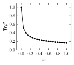
(a) Stochastic case

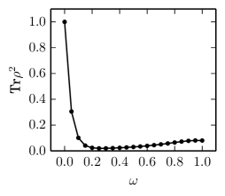
(b) Classical case

Figure 1. Purity of final state for stochastic walk on a line segment of length 400, with time 25 and the initial state is $|200\rangle\langle 200|$.

Analyzing Fig. 1 one can see that the purity in the global dissipation case, decreases rapidly with $\omega$, and has sharp maximum at $\omega=0$. The conclusion is that, if the ballistic regime, $\alpha=2$, is sustained for strong environment interaction, $\omega\rightarrow 1$, it is not caused by a high purity.

4. The asymptotic scaling exponent approach

In this section we investigate the asymptotic scaling of the second central moment of the frequency distribution of the walker position [26, 27, 28].

Remark 6.

The asymptotic scaling exponent distinguishes between different types of diffusion process [17, 18, 19, 20]:

• if $\alpha<1$ the process is sub-diffusive,

• if $\alpha=1$ the process obeys a normal diffusion regime,

• if $1<\alpha<2$ the process is super-diffusive,

• if $\alpha=2$ the process obeys a ballistic diffusion regime.

For the standard Markovian random walk on a uniform lattice the asymptotic scaling exponent value is $\alpha=1$ [28]. For the quantum walk on such a lattice it is $\alpha=2$ [29].

Consider now the general stochastic walk which is a combination of the quantum walk, where $\alpha=2$, and purely dissipative stochastic walk, where $\alpha=1$ no matter which of the studied dissipation operators are chosen. We use the asymptotic scaling exponent to evaluate which regime, classical or quantum, dominates the process for $\omega\in(0,1)$.

Let us discuss now the procedure used to calculate the asymptotic scaling exponent. The second moment of the probability distribution of the stochastic walk at time $t$ is given by

(27) $$\mu_{2}(t)=\sum_{k}k^{2}\langle k|\rho(t)|k\rangle.$$

To compute the asymptotic scaling exponent we use the standard scaling relation  [17, 18, 19, 20, 27]

(28) $$\mu_{2}(t)\propto t^{\alpha},$$

We have the following results regarding the moments of the stochastic walk. First, we calculate the $m$^th central moment for a stochastic walk on a line.

Proposition 7.

For a stochastic walk on a line with an initial state $\rho(0)=|0\rangle\langle 0|$, $\omega=1$ and $L_{S}$ as in Eq (7), the $m$-th central moment $\mu_{m}(t)$ is polynomial in $t$ for $m$ even and zero otherwise. Moreover for even $m$ we have

(29) $$\lim_{t\to\infty}\frac{\mu_{m}(t)}{t^{\frac{m}{2}}}=\frac{m!}{\left(\frac{m}{2}\right)!8^{\frac{m}{2}}}\binom{m}{\frac{m}{2}}.$$

The proof of Proposition 7 is given in Appendix B. From this, we get that the second central moment has the form $\mu_{2}(t)=\frac{1}{2}t$.

Now, we move to the case of arbitrary non-zero $\omega$. We study the leading term in the $m$^th central moment.

Proposition 8.

For a stochastic walk on a line with an initial state $\rho(0)=|0\rangle\langle 0|$ and $\omega\in(0,1)$, the $m$-th central moment $\mu_{m}(t)$ is polynomial in $t$ for even $m$ and zero otherwise. Moreover for even $m$ we have

(30) $$\lim_{t\to\infty}\frac{\mu_{m}(t)}{t^{m}}=\binom{m}{\frac{m}{2}}(\omega-1)^{m}.$$

Now, we calculate the second central moment. We get the following result.

Proposition 9.

For a stochastic walk on a line with an initial state $\rho(0)=|0\rangle\langle 0|$ and $\omega\in(0,1]$ the second central moment is of the form

(31) $$\mu_{2}(t)=2\left(\omega-1\right)^{2}t^{2}+\frac{\omega}{2}t.$$

Proofs of Propositions 8 and 9 are given in Appendix C.

From these propositions, we get that the asymptotic scaling exponent in the case of the Lindblad operator as in Eq (7) is:

1. if $\omega\neq 1$ (general stochastic walk case) we have $\alpha=2$,

2. if $\omega=1$ (purely dissipative case) we have $\alpha=1.$

At first glance, this results seems to be quite surprising as the walk exhibits ballistic behavior as long as we have a finite amount of a coherent evolution. This effect can be explained as follows. If we have $\omega<1$, then the quantum effects dominate the system, despite the measurement. However, if we turn off the coherent evolution, then we get a behavior determined only by the random disturbances of the system due to the measurement. In this case we get a behavior resembling a classical random walk in the sense that $\alpha=1$.

On the other, when we consider the local dissipation, we get the opposite result. In this case we get that $\alpha=2$ if $\omega=0$ and $\alpha<2$ if $\omega>0$. This can be explained easily. As stated in the introduction, the Lindblad terms in this case introduce energy damping to the evolution of the system. If we have a system driven by a Hamiltonian $H$ and perform a continuous energy damping on it, then for large times $t$, the system becomes completely classical.

5. Conclusions

In this work we studied the behavior of quantum stochastic walks on a line and a line segments. We found an analytical formula for the probability distribution of the walk in the case of a global dissipation operator, equivalent to a continuous position measurement. To measure the quantum coherence of the walk, we used the asymptotic approach. Hence we investigated the scaling of the second moment of the frequency distribution, by means of the asymptotic scaling exponent, $\alpha$. There are other known approaches to quantifying quantumness in a quantum walk model. One of the is the amount of needed corrections to the classical stationary state of the walk to recover a time averaged quantum distribution [30]. The main difference between this result and ours is the fact that our result applies to arbitrary initial state, whereas the result from [30] requires that the initial state is mostly in the ground space of the walk’s Hamiltonian.

In the case of the stochastic walk on a line, with the global dissipation operator the ballistic propagation was demonstrated, since for large walk time, the relation $\alpha=2$ holds. Importantly, such ballistic propagation occurs for each strength of the dissipation as long as the Hamiltonian term is present in the master equation. This result is surprising and in contrary to the asymptotic behavior of the stochastic walk with local dissipation, equivalent to continuous energy damping. In such case even small dissipation leads to the classical propagation of the walk and $\alpha=1$ for large time of the walk.

If we analyze the asymptotic behavior, the global dissipation leads to a quantum-like propagation. This result is interesting while constructing quantum system that is supposed to keep the coherence regardless of an environmental interaction. Such observation may be useful in a quantum computer development, where maintaining quantum coherence is crucial.

Appendix A Proof of Proposition 2

First, we will need a couple of technical lemmas:

Lemma 10 ([31]).

For arbitrary $n\in\mathbb{N}$ and $x\in\mathbb{R}$ such that $x\neq\frac{k\pi}{2}$ for $k\in\mathbb{Z}$

(32) $$\sum_{i=1}^{n}\sin^{4}(ix)=\frac{1}{8}\left(3n-4\frac{\cos\left((n+1)x\right)\sin(nx)}{\sin(x)}+\frac{\cos\left(2(n+1)x\right)\sin(2nx)}{\sin(2x)}\right).$$

Lemma 11 ([31]).

For arbitrary $n\in\mathbb{N}$ and $x\in\mathbb{R}$ such that $x\neq 2k\pi$ for $k\in\mathbb{Z}$

(33) $$\sum_{h=1}^{n}\cos(hx)=\frac{1}{2}\left(\frac{\sin\left(\frac{2n+1}{2}x\right)}{\sin\left(\frac{x}{2}\right)}-1\right).$$

Now, we are ready to prove Proposition 2

Proof of Proposition 2.

By Theorem 1 we have

(34) $$\lim_{t\to\infty}\rho_{kk}=\left(\frac{2}{n+1}\right)^{2}\sum_{i=1}^{n}\sin^{2}\left(\frac{ki\pi}{n+1}\right)\sin^{2}\left(\frac{li\pi}{n+1}\right).$$

Now we analyze the sum above. Suppose $k=l$. Then we have

(35) $$\rho_{kk}=\left(\frac{2}{n+1}\right)^{2}\sum_{i=1}^{n}\sin^{4}\left(\frac{ik\pi}{n+1}\right).$$

Suppose $k\neq\frac{n+1}{2}$. By Lemma 10 the sum above equals

(36) $$\begin{split}\rho_{kk}&=\left(\frac{2}{n+1}\right)^{2}\frac{1}{8}\left(3n-4\frac{\cos(\pi k)\sin\left(\frac{n\pi k}{n+1}\right)}{\sin\left(\frac{\pi k}{n+1}\right)}+\frac{\cos(2\pi k)\sin\left(\frac{2\pi nk}{n+1}\right)}{\sin\left(\frac{2\pi k}{n+1}\right)}\right)\\ &=\left(\frac{2}{n+1}\right)^{2}\frac{1}{8}\left(3n+4(-1)^{k}(-1)^{k}\frac{\sin\left(\frac{\pi k}{n+1}\right)}{\sin\left(\frac{\pi k}{n+1}\right)}-\frac{\sin\left(\frac{2\pi k}{n+1}\right)}{\sin\left(\frac{2\pi k}{n+1}\right)}\right)\\ &=\left(\frac{2}{n+1}\right)^{2}\frac{1}{8}(3n+4-1)=\frac{3}{2(n+1)},\end{split}$$

since $\cos(k\pi)=(-1)^{k}$ and $\sin\frac{nk\pi}{n+1}=-(-1)^{k}\sin\frac{\pi k}{n+1}$ and similarly for second formula. Now suppose $k=\frac{n+1}{2}$. Then

(37) $$\begin{split}\rho_{kk}&=\left(\frac{2}{n+1}\right)^{2}\sum_{i=1}^{n}\sin^{4}\left(\frac{ik\pi}{n+1}\right)=\left(\frac{2}{n+1}\right)^{2}\sum_{i=1}^{n}\sin^{4}\left(\frac{i\pi}{2}\right)\\ &=\left(\frac{2}{n+1}\right)^{2}\frac{2n+1+(-1)^{n+1}}{4}=\left(\frac{2}{n+1}\right)^{2}\frac{n+1}{2}=\frac{2}{n+1},\\ \end{split}$$

since $l=\frac{n+1}{2}$ implies $n+1$ is even.

Suppose we have $k+l=n+1$. Then

(38) $$\begin{split}\rho_{kk}&=\left(\frac{2}{n+1}\right)^{2}\sum_{i=1}^{n}\sin^{2}\left(\frac{(n+1-k)i\pi}{n+1}\right)\sin^{2}\left(\frac{ik\pi}{n+1}\right)\\ &=\left(\frac{2}{n+1}\right)^{2}\sum_{i=1}^{n}\sin^{4}\left(\frac{ik\pi}{n+1}\right)=\frac{3}{2(n+1)}.\end{split}$$

Suppose now that $k\neq l$ and $k\neq n+1-l$. Then by formula

(39) $$\sin^{2}(x)\sin^{2}(y)=\frac{1}{8}(\cos(2x-2y)+\cos(2x+2y)-2\cos(2x)-2\cos(2y)+2)$$

and by Lemma 11 we have

(40) $$\begin{split}\rho_{kk}&=\left(\frac{2}{n+1}\right)^{2}\frac{1}{16}\left(2+4n-2\frac{\sin\left(\frac{l(2n+1)\pi}{n+1}\right)}{\sin\left(\frac{l\pi}{n+1}\right)}+\frac{\sin\left(\frac{(k-l)(2n+1)\pi}{n+1}\right)}{\sin\left(\frac{(k-l)\pi}{n+1}\right)}\right.\\ &\phantom{=\ }+\left.\frac{\sin\left(\frac{(k+l)(2n+1)\pi}{n+1}\right)}{\sin\left(\frac{(k+l)\pi}{n+1}\right)}-2\frac{\sin\left(\frac{k(2n+1)\pi}{n+1}\right)}{\sin\left(\frac{k\pi}{n+1}\right)}\right)\\ &=\frac{1}{4(n+1)^{2}}\left(2+4n+2\frac{\sin\left(\frac{l\pi}{n+1}\right)}{\sin\left(\frac{l\pi}{n+1}\right)}-\frac{\sin\left(\frac{(k-l)\pi}{n+1}\right)}{\sin\left(\frac{(k-l)\pi}{n+1}\right)}-\frac{\sin\left(\frac{(k+l)\pi}{n+1}\right)}{\sin\left(\frac{(k+l)\pi}{n+1}\right)}+2\frac{\sin\left(\frac{k\pi}{n+1}\right)}{\sin\left(\frac{k\pi}{n+1}\right)}\right)\\ &=\frac{4(n+1)}{4(n+1)^{2}}=\frac{1}{n+1}.\end{split}$$

∎

Appendix B Proof of Proposition 7

First we need a couple of technical lemmas:

Lemma 12 ([31]).

For arbitrary $\alpha\in\mathbb{R}$, $n,m\in\mathbb{N}$ such that $m\leq n$ we have

(41) $$\sum_{k=0}^{n}(-1)^{k}(k-\alpha)^{m}\binom{n}{k}=\begin{cases}0,&m<n,\\ (-1)^{n}n!&m=n.\end{cases}$$

Lemma 13 ([31]).

For arbitrary $n,p\in\mathbb{N}$ such that $p\leq n$ we have

(42) $$\sum_{k=0}^{n-p}\binom{n}{k}\binom{n}{p+k}=\binom{2n}{n-p}.$$

Lemma 14.

For arbitrary $k,l\in\mathbb{N}$ we have

(43) $$\int_{-\pi}^{\pi}\cos(kx)\left[\cos(x)\right]^{l}\mathrm{d}x=\begin{cases}\frac{2\pi}{2^{l-k}}\binom{l-k}{\frac{l-k}{2}}\prod_{i=0}^{k-1}\frac{l-i}{l+k-2i},&l\geq k\textrm{ and }l=k\mod 2,\\ 0,&\textrm{otherwise.}\\ \end{cases}$$

Proof.

Using the formula [31]

(44) $$\int\left[\cos(x)\right]^{l}\cos(kx)\mathrm{d}x=\frac{1}{l+k}\left[\left(\cos(x\right))^{l}\sin(kx)+l\int\left[\cos(x)\right]^{l-1}\cos((k-1)x)\mathrm{d}x\right]$$

we obtain

(45) $$\int_{-\pi}^{\pi}\left[\cos(x)\right]^{l}\cos(kx)\mathrm{d}x=\frac{l}{l+k}\int_{-\pi}^{\pi}\left[\cos(x)\right]^{l-1}\cos((k-1)x)\mathrm{d}x.$$

Moreover for arbitrary $l\in\mathbb{N}$ we have [31]

(46) $$\int\left[\cos(x)\right]^{2l}\mathrm{d}x=\frac{1}{4^{l}}\binom{2l}{l}x+\frac{2}{4^{l}}\sum_{k=0}^{l-1}\binom{2l}{k}\frac{\sin((2l-2k)x)}{2l-2k},$$

which provides us the formula

(47) $$\int_{-\pi}^{\pi}\left[\cos(x)\right]^{2l}\mathrm{d}x=\frac{2\pi}{4^{l}}\binom{2l}{l}.$$

Suppose $l<k$. Then using Eq. (45) we have

(48) $$\int_{-\pi}^{\pi}\left[\cos(x)\right]^{l}\cos(kx)\mathrm{d}x=\prod_{i=0}^{l-1}\frac{l-i}{l+k-2i}\int_{-\pi}^{\pi}\cos((k-l)x)\mathrm{d}x=0.$$

If $l\geq k$, then we obtain

(49) $$\int_{-\pi}^{\pi}\left[\cos(x)\right]^{l}\cos(kx)=\prod_{i=0}^{k-1}\frac{l-i}{l+k-2i}\int_{-\pi}^{\pi}\cos^{l-k}(x)\mathrm{d}x.$$

If $l-k$ is odd, then the integral equals 0. Otherwise using Eq. (47) we have

(50) $$\int_{-\pi}^{\pi}\cos(kx)\cos^{l}(x)=\frac{2\pi}{2^{l-k}}\binom{l-k}{\frac{l-k}{2}}\prod_{i=0}^{k-1}\frac{l-i}{l+k-2i}.$$

∎

Proposition 15.

For a stochastic walk on a line with an initial state $\rho(0)=|0\rangle\langle 0|$ and $\omega=1$, the $\rho_{kk}(t)$ has series representation with respect to $t$ of the form

(51) $$\rho_{kk}(t)=\sum_{n=|k|}^{\infty}\frac{(-1)^{n+k}}{8^{n}}\binom{2n}{n}\binom{2n}{n+k}\frac{t^{n}}{n!}.$$

Proof.

Since the elements $\rho_{kk}(t)$ are symmetric with respect to $k=0$, we assume $k\geq 0$. By Theorem 3 we have

(52) $$\rho_{kk}(t)=\frac{1}{4\pi^{2}}\int_{-\pi}^{\pi}\int_{-\pi}^{\pi}\cos(kx)\cos(ky)\exp\left[-\frac{t}{2}(\cos(x)-\cos(y))^{2}\right]\mathrm{d}x\mathrm{d}y.$$

Suppose we have the Taylor series representation $\rho_{kk}(t)=\sum_{n=0}^{\infty}\frac{A_{n,k}}{n!}t^{n}$. Then $A_{n,k}$ is of the form

(53) $$\begin{split}A_{n,k}&=\frac{(-1)^{n}}{4\cdot 2^{n}\pi^{2}}\int_{-\pi}^{\pi}\int_{-\pi}^{\pi}\cos(kx)\cos(ky)\left(\cos(x)-\cos(y)\right)^{2n}\mathrm{d}x\mathrm{d}y\\ &=\frac{(-1)^{n}}{4\cdot 2^{n}\pi^{2}}\sum_{l=0}^{2n}\binom{2n}{l}(-1)^{l}\int_{-\pi}^{\pi}\cos(kx)\left[\cos(x)\right]^{l}\mathrm{d}x\int_{-\pi}^{\pi}\cos(ky)\left[\cos(y)\right]^{2n-l}\mathrm{d}y.\end{split}$$

Let us define for simplicity

(54) $$A_{n,k,l}=\binom{2n}{l}(-1)^{l}\int_{-\pi}^{\pi}\cos(kx)\left[\cos(x)\right]^{l}\mathrm{d}x\int_{-\pi}^{\pi}\cos(ky)\left[\cos(y)\right]^{2n-l}\mathrm{d}y.$$

By Lemma 14 we have that $A_{n,k,l}$ is non-zero when $k-l$ is even and has the form

(55) $$A_{n,k,l}=\frac{(-1)^{l}4\pi^{2}}{2^{2n-2k}}\binom{2n}{l}\binom{l-k}{\frac{l-k}{2}}\binom{2n-l-k}{n-\frac{l+k}{2}}\prod_{i=0}^{k-1}\frac{l-i}{l+k-2i}\frac{2n-l-i}{2n-l+k-2i}.$$

In particular, we note that for $n<k$ we have $A_{n,k}=0$.

Again it is straightforward to find

(56) $$A_{n,k,k}=\frac{(-1)^{k}4\pi^{2}}{4^{n}}\binom{2n}{n}\binom{n}{k}$$

and

(57) $$\frac{A_{n,k,l+2}}{A_{n,k,l}}=\frac{(n-\frac{l-k}{2})(n-\frac{l-k}{2})}{(\frac{l+k}{2}+1)(\frac{l-k}{2}+1)}.$$

Note that we increment $l$ by two instead of one because of the assumption that $l-k$ is even. One can verify, that the $A_{n,k,l}$ is of the form

(58) $$A_{n,k,l}=\frac{(-1)^{k}4\pi^{2}}{4^{n}}\binom{2n}{n}\binom{n}{\frac{l+k}{2}}\binom{n}{\frac{l-k}{2}},$$

and hence have

(59) $$\begin{split}A_{n,k}&=\frac{(-1)^{n}}{4\cdot 2^{n}\pi^{2}}\sum_{l\in\{k,k+2,\dots,2n-k\}}A_{n,k,l}\\ &=\frac{(-1)^{n+k}}{8^{n}}\binom{2n}{n}\sum_{l\in\{k,k+2,\dots,2n-k\}}\binom{n}{\frac{l+k}{2}}\binom{n}{\frac{l-k}{2}}\\ &=\frac{(-1)^{n+k}}{8^{n}}\binom{2n}{n}\sum_{l=0}^{n-k}\binom{n}{l+k}\binom{n}{l}\\ &=\frac{(-1)^{n+k}}{8^{n}}\binom{2n}{n}\binom{2n}{n+k},\end{split}$$

where in the third line we change the indices range and in the last line we use Lemma 13. ∎

Now we are ready to prove Proposition 7.

Proof of Proposition 7.

Note that odd moments equals 0 by symmetry of the probability distribution. Suppose $m$ is even and $m>0$. Then by Proposition 15 we have

(60) $$\begin{split}\mu_{m}(t)&=\sum_{k=-\infty}^{\infty}k^{m}\sum_{n=|k|}^{\infty}\frac{(-1)^{n+k}}{8^{n}}\binom{2n}{n}\binom{2n}{n+k}\frac{t^{n}}{n!}\\ &=\sum_{n=0}^{\infty}\frac{(-1)^{n}}{8^{n}}\binom{2n}{n}\frac{t^{n}}{n!}\sum_{k=-n}^{n}k^{m}(-1)^{k}\binom{2n}{n+k}\\ &=\sum_{n=0}^{\infty}\frac{1}{8^{n}}\binom{2n}{n}\frac{t^{n}}{n!}\sum_{k=0}^{2n}(k-n)^{m}(-1)^{k}\binom{2n}{k}.\end{split}$$

By Lemma 12 formula above can be simplified

(61) $$\mu_{m}(t)=\sum_{n=1}^{\frac{m}{2}}\frac{1}{8^{n}}\binom{2n}{n}\frac{t^{n}}{n!}\sum_{k=0}^{2n}(k-n)^{m}(-1)^{k}\binom{2n}{k},$$

hence the $m$-th central moment is a polynomial of degree $\frac{m}{2}$ with respect to $t$. Moreover, the coefficient next to $t^{\frac{m}{2}}$ is

(62) $$a_{\frac{m}{2}}=\frac{m!}{\left(\frac{m}{2}\right)!8^{\frac{m}{2}}}\binom{m}{\frac{m}{2}}.$$

∎

Appendix C Proof of Propositions 8 and 9

proof of Proposition 8.

Case $\omega=1$ was already considered in Theorem 7. Suppose $\omega\in(0,1)$. As in Appendix B, we start by finding the Taylor series representation for the probability distribution. If we denote $\rho_{kk}(t)=\sum_{n=0}^{\infty}\frac{B_{n,k}}{n!}t^{n}$, then one can find that $B_{n,k}$ is of the form

(63) $$\begin{split}B_{n,k}&=\sum_{l=0}^{n}\binom{n}{l}\frac{1}{4\pi^{2}}\int_{-\pi}^{\pi}\int_{-\pi}^{\pi}\cos(kx)\cos(ky)\frac{(-\omega)^{n-l}}{2^{n-l}}\times\\ &\phantom{\ =}\times(\cos(x)-\cos(y))^{2n-l}2^{l}\mathrm{i}^{l}(1-\omega)^{l}\mathrm{d}x\mathrm{d}y.\end{split}$$

Since $\rho_{kk}(t)\in\mathbb{R}$, we can exclude the imaginary terms and we can simplify the formula

(64) $$\begin{split}B_{n,k}&=\sum_{l=0}^{\lfloor\frac{n}{2}\rfloor}\binom{n}{2l}8^{l}\omega^{n-2l}(1-\omega)^{2l}\times\\ &\phantom{\ =}\times\frac{(-1)^{n-l}}{2^{n-l}4\pi^{2}}\int_{-\pi}^{\pi}\int_{-\pi}^{\pi}\cos(kx)\cos(ky)(\cos(x)-\cos(y))^{2n-2l}\mathrm{d}x\mathrm{d}y\\ &=\sum_{l=0}^{\lfloor\frac{n}{2}\rfloor}\binom{n}{2l}8^{l}\omega^{n-2l}(1-\omega)^{2l}A_{n-l,k}.\end{split}$$

From Appendix B we know, that $A_{n,k}$ is of the form

(65) $$A_{n,k}=\begin{cases}0,&|k|>n,\\ \frac{(-1)^{n+k}}{8^{n}}\binom{2n}{n}\binom{2n}{n+k},&|k|\leq n.\end{cases}$$

In our case we have the condition $|k|\leq n-\frac{l}{2}\leq n$. Hence we conclude, that $B_{n,k}$ is of the form

(66) $$B_{n,k}=\frac{(-1)^{n+k}}{8^{n}}\sum_{l=0}^{\min(\lfloor\frac{n}{2}\rfloor,n-|k|)}\binom{n}{2l}8^{2l}\omega^{n-2l}(1-\omega)^{2l}(-1)^{l}\binom{2n-2l}{n-l}\binom{2n-2l}{n-l+k}.$$

Therefore for even $m$ we have

(67) $$\begin{split}\mu_{m}(t)&=\sum_{k=-\infty}^{\infty}k^{m}\sum_{n=0}^{\infty}B_{n,k}\frac{t^{n}}{n!}\\ &=\sum_{n=0}^{\infty}\frac{t^{n}}{n!}\sum_{k=-n}^{n}k^{m}B_{n,k}\\ &=\sum_{n=0}^{\infty}\frac{(-1)^{n}t^{n}}{8^{n}n!}\sum_{k=-n}^{n}k^{m}(-1)^{k}\sum_{l=0}^{\min(\lfloor\frac{n}{2}\rfloor,n-|k|)}\binom{n}{2l}8^{2l}\omega^{n-2l}(1-\omega)^{2l}(-1)^{l}\binom{2n-2l}{n-l}\binom{2n-2l}{n-l+k}\\ &=\sum_{n=0}^{\infty}\sum_{k=-n}^{n}\sum_{l=0}^{\min(\lfloor\frac{n}{2}\rfloor,n-|k|)}C_{n,l,t}\omega^{n-2l}(1-\omega)^{2l}(-1)^{k}k^{m}\binom{2n-2l}{n-l+k},\\ &=\sum_{n=0}^{\infty}\sum_{l=0}^{\lfloor\frac{n}{2}\rfloor}C_{n,l,t}\omega^{n-2l}(1-\omega)^{2l}\sum_{k=-(n-l)}^{n-l}(-1)^{k}k^{m}\binom{2n-2l}{n-l+k},\\ &=\sum_{n=0}^{\infty}\sum_{l=0}^{\lfloor\frac{n}{2}\rfloor}C_{n,l,t}\omega^{n-2l}(1-\omega)^{2l}(-1)^{n-l}\sum_{k=0}^{2n-2l}(-1)^{k}(k-(n-l))^{m}\binom{2n-2l}{k},\\ \end{split}$$

where

(68) $$C_{n,t,l}=\frac{(-1)^{n}t^{n}}{8^{n}n!}8^{2l}(-1)^{l}\binom{n}{2l}\binom{2n-2l}{n-l}.$$

Let us denote

(69) $$\alpha_{2n-2l,m}=\sum_{k=0}^{2n-2l}(-1)^{k}(k-(n-l))^{m}\binom{2n-2l}{k}.$$

From Lemma 12 $\alpha_{2n-2l,m}$ is nonzero if $m\geq 2n-2l\iff l\geq n-\frac{m}{2}$. Hence Eq. (67) can be simplified

(70) $$\begin{split}\mu_{m}(t)=\sum_{n=0}^{\infty}\sum_{l=n-\frac{m}{2}}^{\lfloor\frac{n}{2}\rfloor}C_{n,l,t}(-1)^{n-l}\omega^{n-2l}(1-\omega)^{2l}\alpha_{2n-2l,m}\end{split}$$

The condition $n-\frac{m}{2}\leq l\leq\lfloor\frac{n}{2}\rfloor$ implies $0\leq n\leq m$. Hence, we have

(71) $$\begin{split}\mu_{m}(t)&=\sum_{n=0}^{m}\sum_{l=n-\frac{m}{2}}^{\lfloor\frac{n}{2}\rfloor}C_{n,l,t}(-1)^{n-l}\omega^{n-2l}(1-\omega)^{2l}\alpha_{2n-2l,m}\\ &=\sum_{n=0}^{m}\sum_{l=n-\frac{m}{2}}^{\lfloor\frac{n}{2}\rfloor}\frac{(-1)^{n}t^{n}}{8^{n}n!}8^{2l}(-1)^{n}\binom{n}{2l}\binom{2n-2l}{n-l}\omega^{n-2l}(1-\omega)^{2l}\alpha_{2n-2l,m}\\ &=\sum_{n=0}^{m}\beta_{n,\omega}t^{n}.\end{split}$$

Let us calculate the leading term, $\beta_{m,\omega}$. Then we have $l\in\{\frac{m}{2}\}$ and $n=m$ and $m$ is even.

(72) $$\begin{split}\beta_{m}&=\sum_{l=m-\frac{m}{2}}^{\lfloor\frac{m}{2}\rfloor}\frac{(-1)^{m}}{8^{m}m!}8^{2l}(-1)^{m}\binom{m}{2l}\binom{2m-2l}{m-l}\omega^{m-2l}(1-\omega)^{2l}\alpha_{2m-2l,m}\\ &=\frac{1}{8^{m}m!}8^{m}\binom{m}{m}\binom{m}{\frac{m}{2}}(1-\omega)^{m}\alpha_{m,m}\\ &=\frac{1}{m!}\binom{m}{\frac{m}{2}}(1-\omega)^{m}(-1)^{m}m!=\binom{m}{\frac{m}{2}}(1-\omega)^{m},\end{split}$$

where we used the fact, that $\alpha_{m,m}=(-1)^{m}m!$ by Lemma 12. ∎

References

• [1] A. Gonis and P. E. Turchi, Decoherence and its implications in quantum computation and information transfer, vol. 182. IOS press, 2001.
• [2] M. H. Amin, D. V. Averin, and J. A. Nesteroff, “Decoherence in adiabatic quantum computation,” Physical Review A, vol. 79, no. 2, p. 022107, 2009.
• [3] A. Kossakowski, “On quantum statistical mechanics of non-hamiltonian systems,” Reports on Mathematical Physics, vol. 3, no. 4, pp. 247–274, 1972.
• [4] G. Lindblad, “On the generators of quantum dynamical semigroups,” Communications in Mathematical Physics, vol. 48, no. 2, pp. 119–130, 1976.
• [5] V. Gorini, A. Kossakowski, and E. C. G. Sudarshan, “Completely positive dynamical semigroups of n-level systems,” Journal of Mathematical Physics, vol. 17, no. 5, pp. 821–825, 1976.
• [6] J. D. Whitfield, C. A. Rodríguez-Rosario, and A. Aspuru-Guzik, “Quantum stochastic walks: A generalization of classical random walks and quantum walks,” Physical Review A, vol. 81, no. 2, p. 022323, 2010.
• [7] S. E. Venegas-Andraca, “Quantum walks: a comprehensive review,” Quantum Information Processing, vol. 11, no. 5, pp. 1015–1106, 2012.
• [8] C. Robens, W. Alt, D. Meschede, C. Emary, and A. Alberti, “Ideal negative measurements in quantum walks disprove theories based on classical trajectories,” Physical Review X, vol. 5, no. 1, p. 011003, 2015.
• [9] M. Stefanak, “Interference phenomena in quantum information,” arXiv preprint arXiv:1009.0200, 2010.
• [10] R. Vieira, E. P. Amorim, and G. Rigolin, “Dynamically disordered quantum walk as a maximal entanglement generator,” Physical review letters, vol. 111, no. 18, p. 180503, 2013.
• [11] P. Kurzyński and A. Wójcik, “Quantum walk as a generalized measuring device,” Physical review letters, vol. 110, no. 20, p. 200404, 2013.
• [12] B. Kollár and M. Koniorczyk, “Entropy rate of message sources driven by quantum walks,” Physical Review A, vol. 89, no. 2, p. 022338, 2014.
• [13] T. Kitagawa, M. S. Rudner, E. Berg, and E. Demler, “Exploring topological phases with quantum walks,” Physical Review A, vol. 82, no. 3, p. 033429, 2010.
• [14] P. Arnault and F. Debbasch, “Quantum walks and discrete gauge theories,” Physical Review A, vol. 93, no. 5, p. 052301, 2016.
• [15] C. Chandrashekar, S. Banerjee, and R. Srikanth, “Relationship between quantum walks and relativistic quantum mechanics,” Physical Review A, vol. 81, no. 6, p. 062340, 2010.
• [16] A. Chia, A. Górecka, T. K. C, Ł. Pawela, K. P, T. Paterek, and D. Kaszlikowski, “Coherent chemical kinetics as quantum walks i: Reaction operators for radical pairs,” Physical Review E, vol. 93, p. 032407, 2016.
• [17] R. Metzler, J.-H. Jeon, A. G. Cherstvy, and E. Barkai, “Anomalous diffusion models and their properties: non-stationarity, non-ergodicity, and ageing at the centenary of single particle tracking,” Physical Chemistry Chemical Physics, vol. 16, no. 44, pp. 24128–24164, 2014.
• [18] J. Spiechowicz, J. Łuczka, and P. Hänggi, “Transient anomalous diffusion in periodic systems: ergodicity, symmetry breaking and velocity relaxation,” Scientific Reports, vol. 6, 2016.
• [19] J. Spiechowicz and J. Łuczka, “Diffusion anomalies in ac-driven brownian ratchets,” Physical Review E, vol. 91, no. 6, p. 062104, 2015.
• [20] R. Klages, G. Radons, and I. M. Sokolov, Anomalous transport: foundations and applications. John Wiley & Sons, 2008.
• [21] J. Kempe, “Quantum random walks: an introductory overview,” Contemporary Physics, vol. 44, no. 4, pp. 307–327, 2003.
• [22] A. O. Caldeira and A. J. Leggett, “Path integral approach to quantum brownian motion,” Physica A: Statistical mechanics and its Applications, vol. 121, no. 3, pp. 587–616, 1983.
• [23] N. Prokof’ev and P. Stamp, “Decoherence and quantum walks: Anomalous diffusion and ballistic tails,” Physical Review A, vol. 74, no. 2, p. 020102, 2006.
• [24] K. Jacobs and D. A. Steck, “A straightforward introduction to continuous quantum measurement,” Contemporary Physics, vol. 47, no. 5, pp. 279–303, 2006.
• [25] S. Noschese, L. Pasquini, and L. Reichel, “Tridiagonal toeplitz matrices: properties and novel applications,” Numerical linear algebra with applications, vol. 20, no. 2, pp. 302–326, 2013.
• [26] S. Havlin and D. Ben-Avraham, “Fractal dimensionality of polymer chains,” Journal of Physics A: Mathematical and General, vol. 15, no. 6, p. L311, 1982.
• [27] J. Haus and K. Kehr, “Diffusion in regular and disordered lattices,” Physics Reports, vol. 150, no. 5, pp. 263–406, 1987.
• [28] S. Havlin and D. Ben-Avraham, “Diffusion in disordered media,” Advances in Physics, vol. 36, no. 6, pp. 695–798, 1987.
• [29] G. Grimmett, S. Janson, and P. F. Scudo, “Weak limits for quantum random walks,” Physical Review E, vol. 69, no. 2, p. 026119, 2004.
• [30] M. Faccin, T. Johnson, J. Biamonte, S. Kais, and P. Migdał, “Degree distribution in quantum walks on complex networks,” Physical Review X, vol. 3, no. 4, p. 041007, 2013.
• [31] I. S. Gradshteyn and I. M. Ryzhik, Table of integrals, series, and products. Academic press, 2014.