FAST-SLOW VECTOR FIELDS OF REACTION-DIFFUSION SYSTEMS

Abstract.

A geometrically invariant concept of fast-slow vector fields perturbed by transport terms (describing molecular diffusion) is proposed in this paper. It is an extension of our concept of singularly perturbed vector fields to reaction-diffusion systems. This paper is motivated by an algorithm of reaction-diffusion manifolds (REDIM). It can be considered as its theoretical justification extending it from a practical algorithm to a robust computational method. Fast-slow vector fields can be represented locally as "singularly perturbed systems of PDE". The paper focuses on development of the decomposition to a fast and slow subsystems. It is demonstrated that transport terms can be neglected (under reasonable physical assumptions) for the fast subsystem. A simple practical application example of the proposed algorithm for numerical treatment of reaction-diffusion systems is demonstrated.

1. Introduction

The decomposition of complex dynamical systems into simpler subsystems using different rates of changes (multiple time scales) for different subsystems is common in physical and engineering models [17]-[19]. The main difficulty in applications is a "hidden", implicit form of the decomposition of the system evolving at different time scales. Namely, there is no explicit representation of the system in relatively fast and slow subsystems available.

A formal mathematical basis to cope with this problem is based on the notion of singularly perturbed vector fields [5]. Let us briefly introduce some key ideas of the singularly perturbed vector fields (SPVFs) that can be used to treat the problem of the decomposition in general.

Roughly speaking a singularly perturbed vector field (SPVF) $F(z,\varepsilon)$ is a vector field defined in a domain $G$ of Euclidian space $R^{n}$ that depends on a small parameter $\varepsilon\geq 0$ such that for any point $z$, $F(z,0)$ belongs to an a priori fixed fast subspace $M_{f}(z)$ of smaller dimension - $\dim M_{f}(z)<n$. Moreover, the dimension of $M_{f}(z)$ does not depend on the choice of the point $z$. Thus, in this case the vector field $F(z,\varepsilon)$ can be decomposed into a fast sub-field that belongs to the fast subspace $M_{f}(z)$ and its complement representing a slow sub-field. Of course this is not a formal description, which is more sophisticated. Additionally, if $M_{f}(z)$ does not depend on $x$ then the vector field $F(z,\varepsilon)$ represents (by definition) a linearly decomposed singularly perturbed vector field. Accordingly, the notion of the linearly decomposed singularly perturbed vector field is a geometrical analog of a singularly perturbed system.

A formal concept (a theory of SPVFs) can be useful for practical applications if it is supported by an identification algorithm for these fast sub-fields [7]. In a number of previous papers an algorithm for linearly decomposed singularly perturbed vector fields [3] has been constructed. This algorithm is based on a global linear interpolation procedure for an original vector field that we call a Global Quasi-Linearization (GQL) (see e.g. [7, 3]).

The theory of singularly perturbed vector fields is a coordinate free version of singularly perturbed systems for (ODEs) [10] - [20]. It cannot be used in the original form for study the influence of transport processes of reaction-diffusion systems. Thus, the main formal object of our current study should be modified as

$$\mathrm{F}(z,x,\varepsilon):=\Phi(z,\varepsilon)+L(z,x,\varepsilon).$$

It combines a singularly perturbed vector field $\Phi(z,\varepsilon)$ (reaction term) and a linear operator typically of second order (diffusion term). Here $x$ belongs to a set $V_{s}$ in Euclidian space $R^{s},s\leq 3$. Typically it is a segment $[0,L]$ or closed parallelogram. Additionally, fast reaction terms are assumed to be much faster than corresponding transport processes, that leads to a formal assumption $\lim_{\varepsilon\to 0}L(z,x,\varepsilon)=0$, i.e. $\mathrm{F}(z,x,0)=\Phi(z,0)$. This makes the extension of the theoretical framework developed in [5, 7] straightforward.

2. General formal Notion of Fast-Slow Vector Fields

In this section, the main formal framework of singularly perturbed vector fields [5] to fast-slow vector fields of reaction-diffusion systems is adopted.

As in previous, a standard definition of vector bundles and use vector/fiber bundles as a formal substitute for so-called nonlinear coordinate systems.

Definition.

A vector bundle $\xi$ over a connected manifold $N\subset R^{m}$ consists of a set $E\subset R^{m}$ (the total set), a smooth map $p:E\rightarrow N$ (the projection) which is onto, and each fiber $F_{x}^{\xi}=p^{-1}(x)$ is a finite dimensional affine subspace. These objects are required to satisfy the following condition: for each $x\in N$, there is a neighborhood $U$ of $x$ in $N$, an integer $k$ and a diffeomorphism $\varphi:p^{-1}(U)\rightarrow U\times R^{k}$ such that on each fiber $\varphi$ is an isomorphism of vector spaces.

Note that, all fibers have to be of the same dimension $k$.

Definition 1.

Call a domain $V\subset R^{n}$ a structured domain (or a domain structured by a vector bundle) if there exists a vector bundle $\xi$ and a diffeomorphism $\psi:V\rightarrow U$ onto an open subset $U\subset E$, where $E$ is the total set of $\xi$.

Fix a parametric family of smooth fast-slow vector fields $\boldsymbol{F}(z,x,\delta):=\Phi(z,\delta)+L(z,x,\delta)$ defined in a domain $V\subset R^{n}$ for any $0<\delta<\delta_{0}$. Here $\delta_{0}$ is a fixed positive number and $\delta$ is a small positive parameter (an explicit form of small parameter in the system is needed at least at the initial stage); $\Phi(z,\delta)$ is a singularly perturbed vector field, $L(z,x,\delta)$ is a linear differential operator such that $\lim_{\delta\to 0}L(z,x,\delta)=0$

A corresponding system of PDE’s is then can be cast in the form

(2.1) $$\frac{\partial z}{\partial t}=\mathbf{F}(z,x,\delta)=\Phi(z,\delta)+L(z,x,\delta).$$

Definition 2.

Suppose that $V$ is a domain structured by a vector bundle $\xi$ and a diffeomorphism $\psi$. For any point $z\in G$ call $M_{z}:=\psi^{-1}(p^{-1}(\psi(z)\cap U)$ a fast manifold associated with the point $z$. Call the set of all fast manifolds $M_{z}$ a family of fast manifolds of $V$.

By construction any point $z\in G$ belongs to only one fast manifold. If $z\neq z_{1}$ either $M_{z}\cap M_{z_{1}}=\emptyset$ or $M_{z}=M_{z_{1}}$. The dimension of any manifold $M_{z}$ remains the same. Denote this dimension by $n_{f}$ and call it the fast dimension of $G$.

A family of fast manifolds $M_{z}$ is linear if there exists a linear subspace $L_{f}$ of $R^{n}$ such that $M_{z}=\{z\}+L_{f}$ for any $z\subset V$.

Call $L_{f}$ a fast subspace in this case.

This is a simplest possible "linear" situation. By using a corresponding linear coordinate transformation of variables it is possible to move $L_{f}$ to a coordinate subspace, which leads to the standard SPS (see e.g. [9]).

Denote by $TM_{z}$ a tangent space to $M_{z}$ at the point $z$.

Definition 3.

A parametric family $\Phi(z,\delta):V\rightarrow R^{n}$ of vector fields defined in a domain $V$ structured by a vector bundle $\xi$ and a diffeomorphism $\psi$ is an asymptotic singularly perturbed vector field if $\lim_{\delta\rightarrow 0}\Phi(z,\delta)\in TM_{z}$ for any $z\in V$ and the structure of the domain $G$ is minimal for the vector field $\Phi(z,\delta):G\rightarrow R^{n}$ in the following sense.

There is no a proper vector subbundle $\xi_{1}$ of the vector bundle $\xi$ such that $\Phi(z,\delta):V\rightarrow R^{n}$ is an asymptotic singularly perturbed vector field in a domain $V$ structured by the vector subbundle $\xi_{1}$ and the same diffeomorphism $\psi$.

Remark.

This property of minimality means that it is not possible to reduce the dimension of fast manifolds $\{M_{z}\}$ using sub-bundles.

From this point outwards, without loss of generality, a family of fast manifolds $\{M_{z}\}$ associated with a singularly perturbed vector field $\Phi(z,\delta)$ is supposed to be minimal.

For a linear family of fast manifolds associated with a singularly perturbed vector field $\Phi(z,\delta)$ the property of minimality can be written in a rather simple way. If $M_{f}$ is a minimal fast linear subspace associated with a singularly perturbed vector field $\Phi(z,\delta)$ then dimension $n_{f}=\dim M_{f}$ cannot be reduced.

Call this minimal subspace $M_{f}$ a linear subspace of fast motions of $\Phi(z,\delta)$.

2.1. Fast-slow decomposition of Singularly Perturbed Vector Fields.

Fix an asymptotic fast-slow vector field $\mathbf{F}(z,x,\delta)$. Suppose $\{M_{z}\}$ is a fast family associated with $F(z,x.\delta)$ and the fast dimension of $\{M_{z}\}$ is $n_{f}$. Then the vector field $\mathbf{F}(z,x,\delta)$ is a sum of two vector fields $\mathbf{F}_{f}(z,x,\delta):=Pr_{f}\Phi(z,\delta)+Pr_{f}L(z,x,\delta)$ and $\mathbf{F}_{s}(z,x,\delta):=\mathbf{F}(z,x,\delta)-Pr_{f}\mathbf{F}(z,s,\delta)$. Here $Pr_{f}\Phi(z,\delta)$ is a projection of $\Phi(z,\delta)$ onto the tangent space $TM_{z}$ of the fast manifold $M_{z}$, $L_{f}(z,x,\delta):=Pr_{f}L(z,x,\delta)$ is the restriction of the linear differential operator $L(z,x,\delta)$ on $TM_{z}$ and $L_{s}(z,x,\delta)$ is a similar projection of $\mathbf{F}(z,x,\delta)$ onto the linear subspace $TM^{z}$ of slow motions that is orthogonal or transverse to $TM_{z}$.

Call an asymptotic fast-slow vector field $\mathbf{F}(z,x,\delta)$ a uniformly asymptotic fast-slow vector field (or simply a uniform fast-slow vector field) if

$$\lim_{\delta\rightarrow 0}\sup_{z\in V;\,x\in V_{s}}\left|Pr_{s}\mathbf{F}(z,x,\delta)\right|=0.$$

Denote $\varepsilon:=\sup_{z\in V}\left|Pr_{s}\Phi(z,\delta)\right|$, which is a new small parameter, $\varepsilon<\varepsilon_{0}=\sup_{z\in V}\left|Pr_{s}\Phi(z,\delta_{0})\right|$; $F(z,\delta):=Pr_{f}\Phi(z,\delta)$ is the fast sub-field and $G(z,\delta):=\frac{Pr_{s}\Phi(z,\delta)}{\sup_{z\in V}\left|Pr_{s}\Phi(z,\delta)\right|}$ is a slow sub-field of $\Phi(z,\delta)$ for homogeneous system of the source term. Then the vector field $\mathbf{F}(z,x,\delta)$ can be represented as a linear combination of its fast and slow sub-fields i.e.

(2.2) $$\mathbf{F}(z,x,\delta)=\mathbf{F}_{f}(z,x,\delta)+\varepsilon\mathbf{F}_{s}(z,x,\delta).$$

where

(2.3) $$\begin{array}[]{c}\mathbf{F}_{f}(z,x,\delta)=\left[F(z,\delta)+L_{f}(z,x,\delta)\right],\\ \mathbf{F}_{s}(z,x,\delta)=\left[G(z,\delta)+L_{s}(z,x,\delta)\right].\end{array}$$

Remark the small parameter $\epsilon$ is a function of the small parameter $\delta$. If $\delta\rightarrow 0$, then $\epsilon\rightarrow 0$.

For typical reaction-kinetic of combustion systems the situation with Eq. (2.2) can be essentially simplified and the regular theory of singularly perturbed system of ODE can be adapted under the following main assumptions.

Main assumptions made:

1. The fast linear operator $L_{f}(z,x,\delta)$ does not depend on the small parameter $\delta,$ i.e. to the leading order it can be written as $L_{f}(z,x)$;

2. Transport processes for the fast and slow variables have the same order, because diffusion and convection processes do not depend directly on reaction processes. It means that the fast operator $L_{f}(z,x)$ can be rewritten as $L_{f}(z,x):=\varepsilon L_{f}(z,x)$ and

(2.4) $$L_{f}(z,x)\approx L_{s}(z,x)\approx O(1).$$

For any practical implementation of the proposed construction of singularly perturbed vector fields we have to find a way to determine the fast manifolds. For the moment this can be achieved for the linear case i.e. for the case where all fast manifolds are parallel to a fixed linear subspace $L_{f}$. In the next section we shall discuss the linear case of fast-slow vector fields in more details.

3. Fast-slow Vector Fields with Linear Fast Subspace

For any realistic complex model the small parameter $\delta$ is unknown and this fact restricts possible applications of the proposed asymptotic theory. In this section the proposed asymptotic theory is adopted and further developed for practical problem in the simplest possible case of linear fast manifolds.

Thus, it is assumed any fast manifold at any point $z$ is parallel to a linear subspace $M_{f}(z)$ with fixed dimension $n_{f}$. Note that for many applications an assumption that $M_{f}$ does not depend on $z$ is very natural. For instance, in the case of chemical kinetics, by using mass action law the chemical source term is represented as composition of linear operator (given by the system stoichiometric matrix) and non-linear operator describing the rates of elementary reactions.

3.1. Fast-Slow decomposition.

Fix a uniformly asymptotic fast-slow vector field $\mathbf{F}(z,x,\delta)$. Suppose that the fast subspace $M_{f}$ does not depend on $z$ and $\dim M_{f}=n_{f}$. The vector field $\mathbf{F}(z,x,\delta)$ is a sum of two vector fields $\mathbf{F}_{f}(z,x,\delta):=Pr_{f}\mathbf{F}(z,x,\delta)$ and $\mathbf{F}_{s}(z,x,\delta):=\mathbf{F}(z,x,\delta)-Pr_{f}\mathbf{F}(z,x,\delta)$.

The uniformity condition permits us to represent a uniformly singularly perturbed vector field and a corresponding dynamical system (2.1) as a standard singularly perturbed system (SPS) as in the following.

Suppose $u:=Pr_{f}z$ and $v:=Pr_{s}z$ are fast and slow variables that represent a new coordinate system with $n_{f}$ fast variables $u$ and $n_{s}=n-n_{f}$ slow variables $v$; $\varepsilon:=\sup_{z\in V}\left|Pr_{s}\Phi(z,\delta)\right|$ is a small parameter, $\varepsilon<\varepsilon_{0}=\sup_{z\in V}\left|Pr_{s}\Phi(z,\delta_{0})\right|$; $F(u,v,\delta)$ is a representation of $F(z,\delta):=Pr_{f}\Phi(z,\delta)$ in the new coordinate system $(u,v)$ and $G(u,v,\delta)$ is a representation of $G(z,\delta):=\frac{Pr_{s}\Phi(z,\delta)}{\sup_{z\in V}\left|Pr_{s}\Phi(z,\delta)\right|}$ in the new coordinate system $(u,v)$.

Hence the system (2.1) has the standard SPS form

(3.1) $$\frac{\partial u}{\partial\tau}=F(u,v,\delta)+L_{f}(u,v;x,\delta)$$

(3.2) $$\frac{\partial v}{d\tau}=\varepsilon G(u,v,\delta)+\varepsilon L_{s}(u,v;x,\delta).$$

in the new coordinate system $(u,v)$.

Remind once again that the small parameter $\epsilon$ is a function of the small parameter $\delta$ [5] and if $\delta\rightarrow 0$, then $\epsilon\rightarrow 0$.

By re-scaling the time $t=\frac{\tau}{\varepsilon}$ from slow to fast one we can rewrite the previous fast-slow system in an another equivalent standard form

(3.3) $$\varepsilon\frac{\partial u}{\partial t}=F(u,v,\delta)+L_{f}(u,v;x,\delta)$$

(3.4) $$\frac{\partial v}{d\tau}=G(u,v,\delta)+L_{s}(u,v;x,\delta).$$

By using a formal substitution $\varepsilon=0$ we can write an analog of slow invariant manifold

(3.5) $$F(u,v,0)+L_{f}(u,v;x,0)=0.$$

Under the main assumptions above the system Eqs. (3.3)-(3.4) can be further simplified to

(3.6) $$\varepsilon\frac{\partial u}{\partial t}=F(u,v,\delta)+\varepsilon L_{f}(u,v,x)$$

(3.7) $$\frac{\partial v}{d\tau}=G(u,v,\delta)+L_{s}(u,v,x).$$

Call this system as a reaction-diffusion fast-slow vector field.

By using a formal substitution $\varepsilon=0$ we can write the same zero approximation (same as for homogeneous sub-system) of the slow invariant manifold, namely

(3.8) $$F(u,v,0)=0.$$

3.2. Singularly Perturbed Vector Fields: non asymptotic definition.

In the previous definition of an asymptotic fast-slow vector field $\mathbf{F}(z,x,\delta)$, a small parameter $\delta$ is unknown. Meanwhile the main geometrical idea is still useful if some previous knowledge about a scaling is known. It means that some "small" number $\varepsilon_{0}$ is fixed for corresponding processes (models) and any parameter $\varepsilon<\varepsilon_{0}$ can be considered as a small system parameter.

Suppose a smooth fast-slow vector field $\mathbf{F}(z,x)$ is defined in a structured domain $V\subset R^{n}$, $z\in V$, in a parametric domain $V_{s}$, $x\in V_{s}$ and $M_{f}$ is the fast sub-field of Eq. (2.2).

Moreover $\sup_{z\in V}\left|Pr_{s}\mathbf{F}(z,x)\right|<\varepsilon_{0}$.

Suppose as well, as in the previous subsection that $u:=Pr_{f}z$ and $v:=Pr_{s}z$ are fast and slow variables that represent a new coordinate system with $n_{f}$ fast variables $u$ and $n_{s}=n-n_{f}$ slow variables $v$; $\varepsilon:=\sup_{z\in V}\left|Pr_{s}\mathbf{F}(z)\right|$ is a small system parameter; $F(u,v)+L_{f}(u,v,x)$ is a representation of $Pr_{f}\mathbf{F}(z)$ and $G(u,v)+L_{s}(u,v,x)$ is a representation of $\frac{Pr_{s}\Phi(z)}{sup_{z\in V}\left|Pr_{s}\Phi(z)\right|}$ in the new coordinate system $(u,v)$.

Hence the system (2.1) can be cast in the following form:

(3.9) $$\frac{\partial u}{\partial\tau}=F(u,v)+L_{f}(u,v,x),$$

(3.10) $$\frac{\partial v}{d\tau}=\varepsilon\left[G(u,v)+L_{s}(u,v,x)\right],$$

in the new coordinate system $(u,v)$ as SPS. In similar manner modifications can be used for system representations (3.3)-(3.4) and (3.6)-(3.7) can be defined.

4. Fast motion time estimates

In this section a formal definition of slow manifold is justified by estimating influence of transport for the system (3.6)-(3.7) that represents a a reaction-diffusion fast-slow vector field.

4.1. Fast motion time estimates for ODE

Consider first the system of ordinary differential equations in the standard SPS form

(4.1) $$\begin{array}[]{c}\frac{dx}{dt}=f(x,y),\\ \varepsilon\frac{dy}{dt}=g(x,y).\end{array}$$

where $x\in R^{n},y\in R^{m}.$Here $x$ is a slow vector, $y$ is a fast vector. Suppose that $(x_{0},y_{0)}$ is an initial data for this system and $g(x_{0},y_{0})\neq 0$ . The subspace $L_{x_{0}}=[(x,y)\in R^{n+m}:x=x_{0}]$ is a fast subspace that contains $(x_{0},y_{0})$. Our main assumption here is simplicity of the slow invariant manifold $g(x,y)=0$. It means that the equation $g(x,y)=0$ a zero approximation $\varepsilon=0$ of a stable invariant slow manifold. It means that any fast subspace has a one point intersection $(x_{0},y_{s})$ with the slow invariant manifold that is an attractive singular point of the fast sub-system $\varepsilon\frac{dy}{dt}=g(x,y)$ [5, 7].

Our next assumption used simplicity of fast dynamics. Namely, a length of the fast trajectory, that joints points $(x_{0},y_{0})$ and the fast singular point $(x_{0},y_{s})$ is less than $2|y_{0}-y_{s}|$.

For any $\varepsilon>0$ introduce the open set $F_{\sqrt{\varepsilon}}:=\{(x,y)\in R^{n+m}|g(x,y)|<\sqrt{\varepsilon}$. Outside of the slow neighborhood $F_{\sqrt{\varepsilon}}$ of the slow manifold $F_{s}:=\{(x,y)|g(x,y)=0\}$ the fast component of the vector field $\Phi(x,y):=\{f(x,y),$$\frac{1}{\varepsilon}g(x,y)$ satisfies to the inequality $\frac{1}{\varepsilon}|g(x,y)\geq\frac{1}{\sqrt{\varepsilon}}$.

The fast trajectory with the initial point $y_{0}$ is a curve $\varphi:[0,\infty)\to L_{x_{0}}$where $0\leq t<\infty$ and $\varphi^{\prime}(t)=\frac{1}{\varepsilon}g(x_{0},\varphi(t))$. Under our assumptions its length

$$l_{\varphi}:=\int_{0}^{\infty}|\varphi^{\prime}(t)|dt=\int_{0}^{\infty}\frac{1}{\varepsilon}|g(x_{0},\varphi(t))|dt\leq 2|y_{0}-y_{s}|.$$

For any $t_{0}>\sqrt{\varepsilon}2|y_{0}-y_{s}|$ we have

$$l_{\varphi}=\int_{0}^{t_{0}}\frac{1}{\varepsilon}|g(x_{0},\varphi(t))|dt\geq\int_{0}^{t_{0}}\frac{1}{\sqrt{\varepsilon}}dt=2|y_{0}-y_{s}|.$$

It means that for any $t_{0}>\sqrt{2\varepsilon}|y_{0}-y_{s}|$ the point $\varphi(t_{0})$ belongs to the slow neighborhood $F_{\sqrt{\varepsilon}}$. Therefore the fast motion time is less than $\sqrt{2\varepsilon}2|y_{0}-y_{s}|$. After this time the solution of the fast subsystem $\varepsilon\frac{dy}{dt}=g(x,y)$ belongs to the slow neighborhood $F_{\sqrt{\varepsilon}}$. The influence of the slow sub-system to this estimate is negligible.

4.2. Fast motion time estimates for models with diffusion.

Consider the system of PDEs with 1D spatial transport/diffusion terms. Under main assumption (1), (2) above, it can be cast in the fast time as

(4.2) $$\begin{array}[]{c}\frac{du(x,t)}{dt}=f\left(u(x,t),\,v(x,t)\right)+L_{1,x}(u(x,t),\,v(x,t))\\ \frac{dv(x,t)}{dt}=\frac{1}{\epsilon}g\left(u(x,t),\,v(x,t)\right)+L_{2,x}(u(x,t),\,v(x,t))\end{array}$$

Here $0\leq x\leq 1$ and $L_{1,x},L_{2,x}$ are elliptic differential operators of the second order.

The transport term is treated as slow compared to the fast component of the vector field, i.e

$$|L_{1,x}(u(x,t),\,v(x,t))|\leq K|g\left(u(x,t),\,v(x,t)\right)|$$

$$|L_{2,x}(u(x,t),\,v(x,t))|\leq K|g\left(u(x,t),\,v(x,t)\right)|$$

outside of the slow neiboobhood $F_{\sqrt{\varepsilon}}$ . Here $K$ is a constant that typically do not exceed $3$.

An additional assumption for the fast subsytem is

$$|L_{2,x}(u(x,0),\,v(x,t))|\leq K|g\left(u(x,t),\,v(x,t)\right)|,$$

for any $x\in[0,1]$ and any $t\in[0,\infty)$.

The slow system evolution is then controlled by

$$u(x,t)=\left(u_{1}(x,t),...,\,u_{m_{s}}(x,t)\right),$$

which are assumed to change slowly comparatively to the fast variables

$$v(x,t)=\left(v_{1}(x,t),...,\,v_{m_{f}}(x,t)\right),\quad m_{s}+m_{f}=n.$$

The transport diffusion terms are represented first by very general and smooth differential operators $L_{1,x}(u(x,t),\,v(x,t)),L_{2,x}(u(x,t),\,v(x,t))$

Initial data for the system are

(4.3) $$u(x,0)=u_{0}(x),v(x,0)=v_{0}(x).$$

Our main goal is to estimate influence of the transport operators to the fast time estimates obtained in the previous section.

Fix $x_{0}\in[0,1]$ and check length of the fast trajectory that belongs to the fast subspace $L_{u(x_{0},0)}$, its starting point is $y_{0}:=v(x_{0},0)$ and its final point is $y_{s}:=L_{u(x_{0},0)}\cap F_{s}$.

The fast trajectory with the initial point $y_{0}$ is a curve $\varphi:[0,\infty)\to L_{u(x_{0},0)}$ where $0\leq t<\infty$ and $\varphi^{\prime}(t)=\frac{1}{\varepsilon}g(x_{0},\varphi(t)+L_{2,x}(u(x,t),\,v(x,t)))$. Under our assumptions its length

$$l_{\varphi}:=\int_{0}^{\infty}|\varphi^{\prime}(t)|dt=\int_{0}^{\infty}\left|\frac{1}{\varepsilon}g(u(x_{0},0),\varphi(t))+L_{2,x}(u(x_{0},0),\,v(x_{0},t)))\right|dt\leq$$

$$\int_{0}^{\infty}\left|\frac{1}{\varepsilon}g(u(x_{0},0),\varphi(t))\right|dt+\int_{0}^{\infty}\left|L_{2,x}(u(x_{0},0),\,v(x_{0},t)))\right|dt\leq 2|y_{0}-y_{s}|$$

$$+\int_{0}^{\infty}K\left|g(u(x_{0},0),\varphi(t))\right|dt\leq 2|y_{0}-y_{s}|+\varepsilon K2|y_{0}-y_{s}|=2(1+\varepsilon K)|y_{0}-y_{s}|.$$

It means that for any $t_{0}>\sqrt{2\varepsilon}(1+\varepsilon K)|y_{0}-y_{s}|$ the point $\varphi(t_{0})$ belongs to the slow neighborhood $F_{\sqrt{\varepsilon}}$. Therefore, the fast motion time is less than $\sqrt{2\varepsilon}(1+\varepsilon K)|y_{0}-y_{s}|$. After this time the solution of the fast subsystem $\frac{dy}{dt}=\frac{1}{\epsilon}g\left(u(x_{0},0),\,v(x_{0},t)\right)+L_{2,x}(u(x_{0},0),\,v(x_{0},t))$ belongs to the slow neighborhood $F_{\sqrt{\varepsilon}}$. The influence of the slow sub-system to this estimate is negligible similar as in the previous subsection.

5. Singularly perturbed profiles and the REDIM approach

In this section the REDIM method is discussed as a method to construct the manifold approximating relatively slow evolution of the detailed system solution profiles. Recall definition of singularly perturbed profiles [1]. Accordingly, the following representation of the system Eq. (2.1) can be obtained

(5.1) $$\left\{\begin{array}[]{c}\frac{du(x,t)}{dt}=F_{s}\left(u(x,t),\,v(x,t)\right)+L_{1,x}(u(x,t),\,v(x,t))\\ \frac{dv(x,t)}{dt}=\frac{1}{\epsilon}F_{f}\left(u(x,t),\,v(x,t)\right)+L_{2,x}(u(x,t),\,v(x,t))\end{array}\right.$$

The slow system evolution is then controlled by

$$u(x,t)=\left(u_{1}(x,t),...,\,u_{m_{s}}(x,t)\right),$$

which are assumed to change slowly comparatively to the fast variables

$$v(x,t)=\left(v_{1}(x,t),...,\,v_{m_{f}}(x,t)\right),\quad m_{s}+m_{f}=n.$$

We suppose that $u(x,t)$, $v(x,t)$ are smooth functions. Initial data for the system Eq. (5.1) are

(5.2) $$u(x,0)=u_{0}(x),v(x,0)=v_{0}(x).$$

Recall that functions $F_{s},F_{f}$ are of the same order. Then $\left|\left|\frac{dU}{dt}\right|\right|\sim O\left(1\right)$, while $\left|\left|\frac{dV}{dt}\right|\right|\sim O\left(\frac{1}{\varepsilon}\right)$. Suppose also that operators (see the assumption above (2))

$$L_{1,x}(u(x,t),v(x,t)),L_{2,x}(u(x,t),v(x,t))$$

have the same order as $F_{s},F_{f}$ terms.

Recall that the zero approximation $S$ of the slow invariant manifold in the phase space $(u,v)$ (the space of species) is represented in the implicit form

$$F_{f}(u,v)=0.$$

The initial profile is $\varGamma_{0}(x):=(u_{0}(x),v_{0}(x));\,u_{0}(x)=u(x,0),\,v_{0}(x)=v(x,0)$. Denote $\varGamma(x,t)$ a profile that is the solution of (5.1) at time $t$ with the initial profile (initial data) $\varGamma_{0}(x)$.

For a system in the general form (2.1) this information is absent, thus, the question is how to access

(5.3) $$F_{f}\left(u(x,t),\,v(x,t)\right)=0,$$

as e.g. the zero order approximation $\varGamma_{0}(x,t)$ of $\varGamma(x,t)$ which belongs to $S$ for all $t$, represents the main problem of model reduction for a reaction-diffusion system.

The set $RM:=\cup_{t\in(0,\infty)}\varGamma(x,t)$ is called the reaction-diffusion manifold (REDIM) and $RM_{0}:=\cup_{t\in(0,\infty)}\varGamma_{0}(x,t)$ is its zero approximation (for $\epsilon=0$).

Note that if the dimension of the profile is equal to $s$ ($\dim\varGamma(x,t)=s$), then $\dim RM=\dim RM_{0}\leq s+1$.

5.1. REDIM

In the framework of the REDIM [2], the manifold of the relatively slow profile evolution $RM_{0}$ is constructed / approximated by using the so-called Invariance condition (see e.g. [12, 13, 2] for more details). The construction of an explicit representation of a low-dimensional manifold

(5.4) $$RM_{0}=\{z:z=z(\theta),\theta\in R^{m_{s}}\},$$

starts from an initial solution $z=z_{0}(\theta)$ and then it is integrated with the vector field of the PDEs reaction-diffusion system:

(5.5) $$\frac{\partial z(\theta)}{\partial\tau}=(I-z_{\theta}z_{\theta}^{+})(\Phi(z(\theta),\delta)+L(z(\theta),x,\delta)),$$

where the evolution of the manifold along its tangential space is forbidden by restricting it to the normal (or transverse) subspace. This is achieved by the local projector: $Pr_{TM^{\perp}}=(I-z_{\theta}z_{\theta}^{+})$, here $I$ identity matrix, $z_{\theta}$ denotes the tangential subspace and $z_{\theta}^{+}$ is the Moore-Penrouse pseudo-inverse of the local coordinates Jacobi matrix $z_{\theta}$. In this special case the evolution of the manifold Eq. (5.5) is computed in the normal direction until the stationary solution is reached [2].

Now, if the main assumption of the study is valid, the manifold will evolve within fast manifolds of the vector field Eq. (2.1) and will converge asymptotically to an invariant system manifold $RM_{0}$ approximating the slow profile evolution [1].

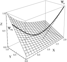
Figure 5.1. System state space (X,Y,Z) is shown. 2D slow manifold for the pure homogeneous system (6.3) is represented by a mesh. System stationary solution profile (6.6), black solid curve) in 1D case corresponds to 1D REDIM due to dimensional considerations. The approximation of the fast part of the homogeneous system (6.3) solution trajectory starting from the boundary state (6.8) is shown by the dashed line.

6. Analysis of 3D Michaelis-Menten model with the Laplacian Operator

The 3D Michaelis-Menten model is considered here as illustrative example of the REDIM approach. The original mathematical model of the enzyme biochemical system consists of three ODEs

(6.1) $$\frac{dX}{dt}=-XZ+L_{1}(1-Z-\mu(1-Y))$$

(6.2) $$\frac{dY}{dt}=-L_{3}YZ+\frac{L_{4}}{L_{2}}(1-Y)$$

(6.3) $$\frac{dZ}{dt}=\frac{1}{L_{2}}((-XZ+1-Z-\mu(1-Y))+\mu)-L_{3}YZ+\frac{L_{4}}{L_{2}}(1-Y)))$$

The system parameters are taken as $L_{1}=0.99$, $L_{2}=1$, $L_{3}=0.05$, $L_{4}=0.1$, $\mu=1$ (see e.g. [1, 19] for details and references). By taking the 1D diffusion into account we obtain the following PDEs system with the constant diffusion coefficient was taken as $\delta=0.01$:

(6.4) $$\frac{\partial X}{\partial t}=-XZ+L_{1}(1-Z-\mu(1-Y))+\delta\Delta X$$

(6.5) $$\frac{\partial Y}{\partial t}=-L_{3}YZ+\frac{L_{4}}{L_{2}}(1-Y)+\delta\Delta Y$$

(6.6) $$\frac{\partial Z}{\partial t}=\frac{1}{L_{2}}((-XZ+1-Z-\mu(1-Y))+\mu)-L_{3}YZ+\frac{L_{4}}{L_{2}}(1-Y)))+\delta\Delta Z$$

The system (6.6) is considered with the following initial and boundary conditions:

(6.7) $$\begin{pmatrix}X(t,0)=X_{eq}\\ Y(t,0)=Y_{eq}\\ Z(t,0)=Z_{eq}\\ \end{pmatrix}$$

(6.8) $$\begin{pmatrix}X(t,1)=2\\ Y(t,1)=0\\ Z(t,1)=1\\ \end{pmatrix}$$

(6.9) $$\begin{pmatrix}X(0,x)=(2-X_{eq})x+X_{eq}\\ Y(0,x)=(-Y_{eq})x+Y_{eq}\\ Z(0,x)=(1-Z_{eq})x+Z_{eq}\\ \end{pmatrix}$$

Here $(X_{eq},Y_{eq},Z_{eq})$ are coordinates of the equilibrium point and $x$ is spatial variable. Initial conditions are chosen to be a straight lines, they satisfy the general assumption - join initial and equilibrium values on the boundaries.

First, several numerical experiments were performed (see Fig. 5.1). A 2D slow manifold for homogeneous system (6.3) was found by Global Quasi-Linearisation (GQL) method [5] (see Appendix for a short description of GQL). Stationary system (6.6) solution profile was also integrated. Figure 5.1 shows a connection between the zero approximation of the slow manifold and the profile of the stationary system solution of the PDE in the original coordinates $(X,Y,Z)$. In Fig. 5.1 the system solution profile can be roughly subdivided into two parts: the slow part of the stationary solution that is very close to the slow manifold of the homogeneous system and second one, which is influenced by the diffusion term. The dashed line in this figure represents an approximation of linear fast sub-field (1D in this case).

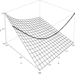
Figure 6.1. REDIM manifold (dashed line), exact stationary solution of the original PDE system (think line).

As in the previous section the main assumption remains the transport term is slow compared with the fast vector field. By applying the REDIM approach the stationary solution of the following system should represent the one-dimensional REDIM.

(6.10) $$\frac{\partial\Psi}{\partial t}=(I-\Psi_{\theta}\Psi_{\theta}^{+})(F_{R}+F_{D})$$

where following notations have been used, $I$ is 3x3 identity matrix, the system state vector

$$\Psi=\begin{pmatrix}X\\ Y\\ Z\end{pmatrix},$$

and projection matrix to the manifolds’ tangent space is given by

$$\Psi_{\theta}\Psi_{\theta}^{+}=\frac{1}{X_{\theta}^{2}+Y_{\theta}^{2}+Z_{\theta}^{2}}\begin{pmatrix}X_{\theta}^{2}&X_{\theta}Y_{\theta}&X_{\theta}Z_{\theta}\\ Y_{\theta}X_{\theta}&Y_{\theta}^{2}&Y_{\theta}Z_{\theta}\\ Z_{\theta}X_{\theta}&Z_{\theta}Y_{\theta}&Z_{\theta}^{2}\end{pmatrix},$$

and vector fields of reaction and diffusion terms

$$L\left(\Psi(\theta)\right)=\delta\theta_{x}^{2}\begin{pmatrix}X_{\theta\theta}\\ Y_{\theta\theta}\\ Z_{\theta\theta}\end{pmatrix},$$

$$\Phi\left(\Psi(\theta)\right)=\begin{pmatrix}-XZ+L_{1}(1-Z-\mu(1-Y))\\ -L_{3}YZ+\frac{L_{4}}{L_{2}}(1-Y)\\ \frac{1}{L_{2}}((-XZ+1-Z-\mu(1-Y))+\mu)-L_{3}YZ+\frac{L_{4}}{L_{2}}(1-Y)))\end{pmatrix}.$$

Here $\theta$ is the manifold parameter and $\theta_{x}$ is the gradient of the manifold parameter in $L\left(\Psi(\theta)\right)$. Now by using $\theta=X$ as a local manifold parameter, the system (6.10) can be simplified to only two equations for $Y=Y(\theta)$ and for $Z=Z(\theta)$. They were integrated and the stationary solution has been found for 1D REDIM, which is completely coincides with the system stationary profile (see Fig. 6.1).

The stationary solution of the system (6.10) whith $\theta=(\theta_{1},\theta_{2})$ represent 2D REDIM. Here $(\theta_{1}$,$\theta_{2})$ are two manifold parameters. In this case projection matrix of the manifold tangent space is considered by $\Psi_{\theta}\Psi_{\theta}^{+}$ where

$$\Psi_{\theta}=\begin{pmatrix}X_{\theta_{1}}&X_{\theta_{2}}\\ Y_{\theta_{1}}&Y_{\theta_{2}}\\ Z_{\theta_{1}}&Z_{\theta_{2}}\end{pmatrix},$$

and $\Psi_{\theta}^{+}$ is the Moore-Penrose pseudo-inverse of $\Psi_{\theta}$: $\Psi_{\theta}^{+}=(\Psi_{\theta}^{T}\Psi_{\theta})^{-1}\Psi_{\theta}^{T}$.

The components of the diffusion term $L\left(\Psi(\theta)\right)$ are the following:

$$L\left(\Psi(\theta)\right)^{X}=\delta(\theta_{1x},\theta_{2x})\begin{pmatrix}X_{\theta_{1}\theta_{1}}&X_{\theta_{1}\theta_{2}}\\ X_{\theta_{2}\theta_{1}}&X_{\theta_{2}\theta_{2}}\\ \end{pmatrix}\begin{pmatrix}\theta_{1x}\\ \theta_{2x}\\ \end{pmatrix},$$

$$L\left(\Psi(\theta)\right)^{Y}=\delta(\theta_{1x},\theta_{2x})\begin{pmatrix}Y_{\theta_{1}\theta_{1}}&Y_{\theta_{1}\theta_{2}}\\ Y_{\theta_{2}\theta_{1}}&Y_{\theta_{2}\theta_{2}}\\ \end{pmatrix}\begin{pmatrix}\theta_{1x}\\ \theta_{2x}\\ \end{pmatrix},$$

$$L\left(\Psi(\theta)\right)^{Z}=\delta(\theta_{1x},\theta_{2x})\begin{pmatrix}Z_{\theta_{1}\theta_{1}}&Z_{\theta_{1}\theta_{2}}\\ Z_{\theta_{2}\theta_{1}}&Z_{\theta_{2}\theta_{2}}\\ \end{pmatrix}\begin{pmatrix}\theta_{1x}\\ \theta_{2x}\\ \end{pmatrix}.$$

By using $\theta_{1}=X$, $\theta_{2}=Y$ as a local coordinates on the manifold of the system (6.10) can be simplified to only one equation for $Z=Z(\theta_{1},\theta_{2})$. It was integrated and the stationary solution has been found for 2D REDIM. Figure 6.2 shows a connection between the 2D REDIM, initial solution for the REDIM and/or slow homogeneous system manifold as in Figs.5.1 and 6.1. The stationary solution profile of the system illustrates the implementation and quality of the the REDIM approach to approximate the low- dimensional invariant manifold of relatively slow evolution of the reacting-diffusion system.

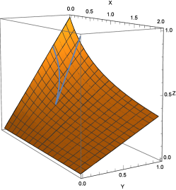
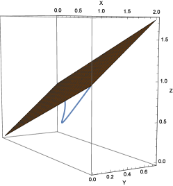
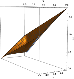
Figure 6.2. On the left: 2D slow homogeneous system manifold, in the middle: an initial solution for the REDIM and 2D REDIM manifold (shown on the right), exact stationary solution of the original PDE system (shown by thick line).

Figure 6.2 shows the stages of the REDIM construction. On the left the zero order approximation for a homogeneous system Eq. (6.3). In the middle one can see the stationary solution profile of the PDEs system Eq. (6.6), and on the right the converged stationary REDIM equation Eq. (6.10) solution is shown together with the stationary systems solution profile. One can see that 2D REDIM manifold approximates the relatively slow 2D system profile evolution. It means that when the system solution profile evolves Eq. (6.10) far form this surface it will evolve relatively fast (see subsection 4.1) towards 2D REDIM along the fast direction of the fast subspace (see Fig. 5.1) and then finally attains the stationary system solution profile. In this way, relative fast system dynamics cab be decoupled and the model is reduced to 2D model as a profile evolving within 2D REDIM.

7. Appendix(GQL and system decomposition)

Fast sub-fields and fast manifolds play a pivotal role in the theory and applications of the SPVF. The fast manifolds’ approximation is crucial for practical realization of the suggested SPVFs framework. A procedure for evaluation of the dimension and structure of fast sub-fields is proposed in this section.

In the case when fast manifolds and the system decomposition have linear structure they can be identified by a gap between the eigenvalues of an appropriate global linear approximation of the Right Hand Side (RHS) - vector function of a homogeneous system $\frac{d\psi}{dt}=F(\psi)$ (see [4] for detailed discussion)

$$T\psi\approx F\left(\psi\right).$$

Note that we did not use a hidden small parameter $\delta$ in $F\left(\psi\right)$, because its existence is not known ’a priori’ and has to be validated in a course of application of the GQL. Now, if $T$ has two groups of eigenvalues: so-called small eigenvalues $\lambda\left(\Lambda_{s}\right)$ and large eigenvalues $\lambda\left(\Lambda_{f}\right)$ that have sufficiently different order of magnitude, then the vector field $F(\psi)$ is regarded as linearly decomposed asymptotic singularly perturbed vector field [5]. Accordingly, fast and slow invariant sub-spaces given by columns of the matrices $Z_{f},\>Z_{s}$ corresponding [17] define the slow and variables . Namely,

(7.1) $$T\equiv\begin{pmatrix}Z_{f}&Z_{s}\end{pmatrix}\cdot\begin{pmatrix}\Lambda_{f}&0\\ 0&\Lambda_{s}\end{pmatrix}\cdot\begin{pmatrix}\tilde{Z_{f}}\\ \tilde{Z_{s}}\end{pmatrix},$$

now, if we denote

$$\tilde{Z}=Z^{-1}=\begin{pmatrix}Z_{f}&Z_{s}\end{pmatrix}^{-1}=\begin{pmatrix}\tilde{\left(Z_{f}\right)}_{m_{s}\times n}\\ \left(\tilde{Z_{s}}\right)_{m_{f}\times n}\end{pmatrix},$$

then, new coordinates suitable for an explicit decomposition (and coordinates transformation) are given by $(U,\,V)$:

(7.2) $$\begin{array}[]{c}U:=\tilde{Z}_{f}\,\psi\\ V:=\tilde{Z}_{s}\,\psi\end{array}.$$

The decomposed form and corresponding fast and slow subsystems becomes

(7.3) $$\left\{\begin{array}[]{c}\frac{dU}{dt}=\tilde{Z}_{f}\cdot F\left(\left(Z_{f}\>Z_{s}\right)\left(\begin{array}[]{c}U\\ V\end{array}\right)\right)\\ \frac{dV}{dt}=\tilde{Z}_{s}\cdot F\left(\left(Z_{f}\>Z_{s}\right)\left(\begin{array}[]{c}U\\ V\end{array}\right)\right)\end{array}\right..$$

The small system parameter controlling the characteristic time scales in (7.3) can be estimated by the gap between the smallest eigenvalue of the slow group and the largest eigenvalue of the fast group of eigenvalues [3]

(7.4) $$\varepsilon=\frac{max\left|\lambda\left(\Lambda_{s}\right)\right|}{min\left|\lambda\left(\Lambda_{f}\right)\right|}\ll 1.$$

In principle, the idea of the linear transformation is not new, see e.g. [21], but the principal point of the developed algorithm concerns evaluation of this transformation. We have developed the efficient and robust method that produces the best possible (to the leading order) decomposition with respect to existing multiple-scales hierarchy (see the attachment and [6, 7, 3] for more details).

8. Conclusions

The framework for manifolds based model reduction of the reaction-diffusion system has been established in the current work. This follows the original ideas of the singularly perturbed vector fields developed earlier. Within the suggested concept the problem of model reduction is treated as restriction of the original system to a low-dimensional manifold embedded in the systems state space. The manifold encounters the stationary states of the degenerate fast sub-field of the vector field defined by the reaction-diffusion system.

The main assumption of weak dependence of the fast system sub-filed of the reaction-diffusion PDEs vector field on the diffusion has been formulated. Under this assumption the theory of singularly perturbed vector fields was extended to the the systems with the molecular diffusion included. The developed framework can be used to justify the so-called REDIM method developed for reacting flow systems. For illustration Michaelis-Menten chemical kinetics model is extended to describe reaction-diffusion process. This example is used as an application that illustrate the method and the suggested framework. It was found that relatively fast 1D sub-field can be decoupled and the system can be reduced and represented by 2D reduced system.

References

- [1] Bykov V., Cherkinsky, Y., Mordeev, N., Gol’dshtein, V., Maas, U., Singularly Perturbed Profiles, submitted, 2016; Preprint: https://arxiv.org/pdf/1607.00486.pdf
- [2] Bykov, V., Maas, U., 2007, The Extension of the ILDM Concept to Reaction-Diffusion Manifolds, Combustion Theory and Modelling (CTM), 11 (6), 839-862.
- [3] Bykov, V., Maas, U., 2009, Problem Adapted Reduced Models Based on Reaction-Diffusion Manifolds (ReDiMs), Proc. Comb. Inst., 32(1): 561-568.
- [4] V. Bykov and U. Maas, Z. Phys. Chem., 223(4-5) (2009) 461–479.
- [5] Bykov, V., Goldfarb, I., Gol’dshtein, V., 2006, Singularly Perturbed Vector Fields, Journal of Physics: Conference Series, 55, 28-44.
- [6] Bykov. V., Gol’dshtein, V., Fast and Slow Invariant Manifolds for Chemical Kinetics, Computers & Mathematics with Applications, 65(10) (2013) 1502–1515.
- [7] Bykov, V., Gol’dshtein, V., Maas, U., 2008, Simple Global Reduction Technique Based on Decomposition Approach, Combustion Theory and Modelling (CTM), 12 (2), 389-405.
- [8] Bykov, V., Maas, U., 2009, Investigation of the Hierarchical Structure of Kinetic Models in Ignition Problems, Z. Phys. Chem., 223 (4-5), 461-479.
- [9] N. Fenichel, Geometric singular perturbation theory for ordinary differential equations, J Differential Equations, 31, 53-98 (1979).
- [10] V. Gol’dshtein, V. Sobolev, Integral manifolds in chemical kinetics and combustion, In Singularity theory and some problems of functional analysis, American Mathematical Society, 73-92 (1992).
- [11] I.Goldfarb, V.Gol’dshtein, U.Maas, Comparative Analysis of Two Assymptotic Approaches Based on Integral Manifolds, IMA J. of Applied Mathematics, 69, 353-374 (2004).
- [12] A.Gorban, I.Karlin, Methods of invarinat manifoldsfor kinetic problems, Journal of Chemical kinetics, 396, 197-403 (2002).
- [13] A.Gorban, I.Karlin, A.Zinoviev, Constructive methods of invariant manifolds for kinetic problems, Physics Reports, 396, 197-403 (2004).
- [14] H. G. Kaper, T.J. Kaper, Asymptotic Analysis of Two Reduction Methods for Systems of Chemical Reactions, Argonne National Lab, preprint ANL/MCS-P912-1001 (2001).
- [15] S.H. Lam, D.M. Goussis, The GSP method for simplifying kinetics, International Journal of Chemical Kinetics, 26, 461-486 (1994).
- [16] Maas, U., Bykov, V., 2011, The Extension of the Reaction/Diffusion Manifold Concept to Systems with Detailed Transport Models, Proc. Comb. Inst., 33(1):1253-1259.
- [17] U. Maas, S.B. Pope, Simplifying Chemical Kinetics: Intrinsic Low-Dimensional Manifolds in Composition Space, Combustion and Flame, 117, 99-116 (1992).
- [18] Marc R. Roussel and Simon J. Fraser, Global analysis of enzyme inhibition kinetics. J. Phys. Chem. 97, 8316-8327; errata, ibid. 98, 5174, (1993).
- [19] Marc R. Roussel and Simon J. Fraser, Invariant manifold methods for metabolic model reduction. Chaos 11, 196-206 (2001).
- [20] Yu.A.Mitropolskiy, O.B.Lykova, Lectures on the methods of integral manifolds (Kiev: Institute of Mathematics Ukrainen Akademy of Science, in Russian) (1968).
- [21] M.S. Okino and M.L. Mavrovouniotis, Chem. Rev., 98(2) (1998) 391–408.
- [22] C. Rhodes, M. Morari, S. Wiggins, Identification of the Low Order Manifolds:Validating the Algorithm of Maas and Pope, Chaos, 9, 108-123 (1999).