Adaptive Geometric Multiscale Approximations for Intrinsically Low-dimensional Data

Abstract

We consider the problem of efficiently approximating and encoding high-dimensional data sampled from a probability distribution $\rho$ in $\mathbb{R}^{D}$, that is nearly supported on a $d$-dimensional set $\mathcal{M}$ - for example supported on a $d$-dimensional Riemannian manifold. Geometric Multi-Resolution Analysis (GMRA) provides a robust and computationally efficient procedure to construct low-dimensional geometric approximations of $\mathcal{M}$ at varying resolutions. We introduce a thresholding algorithm on the geometric wavelet coefficients, leading to what we call adaptive GMRA approximations. We show that these data-driven, empirical approximations perform well, when the threshold is chosen as a suitable universal function of the number of samples $n$, on a wide variety of measures $\rho$, that are allowed to exhibit different regularity at different scales and locations, thereby efficiently encoding data from more complex measures than those supported on manifolds. These approximations yield a data-driven dictionary, together with a fast transform mapping data to coefficients, and an inverse of such a map. The algorithms for both the dictionary construction and the transforms have complexity $Cn\log n$ with the constant linear in $D$ and exponential in $d$. Our work therefore establishes adaptive GMRA as a fast dictionary learning algorithm with approximation guarantees. We include several numerical experiments on both synthetic and real data, confirming our theoretical results and demonstrating the effectiveness of adaptive GMRA.

Keywords: Dictionary Learning, Multi-Resolution Analysis, Adaptive Approximation, Manifold Learning, Compression

1 Introduction

We model a data set as $n$ i.i.d. samples $\mathcal{X}_{n}:=\{x_{i}\}_{i=1}^{n}$ from a probability measure $\rho$ in $\mathbb{R}^{D}$. We make the assumption that $\rho$ is supported on or near a set $\mathcal{M}$ of dimension $d\ll D$, and consider the problem, given $\mathcal{X}_{n}$, of learning a data-dependent dictionary that efficiently encodes data sampled from $\rho$.

In order to circumvent the curse of dimensionality, a popular model for data is sparsity: we say that the data is $k$-sparse on a suitable dictionary (i.e. a collection of vectors) $\Phi=\{\varphi_{i}\}_{i=1}^{m}\subset\mathbb{R}^{D}$ if each data point $x\in\mathbb{R}^{d}$ may be expressed as a linear combination of at most $k$ elements of $\Phi$. Clearly the case of interest is $k\ll D$. These sparse representations have been used in a variety of statistical signal processing tasks, compressed sensing, learning (see e.g. Protter and Elad, 2007; Peyré, 2009; Lewicki et al., 1998; Kreutz-Delgado et al., 2003; Maurer and Pontil, 2010; Chen et al., 1998; Donoho, 2006; Aharon et al., 2005; Candes and Tao, 2007, among many others), and spurred much research about how to learn data-adaptive dictionaries (see Gribonval et al., 2013; Vainsencher et al., 2011; Maurer and Pontil, 2010, and references therein). The algorithms used in dictionary learning are often computationally demanding, being based on high-dimensional non-convex optimization (Mairal et al., 2010). These approaches have the strength of being very general, with minimal assumptions made on geometry of the dictionary or on the distribution from which the samples are generated. This “worst-case” approach incurs bounds dependent upon the ambient dimension $D$ in general (even in the standard case of data lying on one hyperplane).

In Maggioni et al. (2016) we proposed to attack the dictionary learning problem under geometric assumptions on the data, namely that the data lies close to a low-dimensional set $\mathcal{M}$. There are of course various possible geometric assumptions, the simplest one being that $\mathcal{M}$ is a single $d$-dimensional subspace. For this model Principal Component Analysis (PCA) (see Pearson, 1901; Hotelling, 1933, 1936) is an effective tool to estimate the underlying plane. More generally, one may assume that data lie on a union of several low-dimensional planes instead of a single one. The problem of estimating multiple planes, called subspace clustering, is more challenging (see Fischler and Bolles, 1981; Ho et al., 2003; Vidal et al., 2005; Yan and Pollefeys, 2006; Ma et al., 2007, 2008; Chen and Lerman, 2009; Elhamifar and Vidal, 2009; Zhang et al., 2010; Liu et al., 2010; Chen and Maggioni, 2011). This model was shown effective in various applications, including image processing (Fischler and Bolles, 1981), computer vision (Ho et al., 2003) and motion segmentation (Yan and Pollefeys, 2006).

A different type of geometric model gives rise to manifold learning, where $\mathcal{M}$ is assumed to be a $d$-dimensional manifold isometrically embedded in $\mathbb{R}^{D}$, see (Tenenbaum et al., 2000; Roweis and Saul, 2000; Belkin and Niyogi, 2003; Donoho and Grimes, 2003; Coifman et al., 2005a, b; Zhang and Zha, 2004) and many others. It is of interest to move beyond this model to even more general geometric models, for example where the regularity of the manifold is reduced, and data is not forced to lie exactly on a manifold, but only close to it.

Geometric Multi-Resolution Analysis (GMRA) was proposed in Allard et al. (2012), and its finite-sample performance was analyzed in Maggioni et al. (2016). In GMRA, geometric approximations of $\mathcal{M}$ are constructed with multiscale techniques that have their roots in geometric measure theory, harmonic analysis and approximation theory. GMRA performs a multiscale tree decomposition of data and build multiscale low-dimensional geometric approximations to $\mathcal{M}$. Given data, we run the cover tree algorithm (Beygelzimer et al., 2006) to obtain a multiscale tree in which every node is a subset of $\mathcal{M}$, called a dyadic cell, and all dyadic cells at a fixed scale form a partition of $\mathcal{M}$. After the tree is constructed, we perform PCA on the data in each cell to locally approximate $\mathcal{M}$ by the $d$-dimensional principal subspace so that every point in that cell is only encoded by the $d$ coefficients in principal directions. At a fixed scale $\mathcal{M}$ is approximated by a piecewise linear set. In Allard et al. (2012) the performance of GMRA for volume measures on a $\mathcal{C}^{s},s\in(1,2]$ Riemannian manifold was analyzed in the continuous case (no sampling), and the effectiveness of GMRA was demonstrated empirically on simulated and real-world data. In Maggioni et al. (2016), the approximation error of $\mathcal{M}$ was estimated in the non-asymptotic regime with $n$ i.i.d. samples from a measure $\rho$, satisfying certain technical assumptions, supported on a tube of a $\mathcal{C}^{2}$ manifold of dimension $d$ isometrically embedded in $\mathbb{R}^{D}$. The probability bounds in Maggioni et al. (2016) depend on $n$ and $d$, but not on $D$, successfully avoiding the curse of dimensionality caused by the ambient dimension. The assumption that $\rho$ is supported in a tube around a manifold can account for noise and does not force the data to lie exactly on a smooth low-dimensional manifold.

In Allard et al. (2012) and Maggioni et al. (2016), GMRA approximations are constructed on uniform partitions in which all the cells have similar diameters. However, when the regularity, such as smoothness or curvature, weighted by the $\rho$ measure, of $\mathcal{M}$ varies at different scales and locations, uniform partitions are not optimal. Inspired by the adaptive methods in classical multi-resolution analysis (see Donoho and Johnstone, 1994, 1995; Cohen et al., 2002; Binev et al., 2005, 2007, among many others), we propose an adaptive version of GMRA to construct low-dimensional geometric approximations of $\mathcal{M}$ on an adaptive partition and provide finite sample performance guarantee for a much larger class of geometric structures $\mathcal{M}$ in comparison with Maggioni et al. (2016).

Our main result (Theorem 8) in this paper may be summarized as follows: Let $\rho$ be a probability measure supported on or near a compact $d$-dimensional Riemannian manifold $\mathcal{M}\hookrightarrow\mathbb{R}^{D}$, with $d\geq 3$. Let $\rho$ admit a multiscale decomposition satisfying the technical assumptions A1-A5 in section 2.1 below. Given $n$ i.i.d. samples are taken from $\rho$, the intrinsic dimension $d$, and a parameter $\kappa$ large enough, adaptive GMRA outputs a dictionary $\widehat{\Phi}_{n}=\{\widehat{\phi}_{i}\}_{i\in\mathcal{J}_{n}}$, an encoding operator $\widehat{\mathcal{D}}_{n}:\mathbb{R}^{D}\rightarrow\mathbb{R}^{\mathcal{J}_{n}}$ and a decoding operator $\widehat{\mathcal{D}}_{n}^{-1}:\mathbb{R}^{\mathcal{J}_{n}}\rightarrow\mathbb{R}^{D}$. With high probability, for every $x\in\mathbb{R}^{D}$, $\|\widehat{\mathcal{D}}_{n}x\|_{0}\leq d+1$ (i.e. only $d+1$ entries are non-zero), and the Mean Squared Error (MSE) satisfies

$${\rm MSE}:=\mathbb{E}_{x\sim\rho}[\|x-\widehat{\mathcal{D}}_{n}^{-1}\widehat{\mathcal{D}}_{n}x\|^{2}]\lesssim\left(\frac{\log n}{n}\right)^{\frac{2s}{2s+d-2}}.$$

Here $s$ is a regularity parameter of $\rho$ as in definition 5, which allows us to consider $\mathcal{M}$’s and $\rho$’s with nonuniform regularity, varying at different locations and scales. Note that the algorithm does not need to know $s$, but it automatically adapts to obtain a rate that depends on $s$. We believe, but do not prove, that this rate is indeed optimal. As for computational complexity, constructing $\widehat{\Phi}_{n}$ takes $\mathcal{O}((C^{d}+d^{2})Dn\log n)$ and computing $\widehat{\mathcal{D}}_{n}x$ only takes $\mathcal{O}(d(D+d^{2})\log n)$, which means we have a fast transform mapping data to their sparse encoding on the dictionary.

In adaptive GMRA, the dictionary is composed of the low-dimensional planes on adaptive partitions and the encoding operator transforms a point to the local $d$ principal coefficients of the data in a piece of the partition. We state this results in terms of encoding and decoding to stress that learning the geometry in fact yields efficient representations of data, which may be used for performing signal processing tasks in a domain where the data admit a sparse representation, e.g. in compressive sensing or estimation problems (see Iwen and Maggioni, 2013; Chen et al., 2012; Eftekhari and Wakin, 2015). Adaptive GMRA is designed towards robustness, both in the sense of tolerance to noise and to model error (i.e. data not lying on a manifold). We assume $d$ is given throughout this paper. If not, we refer to Little et al. (2012, 2009a, 2009b) for the estimation of intrinsic dimensionality.

The paper is organized as follows. Our main results, including the construction of GMRA, adaptive GMRA and their finite sample analysis, are presented in Section 2. We show numerical experiments in Section 3. The detailed analysis of GMRA and adaptive GMRA is presented in Section 4. In Section 5, we discuss the computational complexity of adaptive GMRA and extend our work to adaptive orthogonal GMRA. Proofs are postponed till the appendix.

Notation. We will introduce some basic notation here. $f\lesssim g$ means that there exists a constant $C$ independent on any variable upon which $f$ and $g$ depend, such that $f\leq Cg$. Similarly for $\gtrsim$. $f\asymp g$ means that both $f\lesssim g$ and $f\gtrsim g$ hold. The cardinality of a set $A$ is denoted by $\#A$. For $x\in\mathbb{R}^{D}$, $\|x\|$ denotes the Euclidean norm and $B_{r}(x)$ denotes the Euclidean ball of radius $r$ centered at $x$. Given a subspace $V\in\mathbb{R}^{D}$, we denote its dimension by $\dim(V)$ and the orthogonal projection onto $V$ by ${\rm Proj}_{V}$. If $A$ is a linear operator on $\mathbb{R}^{D}$, $||A||$ is its operator norm. The identity operator is denoted by $\mathbb{I}$.

2 Main results

GMRA was proposed in Allard et al. (2012) to efficiently represent points on or near a low-dimensional manifold in high dimensions. We refer the reader to that paper for details of the construction, and we summarize here the main ideas in order to keep the presentation self-contained. The construction of GMRA involves the following steps:

1. construct a multiscale tree $\boldsymbol{\mathcal{T}}$ and the associated decomposition of $\mathcal{M}$ into nested cells $\{C_{j,k}\}_{k\in\mathcal{K}_{j},j\in\mathbb{Z}}$ where $j$ represents scale and $k$ location;

2. perform local PCA on each $C_{j,k}$: let the mean (“center”) be $c_{j,k}$ and the $d$-dim principal subspace $V_{j,k}$. Define $\mathcal{P}^{j,k}(x):=c^{j,k}+{\rm Proj}_{V^{j,k}}(x-c^{j,k})$.

3. construct a “difference” subspace $W_{j+1,k^{\prime}}$ capturing $\mathcal{P}^{j,k}(C_{j,k})-\mathcal{P}^{j+1,k^{\prime}}(C_{j+1,k^{\prime}})$, for each $C_{j+1,k^{\prime}}\subseteq C_{j,k}$ (these quantities are associated with the refinement criterion in adaptive GMRA).

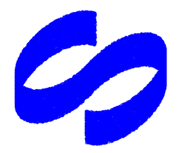
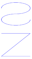
$\mathcal{M}$ may be approximated, at each scale $j$, by its projection $\mathcal{P}_{\Lambda_{j}}$ onto the family of linear sets $\Lambda_{j}:=\{\mathcal{P}_{j,k}(C_{j,k})\}_{k\in\mathcal{K}_{j}}$. For example, linear approximations of the S manifold at scale $6$ and $10$ are displayed in Figure 1. In a variety of distances, $\mathcal{P}_{\Lambda_{j}}(\mathcal{M})\rightarrow\mathcal{M}$.

(a) S manifold

(b) scale 6

(c) scale 10

Figure 1: (a) S manifold; (b,c) Linear approximations at scale $6,10$.

In practice $\mathcal{M}$ is unknown, and the construction above is carried over on training data, and its result is random with the training samples. Naturally we are interested in the performance of the construction on new samples. This is analyzed in a setting of “smooth manifold+noise” in Maggioni et al. (2016). When the regularity (such as smoothness or curvature) of $\mathcal{M}$ varies at different locations and scales, linear approximations on fixed uniform partitions are not optimal. Inspired by adaptive methods in classical multi-resolution analysis (see Cohen et al., 2002; Binev et al., 2005, 2007), we propose an adaptive version of GMRA which learns adaptive and near-optimal approximations.

We will start with the multiscale tree decomposition in Section 2.1 and present GMRA and adaptive GMRA in Section 2.3 and 2.4 respectively.

2.1 Multiscale partitions and trees

A multiscale set of partitions of $\mathcal{M}$ with respect to probability measure $\rho$ is a family of sets $\{C_{j,k}\}_{k\in\mathcal{K}_{j},j\in\mathbb{Z}}$, called dyadic cells, satisfying Assumptions (A1-A5) below for all integers $j\geq j_{\rm min}$:

(A1)

for any $k\in\mathcal{K}_{j}$ and $k^{\prime}\in\mathcal{K}_{j+1}$, either $C_{j+1,k^{\prime}}\subseteq C_{j,k}$ or $\rho(C_{j+1,k^{\prime}}\cap C_{j,k})=0$. We denote the children of $C_{j,k}$ by ${\mathscr{C}}(C_{j,k})=\{C_{j+1,k^{\prime}}:C_{j+1,k^{\prime}}\subseteq C_{j,k}\}$. We assume that $a_{\rm min}\leq\#{\mathscr{C}}(C_{j,k})\leq a_{\rm max}$. Also for every $C_{j,k}$, there exists a unique $k^{\prime}\in\mathcal{K}_{j-1}$ such that $C_{j,k}\subseteq C_{j-1,k^{\prime}}$. We call $C_{j-1,k^{\prime}}$ the parent of $C_{j,k}$.

(A2)

$\rho(\mathcal{M}\setminus\cup_{k\in\mathcal{K}_{j}}C_{j,k})=0$, i.e. $\Lambda_{j}:=\{C_{j,k}\}_{k\in\mathcal{K}_{j}}$ is a cover for $\mathcal{M}$.

(A3)

$\exists\theta_{1}>0\,:\,\#\Lambda_{j}\leq 2^{jd}/\theta_{1}$.

(A4)

$\exists\theta_{2}>0$ such that, if $x$ is drawn from $\rho|_{C_{j,k}}$, then a.s. $\|x-c_{j,k}\|\leq\theta_{2}2^{-j}.$

(A5)

Let $\lambda_{1}^{j,k}\geq\lambda_{2}^{j,k}\geq\ldots\geq\lambda_{D}^{j,k}$ be the eigenvalues of the covariance matrix $\Sigma_{j,k}$ of $\rho|_{C_{j,k}}$, defined in Table 1. Then:

• $\exists\theta_{3}>0$ such that $\forall j\geq j_{\rm min}$ and $k\in\mathcal{K}_{j}$, $\lambda_{d}^{j,k}\geq\theta_{3}{2^{-2j}}/{d}$,

• $\exists\theta_{4}\in(0,1)$ such that $\lambda_{d+1}^{j,k}\leq\theta_{4}\lambda_{d}^{j,k}$.

(A1) implies that the $\{C_{j,k}\}_{k\in\mathcal{K}_{j},j\geq j_{\rm min}}$ are associated with a tree structure, and with some abuse of notation we call the above tree decompositions. (A1)-(A5) are natural assumptions, easily satisfied by natural multiscale decompositions when $\mathcal{M}$ is a $d$-dimensional manifold isometrically embedded in $\mathbb{R}^{D}$: see the work (Maggioni et al., 2016) for a detailed discussion. (A2) guarantees that the cells at scale $j$ form a partition of $\mathcal{M}$; (A3) says that there are at most $2^{jd}/\theta_{1}$ dyadic cells at scale $j$. (A4) ensures ${\rm diam}(C_{j,k})\lesssim 2^{-j}$. When $\mathcal{M}$ is a $d$-dimensional manifold, (A5)(i) is the condition that the best rank $d$ approximation to $\Sigma_{j,k}$ is close to the covariance matrix of a $d$-dimensional Euclidean ball, while (A5)(ii) imposes that the $(d+1)$-th eigenvalue is smaller that the $d$-th eigenvalue, i.e. the set has significantly larger variances in $d$ directions than in all the remaining ones.

We will construct such $\{C_{j,k}\}_{k\in\mathcal{K}_{j},j\geq j_{\rm min}}$ in Section 2.6. In our construction (A1-A4) is satisfied when $\rho$ a doubling probability measure (see Christ, 1990; Deng and Han, 2008). If we further assume that $\mathcal{M}$ is a $d$-dimensional $\mathcal{C}^{s},s\in(1,2]$ closed Riemannian manifold isometrically embedded in $\mathbb{R}^{D}$, then (A5) is satisfied as well (See Proposition 13).

Some notation: a master tree $\mathcal{T}$ is associated with $\{C_{j,k}\}_{k\in\mathcal{K}_{j},j\geq j_{\rm min}}$ (using property (A1)), constructed on $\mathcal{M}$; since $C_{j,k}$’s at scale $j$ have similar diameters, $\Lambda_{j}:=\{C_{j,k}\}_{k\in\mathcal{K}_{j}}$ is called a uniform partition at scale $j$. It may happen that at the coarsest scales conditions (A3)-(A5) are satisfied but with very poor constants $\bf\theta$: it will be clear that in all that follows we may discard a few coarse scales, and only work at scales that are fine enough and for which (A3)-(A5) truly capture the local geometry of $\mathcal{M}$.

A proper subtree $\tilde{\mathcal{T}}$ of $\mathcal{T}$ is a collection of nodes of $\mathcal{T}$ with the properties: (i) the root node is in $\tilde{\mathcal{T}}$, (ii) if $C_{j,k}$ is in $\tilde{\mathcal{T}}$ then the parent of $C_{j,k}$ is also in $\tilde{\mathcal{T}}$. Any finite proper subtree $\tilde{\mathcal{T}}$ is associated with a unique partition $\Lambda=\Lambda(\tilde{\mathcal{T}})$ which consists of its outer leaves, by which we mean those $C_{j,k}\in\mathcal{T}$ such that $C_{j,k}\notin\tilde{\mathcal{T}}$ but its parent is in $\tilde{\mathcal{T}}$.

	GMRA	Empirical GMRA
Linear projection on $C_{j,k}$	$\mathcal{P}_{j,k}(x):=c_{j,k}+{\rm Proj}_{V_{j,k}}(x-c_{j,k})$	$\widehat{\mathcal{P}}_{j,k}(x):=\widehat{c}_{j,k}+{\rm Proj}_{\widehat{V}_{j,k}}(x-\widehat{c}_{j,k})$
Linear projection at scale $j$	$\mathcal{P}_{j}:=\sum_{k\in\mathcal{K}_{j}}\mathcal{P}_{j,k}\mathbf{1}_{{j,k}}$	$\widehat{\mathcal{P}}_{j}:=\sum_{k\in\mathcal{K}_{j}}\widehat{\mathcal{P}}_{j,k}\mathbf{1}_{{j,k}}$
Measure	$\rho(C_{j,k})$	$\widehat{\rho}(C_{j,k})=\widehat{n}_{j,k}/n$
Center	$c_{j,k}:=\mathbb{E}_{j,k}x$	$\widehat{c}_{j,k}:=\frac{1}{\widehat{n}_{j,k}}\textstyle\sum_{x_{i}\in C_{j,k}}x_{i}$
Principal subspaces	$V_{j,k}$ minimizes $\mathbb{E}_{j,k}\|x-c_{j,k}-{\rm Proj}_{V}(x-c_{j,k})\|^{2}$ among $d$-dim subspaces	$\widehat{V}_{j,k}$ minimizes $\frac{1}{\widehat{n}_{j,k}}\textstyle\sum_{x_{i}\in C_{j,k}}\|x-\widehat{c}_{j,k}-{\rm Proj}_{V}(x-\widehat{c}_{j,k})\|^{2}$ among $d$-dim subspaces
Covariance matrix	$\Sigma_{j,k}:=\mathbb{E}_{j,k}(x-c_{j,k})(x-c_{j,k})^{T}$	$\widehat{\Sigma}_{j,k}:=\frac{1}{\widehat{n}_{j,k}}\sum_{x_{i}\in C_{j,k}}(x_{i}-\widehat{c}_{j,k})(x_{i}-\widehat{c}_{j,k})^{T}$
$\langle\mathcal{P}X,\mathcal{Q}X\rangle$	$\int_{\mathcal{M}}\langle\mathcal{P}x,\mathcal{Q}x\rangle d\rho$	${1}/{n}\sum_{x_{i}\in\mathcal{X}_{n}}\langle\mathcal{P}x_{i},\mathcal{Q}x_{i}\rangle$
$\|\mathcal{P}X\|$	$\left(\int_{\mathcal{M}}\|\mathcal{P}x\|^{2}d\rho\right)^{\frac{1}{2}}$	$\left({1}/{n}\sum_{x_{i}\in\mathcal{X}_{n}}\|\mathcal{P}x_{i}\|^{2}\right)^{\frac{1}{2}}$

Table 1: $\mathbf{1}_{j,k}$ is the indicator function on $C_{j,k}$ (i.e.,$\mathbf{1}_{j,k}(x)=1$ if $x\in C_{j,k}$ and $0$ otherwise). Here $\mathbb{E}_{j,k}$ stands for expectation with respect to the conditional distribution $d\rho|_{C_{j,k}}$. The measure of $C_{j,k}$ is $\rho(C_{j,k})$ and the empirical measure is $\widehat{\rho}(C_{j,k})=\widehat{n}_{j,k}/n$ where $\widehat{n}_{j,k}$ is the number of points in $C_{j,k}$. $V_{j,k}$ and $\widehat{V}_{j,k}$ are the eigen-spaces associated with the largest $d$ eigenvalues of $\Sigma_{j,k}$ and $\widehat{\Sigma}_{j,k}$ respectively. Here $\mathcal{P},\mathcal{Q}$: $\mathcal{M}\to\mathbb{R}^{D}$ are two operators.

2.2 Empirical GMRA

In practice the master tree $\mathcal{T}$ is not given, nor can be constructed since $\mathcal{M}$ is not known: we will construct one on samples by running a variation of the cover tree algorithm (see Beygelzimer et al., 2006). From now on we denote the training data by $\mathcal{X}_{2n}$. We randomly split the data into two disjoint groups such that $\mathcal{X}_{2n}=\mathcal{X}^{\prime}_{n}\cup\mathcal{X}_{n}$ where $\mathcal{X}^{\prime}_{n}=\{x^{\prime}_{1},\ldots,x^{\prime}_{n}\}$ and $\mathcal{X}_{n}=\{x_{1},\ldots,x_{n}\}$, apply the cover tree algorithm (see Beygelzimer et al., 2006) on $\mathcal{X}_{n}^{\prime}$ to construct a tree satisfying (A1-A5) (see section 2.6). After the tree is constructed, we assign points in the second half of data $\mathcal{X}_{n}$, to the appropriate cells. In this way we obtain a family of multiscale partitions for the points in $\mathcal{X}_{n}$, which we truncate to the largest subtree whose leaves contain at least $d$ points in $\mathcal{X}_{n}$. This subtree is called the data master tree, denoted by $\mathcal{T}^{n}$. We then use $\mathcal{X}_{n}$ to perform local PCA to obtain the empirical mean $\widehat{c}_{j,k}$ and the empirical $d$-dimensional principal subspace $\widehat{V}_{j,k}$ on each $C_{j,k}$. Define the empirical projection $\widehat{\mathcal{P}}_{j,k}(x):=\widehat{c}_{j,k}+{\rm Proj}_{\widehat{V}_{j,k}}(x-\widehat{c}_{j,k})$ for $x\in C_{j,k}$. Table 1 summarizes the GMRA objects and their empirical counterparts.

2.3 Geometric Multi-Resolution Analysis: uniform partitions

GMRA with respect to the distribution $\rho$ associated with the multiscale tree $\mathcal{T}$ consists a collection of piecewise affine projectors $\{\mathcal{P}_{j}:\mathbb{R}^{D}\rightarrow\mathbb{R}^{D}\}_{j\geq j_{\rm min}}$ on the multiscale partitions $\{\Lambda_{j}:=\{C_{j,k}\}_{k\in\mathcal{K}_{j}}\}_{j\geq j_{\rm min}}$. At scale $j$, $\mathcal{M}$ is approximated by the piecewise linear sets $\{\mathcal{P}_{j,k}(C_{j,k})\}_{k\in\mathcal{K}_{j}}$. In order to understand the empirical approximation error of $\mathcal{M}$ by the piecewise linear sets $\{\widehat{\mathcal{P}}_{j,k}(C_{j,k})\}_{k\in\mathcal{K}_{j}}$ at scale $j$, we split the error into a squared bias term and a variance term:

$$\mathbb{E}\|X-\widehat{\mathcal{P}}_{j}X\|^{2}=\underbrace{\|X-\mathcal{P}_{j}X\|^{2}}_{\text{bias}^{2}}+\underbrace{\mathbb{E}\|\mathcal{P}_{j}X-\widehat{\mathcal{P}}_{j}X\|^{2}}_{\text{variance}}.$$ (1)

$\mathbb{E}\|X-\widehat{\mathcal{P}}_{j}X\|^{2}$ is also called the Mean Square Error (MSE) of GMRA. To bound the bias term, we need regularity assumptions on the $\rho$, and for the variance term we prove concentration bounds of the relevant quantities around their expected values.

For a fixed distribution $\rho$, the approximation error of $\mathcal{M}$ at scale $j$, measured by $\|X-\mathcal{P}_{j}X\|:=\|(\mathbb{I}-\mathcal{P}_{j})X\|$, decays at a rate dependent on the regularity of $\mathcal{M}$ in the $\rho$-measure (see Allard et al., 2012). We quantify the regularity of $\rho$ as follows:

Definition 1 (Model class $\mathcal{A}_{s}$)

A probability measure $\rho$ supported on $\mathcal{M}$ is in $\mathcal{A}_{s}$ if

$$|\rho|_{\mathcal{A}_{s}}=\sup_{\mathcal{T}}\ \inf\{A_{0}\,:\,\|X-\mathcal{P}_{j}X\|\leq A_{0}2^{-js},\forall\,j\geq j_{\rm min}\}<\infty\,,$$ (2)

where $\mathcal{T}$ varies over the set, assumed non-empty, of multiscale tree decompositions satisfying Assumption (A1-A5).

We capture the case where the $L^{2}$ approximation error is roughly the same on every cell with the following definition:

Definition 2 (Model class $\mathcal{A}_{s}^{\infty}$)

A probability measure $\rho$ supported on $\mathcal{M}$ is in $\mathcal{A}_{s}^{\infty}$ if

$$|\rho|_{\mathcal{A}_{s}^{\infty}}=\sup_{\mathcal{T}}\ \inf\{A_{0}\,:\,\|(X-\mathcal{P}_{j,k}X)\mathbf{1}_{j,k}\|\leq A_{0}2^{-js}\sqrt{\rho(C_{j,k})},\ \forall\,k\in\mathcal{K}_{j},j\geq j_{\rm min}\}<\infty\$$ (3)

where $\mathcal{T}$ varies over the set, assumed non-empty, of multiscale tree decompositions satisfying Assumption (A1-A5).

Clearly $\mathcal{A}_{s}^{\infty}\subset\mathcal{A}_{s}$. Also, since ${\rm diam}(C_{j,k})\leq 2\theta_{2}2^{-j}$, necessarily $\|(\mathbb{I}-\mathcal{P}_{j,k})\mathbf{1}_{j,k}X\|\leq\theta_{2}2^{-j}\sqrt{\rho(C_{j,k})},\ \forall\,k\in\mathcal{K}_{j},j\geq j_{\rm min}$, and therefore $\rho\in\mathcal{A}_{1}^{\infty}$ in any case. Finally, these classes contain suitable measures supported on manifolds:

Proposition 3

Let $\mathcal{M}$ be a closed manifold of class $\mathcal{C}^{s}$, $s\in(1,2]$ isometrically embedded in $\mathbb{R}^{D}$, and $\rho$ be a doubing probability measure on $\mathcal{M}$ with the doubling constant $C_{1}$. Then our construction of $\{C_{j,k}\}_{k\in\mathcal{K}_{j},j\geq j_{\rm min}}$ in Section 2.6 satisfies (A1-A5), and $\rho\in\mathcal{A}_{s}^{\infty}$.

Proposition 3 is proved in Appendix A.2.

Example 1

We consider the $d$-dim S manifold whose $x_{1}$ and $x_{2}$ coordinates are on the $S$ curve and $x_{i}\in[0,1],i=3,\ldots,d+1$. As stated above, the volume measure on the S manifold is in $\mathcal{A}_{2}^{\infty}$. Numerically one can identify $s$ from data sampled from $\rho\in\mathcal{A}_{s}$ as the slope of the line approximating $\log_{10}\|X-\mathcal{P}_{j}X\|$ as a function of $\log_{10}r_{j}$ where $r_{j}$ is the average diameter of $C_{j,k}$’s at scale $j$. Our numerical experiments in Figure 5 (b) give rise to $s\approx 2.0239,2.1372,2.173$ when $d=3,4,5$ respectively.

Example 2

For comparison we consider the $d$-dimensional Z manifold whose $x_{1}$ and $x_{2}$ coordinates are on the $Z$ curve and $x_{i}\in[0,1],i=3,\ldots,d+1$. Volume measure on the Z manifold is in $\mathcal{A}_{1.5}$ (see appendix B.2). Our numerical experiments in Figure 5 (c) give rise to $s\approx 1.5367,1.6595,1.6204$ when $d=3,4,5$ respectively.

The squared bias in (1) satisfies $\|X-\mathcal{P}_{j}X\|^{2}\leq|\rho|_{\mathcal{A}_{s}}^{2}2^{-2js}$ whenever $\rho\in\mathcal{A}_{s}$. In Proposition 15 we will show that the variance term is estimated in terms of the sample size $n$ and the scale $j$:

$$\mathbb{E}\|\mathcal{P}_{j}X-\widehat{\mathcal{P}}_{j}X\|^{2}\leq\frac{d^{2}\#\Lambda_{j}\log[\alpha d\#\Lambda_{j}]}{\beta 2^{2j}n}{=\mathcal{O}\left(\frac{j2^{j(d-2)}}{n}\right),}$$

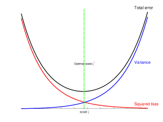
where $\alpha,\beta$ are constants depending on $\theta_{2},\theta_{3}$. In the case $d=1$ both the squared bias and the variance decrease as $j$ increases, so choosing the finest scale of the data tree $\mathcal{T}^{n}$ yields the best rate of convergence. When $d\geq 2$, the squared bias decreases but the variance increases as $j$ gets large as shown Figure 2, as a manifestation of the bias-variance tradeoff in classical statistical and machine learning, except that it arises here in a geometric setting. By choosing a proper scale $j$ to balance these two terms, we obtain the following rate of convergence for empirical GMRA:

(a) Bias and variance tradeoff

(b) Error versus the partition size

Figure 2: (a) Plot of the bias and variance estimates in Eq. (1), with $s=2,d=5,n=100$. (b) shows the approximation error on test data versus the partition size in GMRA and adaptive GMRA for the 3-dim S manifold. When the partition size is between $1$ and $10^{2.8}$, the bias dominates the error so the error decreases; after that, the variance dominates the error, which becomes increasing.

Theorem 4

Suppose $\rho\in\mathcal{A}_{s}$ for $s\geq 1$. Let $\nu>0$ be arbitrary and $\mu>0$. Let $j^{*}$ be chosen such that

$$2^{-j^{*}}=\begin{cases}\mu\frac{\log n}{n}&\text{ for }d=1\\ \mu\left(\frac{\log n}{n}\right)^{\frac{1}{2s+d-2}},&\text{ for }d\geq 2\end{cases}$$ (4)

then there exists $C_{1}:=C_{1}(\theta_{1},\theta_{2},\theta_{3},\theta_{4},d,\nu,\mu)$ and $C_{2}:=C_{2}(\theta_{1},\theta_{2},\theta_{3},\theta_{4},d,\mu)$ such that:

$$\mathbb{P}\left\{\|X-\widehat{\mathcal{P}}_{j^{*}}X\|\geq(|\rho|_{\mathcal{A}_{s}}\mu^{s}+C_{1})\frac{\log n}{n}\right\}\leq C_{2}n^{-\nu},\quad \text{for }d=1,$$ (5)

$$\mathbb{P}\left\{\|X-\widehat{\mathcal{P}}_{j^{*}}X\|\geq(|\rho|_{\mathcal{A}_{s}}\mu^{s}+C_{1})\left(\frac{\log n}{n}\right)^{\frac{s}{2s+d-2}}\right\}\leq C_{2}n^{-\nu},\quad \text{for }d\geq 2\,.$$ (6)

Theorem 4 is proved in Section 4.2. In the perspective of dictionary learning, GMRA provides a dictionary $\Phi_{j^{*}}$ of cardinality $\asymp dn/\log n$ for $d=1$ and of cardinality $\asymp d(n/\log n)^{\frac{d}{2s+d-2}}$ for $d\geq 2$, so that every $x$ sampled from $\rho$ (and not just samples in the training data) may be encoded with a vector with $d+1$ nonzero entries: one entry encodes the location $k$ of $x$ on the tree, e.g. $(j^{*},x)=(j^{*},k)$ such that $x\in C_{j^{*},k}$, and the other $d$ entries are $\widehat{V}_{j^{*},x}^{T}(x-\widehat{c}_{j^{*},x})$. We also remind the reader that GMRA automatically constructs a fast transform mapping points $x$ to the vector representing $\Phi_{j^{*}}$ (See Allard et al. (2012); Maggioni et al. (2016) for a discussion). Note that by choosing $\nu$ large enough,

$$\eqref{thm2eq1}\implies{\rm MSE}=\mathbb{E}\|X-\widehat{\mathcal{P}}_{j^{*}}X\|^{2}\lesssim\left(\frac{\log n}{n}\right)^{\frac{2s}{2s+d-2}}\,,$$

and (5) implies MSE $\lesssim(\frac{\log n}{n})^{2}$ for $d=1$. Clearly, one could fix a desired MSE of size $\varepsilon^{2}$, and obtain from the above a dictionary of size dependent only of $\varepsilon$ and independent of $n$, for $n$ sufficiently large, thereby obtaining a way of compressing data (see Maggioni et al. (2016) for further discussion on this point). A special case of Theorem 4 with $s=2$ was proved in Maggioni et al. (2016).

2.4 Geometric Multi-Resolution Analysis: Adaptive Partitions

	Definition (infinite sample)	Empirical version
Difference operator	$\mathcal{Q}_{j,k}:=(\mathcal{P}_{j}-\mathcal{P}_{j+1})\mathbf{1}_{j,k}$	$\widehat{\mathcal{Q}}_{j,k}:=(\widehat{\mathcal{P}}_{j}-\widehat{\mathcal{P}}_{j+1})\mathbf{1}_{j,k}$
Norm of difference	$\Delta_{j,k}^{2}:=\int_{C_{j,k}}\|\mathcal{Q}_{j,k}x\|^{2}d\rho$	$\widehat{\Delta}_{j,k}^{2}:=\frac{1}{n}\sum_{x_{i}\in C_{j,k}}\|\widehat{\mathcal{Q}}_{j,k}x_{i}\|^{2}$

Table 2: Refinement criterion and the empirical version

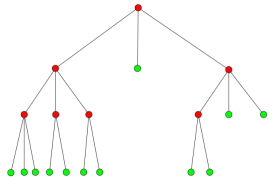
The performance guarantee in Theorem 4 is not fully satisfactory for two reasons: (i) the regularity parameter $s$ is required to be known to choose the optimal scale $j^{*}$, and this parameter is typically unknown in any practical setting, and (ii) none of the uniform partitions $\{C_{j,k}\}_{k\in\mathcal{K}_{j}}$ will be optimal if the regularity of $\rho$ (and/or $\mathcal{M}$) varies at different locations and scales. This lack of uniformity in regularity appears in a wide variety of data sets: when clusters exist that have cores denser than the remaining regions of space, when trajectories of a dynamical system are sampled that linger in certain regions of space for much longer time intervals than others (e.g. metastable states in molecular dynamics (Rohrdanz et al., 2011; Zheng et al., 2011)), in data sets of images where details exist at different level of resolutions, affecting regularity at different scales in the ambient space, and so on. To fix the ideas we consider again one simplest manifestations of this phenomenon in the examples considered above: uniform partitions work well for the volume measure on the S manifold but are not optimal for the volume measure on the Z manifold, for which the ideal partition is coarse on flat regions but finer at and near the corners (see Figure 4). In applications, for example to mesh approximation, it is often the case that the point clouds to be approximated are not uniformly smooth and include different levels of details at different locations and scales (see Figure 8). Thus we propose an adaptive version of GMRA that will automatically adapts to the regularity of the data and choose a near-optimal adaptive partition.

Figure 3: Left: a master tree in which red nodes satisfy $\Delta_{j,k}\geq 2^{-j}\tau_{n}$ but blue nodes do not. Right: the subtree of the red nodes is the smallest proper subtree that contains all the nodes satisfying $\Delta_{j,k}\geq 2^{-j}\tau_{n}$, i.e. were red in the figure on the left. Green nodes form the adaptive partition.

Algorithm 1 Empirical adaptive GMRA

0:  data $\mathcal{X}_{2n}=\mathcal{X}_{n}^{\prime}\cup\mathcal{X}_{n}$, intrinsic dimension $d$, threshold $\kappa$

0:  $\mathcal{T}^{n}$, $\{C_{j,k}\}$, $\widehat{\mathcal{P}}_{\widehat{\Lambda}_{\tau_{n}}}$ : multiscale tree, corresponding cells and adaptive piecewise linear projectors on adaptive partition.

1:  Construct $\mathcal{T}^{n}$ and $\{C_{j,k}\}$ from $\mathcal{X}^{\prime}_{n}$

2:  Now use $\mathcal{X}_{n}$. Compute $\widehat{\mathcal{P}}_{j,k}$ and $\widehat{\Delta}_{j,k}$ on every node $C_{j,k}\in\mathcal{T}^{n}$.

3:  $\widehat{\mathcal{T}}_{\tau_{n}}\leftarrow$ smallest proper subtree of $\mathcal{T}^{n}$ containing all $C_{j,k}\in\mathcal{T}^{n}$ : $\widehat{\Delta}_{j,k}\geq 2^{-j}\tau_{n}$ where $\tau_{n}=\kappa\sqrt{(\log n)/n}$.

4:  $\widehat{\Lambda}_{\tau_{n}}\leftarrow$ partition associated with outer leaves of $\widehat{\mathcal{T}}_{\tau_{n}}$

5:  $\widehat{\mathcal{P}}_{\widehat{\Lambda}_{\tau_{n}}}\leftarrow\sum_{C_{j,k}\in\widehat{\Lambda}_{\tau_{n}}}\widehat{\mathcal{P}}_{j,k}\mathbf{1}_{j,k}.$

Adaptive partitions may be effectively selected with a criterion that determines whether or not a cell should participate to the adaptive partition. The quantities involved in the selection and their empirical version are summarized in Table 2.

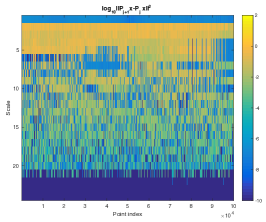
We expect $\Delta_{j,k}$ to be small on approximately flat regions, and large $\Delta_{j,k}$ at many scales at irregular locations. We also expect $\widehat{\Delta}_{j,k}$ to have the same behavior, at least when $\widehat{\Delta}_{j,k}$ is with high confidence close to $\Delta_{j,k}$. We see this phenomenon represented in Figure 4 (a,b): as $j$ increases, for the S manifold $\|\widehat{\mathcal{P}}_{j+1}x_{i}-\widehat{\mathcal{P}}_{j}x_{i}\|$ decays uniformly at all points, while for the Z manifold, the same quantity decays rapidly on flat regions but remains large at fine scales around the corners. We wish to include in our approximation the nodes where this quantity is large, since we may expect a large improvement in approximation by including such nodes. However if too few samples exist in a node, then this quantity is not to be trusted, because its variance is large. It turns out that it is enough to consider the following criterion: let $\widehat{\mathcal{T}}_{\tau_{n}}$ be the smallest proper subtree of $\mathcal{T}^{n}$ that contains all $C^{j,k}\in\mathcal{T}^{n}$ for which $\widehat{\Delta}_{j,k}\geq 2^{-j}\tau_{n}$ where $\tau_{n}=\kappa\sqrt{(\log n)/n}$. Crucially, $\kappa$ may be chosen independently of the regularity index (see Theorem 8). Empirical adaptive GMRA returns piecewise affine projectors on $\widehat{\Lambda}_{\tau_{n}}$, the partition associated with the outer leaves of $\widehat{\mathcal{T}}_{\tau_{n}}$. Our algorithm is summarized in Algorithm 1.

(a) S manifold

(b) Z manifold

(c) Error vs partition size, S manifold

(d) Adaptive approx. of S

(e) Adaptive approx. of Z

(f) Error vs partition size, Z manifold

Figure 4: (a,b): $\log_{10}||\widehat{\mathcal{P}}_{j}(x_{i})-\widehat{\mathcal{P}}_{j+1}(x_{i})||$ from the coarsest scale (top) to the finest scale (bottom), with columns indexed by points, sorted from left to right on the manifold. (d,e): adaptive approximations. (c,f): log-log plot of the approximation error versus the partition size in GMRA and adaptive GMRA respectively. Theoretically, the slope is $-2/d$ in both GMRA and adaptive GMRA for the S manifold. For the Z manifold, the slope is $-1.5/d$ in GMRA and $-{1.5/(d-1)}$ in adaptive GMRA (see appendix B).

We will provide a finite sample performance guarantee of the empirical adaptive GMRA for a model class that is more general than $\mathcal{A}_{s}^{\infty}$. Given any fixed threshold $\eta>0$, we let $\mathcal{T}_{(\rho,\eta)}$ be the smallest proper tree of $\mathcal{T}$ that contains all $C_{j,k}\in\mathcal{T}$ for which $\Delta_{j,k}\geq 2^{-j}\eta$. The corresponding adaptive partition $\Lambda_{(\rho,\eta)}$ consists of the outer leaves of $\mathcal{T}_{(\rho,\eta)}$. We let $\#_{j}\mathcal{T}_{(\rho,\eta)}$ be the number of cells in $\mathcal{T}_{(\rho,\eta)}$ at scale $j$.

Definition 5 (Model class $\mathcal{B}_{s}$)

In the case $d\geq 3$, given $s>0$, a probability measure $\rho$ supported on $\mathcal{M}$ is in $\mathcal{B}_{s}$ if $\rho$ satisfies the following regularity condition:

$$|\rho|_{\mathcal{B}_{s}}^{p}:=\sup_{{\mathcal{T}}}\ \sup_{\eta>0}\eta^{p}\sum_{j\geq j_{\rm min}}2^{-2j}\#_{j}\mathcal{T}_{(\rho,\eta)}<\infty,\,\,\text{ with }p=\frac{2(d-2)}{2s+d-2}$$ (7)

where $\mathcal{T}$ varies over the set, assumed nonempty, of multiscale tree decompositions satisfying Assumption (A1-A5).

For elements in the model class $\mathcal{B}_{s}$ we have control on the growth rate of the truncated tree $\mathcal{T}_{(\rho,\eta)}$ as $\eta$ decreases, namely it is $\mathcal{O}(\eta^{-p})$. The key estimate on variance and sample complexity in Lemma 14 indicates that the natural measure of the complexity of $\mathcal{T}_{(\rho,\eta)}$ is the weighted tree complexity measure $\sum_{j\geq j_{\rm min}}2^{-2j}\#_{j}\mathcal{T}_{(\rho,\eta)}$ in the definition above. First of all, the class $\mathcal{B}_{s}$ is indeed larger than $\mathcal{A}_{s}^{\infty}$ (see appendix A.4 for a proof):

Lemma 6

$\mathcal{B}_{s}$ is a more general model class than $\mathcal{A}_{s}^{\infty}$. If $\rho\in\mathcal{A}_{s}^{\infty}$, then $\rho\in\mathcal{B}_{s}$ and $|\rho|_{\mathcal{B}_{s}}\lesssim|\rho|_{\mathcal{A}_{s}^{\infty}}$.

Example 3

The volume measures on the $d$-dim $(d\geq 3)$ S manifold and Z manifold are in $\mathcal{B}_{2}$ and $\mathcal{B}_{{1.5(d-2)}/{(d-3)}}$ respectively (see appendix B). Numerically $s$ is approximated by the negative of the slope in the log-log plot of $\|X-\widehat{\mathcal{P}}_{\widehat{\Lambda}_{\eta}}X\|^{d-2}$ versus the weighted complexity of the truncated tree according to Eq. (9). See numerical examples in Figure 5.

We also need a quasi-orthogonality condition which says that the operators $\{\mathcal{Q}_{j,k}\}_{k\in\mathcal{K}_{j},j\geq j_{\rm min}}$ applied on $\mathcal{M}$ are mostly orthogonal across scales and/or $\|\mathcal{Q}_{j,k}X\|$ quickly decays.

Definition 7 (Quasi-orthogonality)

There exists a constant $B_{0}>0$ such that for any proper subtree $\tilde{\mathcal{T}}$ of any mater tree $\mathcal{T}$ satisfying Assumption (A1-A5),

$$\|\sum_{C_{j,k}\notin\tilde{\mathcal{T}}}\mathcal{Q}_{j,k}X\|^{2}\leq B_{0}\!\!\sum_{C_{j,k}\notin\tilde{\mathcal{T}}}\!\!\|\mathcal{Q}_{j,k}X\|^{2}.$$ (8)

We postpone further discussion of this condition to Section 5.2. One can show (see appendix D.1) that in the case $d\geq 3$, $\rho\in\mathcal{B}_{s}$ along with quasi-orthogonality implies a certain rate of approximation of $X$ by $\mathcal{P}_{\Lambda_{(\rho,\eta)}}X$, as $\eta\rightarrow 0^{+}$:

$$\|X-\mathcal{P}_{\Lambda_{(\rho,\eta)}}X\|^{2}\leq B_{s,d}|\rho|_{\mathcal{B}_{s}}^{p}\eta^{2-p}\leq B_{s,d}|\rho|_{\mathcal{B}_{s}}^{2}\left(\sum_{j\geq j_{\rm min}}2^{-2j}\#_{j}\mathcal{T}_{(\rho,\eta)}\right)^{-\frac{2s}{d-2}},$$ (9)

where $s=\frac{(d-2)(2-p)}{2p}$ and $B_{s,d}:=B_{0}2^{p}/(1-2^{p-2})$.

The main result of this paper is the following performance analysis of empirical adaptive GMRA (see the proof in Section 4.3).

Theorem 8

Suppose $\rho$ satisfies quasi-orthogonality and $\mathcal{M}$ is bounded: $\mathcal{M}\subset B_{M}(0)$. Let $\nu>0$. There exists $\kappa_{0}(\theta_{2},\theta_{3},\theta_{4},a_{\rm max},d,\nu)$ such that if $\tau_{n}=\kappa\sqrt{(\log n)/n}$ with $\kappa\geq\kappa_{0}$, the following holds:

• if ${d\geq 3}$ and $\rho\in\mathcal{B}_{s}$ for some $s>0$, there are $c_{1}$ and $c_{2}$ such that

  $$\mathbb{P}\left\{\|X-\widehat{\mathcal{P}}_{\widehat{\Lambda}_{\tau_{n}}}X\|\geq c_{1}\left(\frac{\log n}{n}\right)^{\frac{s}{2s+d-2}}\right\}\leq c_{2}n^{-\nu}\,.$$ (10)

• if ${d=1}$, there exist $c_{1}$ and $c_{2}$ such that

  $$\mathbb{P}\left\{\|X-\widehat{\mathcal{P}}_{\widehat{\Lambda}_{\tau_{n}}}X\|\geq c_{1}\left(\frac{\log n}{n}\right)^{\frac{1}{2}}\right\}\leq c_{2}n^{-\nu}\,.$$ (11)

• if ${d=2}$ and

  $$|\rho|:=\sup_{\mathcal{T}}\sup_{\eta>0}[-\log\eta]^{-1}{\sum_{j\geq j_{\rm min}}2^{-2j}\#_{j}\mathcal{T}_{(\rho,\eta)}}<+\infty\,,$$

  then there exist $c_{1}$ and $c_{2}$ such that

  $$\mathbb{P}\left\{\|X-\widehat{\mathcal{P}}_{\widehat{\Lambda}_{\tau_{n}}}X\|\geq c_{1}\left(\frac{\log^{2}n}{n}\right)^{\frac{1}{2}}\right\}\leq c_{2}n^{-\nu}\,.$$ (12)

The dependencies of the constants in Theorem 8 on the geometric constants are as follows:

$d\geq 3:$	$c_{1}=c_{1}(\theta_{2},\theta_{3},\theta_{4},a_{\rm max},d,s,\kappa,|\rho|_{\mathcal{B}_{s}},B_{0},\nu)$,	$c_{2}=c_{2}(\theta_{2},\theta_{3},\theta_{4},a_{\rm min},a_{\rm max},d,s,\kappa,|\rho|_{\mathcal{B}_{s}},B_{0})$
$d=1:$	$c_{1}=c_{1}(\theta_{1},\theta_{2},\theta_{3},\theta_{4},a_{\rm max},d,\kappa,B_{0},\nu)$,	$c_{2}=c_{2}(\theta_{1},\theta_{2},\theta_{3},\theta_{4},a_{\rm min},a_{\rm max},d,\kappa,B_{0})$
$d=2:$	$c_{1}=c_{1}(\theta_{2},\theta_{3},\theta_{4},a_{\rm max},d,\kappa,|\rho|,B_{0},\nu)$,	$c_{2}=c_{2}(\theta_{2},\theta_{3},\theta_{4},a_{\rm min},a_{\rm max},d,\kappa,|\rho|,B_{0})$

Notice that by choosing $\nu$ large enough, we have

$$\mathbb{P}\left\{\|X-\widehat{\mathcal{P}}_{\widehat{\Lambda}_{\tau_{n}}}X\|\geq c_{1}\left(\frac{\log^{\alpha}n}{n}\right)^{\beta}\right\}\leq c_{2}n^{-\nu}\Rightarrow{\rm MSE}\leq c_{1}\left(\frac{\log^{\alpha}n}{n}\right)^{2\beta},$$

so we also have the MSE bound: ${\rm MSE}\lesssim(\log n/n)^{\frac{2s}{2s+d-2}}$ for $d\geq 3$ and ${\rm MSE}\lesssim\log^{d}n/n$ for $d=1,2$.

In comparison with Theorem 4, Theorem 8 is more satisfactory for two reasons: (i) when $d\geq 3$, the same rate $(\log n/n)^{\frac{2s}{2s+d-2}}$ is proved for the model class $\mathcal{B}_{s}$ which is larger than $\mathcal{A}_{s}^{\infty}$. (ii) our algorithm is universal: it does not require a priori knowledge of the regularity $s$, since the choice of $\kappa$ is independent of $s$, yet it achieves the rate as if it knew the optimal regularity parameter $s$.

In the perspective of dictionary learning, when $d\geq 3$, adaptive GMRA provides a dictionary $\Phi_{\widehat{\Lambda}_{\tau_{n}}}$ associated with a tree of weighted complexity $(n/\log n)^{\frac{d-2}{2s+d-2}}$, so that every $x$ sampled from $\rho$ may be encoded by a vector with $d+1$ nonzero entries, among which one encodes the location of $x$ in the adaptive partition and the other $d$ entries are the local principal coefficients of $x$.

For a given accuracy $\varepsilon$, in order to achieve ${\rm MSE}\lesssim\varepsilon^{2}$, the number of samples we need is $n_{\varepsilon}\gtrsim(1/\varepsilon)^{\frac{2s+d-2}{s}}\log(1/\varepsilon)$. When $s$ is unknown, we can determine $s$ as follows: we fix a small $n_{0}$ and run adaptive GMRA with $n_{0},2n_{0},4n_{0},\ldots,10n_{0}$ samples. For each sample size, we evenly split data into the training set to construct adaptive GMRA and the test set to evaluate the MSE. According to Theorem 8, the MSE scales like $[(\log n)/n]^{\frac{2s}{2s+d-2}}$ where $n$ is the sample size. Therefore, the slope in the log-log plot of the MSE versus $n$ gives an approximation of $-2s/(2s+d-2)$.

The threshold $\tau_{n}$ in our adaptive algorithm is independent of $s$ as $\kappa_{0}$ does not depend on $s$, which means our adaptive algorithm does not require $s$ as a priori information but rather will learn it from data. It would also be natural to consider another stopping criterion: $\mathcal{E}^{2}_{j,k}:=\frac{1}{\rho(C_{j,k})}\int_{C_{j,k}}\|\mathcal{P}_{j}x-x\|^{2}d\rho\leq\eta^{2}$ which suggests stopping refinement to finer scales if the approximation error is below certain threshold. The reason why we do not adopt this stopping criterion is that in this case the threshold $\eta$ would have to depend on $s$ in order to guarantee the (adaptive) rate ${\rm MSE}\lesssim\left(\log n/n\right)^{\frac{2s}{2s+d-2}}$ for $d\geq 3$. More precisely, for any threshold $\eta>0$, let $\mathcal{T}_{(\rho,\eta)}^{\mathcal{E}}$ be the smallest proper subtree of $\mathcal{T}$ whose leaves satisfy $\mathcal{E}_{j,k}^{2}\leq\eta^{2}$. The corresponding adaptive partition $\Lambda_{(\rho,\eta)}^{\mathcal{E}}$ consists of the leaves of $\mathcal{T}_{(\rho,\eta)}^{\mathcal{E}}$. This stopping criterion guarantees $\|X-\mathcal{P}_{\Lambda_{(\rho,\eta)}^{\mathcal{E}}}X\|\leq\eta$. It is natural to define the model class $\mathcal{F}_{s}$ in the case $d\geq 3$ to be the set of probability measures $\rho$ supported on $\mathcal{M}$ such that $\sup_{\mathcal{T}}\sup_{\eta>0}\eta^{\frac{d-2}{s}}\sum_{j\geq j_{\rm min}}2^{-2j}\#_{j}\Lambda_{(\rho,\eta)}^{\mathcal{E}}<\infty$ where $\mathcal{T}$ varies over the set of multiscale tree decompositions satisfying (A1-A5). One can show that $\mathcal{A}_{s}^{\infty}\subsetneq\mathcal{F}_{s}$. As an analogue of Theorem 8, we can prove that, there exists $\kappa_{0}>0$ such that if our adaptive algorithm adopts the stopping criterion $\widehat{\mathcal{E}}_{j,k}\leq\tau^{\mathcal{E}}_{n}$ where the threshold is chosen as $\tau^{\mathcal{E}}_{n}=\kappa\left(\log n/n\right)^{\frac{s}{2s+d-2}}$ with $\kappa\geq\kappa_{0}$, then the empirical approximation on the adaptive partition $\widehat{\Lambda}_{\tau_{n}^{\mathcal{E}}}$ satisfies ${\rm MSE}=\|X-\widehat{\mathcal{P}}_{\widehat{\Lambda}_{\tau_{n}^{\mathcal{E}}}}X\|^{2}\lesssim\left(\log n/n\right)^{\frac{2s}{2s+d-2}}.$ With this stopping criterion, the threshold $\tau_{n}^{\mathcal{E}}$ would depend on $s$, forcing us to know $s$ as a priori information, unlike in Theorem 8.

Theorem 8 is stated when $\mathcal{M}$ is bounded. The assumption of the boundedness of $\mathcal{M}$ is largely irrelevant, and may be replaced by a weaker assumption on the decay of $\rho$.

Theorem 9

Let $d\geq 3$, $s,\delta,\lambda,\mu>0$. Assume that there exists $C_{1}$ such that

$$\int_{B_{R}(0)^{c}}||x||^{2}d\rho\leq C_{1}R^{-\delta},\ \forall R\geq R_{0}.$$

Suppose $\rho$ satisfies quasi-orthogonality. If $\rho$ restricted on $B_{R}(0)$, denoted by $\rho|_{B_{R}(0)}$, is in $\mathcal{B}_{s}$ for every $R\geq R_{0}$ and $\Large|\rho|_{B_{R}(0)}\Large|_{\mathcal{B}_{s}}^{p}\leq C_{2}R^{\lambda}$ for some $C_{2}>0$, where $p=\frac{2(d-2)}{2s+d-2}$. Then there exists $\kappa_{0}(\theta_{2},\theta_{3},\theta_{4},a_{\rm max},d,\nu)$ such that if $\tau_{n}=\kappa\sqrt{\log n/n}$ with $\kappa\geq\kappa_{0}$, we have

$$\mathbb{P}\left\{\|X-\widehat{\mathcal{P}}_{\widehat{\Lambda}_{\tau_{n}}}X\|\geq c_{1}\left(\frac{\log n}{n}\right)^{\frac{s}{2s+d-2}\frac{\delta}{\delta+\max(\lambda,2)}}\right\}\leq c_{2}n^{-\nu}\,$$ (13)

for some $c_{1},c_{2}$ independent of $n$, where the estimator $\widehat{\mathcal{P}}_{\widehat{\Lambda}_{\tau_{n}}}X$ is obtained by adaptive GMRA within $B_{R_{n}}(0)$ where $R_{n}=\max(R_{0},\mu(n/\log n)^{\frac{2s}{(2s+d-2)(\delta+\max(\lambda,2))}})$, and is equal to $0$ for the points outside $B_{R_{n}}(0)$.

Theorem 9 is proved at the end of Section 4.3. It implies ${\rm MSE}\lesssim(\log n/n)^{\frac{2s}{2s+d-2}\cdot\frac{\delta}{\delta+\max(\lambda,2)}}$ As $\delta$ increases, i.e., $\delta\rightarrow+\infty$, the MSE approaches $(\log n/n)^{\frac{2s}{2s+d-2}}$, which is consistent with Theorem 8 for bounded $\mathcal{M}$. Similar results, with similar proofs, would hold under different assumptions on the decay of $\rho$; for example for $\rho$ decaying exponentially, or faster, only $\log n$ terms in the rate would be lost compared to the rate in Theorem (8).

Remark 10

We claim that $\lambda$ is not large in simple cases. For example, if $\rho\in\mathcal{A}_{s}^{\infty}$ and $\rho$ decays in the radial direction in such a way that $\rho(C_{j,k})\leq C2^{-jd}\|c_{j,k}\|^{-(d+1+\delta)}$, it is easy to show that $\rho|_{B_{R}(0)}\in\mathcal{B}_{s}$ for all $R>0$ and $\Large|\rho|_{B_{R}(0)}\Large|_{\mathcal{B}_{s}}^{p}\leq R^{\lambda}$ with $\lambda=d-\frac{(d+1+\delta)(d-2)}{2s+d-2}$ (see the end of Section 4.3).

Remark 11

Suppose that $\rho$ was supported in a tube of radius $\sigma$ around a $d$-dimensional manifold $\mathcal{M}$, a model that can account both for (bounded) noise and situations where data is not exactly on a manifold, but close to it, as in Maggioni et al. (2016). Then Theorem 8 and Theorem 9 apply in this case, provided one stops at scale $j$ such that $2^{-j}\gtrsim\sigma$.

Remark 12

In these Theorems we are assuming that $d$ is given because it can be estimated using existing techniques, see for example Little et al. (2012) and references therein.

2.5 Connection to previous works

The works by Allard et al. (2012) and Maggioni et al. (2016) are natural predecessors to this work. In Allard et al. (2012), GMRA and orthogonal GMRA were proposed as data-driven dictionary learning tools to analyze intrinsically low-dimensional point clouds in a high dimensions. The bias $\|X-\mathcal{P}_{j}X\|$ were estimated for volume measures on $\mathcal{C}^{s},s\in(1,2]$ manifolds . The performance of GMRA, including sparsity guarantees and computational costs, were systematically studied and tested on both simulated and real data. In Maggioni et al. (2016) the finite sample behavior of empirical GMRA was studied. A non-asymptotic probabilistic bound on the approximation error $\|X-\widehat{\mathcal{P}}_{j}X\|$ for the model class $\mathcal{A}_{2}$ (a special case of Theorem 4 with $s=2$) was established. It was further proved that if the measure $\rho$ is absolutely continuous with respect to the volume measure on a tube of a bounded $\mathcal{C}^{2}$ manifold with a finite reach, then $\rho$ is in $\mathcal{A}_{2}$. Running the cover tree algorithm on data gives rise to a family of multiscale partitions satisfying Assumption (A3-A5). The analysis in Maggioni et al. (2016) robustly accounts for noise and modeling errors as the probability measure is concentrated “near” a manifold. This work extends GMRA by introducing adaptive GMRA, where low-dimensional linear approximations of $\mathcal{M}$ are built on adaptive partitions at different scales. The finite sample performance of adaptive GMRA is proved for a large model class. Adaptive GMRA takes full advantage of the multiscale structure of GMRA in order to model data sets of varying complexity across locations and scales. We also generalize the finite sample analysis of empirical GMRA from $\mathcal{A}_{2}$ to $\mathcal{A}_{s}$, and analyze the finite sample behavior of orthogonal GMRA and adaptive orthogonal GMRA.

In a different direction, a popular learning algorithm for fitting low-dimensional planes to data is $k$-flats: let $\mathcal{F}_{k}$ be the collections of $k$ flats (affine spaces) of dimension $d$. Given data $\mathcal{X}_{n}=\{x_{1},\ldots,x_{n}\}$, $k$-flats solves the optimization problem

$$\displaystyle\min_{S\in\mathcal{F}_{k}}\frac{1}{n}\sum_{i=1}^{n}{{\rm dist}^{2}(x_{i},S)}$$ (14)

where ${\rm dist}(x,S)=\inf_{y\in S}\|x-y\|$. Even though a global minimizer of (14) exists, it is hard to attain due to the non-convexity of the model class $\mathcal{F}_{k}$, and practitioners are aware that many local minima that are significantly worse than the global minimum exist. While often $k$ is considered given, it may be in fact chosen from the data: for example Theorem 4 in Canas et al. (2012) implies that, given $n$ samples from a probability measure that is absolutely continuous with respect to the volume measure on a smooth $d$-dimensional manifold $\mathcal{M}$, the expected (out-of-sample) $L^{2}$ approximation error of $\mathcal{M}$ by $k_{n}=C_{1}(\mathcal{M},\rho)n^{\frac{d}{2(d+4)}}$ planes is of order $\mathcal{O}(n^{-\frac{2}{d+4}})$. This result is comparable with our Theorem 4 in the case $s=2$ which says that the $L^{2}$ error by empirical GMRA at the scale $j$ such that $2^{j}\asymp\left(n/\log n\right)^{\frac{1}{d+2}}$ achieves a faster rate $\mathcal{O}(n^{-\frac{2}{d+2}})$. So we not only achieve a better rate, but we do so with provable and fast algorithms, that are nonlinear but do not require non-convex optimization.

Multiscale adaptive estimation has been an intensive research area for decades. In the pioneering works by Donoho and Johnstone (see Donoho and Johnstone, 1994, 1995), soft thresholding of wavelet coefficients was proposed as a spatially adaptive method to denoise a function. In machine learning, Binev et al. addressed the regression problem with piecewise constant approximations (see Binev et al., 2005) and piecewise polynomial approximations (see Binev et al., 2007) supported on an adaptive subpartition chosen as the union of data-independent cells (e.g. dyadic cubes or recursively split samples). While the works above are in the context of function approximation/learning/denoising, a whole branch of geometric measure theory (following the seminal work by Jones (1990); David and Semmes (1993)) quantifies via multiscale least squares fits the rectifiability of sets and their approximability by multiple images of bi-Lipschitz maps of, say, a $d$-dimensional square. We can the view the current work as extending those ideas to the setting where data is random, possibly noisy, and guarantees on error on future data become one of the fundamental questions.

Theorem 8 can be viewed as a geometric counterpart of the adaptive function approximation in Binev et al. (2005, 2007). Our results are a “geometric counterpart” of sorts. We would like to point out two main differences between Theorem 8 and Theorem 3 in Binev et al. (2005): (i) In Binev et al. (2005, Theorem 3), there is an extra assumption that the function is in $\mathcal{A}_{\gamma}$ with $\gamma$ arbitrarily small. This assumption takes care of the error at the nodes in $\mathcal{T}\setminus\mathcal{T}^{n}$ where the thresholding criteria would succeed: these nodes should be added to the adaptive partition but have not been explored by our data. This assumption is removed in our Theorem 8 by observing that the nodes below the data master tree have small measure so their refinement criterion is smaller than $2^{-j}\tau_{n}$ with high probability. (ii) we consider scale-dependent thresholding criterion $\widehat{\Delta}_{j,k}\geq 2^{-j}\tau_{n}$ unlike the criterion in Binev et al. (2005, 2007) that is scale-independent. This difference arises because at scale $j$ our linear approximation is built on data within a ball of radius $\lesssim 2^{-j}$ and so the variance of PCA on a fixed cell at scale $j$ is proportional to $2^{-2j}$. For the same reason, we measure the complexity of $\mathcal{T}_{(\rho,\eta)}$ in terms of the weighted tree complexity instead of the cardinality since the former one gives an upper bound of the variance in piecewise linear approximation on partition via PCA (see Lemma 14). Using scale-dependent threshold and measuring tree complexity in this way give rise to the best rate of convergence. In contrast, if we use scale-independent threshold and define a model class $\Gamma_{s}$ for whose elements $\#\mathcal{T}_{(\rho,\eta)}=\mathcal{O}(\eta^{-\frac{2d}{2s+d}})$ (analogous to the function class in Binev et al. (2005, 2007)), we can still show that $\mathcal{A}_{s}^{\infty}\subset\Gamma_{s}$, but the estimator only achieves ${\rm MSE}\lesssim((\log n)/n)^{\frac{2s}{2s+d}}$. However many elements of $\Gamma_{s}$ not in $\mathcal{A}_{s}^{\infty}$ are in $\mathcal{B}^{s^{\prime}}$ with $\frac{2(d-2)}{2s^{\prime}+d-2}=\frac{2d}{2s+d}$, and in Theorem 8 the estimator based on scaled thresholding achieves a better rate, which we believe is optimal.

We refer the reader to Maggioni et al. (2016) for a thorough discussion of further related work related to manifold and dictionary learning.

2.6 Construction of a multiscale tree decomposition

Our multiscale tree decomposition is constructed from a variation of the cover tree algorithm (see Beygelzimer et al., 2006) applied on half of the data denoted by $\mathcal{X}_{n}^{\prime}$. In brief the cover tree $T(\mathcal{X}_{n}^{\prime})$ on $\mathcal{X}_{n}^{\prime}$ is a leveled tree where each level is a “cover” for the level beneath it. Each level is indexed $j$ and each node in $T(\mathcal{X}_{n}^{\prime})$ is associated with a point in $\mathcal{X}^{\prime}_{n}$. A point can be associated with multiple nodes in the tree but it can appear at most once at every level. Let $T_{j}(\mathcal{X}_{n}^{\prime})\subset\mathcal{X}_{n}^{\prime}$ be the set of nodes of $T$ at level $j$. The cover tree obeys the following properties for all $j\in[j_{\rm min},j_{\rm max}]$:

1. Nesting: $T_{j}(\mathcal{X}_{n}^{\prime})\subset T_{j+1}(\mathcal{X}_{n}^{\prime})$;

2. Separation: for all distinct $p,q\in T_{j}(\mathcal{X}_{n}^{\prime})$, $\|p-q\|>2^{-j}$;

3. Covering: for all $q\in T_{j+1}(\mathcal{X}_{n}^{\prime})$, there is $p\in T_{j}(\mathcal{X}_{n}^{\prime})$ such that $\|p-q\|<2^{-j}$. The node at level $j$ associated with $p$ is a parent of the node at level $j+1$ associated with $q$.

In the third property, $q$ is called a child of $p$. Each node can have multiple parents but is only assigned to one of them in the tree. The properties above imply that for any $q\in\mathcal{X}_{n}^{\prime}$, there exists $p\in T_{j}$ such that $\|p-q\|<2^{-j+1}$. The authors in Beygelzimer et al. (2006) showed that cover tree always exists and the construction takes time $\mathcal{O}(C^{d}Dn\log n)$ .

We know show that from a set of nets $\{T_{j}(\mathcal{X}_{n}^{\prime})\}_{j\in[j_{\rm min},j_{\rm max}]}$ as above we can construct a set of $C_{j,k}$ with desired properties. (see Appendix A for the construction of $C_{j,k}$’s and the proof of Proposition 13). $\widetilde{\mathcal{M}}$ defined in (31) is equal to the union of the $C_{j,k}^{\prime}s$ constructed above up to a set whose empirical measure is $0$.

Proposition 13

Assume $\rho$ is a doubling probability measure on $\mathcal{M}$ with the doubling constant $C_{1}$. Then $\{C_{j,k}\}_{k\in\mathcal{K}_{j},j_{\rm min}\leq j\leq j_{\rm max}}$ constructed above satisfies the Assumptions

1. (A1) with $a_{\rm max}=C_{1}^{2}(24)^{d}$ and $a_{\rm min}=1$.

2. For any $\nu>0$,

   $$\mathbb{P}\left\{\rho(\mathcal{M}\setminus\widetilde{\mathcal{M}})>\frac{28\nu\log n}{3n}\right\}\leq 2n^{-\nu};$$ (15)

3. (A3) with $\theta_{1}=C_{1}^{-1}4^{-d}$;

4. (A4) with $\theta_{2}=3$.

5. If additionally

   • if $\rho$ satisfies the conditions in (A5) with $B_{r}(z)$, $z\in\mathcal{M}$, replacing $C_{j,k}$ with constants $\tilde{\theta}_{3},\tilde{\theta}_{4}$ such that $\lambda_{d}({\rm Cov}(\rho|_{B_{r}(z)}))\geq\tilde{\theta}_{3}r^{2}/d$ and $\lambda_{d+1}({\rm Cov}(\rho|_{B_{r}(z)}))\leq\tilde{\theta}_{4}\lambda_{d}({\rm Cov}(\rho|_{B_{r}(z)}))$, then the conditions in (A5) are satisfied by the $C_{j,k}$’s we construct with $\theta_{3}:=\tilde{\theta}_{3}(4C_{1})^{-2}12^{-d}$ and $\theta_{4}:=\tilde{\theta}_{4}/\tilde{\theta}_{3}12^{2d+2}C_{1}^{4}$.

   • if $\rho$ is the volume measure on a closed $\mathcal{C}^{s}$ Riemannian manifold isometrically embedded in $\mathbb{R}^{D}$, then the conditions in (A5) are satisfied by the $C_{j,k}$’s when $j$ is sufficiently large.

Even though the $\{C_{j,k}\}$ does not exactly satisfy Assumption (A2), we claim that (15) is sufficient for our performance guarantees in the case that $\mathcal{M}$ is bounded by $M$ and $d\geq 3$, since simply approximating points on $\mathcal{M}\setminus\widetilde{\mathcal{M}}$ by $0$ gives the error:

$$\mathbb{P}\left\{\int_{\mathcal{M}\setminus\widetilde{\mathcal{M}}}\|x\|^{2}d\rho\geq\frac{28M^{2}\log n}{3n}\right\}\leq 2n^{-\nu}.$$ (16)

The constants in Proposition 13 are extremely pessimistic, due to the generality of the assumptions on the space $\mathcal{M}$. Indeed when $\mathcal{M}$ is a nice manifold as in case (5b), the statement in the Proposition says that the constants for the $C_{j,k}$’s we construct are similar to those of the ideal $C_{j,k}$’s. In practice we use a much simpler and more efficient tree construction method and we experimentally obtain the properties above with $a_{\rm max}=C_{1}^{2}4^{d}$ and $a_{\rm min}=1$, at least for the vast majority of the points, and $\theta_{\{3,4\}}\approxeq\tilde{\theta}_{\{3,4\}}$. We describe this simpler construction for the multiscale partitions in Appendix A.3, together with experiments suggesting that $\theta_{\{3,4\}}\approxeq\tilde{\theta}_{\{3,4\}}$.

Besides cover tree, there are other methods that can be used in practice for the multiscale partition, such as METIS by Karypis and Kumar (1999) that is used in Allard et al. (2012), iterated PCA (see some analysis in Szlam (2009)) or iterated $k$-means. These can be computationally more efficient than cover trees, with the downside being that they may lead to partitions not satisfying our usual assumptions.

3 Numerical experiments

We conduct numerical experiments on both synthetic and real data to demonstrate the performance of our algorithms. Given $\{x_{i}\}_{i=1}^{n}$, we split them to training data for the constructions of empirical GMRA and adaptive GMRA and test data for the evaluation of the approximation errors:

	$L^{2}$ error	$L^{\infty}$ error
Absolute error	$\bigg{(}\frac{1}{n^{\rm test}}\displaystyle\sum_{x_{i}\in{\rm test\ set}}{\|x_{i}-\widehat{\mathcal{P}}x_{i}\|^{2}}\bigg{)}^{\frac{1}{2}}$	$\displaystyle\max_{x_{i}\in{\rm test\ set}}{\|x_{i}-\widehat{\mathcal{P}}x_{i}\|}$
Relative error	$\bigg{(}\frac{1}{n^{\rm test}}\displaystyle\sum_{x_{i}\in{\rm test\ set}}{\|x_{i}-\widehat{\mathcal{P}}x_{i}\|^{2}}/{\|x_{i}\|^{2}}\bigg{)}^{\frac{1}{2}}$	$\displaystyle\max_{x_{i}\in{\rm test\ set}}{\|x_{i}-\widehat{\mathcal{P}}x_{i}\|}/{\|x_{i}\|}$

where $n^{\rm test}$ is the cardinality of the test set and $\widehat{\mathcal{P}}$ is the piecewise linear projection given by empirical GMRA or adaptive GMRA. In our experiments we use absolute error for synthetic data, 3D shape and relative error for the MNIST digit data, natural image patches.

(a) Projection of S and Z manifolds

(b) S: error vs. scale

(c) Z: error vs. scale

	the S manifold
	theoretical $s$	numerical $s$
$d=3$	$2$	$2.1\pm 0.2$
$d=4$	$2$	$2.1\pm 0.2$
$d=5$	$2$	$2.3\pm 0.1$
	the Z manifold
	theoretical $s$	numerical $s$
$d=3$	$+\infty$	$3.4\pm 0.3$
$d=4$	$3$	$3.1\pm 0.2$
$d=5$	$2.25$	$2.5\pm 0.2$

(d) S: error vs. tree complexity

(e) Z: error vs. tree complexity

Figure 5: $10^{5}$ training points are sampled on the $d$-dimensional S or Z manifold $(d=3,4,5)$. In (b) and (c), we display $\log_{10}\|X-\widehat{\mathcal{P}}_{j}X\|_{n}$, versus scale $j$. The negative of the slope on the solid portion of the line approximates the regularity parameter $s$ in the $\mathcal{A}_{s}$ model. In (d) and (e), we display the log-log plot of $\|X-\mathcal{P}_{\widehat{\Lambda}_{\eta}}X\|_{n}^{d-2}$ versus the weighted complexity of the adaptive partition for the $d$-dimensional S and Z manifold. The negative of the slope on the solid portion of the line approximates the regularity parameter $s$ in the $\mathcal{B}_{s}$ model. Our five experiments give the $s$ in the table. For the $3$-dim Z manifold, while $s=+\infty$ in the case of infinite samples, we do obtain a large $s$ with $10^{5}$ samples.

3.1 Synthetic data

We take samples $\{x_{i}\}_{i=1}^{n}$ on the $d$-dim S and Z manifold whose $x_{1},x_{2}$ coordinates are on the S and Z curve and $x_{i}\in[0,1],i=3,4,5$ and evenly split them to the training set and the test set. In the noisy case, training data are corrupted by Gaussian noise: $\tilde{x}^{\rm train}_{i}=x^{\rm train}_{i}+\frac{\sigma}{\sqrt{D}}\xi_{i},i=1,\ldots,\frac{n}{2}$ where $\xi_{i}\sim\mathcal{N}(0,I_{D\times D})$, but test data are noise-free. Test data error below the noise level imply that we are denoising the data.

3.1.1 Regularity parameter $s$ in the $\mathcal{A}_{s}$ and $\mathcal{B}_{s}$ model

We sample $10^{5}$ training points on the $d$-dim S or Z manifold $(d=3,4,5)$. The measure on the S manifold is not exactly the volume measure but is comparable with the volume measure.

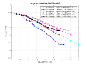
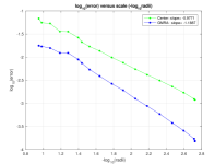
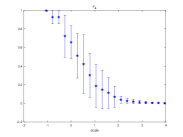
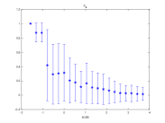
The log-log plot of the approximation error versus scale in Figure 5 (b) shows that volume measures on the $d$-dim S manifold are in $\mathcal{A}_{s}$ with $s\approx 2.0239,2.1372,2.173$ when $d=3,4,5$, consistent with our theory which gives $s=2$. Figure 5 (c) shows that volume measures on the $d$-dim Z manifold are in $\mathcal{A}_{s}$ with $s\approx 1.5367,1.6595,1.6204$ when $d=3,4,5$, consistent with our theory which gives $s=1.5$.

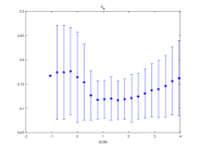
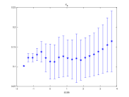
The log-log plot of the approximation error versus the weighted complexity of the adaptive partition in Figure 5 (d) and (e) gives rises to an approximation of the regularity parameter $s$ in the $\mathcal{B}_{s}$ model in the table.

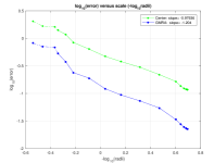
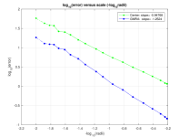
3.1.2 Error versus sample size $n$

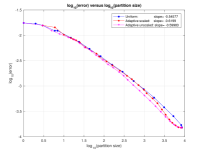
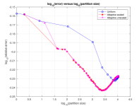
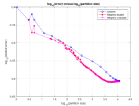
We take $n$ samples on the $4$-dim S and Z manifold. In Figure 6, we set the noise level $\sigma=0$ (a) and $\sigma=0.05$ (b), display the log-log plot of the average approximation error over 5 trails with respect to the sample size $n$ for empirical GMRA at scale $j^{*}$ which is chosen as per Theorem 4: $2^{-j^{*}}=[(\log n)/n]^{\frac{1}{2s+d-2}}$ with $d=4$ and $s=2$ for the S manifold and $s=1.5$ for the Z manifold. For adaptive GMRA, the ideal $\kappa$ increases as $\sigma$ increases. We let $\kappa\in\{0.05,0.1\}$ when $\sigma=0$ and $\kappa\in\{1,2\}$ when $\sigma=0.05$. We also test the Nearest Neighbor (NN) approximation. The negative of the slope, determined by least squared fit, gives rise to the rate of convergence: $L^{2}\ {\rm error}\sim(1/n)^{-\rm slope}$. When $\sigma=0$, the convergence rate for the nearest neighbor approximation should be $1/d=0.25$. GMRA gives rise to a smaller error and a faster rate of convergence than the nearest neighbor approximation. For the Z manifold, Adaptive GMRA yields a faster rate of convergence than GMRA. When $\sigma=0.05$, adaptive GMRA with $\kappa=0.5$ and $1$ gives rise to the fastest rate of convergence. Adaptive GMRA with $\kappa=0.05$ has similar rate of convergence as the nearest neighbor approximation since the tree is almost truncated at the finest scales. We note a de-noising effect when the approximation error falls below $\sigma$ as $n$ increases. In adaptive GMRA, when $\kappa$ is sufficiently large, i.e., $\kappa=0.5,1$ in this example, different values of $\kappa$ do yield different errors up to a constant, but the rate of convergence is independent of $\kappa$, as predicted by Theorem 8.

3.1.3 Robustness of GMRA and adaptive GMRA

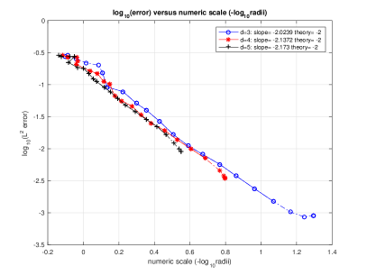
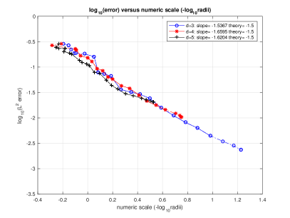
The robustness of the empirical GMRA and adaptive GMRA is tested on the $4$-dim S and Z manifold while $\sigma$ varies but $n$ is fixed to be $10^{5}$. Figure 7 shows that the average $L^{2}$ approximation error in $5$ trails increases linearly with respect to $\sigma$ for both uniform and adaptive GMRA with $\kappa\in\{0.05,0.5,1\}$.

(a) the $4$-dim S manifold, $\sigma=0$

(b) the $4$-dim S manifold, $\sigma=0.05$

(c) the $4$-dim Z manifold, $\sigma=0$

(d) the $4$-dim Z manifold, $\sigma=0.05$

Figure 6: $L^{2}$ error versus the sample size $n$, for the $4$-dim S and Z manifolds $(d=4)$, of GMRA at the scale $j^{*}$ chosen as per Theorem 4 and adaptive GMRA with varied $\kappa$. We let $\kappa\in\{0.05,0.1\}$ when $\sigma=0$ and $\kappa\in\{1,2\}$ when $\sigma=0.05$.

Figure 7: The average $L^{2}$ approximation error in $5$ trails versus $\sigma$ for GMRA and adaptive GMRA with $\kappa\in\{0.05,0.5,1\}$ on data sampled on the 4-dim S and Z manifolds. This shows the error of approximation grows linearly with the noise size, suggesting robustness in the construction.

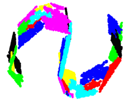
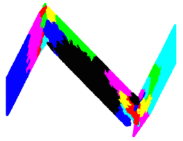
3.2 3D shapes

(a) 41,472 points

(b) 165,954 points

(c) 437,645 points

(d) $\kappa\approx 0.18$, partition size $=338$

(e) $\kappa\approx 0.41$, partition size $=749$

(f) $\kappa\approx 0.63$, partition size $=1141$

Figure 8: Top line: 3D shapes; bottom line: adaptive partitions selected with refinement criterion $\widehat{\Delta}_{j,k}\geq 2^{-j}\kappa\sqrt{(\log n)/n}$. Every cell is colored by scale. In the adaptive partition, at irregular locations cells are selected at finer scales than at “flat” locations.

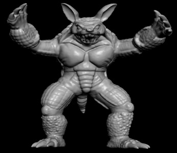
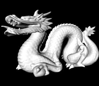
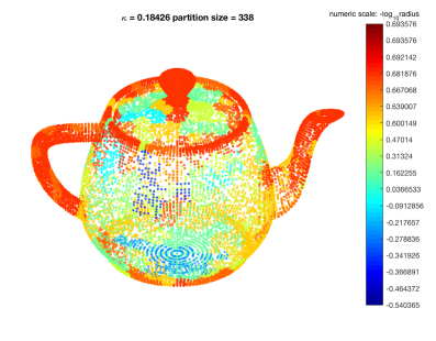
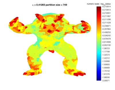
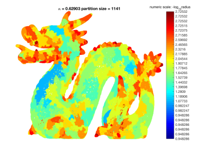
We run GMRA and adaptive GMRA on 3D points clouds on the teapot, armadillo and dragon in Figure 8. The teapot data are from the matlab toolbox and others are from the Stanford 3D Scanning Repository http://graphics.stanford.edu/data/3Dscanrep/.

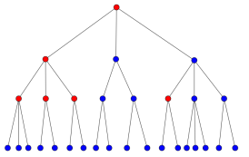
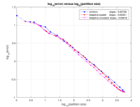
Figure 8 shows that the adaptive partitions chosen by adaptive GMRA matches our expectation that, at irregular locations, cells are selected at finer scales than at “flat” locations.

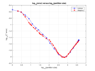
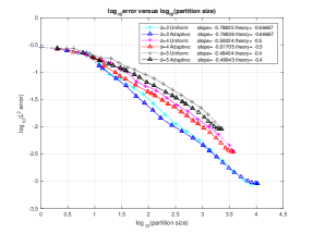
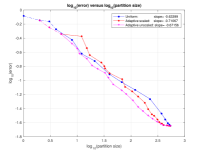
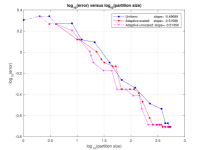
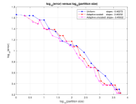
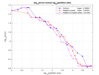
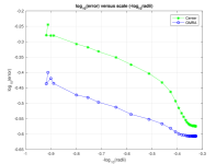
In Figure 9, we display the absolute $L^{2}/L^{\infty}$ approximation error on test data versus scale and partition size. The left column shows the $L^{2}$ approximation error versus scale for GMRA and the center approximation. While the GMRA approximation is piecewise linear, the center approximation is piecewise constant. Both approximation errors decay from coarse to fine scales, but GMRA yields a smaller error than the approximation by local centers. In the middle column, we run GMRA and adaptive GMRA with the $L^{2}$ refinement criterion defined in Table 2 with scale-dependent ($\Delta_{j,k}\geq 2^{-j}\tau_{n}$) and scale-independent ($\Delta_{j,k}\geq\tau_{n}$) threshold respectively, and display the log-log plot of the $L^{2}$ approximation error versus the partition size. Overall adaptive GMRA yields the same $L^{2}$ approximation error as GMRA with a smaller partition size, but the difference is insignificant in the armadillo and dragon, as these 3D shapes are complicated and the $L^{2}$ error simply averages the error at all locations. Then we implement adaptive GMRA with the $L^{\infty}$ refinement criterion: $\widehat{\Delta}_{j,k}^{\infty}=\max_{x_{i}\in C_{j,k}}\|\widehat{\mathcal{P}}_{j+1}x_{i}-\widehat{\mathcal{P}}_{j}x_{i}\|$ and display the log-log plot of the $L^{\infty}$ approximation error versus the partition size in the right column. In the $L^{\infty}$ error, adaptive GMRA saves a considerable number (about half) of cells in order to achieve the same approximation error as GMRA. In this experiment, scale-independent threshold is slightly better than scale-dependent threshold in terms of saving the partition size.

Teapot
Armadillo
Dragon

Figure 9: Left column: $\log_{10}(L^{2}$ error) versus scalefor GMRA and center approximation; Middle column: log-log plot of the $L^{2}$ error versus partition size for GMRA and adaptive GMRA with scale-dependent and scale-independent threshold under the $L^{2}$ refinement defined in Table 2; Right column: log-log plot of $L^{\infty}$ error versus partition size for GMRA and adaptive GMRA with scale-dependent and scale-independent threshold under the $L^{\infty}$ refinement.

(a) Scaling subspace

(b) $\log_{10}\|\widehat{\mathcal{P}}_{j+1}x_{i}-\widehat{\mathcal{P}}_{j}x_{i}\|$

(c) Error versus scale

(d) Error versus partition size

Figure 10: The top three rows: multiscale approximations of the digit $0,1,2$ in the MNIST data set, from the coarsest scale (left) to the finest scale (right). (a) the histogram of dimensions of the subspaces $\widehat{V}_{j,k}$; (b) $\log_{10}\|\widehat{\mathcal{P}}_{j+1}x_{i}-\widehat{\mathcal{P}}_{j}x_{i}\|$ from the coarsest scale (top) to the finest scale (bottom), with columns indexed by the digits, sorted from $0$ to $9$; (c) log-log plot of the relative $L^{2}$ error versus scale in GMRA and the center approximation; (d) log-log plot of the relative $L^{2}$ error versus partition size for GMRA, adaptive GMRA with scale-dependent and scale-independent threshold.

3.3 MNIST digit data

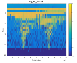
We consider the MNIST data set from http://yann.lecun.com/exdb/mnist/, which contains images of $60,000$ handwritten digits, each of size $28\times 28$, grayscale. The intrinsic dimension of this data set varies for different digits and across scales, as it was observed in Little et al. (2012). We run GMRA by setting the diameter of cells at scale $j$ to be $\mathcal{O}(0.9^{j})$ in order to slowly zoom into the data at multiple scales.

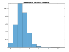
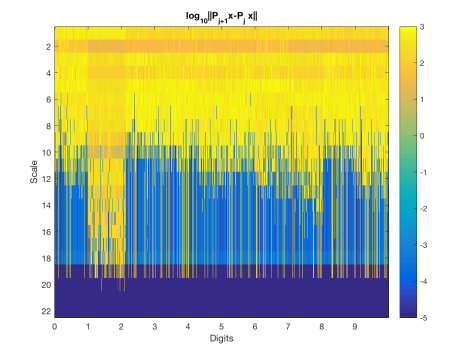
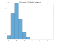
We evenly split the digits to the training set and the test set. As the intrinsic dimension is not well-defined, we set GMRA to pick the dimension of $\widehat{V}_{j,k}$ adaptively, as the smallest dimension needed to capture $50\%$ of the energy of the data in $C_{j,k}$. As an example, we display the GMRA approximations of the digit $0,1,2$ from coarse scales to fine scales in Figure 10. The histogram of the dimensions of the subspaces $\widehat{V}_{j,k}$ is displayed in (a). (b) represents $\log_{10}\|\widehat{\mathcal{P}}_{j+1}x_{i}-\widehat{\mathcal{P}}_{j}x_{i}\|$ from the coarsest scale (top) to the finest scale (bottom), with columns indexed by the digits, sorted from $0$ to $9$. We observe that $1$ has more fine scale information than the other digits. In (c), we display the log-log plot of the relative $L^{2}$ error versus scale in GMRA and the center approximation. The improvement of GMRA over center approximation is noticeable. Then we compute the relative $L^{2}$ error for GMRA and adaptive GMRA when the partition size varies. Figure 10 (d) shows that adaptive GMRA achieves the same accuracy as GMRA with fewer cells in the partition. Errors increase when the partition size exceeds $10^{3}$ due to a large variance at fine scales. In this experiment, scale-dependent threshold and scale-independent threshold yield similar performances.

Learning image patches

Learning the Fourier magnitudes of image patches

(a) Scaling subspace

(b) Error versus scale

(c) Error versus partition size

(d) Scaling subspace

(e) Error versus scale

(f) Error versus partition size

Figure 11: Caltech 101 image patches

Figure 12: Top line: learning on $200,000$ image patches; bottom line: results of learning the Fourier magnitudes of the same image patches. (a,d) histograms of the dimensions of the subspaces $\widehat{V}_{j,k}$; (b,e) relative $L^{2}$ error versus scale for GMRA and the center approximation; (c,f) relative $L^{2}$ error versus the partition size for GMRA, adaptive GMRA with scale-dependent and scale-independent threshold.

3.4 Natural image patches

It was argued in Peyré (2009) that many sets of patches extracted from natural images can be modeled a low-dimensional manifold. We use the Caltech 101 dataset from https://www.vision.caltech.edu/Image_Datasets/Caltech101/ (see F. Li and Perona, 2006), take 40 images from four categories: accordion, airplanes, hedgehog and scissors and extract multiscale patches of size $8\times 8$ from these images. Specifically, if the image is of size $m\times m$, for $\ell=1,\ldots,\log_{2}(m/8)$, we collect patches of size $2^{\ell}8$, low-pass filter them and downsample them to become patches of size $8\times 8$ (see Gerber and Maggioni (2013) for a discussion about dictionary learning on patches of multiple sizes using multiscale ideas). Then we randomly pick $200,000$ patches, evenly split them to the training set and the test set. In the construction of GMRA, we set the diameter of cells at scale $j$ to be $\mathcal{O}(0.9^{j})$ and the dimension of $\widehat{V}_{j,k}$ to be the smallest dimension needed to capture $50\%$ of the energy of the data in $C_{j,k}$. We also run GMRA and adaptive GMRA on the Fourier magnitudes of these image patches to take advantage of translation-invariance of the Fourier magnitudes. The results are shown in Figure 12. The histograms of the dimensions of the subspaces $\widehat{V}_{j,k}$ are displayed in (a,e). Figure 12 (c) and (g) show the relative $L^{2}$ error versus scale for GMRA and the center approximation. We then compute the relative $L^{2}$ error for GMRA and adaptive GMRA when the partition size varies and display the log-log plot in (d) and (h). It is noticeable that adaptive GMRA achieves the same accuracy as GMRA with a smaller partition size. We conducted similar experiments on $200,000$ multiscale patches from CIFAR 10 from https://www.cs.toronto.edu/~kriz/cifar.html (see Krizhevsky and Hinton, 2009) with extremely similar results (not shown).

4 Performance analysis of GMRA and adaptive GMRA

This section is devoted to the performance analysis of empirical GMRA and adaptive GMRA. We will start with the following stochastic error estimate on any partition.

4.1 Stochastic error on a fixed partition

Suppose $\tilde{\mathcal{T}}$ is a finite proper subtree of the data master tree $\mathcal{T}^{n}$. Let $\Lambda$ be the partition consisting the outer leaves of $\tilde{\mathcal{T}}$. The piecewise affine projector on $\Lambda$ and its empirical version are

$$\mathcal{P}_{\Lambda}=\sum_{C_{j,k}\in\Lambda}\mathcal{P}_{j,k}\mathbf{1}_{j,k}\quad\text{and}\quad\widehat{\mathcal{P}}_{\Lambda}=\sum_{C_{j,k}\in\Lambda}\widehat{\mathcal{P}}_{j,k}\mathbf{1}_{j,k}.$$

A non-asymptotic probability bound on the stochastic error $\|\mathcal{P}_{\Lambda}X-\widehat{\mathcal{P}}_{\Lambda}X\|$ is given by:

Lemma 14

Let $\Lambda$ be the partition associated a finite proper subtree $\tilde{\mathcal{T}}$ of the data master tree $\mathcal{T}^{n}$. Suppose $\Lambda$ contains $\#_{j}\Lambda$ cells at scale $j$. Then for any $\eta>0$,

$$\mathbb{P}\{\|\mathcal{P}_{\Lambda}X-\widehat{\mathcal{P}}_{\Lambda}X\|\geq\eta\}\leq\alpha d\cdot\#\Lambda\cdot e^{-\frac{\beta n\eta^{2}}{d^{2}\sum_{j}2^{-2j}\#_{j}\Lambda}}$$ (17)

$$\mathbb{E}\|\mathcal{P}_{\Lambda}X-\widehat{\mathcal{P}}_{\Lambda}X\|^{2}\leq\frac{d^{2}\log(\alpha d\#\Lambda)\sum_{j}2^{-2j}\#_{j}\Lambda}{\beta n}$$

where $\alpha=\alpha(\theta_{2},\theta_{3})$ and $\beta=\beta(\theta_{2},\theta_{3},\theta_{4})$.

Lemma 14 and Proposition 15 below are proved in appendix C .

4.2 Performance analysis of empirical GMRA

According to Eq. (1), the approximation error of empirical GMRA is split into the squared bias and the variance. A corollary of Lemma 14 with $\Lambda=\Lambda_{j}$ results in an estimate of the variance term.

Proposition 15

For any $\eta\geq 0$,

$$\mathbb{P}\{\|\mathcal{P}_{j}X-\widehat{\mathcal{P}}_{j}X\|\geq\eta\} \leq \alpha d\#\Lambda_{j}e^{-\frac{\beta 2^{2j}n\eta^{2}}{d^{2}\#\Lambda_{j}}}$$ (18)

$$\mathbb{E}\|\mathcal{P}_{j}X-\widehat{\mathcal{P}}_{j}X\|^{2} \leq \frac{d^{2}\#\Lambda_{j}\log[\alpha d\#\Lambda_{j}]}{\beta 2^{2j}n}\,.$$ (19)

In Eq. (1), the squared bias decays like $\mathcal{O}(2^{-2js})$ whenever $\rho\in\mathcal{A}_{s}$ and the variance scales like $\mathcal{O}(j2^{j(d-2)}/n)$. A proper choice of the scale $j$ gives rise to Theorem 4 whose proof is given below.

Proof of Theorem 4

Proof [Proof of Theorem 4]

$$\mathbb{E}\|X-\widehat{\mathcal{P}}_{j}X\|^{2}\leq\|X-\mathcal{P}_{j}X\|^{2}+\mathbb{E}\|\mathcal{P}_{j}X-\widehat{\mathcal{P}}_{j}X\|^{2}$$

$$\leq|\rho|_{\mathcal{A}_{s}}^{2}2^{-2sj}+\frac{d^{2}\#\Lambda_{j}\log[\alpha d\#\Lambda_{j}]}{\beta 2^{2j}n}\leq|\rho|_{\mathcal{A}_{s}}^{2}2^{-2sj}+\frac{d^{2}2^{j(d-2)}}{\theta_{1}\beta n}\log\frac{\alpha d2^{jd}}{\theta_{1}}$$

as $\#\Lambda_{j}\leq 2^{jd}/\theta_{1}$ due to Assumption (A3).

Intrinsic dimension $d=1$: In this case, both the squared bias and the variance decrease as $j$ increases, so we should choose the scale $j^{*}$ as large as possible as long as most cells at scale $j^{*}$ have $d$ points. We will choose $j^{*}$ such that $2^{-j^{*}}=\mu\frac{\log n}{n}$ for some $\mu>0$. After grouping $\Lambda_{j^{*}}$ into light and heavy cells whose measure is below or above $\frac{28(\nu+1)\log n}{3n}$, we can show that the error on light cells is upper bounded by $C(\frac{\log n}{n})^{2}$ and all heavy cells have at least $d$ points with high probability.

Lemma 16

Suppose $j^{*}$ is chosen such that $2^{-j^{*}}=\mu\frac{\log n}{n}$ with some $\mu>0$. Then

$$\|(X-\mathcal{P}_{j^{*}}X)\mathbf{1}_{\{C_{j^{*},k}:\rho(C_{j^{*},k})\leq\frac{28(\nu+1)\log n}{3n}\}}\|^{2}\leq\frac{28(\nu+1)\theta_{2}^{2}\mu}{3\theta_{1}}\left(\frac{\log n}{n}\right)^{2},$$

$$\mathbb{P}\left\{\text{each }C_{j^{*},k}\text{ satisfying }\rho(C_{j^{*},k})>\tfrac{28(\nu+1)\log n}{3n}\text{ has at least $d$ points}\right\}\geq 1-n^{-\nu}.$$

Lemma 16 is proved in appendix D. If $j^{*}$ is chosen as above, The probability estimate in (5) follows from

$$\|X-\mathcal{P}_{j^{*}}X\|\leq|\rho|_{\mathcal{A}_{s}}2^{-sj^{*}}\leq|\rho|_{\mathcal{A}_{s}}\mu^{s}\left(\frac{\log n}{n}\right)^{s}\leq|\rho|_{\mathcal{A}_{s}}\mu^{s}\frac{\log n}{n},$$

$$\mathbb{P}\left\{\|\mathcal{P}_{j^{*}}X-\widehat{\mathcal{P}}_{j^{*}}X\|\geq C_{1}\frac{\log n}{n}\right\}\leq\tfrac{\alpha}{\theta_{1}\mu}\left((\log n)/n\right)^{-1}e^{-\frac{{\mu\beta\theta_{1}C_{1}^{2}}\log n}{d^{2}}}\leq\tfrac{\alpha}{\theta_{1}\mu}\frac{n\,n^{-\frac{\mu\beta\theta_{1}C_{1}^{2}}{d^{2}}}}{\log n}\leq C_{2}n^{-\nu}\,$$

provided that ${\mu\beta\theta_{1}C_{1}^{2}/d^{2}}-1>\nu$.

Intrinsic dimension $d\geq 2$: When $d\geq 2$, the squared bias decreases but the variance increases as $j$ gets large. We choose $j^{*}$ such that $2^{-j^{*}}=\mu\left((\log n)/n\right)^{\frac{1}{2s+d-2}}$ to balance these two terms. We use the same technique as $d=1$ to group $\Lambda_{j^{*}}$ into light and heavy cells whose measure is below or above $28/3\cdot(\nu+1)(\log n)/n$, we can show that the error on light cells is upper bounded by $C((\log n)/n)^{\frac{2s}{2s+d-2}}$ and all heavy cells have at least $d$ points with high probability.

Lemma 17

Let $j^{*}$ be chosen such that $2^{-j^{*}}=\mu\left((\log n)/n\right)^{\frac{1}{2s+d-2}}$ with some $\mu>0$. Then

$$\|(X-\mathcal{P}_{j^{*}}X)\mathbf{1}_{\{C_{j^{*},k}:\rho(C_{j^{*},k})\leq\frac{28(\nu+1)\log n}{3n}\}}\|^{2}\leq\frac{28(\nu+1)\theta_{2}^{2}\mu^{2-d}}{3\theta_{1}}\left(\frac{\log n}{n}\right)^{\frac{2s}{2s+d-2}},$$

$$\mathbb{P}\left\{\forall\,C_{j^{*},k}\,:\,\rho(C_{j^{*},k})>\frac{28(\nu+1)\log n}{3n},\,\,C_{j^{*},k}\text{ has at least $d$ points}\right\}\geq 1-n^{-\nu}.$$

Proof of Lemma 17 is omitted since it is the same as the proof of Lemma 16. The probability estimate in (6) follows from

$$\|X-\mathcal{P}_{j^{*}}X\|\leq|\rho|_{\mathcal{A}_{s}}2^{-s{j^{*}}}\leq|\rho|_{\mathcal{A}_{s}}\mu^{s}\left(\frac{\log n}{n}\right)^{\frac{s}{2s+d-2}},$$

$$\mathbb{P}\left\{\|\mathcal{P}_{j^{*}}X-\widehat{\mathcal{P}}_{j^{*}}X\|\geq C_{1}\left(\frac{\log n}{n}\right)^{\frac{s}{2s+d-2}}\right\}\leq\frac{\alpha d\mu^{-d}}{\theta_{1}}\left(\frac{\log n}{n}\right)^{-\frac{d}{2s+d-2}}e^{-\frac{\beta\theta_{1}C_{1}^{2}\mu^{d-2}\log n}{d^{2}}}\leq C_{2}n^{-\nu}$$

provided that ${\beta\theta_{1}C_{1}^{2}\mu^{d-2}}/d^{2}-1>\nu$.

 

4.3 Performance analysis of Adaptive GMRA

Proof [Proof of Theorem 8] In the case that $\mathcal{M}$ is bounded by $M$, the minimum scale $j_{\rm min}=\log_{2}\frac{\theta_{2}}{M}$. We first consider the case $d\geq 3$. In our proof $C$ stands for constants that may vary at different locations, but it is independent of $n$ and $D$. We will begin by defining several objects of interest:

• $\mathcal{T}^{n}$: the data master tree whose leaf contains at least $d$ points in $\mathcal{X}_{n}$. It can be viewed as the part of a multiscale tree that our data have explored.

• $\mathcal{T}$: a complete multiscale tree containing $\mathcal{T}^{n}$. $\mathcal{T}$ can be viewed as the union $\mathcal{T}^{n}$ and some empty cells, mostly at fine scales with high probability, that our data have not explored.

• $\mathcal{T}_{(\rho,\eta)}$: the smallest subtree of $\mathcal{T}$ which contains $\{C_{j,k}\in\mathcal{T}\,:\,\Delta_{j,k}\geq 2^{-j}\eta\}$.

• $\mathcal{T}_{\eta}=\mathcal{T}_{(\rho,\eta)}\cap\mathcal{T}^{n}$.

• $\widehat{\mathcal{T}}_{\eta}$: the smallest subtree of $\mathcal{T}^{n}$ which contains $\{C_{j,k}\in\mathcal{T}^{n}\,:\,\widehat{\Delta}_{j,k}\geq 2^{-j}\eta\}$.

• $\Lambda_{(\rho,\eta)}$: the partition associated with $\mathcal{T}_{(\rho,\eta)}$.

• $\Lambda_{\eta}:$ the partition associated with $\mathcal{T}_{\eta}$.

• $\widehat{\Lambda}_{\eta}:$ the partition associated with $\widehat{\mathcal{T}}_{\eta}$.

• Suppose $\mathcal{T}^{0}$ and $\mathcal{T}^{1}$ are two subtrees of $\mathcal{T}$. If $\Lambda^{0}$ and ${\Lambda}^{1}$ are two adaptive partitions associated with $\mathcal{T}^{0}$ and $\mathcal{T}^{1}$ respectively, we denote by $\Lambda^{0}\vee\Lambda^{1}$ and $\Lambda^{0}\wedge\Lambda^{1}$ the partitions associated to the trees $\mathcal{T}^{0}\cup\mathcal{T}^{1}$ and $\mathcal{T}^{0}\cap\mathcal{T}^{1}$ respectively.

We also let $b=2a_{\rm max}+5$ where $a_{\rm max}$ is the maximal number of children that a node has in $\mathcal{T}$; $\kappa_{0}=\max(\kappa_{1},\kappa_{2})$ where ${b^{2}\kappa_{1}^{2}}/(21\theta_{2}^{2})=\nu+1$ and $\alpha_{2}\kappa_{2}^{2}/b^{2}=\nu+1$ with $\alpha_{2}$ defined in Lemma 19. In order the obtain the MSE bound, one can simply set $\nu=1$.

The empirical adaptive GMRA projection is given by $\widehat{\mathcal{P}}_{\widehat{\Lambda}_{\tau_{n}}}=\sum_{C_{j,k}\in\widehat{\Lambda}_{\tau_{n}}}\widehat{\mathcal{P}}_{j,k}\mathbf{1}_{j,k}.$ Using the triangle inequality, we split the error as follows:

$$\|X-\widehat{\mathcal{P}}_{\widehat{\Lambda}_{\tau_{n}}}X\|\leq e_{1}+e_{2}+e_{3}+e_{4}$$

where

$$e_{1} :=\|X-\mathcal{P}_{\widehat{\Lambda}_{\tau_{n}}\vee\Lambda_{b\tau_{n}}}X\|\,, e_{2} :=\|\mathcal{P}_{\widehat{\Lambda}_{\tau_{n}}\vee\Lambda_{b\tau_{n}}}X-\mathcal{P}_{\widehat{\Lambda}_{\tau_{n}}\wedge\Lambda_{\tau_{n}/b}}X\|$$

$$e_{3} :=\|\mathcal{P}_{\widehat{\Lambda}_{\tau_{n}}\wedge\Lambda_{\tau_{n}/b}}X-\widehat{\mathcal{P}}_{\widehat{\Lambda}_{\tau_{n}}\wedge\Lambda_{\tau_{n}/b}}X\|\,, e_{4} :=\|\widehat{\mathcal{P}}_{\widehat{\Lambda}_{\tau_{n}}\wedge\Lambda_{\tau_{n}/b}}X-\widehat{\mathcal{P}}_{\widehat{\Lambda}_{\tau_{n}}}X\|.$$

A similar split appears in the works of Binev et al. (2005, 2007). The partition built from those $C_{j,k}$’s satisfying $\widehat{\Delta}_{j,k}\geq 2^{-j}\tau_{n}$ does not exactly coincide with the partition chosen based on those $C_{j,k}$ satisfying $\Delta_{j,k}\geq 2^{-j}\tau_{n}$. This is accounted by $e_{2}$ and $e_{4}$, corresponding to those $C_{j,k}$’s whose $\widehat{\Delta}_{j,k}$ is significantly larger or smaller than $\Delta_{j,k}$, which we will prove to be small with high probability. The remaining terms $e_{1}$ and $e_{3}$ correspond to the bias and variance of the approximations on the partition obtained by thresholding $\Delta_{j,k}$.

Term $e_{1}$: The first term $e_{1}$ is essentially the bias term. Since $\widehat{\Lambda}_{\tau_{n}}\vee\Lambda_{b\tau_{n}}\supseteq\Lambda_{b\tau_{n}}$,

$$e_{1}^{2} =\|X-\mathcal{P}_{\widehat{\Lambda}_{\tau_{n}}\vee\Lambda_{b\tau_{n}}}X\|^{2}\leq\|X-\mathcal{P}_{\Lambda_{b\tau_{n}}}X\|^{2}\leq\underbrace{\|X-\mathcal{P}_{\Lambda_{(\rho,b\tau_{n})}}X\|^{2}}_{e_{11}^{2}}+\underbrace{\|\mathcal{P}_{\Lambda_{(\rho,b\tau_{n})}}X-\mathcal{P}_{\Lambda_{b\tau_{n}}}X\|^{2}}_{e_{12}^{2}}\,.$$

$e_{11}^{2}$ may be upper bounded deterministically from Eq. (9):

$$e_{11}^{2}\leq B_{s,d}|\rho|_{\mathcal{B}_{s}}^{p}(b\tau_{n})^{2-p}\leq B_{s,d}|\rho|_{\mathcal{B}_{s}}^{\frac{2(d-2)}{2s+d-2}}(b\kappa)^{\frac{4s}{2s+d-2}}\left(\frac{\log n}{n}\right)^{\frac{2s}{2s+d-2}}.$$ (20)

$e_{12}$ encodes the difference between thresholding $\mathcal{T}$ and $\mathcal{T}^{n}$, but it is $0$ with high probability:

Lemma 18

For any $\nu>0$, $\kappa$ such that $\kappa>\kappa_{1}$, where $b^{2}\kappa_{1}^{2}/(21\theta_{2}^{2})=\nu+1$,

$$\mathbb{P}\{e_{12}>0\}\leq C(\theta_{2},a_{\rm max},a_{\rm min},\kappa)n^{-\nu}$$ (21)

The proof is postponed, together with those of the Lemmata that follow, to appendix D). If $\mathcal{M}$ is bounded by $M$, then $e_{12}^{2}\leq 4M^{2}$ and

$$\mathbb{E}e_{12}^{2}\leq 4M^{2}\mathbb{P}\{e_{12}>0\}\leq 4M^{2}Cn^{-{\nu}}\leq 4M^{2}C\left(\frac{\log n}{n}\right)^{\frac{2s}{2s+d-2}}$$ (22)

if ${\nu}>{2s}/(2s+d-2)$, for example ${\nu}=1$.

Term $e_{3}$: $e_{3}$ corresponds to the variance on the partition $\widehat{\Lambda}_{\tau_{n}}\wedge\Lambda_{\tau_{n}/b}$. For any $\eta>0$,

$$\mathbb{P}\{e_{3}>\eta\}\leq\alpha d\#(\widehat{\Lambda}_{\tau_{n}}\wedge\Lambda_{\tau_{n}/b})e^{-\frac{\beta n\eta^{2}}{d^{2}\sum_{j\geq j_{\rm min}}2^{-2j}\#_{j}(\widehat{\Lambda}_{\tau_{n}}\wedge\Lambda_{\tau_{n}/b})}}$$

according to Lemma 14. Since $\widehat{\Lambda}_{\tau_{n}}\wedge\Lambda_{\tau_{n}/b}\subset\mathcal{T}_{\tau_{n}/b}$, for any $j\geq 0$, regardless of $\widehat{\Lambda}_{\tau_{n}}$, we have $\#_{j}(\widehat{\Lambda}_{\tau_{n}}\wedge\Lambda_{\tau_{n}/b})\leq\#_{j}\mathcal{T}_{\tau_{n}/b}\leq\#\mathcal{T}_{\tau_{n}/b}$. Therefore

$$\mathbb{P}\{e_{3}>\eta\} \leq\alpha d\#\mathcal{T}_{\tau_{n}/b}e^{-\frac{\beta n\eta^{2}}{d^{2}\sum_{j\geq j_{\rm min}}2^{-2j}\#_{j}\mathcal{T}_{\tau_{n}/b}}}\leq\alpha d\#\mathcal{T}_{\tau_{n}/b}e^{-\frac{\beta n\eta^{2}}{d^{2}|\rho|_{\mathcal{B}_{s}}^{p}(\tau_{n}/b)^{-p}}}\,,$$ (23)

which implies

$$\mathbb{E}e_{3}^{2}=\int_{0}^{+\infty}\eta\mathbb{P}\left\{e_{3}>\eta\right\}d\eta=\int_{0}^{+\infty}\eta\min\left(1,\alpha d\#\mathcal{T}_{\tau_{n}/b}e^{-\frac{\beta n\eta^{2}}{d^{2}\sum_{j\geq j_{\rm min}}2^{-2j}\#_{j}\mathcal{T}_{\tau_{n}/b}}}\right)d\eta$$

$$\leq\frac{d^{2}\log\alpha d\#\mathcal{T}_{\tau_{n}/b}}{\beta n}\!\sum_{j\geq j_{\rm min}}2^{-2j}\#_{j}\mathcal{T}_{\tau_{n}/b}\leq C\frac{\log n}{n}\left(\frac{\tau_{n}}{b}\right)^{-p}\!\!\leq C(\theta_{2},\theta_{3},d,\kappa,s,|\rho|_{\mathcal{B}_{s}})\left(\frac{\log n}{n}\right)^{\frac{2s}{2s+d-2}}\!\!\!\!\!\!\!\!\!\!.$$

Term $e_{2}$ and $e_{4}$: These terms account for the difference of truncating the master tree based on $\Delta_{j,k}$’s and its empirical counterparts $\widehat{\Delta}_{j,k}$’s. We prove that $\widehat{\Delta}_{j,k}$’s concentrate near $\Delta_{j,k}$’s with high probability if there are sufficient samples.

Lemma 19

For any $\eta>0$ and any $C_{j,k}\in\mathcal{T}$

$$\max\left\{\mathbb{P}\left\{\widehat{\Delta}_{j,k}\leq\eta\ \text{ and }\ \Delta_{j,k}\geq b\eta\right\},\mathbb{P}\left\{\Delta_{j,k}\leq\eta\ \text{ and }\ \widehat{\Delta}_{j,k}\geq b\eta\right\}\right\} \leq\alpha_{1}e^{-\alpha_{2}2^{2j}n\eta^{2}}$$ (24)

for some constants $\alpha_{1}:=\alpha_{1}(\theta_{2},\theta_{3},a_{\rm max},d)$ and $\alpha_{2}:=\alpha_{2}(\theta_{2},\theta_{3},\theta_{4},a_{\rm max},d)$.

This Lemma enables one to show that $e_{2}=0$ and $e_{4}=0$ with high probability:

Lemma 20

Let $\alpha_{1}$ and $\alpha_{2}$ be the constants in Lemma 19. For any fixed ${\nu}>0$,

$$\mathbb{P}\{e_{2}>0\}+\mathbb{P}\{e_{4}>0\}\leq\alpha_{1}a_{\rm min}n^{-{\nu}}$$ (25)

when $\kappa$ is chosen such that $\kappa>\kappa_{2}$, with $\alpha_{2}\kappa_{2}^{2}/b^{2}={\nu}+1$.

Since $\mathcal{M}$ is bounded by $M$, we have $e_{2}^{2}\leq 4M^{2}$ so

$$\mathbb{E}e_{2}^{2}\leq 4M^{2}\mathbb{P}\{e_{2}>0\}\leq 4M^{2}\alpha_{1}a_{\rm min}n^{-{\nu}}\leq 4M^{2}\alpha_{1}a_{\rm min}\left(\frac{\log n}{n}\right)^{\frac{2s}{2s+d-2}}$$

if ${\nu}>{2s}/(2s+d-2)$, for example ${\nu}=1$. The same bound holds for $e_{4}$.

Finally, we complete the probability estimate (10): let $c_{0}^{2}=B_{s,d}|\rho|_{\mathcal{B}_{s}}^{\frac{2(d-2)}{2s+d-2}}(b\kappa)^{\frac{4s}{2s+d-2}}$ such that $e_{11}\leq c_{0}\left((\log n)/n\right)^{\frac{s}{2s+d-2}}$. We have

$$\mathbb{P}\left\{\|X-\widehat{\mathcal{P}}_{\widehat{\Lambda}_{\tau_{n}}}X\|\geq c_{1}\left((\log n)/n\right)^{\frac{s}{2s+d-2}}\right\}$$

$$\leq\mathbb{P}\left\{e_{3}>(c_{1}-c_{0})\left((\log n)/n\right)^{\frac{s}{2s+d-2}}\right\}+\mathbb{P}\{e_{12}>0\}+\mathbb{P}\{e_{2}>0\}+\mathbb{P}\{e_{4}>0\}$$

$$\leq\mathbb{P}\left\{e_{3}>(c_{1}-c_{0})\left((\log n)/n\right)^{\frac{s}{2s+d-2}}\right\}+Cn^{-{\nu}},$$

as long as $\kappa$ is chosen such that $\kappa>\max(\kappa_{1},\kappa_{2})$ where ${b^{2}\kappa_{1}^{2}}/(21\theta_{2}^{2})=\nu+1$ and $\alpha_{2}\kappa_{2}^{2}/b^{2}=\nu+1$ according to (21) and (25). Applying (23) gives rise to

$$\mathbb{P}\left\{e_{3}>(c_{1}-c_{0})\left((\log n)/n\right)^{\frac{s}{2s+d-2}}\right\}\leq\alpha d\#\mathcal{T}_{\tau_{n}/b}e^{-\frac{\beta n}{|\rho|_{\mathcal{B}_{s}}^{p}(\tau_{n}/b)^{-p}}(c_{1}-c_{0})^{2}\left((\log n)/n\right)^{\frac{2s}{2s+d-2}}}$$

$$\leq\alpha d\#\mathcal{T}_{\tau_{n}/b}n^{-\frac{\beta(c_{1}-c_{0})^{2}\kappa^{p}}{b^{p}|\rho|_{\mathcal{B}_{s}}^{p}}}\leq\alpha da_{\rm min}n^{-\left(\frac{\beta(c_{1}-c_{0})^{2}\kappa^{p}}{b^{p}|\rho|_{\mathcal{B}_{s}}^{p}}-1\right)}\leq\alpha da_{\rm min}n^{-{\nu}}$$

if $c_{1}$ is taken large enough such that $\frac{\beta(c_{1}-c_{0})^{2}\kappa^{p}}{b^{p}|\rho|_{\mathcal{B}_{s}}^{p}}\geq{\nu}+1$.

We are left with the cases $d=1,2$. When $d=1$, for any distribution $\rho$ satisfying quasi-orthogonality (8) and any $\eta>0$, the tree complexity may be bounded as follows:

$$\sum_{j\geq j_{\rm min}}2^{-2j}\#_{j}\mathcal{T}_{(\rho,\eta)}\leq\sum_{j\geq j_{\rm min}}2^{-2j}2^{j}/\theta_{1}=2/\theta_{1}2^{-j_{\rm min}}=2M/(\theta_{1}\theta_{2})\,,$$

so $\|X-\mathcal{P}_{\Lambda_{(\rho,\eta)}}X\|^{2}\leq 8MB_{0}\eta^{2}/(3\theta_{1}\theta_{2})$. Hence

$$e_{11}^{2}\leq\tfrac{8MB_{0}}{3\theta_{1}\theta_{2}}(b\tau_{n})^{2}\leq\tfrac{8MB_{0}b^{2}\kappa^{2}}{3\theta_{1}\theta_{2}}(\log n)/n,\quad\mathbb{P}\{e_{3}>\eta\}\leq\alpha d\#\mathcal{T}_{\tau_{n}/b}e^{-\frac{\theta_{1}\theta_{2}\beta n\eta^{2}}{2Md^{2}}},$$

which yield $\mathbb{E}e_{3}^{2}\leq 2Md^{2}\log\alpha d\#\mathcal{T}_{\tau_{n}/b}/(\theta_{1}\theta_{2}\beta n)\leq C(\log n)/n$ and estimate (11).

When $d=2$, for any distribution satisfying quasi-orthogonality and given any $\eta>0$, we have $\sum_{j\geq j_{\rm min}}2^{-2j}\#_{j}\mathcal{T}_{(\rho,\eta)}\leq-|\rho|^{-1}\log\eta$, whence $\|X-\mathcal{P}_{\Lambda_{(\rho,\eta)}}X\|^{2}\leq-\frac{4}{3}B_{0}|\rho|\eta^{2}\log\eta$. Therefore

$$e_{11}^{2}\leq-\tfrac{4}{3}B_{0}|\rho|(b\tau_{n})^{2}\log(b\tau_{n})\leq C(\log^{2}n)/n\quad,\quad\mathbb{P}\{e_{3}>\eta\}\leq\alpha d\#\mathcal{T}_{\tau_{n}/b}e^{-\frac{2\beta n\eta^{2}}{d^{2}|\rho|\log n}}\,,$$

which yield $\mathbb{E}e_{3}^{2}\leq d^{2}|\rho|\log\alpha d\#\mathcal{T}_{\tau_{n}/b}(\log n)/(2\beta n)\leq C(\log^{2}n)/n$ and the probability estimate (12).  

Proof [Proof of Theorem 9] Let $R>0$. If we run adaptive GMRA on $B_{R}(0)$, and approximate points outside $B_{R}(0)$ by $0$, the MSE of the adaptive GMRA in $B_{R}(0)$ is

$$\|(\mathbb{I}-\widehat{\mathcal{P}}_{\widehat{\Lambda}_{\tau_{n}}})\mathbf{1}_{\{\|x\|\leq R\}}X\|^{2}\lesssim(\Large|\rho|_{B_{\mathbf{0}}(R)}\Large|^{p}+R^{2})\left((\log n)/n\right)^{\frac{2s}{2s+d-2}}\lesssim R^{\max(\lambda,2)}\left((\log n)/n\right)^{\frac{2s}{2s+d-2}}.$$

The squared error outside $B_{R}(0)$ is

$$\|\mathbf{1}_{\{\|x\|\geq R\}}X\|^{2}=\int_{B_{R}(0)^{c}}||x||^{2}d\rho\leq CR^{-\delta}.$$ (26)

The total MSE is

$${\rm MSE}\lesssim R^{\max(\lambda,2)}\left((\log n)/n\right)^{\frac{2s}{2s+d-2}}+R^{-\delta}.$$

Minimizing over $R$ suggests taking $R=R_{n}=\max(R_{0},\mu(\log n/n)^{-\frac{2s}{(2s+d-2)(\delta+\max(2,\lambda))}})$, yielding ${\rm MSE}\lesssim\left((\log n)/n\right)^{\frac{2s}{2s+d-2}\cdot\frac{\delta}{\delta+\max(\lambda,2)}}.$ The probability estimate (13) follows from Eq. (26) and Eq. (10) in Theorem 8.  

In Remark 10, we claim that $\lambda$ is not large in simple cases. If $\rho\in\mathcal{A}_{s}^{\infty}$ and $\rho$ decays such that $\rho(C_{j,k})\leq 2^{-jd}\|c_{j,k}\|^{-(d+1+\delta)}$, we have $\Delta_{j,k}\leq 2^{-js}2^{-jd/2}\|c_{j,k}\|^{-(d+1+\delta)/2}$. Roughly speaking, for any $\eta>0$, the cells of distance $r$ to $0$ satisfying $\Delta_{j,k}\geq 2^{-j}\eta$ will satisfy $2^{-j}\geq(\eta r^{\frac{d+1+\delta}{2}})^{\frac{2}{2s+d-2}}$. In other words, the cells of distance $r$ to $0$ are truncated at scale $j_{\rm max}$ such that $2^{-j_{\rm max}}=(\eta r^{\frac{d+1+\delta}{2}})^{\frac{2}{2s+d-2}}$, which gives rise to complexity $\leq 2^{-2j_{\rm max}}r^{d-1}2^{j_{\rm max}d}\leq\eta^{-\frac{2(d-2)}{2s+d-2}}r^{d-1-\frac{(d+1+\delta)(d-2)}{2s+d-2}}$. If we run adaptive GMRA with threshold $\eta$ on $B_{R}(0)$, the weighted complexity of the truncated tree is upper bounded by $\eta^{-\frac{2(d-2)}{2s+d-2}}r^{d-\frac{(d+1+\delta)(d-2)}{2s+d-2}}$. Therefore, $\rho|_{B_{R}(0)}\in\mathcal{B}_{s}$ for all $R>0$ and $\Large|\rho|_{B_{R}(0)}\Large|_{\mathcal{B}_{s}}^{p}\leq R^{\lambda}$ with $\lambda=d-\frac{(d+1+\delta)(d-2)}{2s+d-2}$.

5 Discussions and extensions

5.1 Computational complexity

The computational costs of GMRA and adaptive GMRA are summarized in Table 3.

Operations	Computational cost
Multiscale tree construction	$C^{d}Dn\log n$
Randomized PCA at scale $j$	$\underbrace{Ddn2^{-jd}}_{\text{PCA cost at one node}}\cdot\underbrace{2^{jd}}_{\text{number of nodes}}=Ddn$
Randomized PCA at all nodes	$\underbrace{Ddn}_{\text{cost at a fixed scale}}\cdot\underbrace{{1/d\log n}}_{\text{number of scales}}=Dn\log n$
Computing $\Delta_{j,k}$’s	$\underbrace{Ddn}_{\text{cost for single scale}}\cdot\underbrace{1/d\log n}_{\text{number of scales}}=Dn\log n$
Compute $\mathcal{P}_{j}(x)$ for a new sample $x$	$\underbrace{D\log n}_{\text{find }C_{j,k}\text{ containing }x}\ +\ \underbrace{Dd}_{\text{compute }\mathcal{P}_{j,k}(x)}=D(\log n+d)$

Table 3: Computational cost

5.2 Quasi-orthogonality

A main difference between GMRA and orthonormal wavelet bases (see Daubechies, 1992; Mallat, 1998) is that $V_{j,x}\nsubseteq V_{j+1,x}$ where $(j,x)=(j,k)$ such that $x\in C_{j,k}$. Therefore the geometric wavelet subspace ${\rm Proj}_{{V_{j,x}}^{\perp}}{V_{j+1,x}}$ which encodes the difference between ${V_{j+1,x}}$ and ${V_{j,x}}$ is in general not orthogonal across scales.

Theorem 8 involves a quasi-orthogonality condition (8), which is satisfied if the operators $\{\mathcal{Q}_{j,k}\}$ applied on $\mathcal{M}$ are rapidly decreasing in norm or are orthogonal. When $\rho\in\mathcal{A}_{1}^{\infty}$ such that $\|\mathcal{Q}_{j,k}X\|\sim 2^{-j}\sqrt{\rho(C_{j,k})}$, quasi-orthogonality is guaranteed. In this case, for any node $C_{j,k}$ and $C_{j^{\prime},k^{\prime}}\subset C_{j,k}$, we have $\|\mathcal{Q}_{j^{\prime},k^{\prime}}X\|/\sqrt{\rho(C_{j^{\prime},k^{\prime}})}\lesssim 2^{-(j^{\prime}-j)}\|\mathcal{Q}_{j,k}X\|/\sqrt{\rho(C_{j,k})}$, which implies $\sum_{C_{j^{\prime},k^{\prime}}\subset C_{j,k}}\langle\mathcal{Q}_{j,k}X,\mathcal{Q}_{j^{\prime},k^{\prime}}X\rangle\lesssim 2\|\mathcal{Q}_{j,k}X\|^{2}$. Therefore $B_{0}\lesssim 2$. Another setting is when $\mathcal{Q}_{j^{\prime},k^{\prime}}$ and $\mathcal{Q}_{j,k}$ are orthogonal whenever $C_{j^{\prime},k^{\prime}}\subset C_{j,k}$, as guaranteed in orthogonal GMRA in Section 5.3, in which case exact orthogonality is automatically satisfied.

Quasi-orthogonality enters in the proof of Eq. (9). If quasi-orthogonality is violated, we still have a convergence result in Theorem 8 but the convergence rate will be worse: MSE $\lesssim[(\log n)/n]^{\frac{s}{2s+d-2}}$ when $d\geq 3$ and ${\rm MSE}\lesssim[(\log^{d}n)/n]^{\frac{1}{2}}$ when $d=1,2$.

5.3 Orthogonal GMRA and adaptive orthogonal GMRA

A different construction, called orthogonal geometric multi-resolution analysis in Section 5 of Allard et al. (2012), follows the classical wavelet theory by constructing a sequence of increasing subspaces and then the corresponding wavelet subspaces exactly encode the orthogonal complement across scales. Exact orthogonality is therefore satisfied.

5.3.1 Orthogonal GMRA

In the construction, we build the sequence of subspaces $\{\widehat{S}_{j,k}\}_{k\in\mathcal{K}_{j},j\geq j_{\rm min}}$ with a coarse-to-fine algorithm in Table 4. For fixed $x$ and $j$, $(j,x)$ denotes $(j,k)$ such that $x\in C_{j,k}$. In orthogonal GMRA the sequence of subspaces ${S_{j,x}}$ is increasing such that $S_{0,x}\subset S_{1,x}\subset\cdots{S_{j,x}}\subset{S_{j+1,x}}\cdots$ and the subspace ${U_{j+1,x}}$ exactly encodes the orthogonal complement of ${S_{j,x}}$ in ${S_{j+1,x}}$. Orthogonal GMRA with respect to the distribution $\rho$ corresponds to affine projectors onto the subspaces $\{S_{j,k}\}_{k\in\mathcal{K}_{j},j\geq j_{\rm min}}$.

	Orthogonal GMRA	Empirical orthogonal GMRA
Subpaces	$S_{0,x}=V_{0,x}$	$\widehat{S}_{0,x}=\widehat{V}_{0,x}$
	$U_{1,x}={\rm Proj}_{S_{0,x}^{\perp}}V_{1,x},\ S_{1,x}=S_{0,x}\oplus U_{1,x}$	$\widehat{U}_{1,x}={\rm Proj}_{\widehat{S}_{0,x}^{\perp}}\widehat{V}_{1,x},\ \widehat{S}_{1,x}=\widehat{S}_{0,x}\oplus\widehat{U}_{1,x}$
	$\ldots$	$\ldots$
	$U_{j+1,x}={\rm Proj}_{{S_{j,x}^{\perp}}}{V_{j+1,x}}$	$\widehat{U}_{j+1,x}={\rm Proj}_{\widehat{S}_{j,x}^{\perp}}\widehat{V}_{j+1,x}$
	${S_{j+1,x}}={S_{j,x}}\oplus{U_{j+1,x}}$	$\widehat{S}_{j+1,x}=\widehat{S}_{j,x}\oplus\widehat{U}_{j+1,x}$
Affine	$\mathcal{S}_{j}:=\sum_{k\in\mathcal{K}_{j}}\mathcal{S}_{j,k}\mathbf{1}_{{j,k}}$	$\widehat{\mathcal{S}}_{j}:=\sum_{k\in\mathcal{K}_{j}}\widehat{\mathcal{S}}_{j,k}\mathbf{1}_{{j,k}}$
projectors	$\mathcal{S}_{j,k}(x):=c_{j,k}+{\rm Proj}_{S_{j,k}}(x-c_{j,k})$	$\widehat{\mathcal{S}}_{j,k}(x):=\widehat{c}_{j,k}+{\rm Proj}_{\widehat{S}_{j,k}}(x-\widehat{c}_{j,k})$

Table 4: Orthogonal GMRA

For a fixed distribution $\rho$, the approximation error $\|X-\mathcal{S}_{j}X\|$ decays as $j$ increases. We will consider the model class $\mathcal{A}_{s}^{\rm o}$ where $\|X-\mathcal{S}_{j}X\|$ decays like $\mathcal{O}(2^{-js})$.

Definition 21

A probability measure $\rho$ supported on $\mathcal{M}$ is in $\mathcal{A}_{s}^{\rm o}$ if

$$|\rho|_{\mathcal{A}_{s}^{\rm o}}=\sup_{\mathcal{T}}\ \inf\{A_{0}^{o}\,:\,\|X-\mathcal{S}_{j}X\|\leq A_{0}^{o}2^{-js},\forall\,j\geq j_{\rm min}\}<\infty\,,$$ (27)

where $\mathcal{T}$ varies over the set, assumed non-empty, of multiscale tree decompositions satisfying Assumption (A1-A5).

Notice that $\mathcal{A}_{s}\subset\mathcal{A}_{s}^{\rm o}$. We split the MSE into the squared bias and the variance as: $\mathbb{E}\|X-\widehat{\mathcal{S}}_{j}X\|^{2}={\|X-\mathcal{S}_{j}X\|^{2}}+{\mathbb{E}\|\mathcal{S}_{j}X-\widehat{\mathcal{S}}_{j}X\|^{2}}.$ The squared bias $\|X-\mathcal{S}_{j}X\|^{2}\leq|\rho|^{2}_{\mathcal{A}_{s}^{\rm o}}2^{-2js}$ whenever $\rho\in\mathcal{A}_{s}^{\rm o}$. In Lemma 33 we show $\mathbb{E}\|\mathcal{S}_{j}X-\widehat{\mathcal{S}}_{j}X\|^{2}\leq\frac{d^{2}j^{4}\#\Lambda_{j}\log[\alpha j\#\Lambda_{j}]}{\beta 2^{2j}n}=\mathcal{O}\left(\frac{j^{5}2^{j(d-2)}}{n}\right)$ where $\alpha$ and $\beta$ are the constants in Lemma 14. A proper choice of the scale yields the following result:

Theorem 22

Assume that $\rho\in\mathcal{A}_{s}^{\rm o},\ s\geq 1$. Let $\nu>0$ be arbitrary and $\mu>0$. If $j^{*}$ is properly chosen such that

$$2^{-j^{*}}=\begin{cases}\mu\frac{\log n}{n}&\text{ for }d=1\\ \mu\left(\frac{\log^{5}n}{n}\right)^{\frac{1}{2s+d-2}}&\text{ for }d\geq 2\end{cases},$$

then there exists a constant $C_{1}(\theta_{1},\theta_{2},\theta_{3},\theta_{4},d,\nu,\mu,s)$ such that

$$\mathbb{P}\left\{\|X-\widehat{\mathcal{S}}_{j^{*}}X\|\geq(|\rho|_{\mathcal{A}_{s}^{\rm o}}\mu^{s}+C_{1})\frac{\log^{5}n}{n}\right\}\leq C_{2}(\theta_{1},\theta_{2},\theta_{3},\theta_{4},d,\mu)n^{-\nu} \quad\text{for }d=1,$$

$$\mathbb{P}\left\{\|X-\widehat{\mathcal{S}}_{j^{*}}X\|\geq(|\rho|_{\mathcal{A}_{s}^{\rm o}}\mu^{s}+C_{1})\left(\frac{\log^{5}n}{n}\right)^{\frac{s}{2s+d-2}}\right\}\leq C_{2}(\theta_{1},\theta_{2},\theta_{3},\theta_{4},d,\mu,s)n^{-\nu} \quad\text{for }d\geq 2.$$ (28)

Theorem 22 is proved in appendix E.1.

5.3.2 Adaptive Orthogonal GMRA

Definition (infinite sample)	Empirical version
${\Delta_{j,k}^{o}}:=\left\|(\mathcal{S}_{j}-\mathcal{S}_{j+1})\mathbf{1}_{j,k}X\right\|$	${\widehat{\Delta}_{j,k}^{o}}:=\left\|(\widehat{\mathcal{S}}_{j}-\widehat{\mathcal{S}}_{j+1})\mathbf{1}_{j,k}X\right\|$
$=\left(\left\|(\mathbb{I}-\mathcal{S}_{j})\mathbf{1}_{j,k}X\right\|^{2}-\left\|(\mathbb{I}-\mathcal{S}_{j+1})\mathbf{1}_{j,k}X\right\|^{2}\right)^{\frac{1}{2}}$	$=\left(\left\|(\mathbb{I}-\widehat{\mathcal{S}}_{j})\mathbf{1}_{j,k}X\right\|^{2}-\left\|(\mathbb{I}-\widehat{\mathcal{S}}_{j+1})\mathbf{1}_{j,k}X\right\|^{2}\right)^{\frac{1}{2}}$

Table 5: Refinement criterion in adaptive orthogonal GMRA

Orthogonal GMRA can be constructed adaptively to the data with the refinement criterion defined in Table 5. We let $\tau_{n}^{o}:=\kappa(\log^{5}n/{n})^{\frac{1}{2}}$ where $\kappa$ is a constant, truncate the data master tree $\mathcal{T}^{n}$ to the smallest proper subtree that contains all $C^{j,k}\in\mathcal{T}^{n}$ satisfying $\widehat{\Delta}_{j,k}^{o}\geq 2^{-j}\tau_{n}^{o}$, denoted by $\widehat{\mathcal{T}}_{\tau_{n}^{o}}$. Empirical adaptive orthogonal GMRA returns piecewise affine projectors on the adaptive partition $\widehat{\Lambda}_{\tau_{n}^{o}}$ consisting of the outer leaves of $\widehat{\mathcal{T}}_{\tau_{n}^{o}}$. Our algorithm is summarized in Algorithm 2.

If $\rho$ is known, given any fixed threshold $\eta>0$, we let $\mathcal{T}_{(\rho,\eta)}$ be the smallest proper tree of $\mathcal{T}$ that contains all $C_{j,k}\in\mathcal{T}$ for which $\Delta_{j,k}^{o}\geq 2^{-j}\eta.$ This gives rise to an adaptive partition $\Lambda_{(\rho,\eta)}$ consisting the outer leaves of $\mathcal{T}_{(\rho,\eta)}$. We introduce a model class $\mathcal{B}_{s}^{o}$ for whose elements we can control the growth rate of the truncated tree $\mathcal{T}_{(\rho,\eta)}$ as $\eta$ decreases.

Algorithm 2 Empirical Adaptive Orthogonal GMRA

0:  data $\mathcal{X}_{2n}=\mathcal{X}^{\prime}_{n}\cup\mathcal{X}_{n}$, intrinsic dimension $d$, threshold $\kappa$

0:  $\widehat{\mathcal{S}}_{\widehat{\Lambda}_{\tau_{n}^{o}}}$ : adaptive piecewise linear projectors

1:  Construct $\mathcal{T}^{n}$ and $\{C_{j,k}\}$ from $\mathcal{X}_{n}^{\prime}$

2:  Compute $\widehat{\mathcal{S}}_{j,k}$ and $\widehat{\Delta}_{j,k}^{o}$ on every node $C_{j,k}\in\mathcal{T}^{n}$.

3:  $\widehat{\mathcal{T}}_{\tau_{n}^{o}}\leftarrow$ smallest proper subtree of $\mathcal{T}^{n}$ containing all $C_{j,k}\in\mathcal{T}^{n}$ : $\widehat{\Delta}_{j,k}^{o}\geq 2^{-j}\tau_{n}^{o}$ where $\tau_{n}^{o}=\kappa\sqrt{(\log^{5}n)/n}$.

4:  $\widehat{\Lambda}_{\tau_{n}^{o}}\leftarrow$ partition associated with the outer leaves of $\widehat{\mathcal{T}}_{\tau_{n}^{o}}$

5:  $\widehat{\mathcal{S}}_{\widehat{\Lambda}_{\tau_{n}^{o}}}\leftarrow\sum_{C_{j,k}\in\widehat{\Lambda}_{\tau_{n}^{o}}}\widehat{\mathcal{S}}_{j,k}\mathbf{1}_{j,k}.$

Definition 23

In the case $d\geq 3$, given $s>0$, a probability measure $\rho$ supported on $\mathcal{M}$ is in $\mathcal{B}_{s}^{o}$ if the following quantity is finite

$$|\rho|_{\mathcal{B}_{s}^{o}}^{p}:=\sup_{\mathcal{T}}\ \sup_{\eta>0}\eta^{p}\sum_{j\geq j_{\rm min}}2^{-2j}\#_{j}\mathcal{T}_{(\rho,\eta)}\text{ with }p=\frac{2(d-2)}{2s+d-2}$$ (29)

where $\mathcal{T}$ varies over the set, assumed non-empty, of multiscale tree decompositions satisfying Assumption (A1-A5).

Notice that exact orthogonality is satisfied for orthogonal GMRA. One can show that, as long as $\rho\in\mathcal{B}_{s}^{o}$,

$$\|X-\mathcal{S}_{\Lambda_{(\rho,\eta)}}X\|^{2}\leq B^{o}_{s,d}|\rho|_{\mathcal{B}_{s}^{o}}^{p}\eta^{2-p}\leq B^{o}_{s,d}|\rho|_{\mathcal{B}_{s}^{o}}^{2}\left(\sum_{j\geq j_{\rm min}}2^{-2j}\#_{j}\mathcal{T}_{(\rho,\eta)}\right)^{-\frac{2s}{d-2}},$$

where $B^{o}_{s,d}:=2^{p}/(1-2^{p-2})$. We can prove the following performance guarantee of the empirical adaptive orthogonal GMRA (see Appendix E.2):

Theorem 24

Suppose $\mathcal{M}$ is bounded: $\mathcal{M}\subset B_{M}(0)$ and the multiscale tree satisfies $\rho(C_{j,k})\leq\theta_{0}2^{-jd}$ for some $\theta_{0}>0$. Let $d\geq 3$ and $\nu>0$. There exists $\kappa_{0}(\theta_{0},\theta_{2},\theta_{3},\theta_{4},a_{\rm max},d,\nu)$ such that if $\rho\in\mathcal{B}_{s}^{o}$ for some $s>0$ and $\tau_{n}^{o}=\kappa\left[(\log^{5}n)/{n}\right]^{\frac{1}{2}}$ with $\kappa\geq\kappa_{0}$, then there is a $c_{1}$ and $c_{2}$ such that

$$\mathbb{P}\left\{\|X-\widehat{\mathcal{S}}_{\widehat{\Lambda}_{\tau_{n}^{o}}}X\|\geq c_{1}\left(\frac{\log^{5}n}{n}\right)^{\frac{s}{2s+d-2}}\right\}\leq c_{2}n^{-\nu}.$$ (30)

In Theorem 24, the constants are $c_{1}:=c_{1}(\theta_{0},\theta_{2},\theta_{3},\theta_{4},a_{\rm max},d,s,\kappa,|\rho|_{\mathcal{B}_{s}^{o}},\nu)$ and $c_{2}:=c_{2}(\theta_{0},\theta_{2},\theta_{3},\theta_{4},a_{\rm min},a_{\rm max},d,s,\kappa,|\rho|_{\mathcal{B}_{s}^{o}})$. Eq. (30) implies that ${\rm MSE}\lesssim(\frac{\log^{5}n}{n})^{\frac{2s}{2s+d-2}}$ for orthogonal adaptive GMRA when $d\geq 3$. In the case of $d=1,2$, we can prove that ${\rm MSE}\lesssim\frac{\log^{4+d}n}{n}$.

Acknowledgments

This research was partially funded by ONR N00014-12-1-0601, NSF-DMS-ATD-1222567, 1708553, 1724979 and AFOSR FA9550-14-1-0033.

A Tree construction, regularity of geometric spaces

A.1 Tree construction

We now show that from a set of nets $\{T_{j}(\mathcal{X}_{n}^{\prime})\}_{j\in[j_{\rm min},j_{\rm max}]}$ from the cover tree algorithm we can construct a set of $C_{j,k}$ with desired properties. Let $\{a_{{j},k}\}_{k=1}^{N(j)}$ be the set of points in $T_{j}(\mathcal{X}_{n}^{\prime})$. Given a set of points $\{z_{1},\ldots,z_{m}\}\subset\mathbb{R}^{D}$, the Voronoi cell of $z_{\ell}$ with respect to $\{z_{1},\ldots,z_{m}\}$ is defined as

$${\rm Voronoi}(z_{\ell},\{z_{1},\ldots,z_{m}\})=\{x\in\mathbb{R}^{D}:\|x-z_{\ell}\|\leq\|x-z_{i}\|\text{ for all }i\neq\ell\}.$$

Let

$$\widetilde{\mathcal{M}}=\bigcup_{j=j_{\rm min}}^{j_{\rm max}}\bigcup_{a_{j,k}\in T_{j}(\mathcal{X}_{n}^{\prime})}B_{\frac{1}{4}2^{-j}}(a_{j,k})\,.$$ (31)

Our $C_{j,k}$’s are constructed in Algorithm 3. These $C_{j,k}$’s form a multiscale tree decomposition of $\widetilde{\mathcal{M}}$. We will prove that $\mathcal{M}\setminus\widetilde{\mathcal{M}}$ has a negligible measure and $\{C_{j,k}\}_{k\in\mathcal{K}_{j},j\in[j_{\rm min},j_{\rm max}]}$ satisfies Assumptions (A1-A5). The key is that every $C_{j,k}$ is contained in a ball of radius $3\cdot 2^{-j}$ and also contains a ball of radius $2^{-j}/4$.

Algorithm 3 Construction of a multiscale tree decomposition $\{C_{j,k}\}$

0:  data $\mathcal{X}_{n}^{\prime}$

0:  A multiscale tree decomposition $\{C_{j,k}\}$

1:  Run cover tree on $\mathcal{X}_{n}^{\prime}$ to obtain a set of nets $\{T_{j}(\mathcal{X}_{n}^{\prime})\}_{j\in[j_{\rm min},j_{\rm max}]}$

2:  $j=j_{\rm min}$: $C_{j_{\rm min},0}=\widetilde{\mathcal{M}}$ defined in (31)

3:  for $j=j_{\rm min}+1,\dots,j_{\rm max}$ : For every $C_{j-1,k_{0}}$ at scale $j-1$, $C_{j-1,k_{0}}$ has $\#\left(T_{j}(\mathcal{X}_{n}^{\prime})\cap C_{j-1,k_{0}}\right)$ children indexed by $a_{j,k}\in T_{j}(\mathcal{X}_{n}^{\prime})\cap C_{j-1,k_{0}}$ with corresponding $C_{j,k}$’s constructed as follows:

$$C_{j,k}^{(j)}=\widetilde{\mathcal{M}}\ \bigcap\ {\rm Voronoi}(a_{j,k},T_{j}(\mathcal{X}_{n}^{\prime})\cap C_{j-1,k_{0}})$$

and for $i=j+1,\dots,j_{\rm max}$

$$C_{j,k}^{(i)}=\Big{(}\bigcup_{a_{i,k^{\prime}}\in C_{j,k}^{(i-1)}}B_{\frac{1}{4}2^{-i}}(a_{i,k^{\prime}})\Big{)}\bigcup C_{j,k}^{(i-1)}$$

Finally, let $C_{j,k}=C_{j,k}^{(j_{\rm max})}$.

Lemma 25

Every $C_{j,k}$ constructed in Algorithm 3 satisfies $B_{\frac{2^{-j}}{4}}(a_{j,k})\subseteq C_{j,k}\subseteq B_{3\cdot 2^{-j}}(a_{j,k})$

Proof  For any $x\in\mathbb{R}^{D}$ and any set $C\in\mathbb{R}^{D}$, the diameter of $C$ with respect to $x$ is defined as ${\rm diam}(C,x):=\sup_{z\in C}\|z-x\|$. First, we prove that, for every $j$, $C_{j,k_{1}}\cap C_{j,k_{2}}=\emptyset$ whenever $k_{1}\neq k_{2}$. Take any $a_{j+1,k_{1}^{\prime}}\in C_{j,k_{1}}$ and $a_{j+1,k_{2}^{\prime}}\in C_{j,k_{2}}$. Our construction guarantees that

$${\rm diam}(C_{j+1,k_{1}^{\prime}},a_{j+1,k_{1}^{\prime}})\leq\tfrac{1}{4}2^{-(j+1)}+\tfrac{1}{4}2^{-(j+2)}+\ldots<\tfrac{1}{2}2^{-(j+1)}$$

and similarly for ${\rm diam}(C_{j+1,k_{2}^{\prime}},a_{j+1,k_{2}^{\prime}})$. Since $\|a_{j+1,k_{1}^{\prime}}-a_{j+1,k_{2}^{\prime}}\|\geq 2^{-(j+1)}$, this implies that $C_{j+1,k_{1}^{\prime}}\cap C_{j+1,k_{2}^{\prime}}=\emptyset$. In our construction,

$$C_{j,k_{1}}=\Big{(}\bigcup_{a_{j+1,k_{1}^{\prime}}\in C_{j,k_{1}}}C_{j+1,k_{1}^{\prime}}\Big{)}\bigcup B_{\frac{2^{-j}}{4}}(a_{j,k_{1}}),\ C_{j,k_{2}}=\Big{(}\bigcup_{a_{j+1,k_{2}^{\prime}}\in C_{j,k_{2}}}C_{j+1,k_{2}^{\prime}}\Big{)}\bigcup B_{\frac{2^{-j}}{4}}(a_{j,k_{2}}).$$

Since $\|a_{j,k_{1}}-a_{j,k_{2}}\|\geq 2^{-j}$, we observe that $B_{\frac{1}{4}2^{-j}}(a_{j,k_{1}})\cap B_{\frac{1}{4}2^{-j}}(a_{j,k_{2}})=\emptyset$, $C_{j+1,k_{1}^{\prime}}\cap B_{\frac{1}{4}2^{-j}}(a_{j,k_{2}})=\emptyset$ for every $a_{j+1,k_{1}^{\prime}}\in C_{j,k_{1}}$, and $C_{j+1,k_{2}^{\prime}}\cap B_{\frac{1}{4}2^{-j}}(a_{j,k_{1}})=\emptyset$ for every $a_{j+1,k_{2}^{\prime}}\in C_{j,k_{2}}$. Therefore $C_{j,k_{1}}\cap C_{j,k_{2}}=\emptyset$.

Our construction of $C_{j,k}$’s guarantees that every $C_{j,k}$ contains a ball of radius $\frac{1}{4}\cdot 2^{-j}$. Next we prove that every $C_{j,k}$ is contained in a ball of radius $3\cdot 2^{-j}$. The cover tree structure guarantees that $\mathcal{X}_{n}^{\prime}\subset\cup_{a_{j,k}\in T_{j}(\mathcal{X}_{n}^{\prime})}B_{2\cdot 2^{-j}}(a_{j,k})$ for every $j$. Hence, for every $a_{j,k}$ and every $a_{j+1,k^{\prime}}\in C_{j,k}$, we obtain $\|a_{j+1,k^{\prime}}-a_{j,k}\|\leq 2\cdot 2^{-j}$ and the computation above yields ${\rm diam}(C_{j+1,k^{\prime}},a_{j+1,k^{\prime}})\leq 2^{-j}/4$, and therefore ${\rm diam}(C_{j,k},a_{j,k})\leq 2\cdot 2^{-j}+2^{-j}/4\leq 3\cdot 2^{-j}$. In summary $C_{j,k}$ is contained in the ball of radius $3\cdot 2^{-j}$ centered at $a_{j,k}$.  

The following Lemma will be useful when comparing comparing covariances of sets:

Lemma 26

If $B\subseteq A$, then we have $\lambda_{d}(\mathrm{cov}(\rho|_{A}))\geq\frac{\rho(B)}{\rho(A)}\lambda_{d}(\mathrm{cov}(\rho|_{B})).$

Proof  Without loss of generality, we assume both $A$ and $B$ are centered at $x_{0}$. Let $V$ be the eigenspace associated with the largest $d$ eigenvalues of $\mathrm{cov}(\rho|_{B})$. Then

$$\lambda_{d}(\mathrm{cov}(\rho|_{A})) =\max_{{\rm dim}U=d}\min_{u\in U}\frac{u^{T}\mathrm{cov}(\rho|_{A})u}{u^{T}u}\geq\min_{v\in V}\frac{v^{T}\mathrm{cov}(\rho|_{A})v}{v^{T}v}$$

$$\geq\min_{v\in V}\frac{v^{T}\left(\int_{A}(x-x_{0})(x-x_{0})^{T}d\rho\right)v}{\rho(A)v^{T}v}$$

$$=\min_{v\in V}\left(\frac{v^{T}\left(\int_{B}(x-x_{0})(x-x_{0})^{T}d\rho\right)v}{\rho(A)v^{T}v}+\frac{v^{T}\left(\int_{A\setminus B}(x-x_{0})(x-x_{0})^{T}d\rho\right)v}{\rho(A)v^{T}v}\right)$$

$$\geq\min_{v\in V}\frac{v^{T}\left(\int_{B}(x-x_{0})(x-x_{0})^{T}d\rho\right)v}{\rho(A)v^{T}v}=\frac{\rho(B)}{\rho(A)}\lambda_{d}(\mathrm{cov}(\rho|_{B})).$$

 

A.2 Regularity of geometric spaces

To fix the ideas, consider the case where $\mathcal{M}$ is a manifold of class $\mathcal{C}^{s}$, $s\in\mathbb{R}^{+}\setminus\mathbb{Z}$, i.e. around every point $x_{0}$ there is a neighborhood $U_{x_{0}}$ that is parametrized by a function $f:V\rightarrow U_{x_{0}}$, where $V$ is an open connected set of $\mathbb{R}^{d}$, and $f\in\mathcal{C}^{s}$, i.e. $f$ is $\lfloor s\rfloor$ times continuously differentiable and the $\lfloor s\rfloor$-th derivative $f^{\lfloor s\rfloor}$ is Hölder continuous of order $s-\lfloor s\rfloor$, i.e. $||f^{\lfloor s\rfloor}(x)-f^{\lfloor s\rfloor}(y)||\leq||f^{\lfloor s\rfloor}||_{\mathcal{C}^{s-\lfloor s\rfloor}}||x-y||^{s-\lfloor s\rfloor}$. In particular, for $s\in(0,1)$, $f$ is simply a Hölder function of order $s$. For simplicity we assume $x=f(x^{d})$ where $x^{d}\in V$.

If $\mathcal{M}$ is a manifold of class $\mathcal{C}^{s},s\in(0,1)$, a constant approximation of $f$ on a set $I$ by the value $x_{0}:=f(x_{0}^{d})$ on such set yields

$$\frac{1}{\rho(I)}\int_{I}|f(x^{d})-f(x_{0}^{d})|^{2}d\rho(x)\leq\frac{1}{\rho(I)}\int_{I}||x^{d}-x^{d}_{0}||^{2s}||f||_{\mathcal{C}^{s}}^{2}d\rho(x)\leq||f||_{\mathcal{C}^{s}}^{2}{\rm diam}(I)^{2s}$$

where we used continuity of $f$. If $I$ was a ball, we would obtain a bound which would be better by a multiplicative constant no larger than $1/d$. Moreover, the left hand side is minimized by the mean $\frac{1}{\rho(I)}\int_{I}f(y)d\rho(y)$ of $f$ on $I$, and so the bound on the right hand side holds a fortiori by replacing $f(x_{0}^{d})$ by the mean.

Next we consider the linear approximation of $\mathcal{M}$ on $I\subset\mathcal{M}$. Suppose there exits $\theta_{0},\theta_{2}$ such that $I$ is contained in a ball of radius $\theta_{2}r$ and contains a ball of radius $\theta_{0}r$. Let $x_{0}\in I$ be the closest point on $I$ to the mean. Then $I$ is the graph of a $\mathcal{C}^{s}$ function $f$: $P_{T_{x_{0}}(I)}\rightarrow P_{T^{\perp}_{x_{0}}(I)}$ where $T_{x_{0}}(I)$ is the plane tangent to $I$ at $x_{0}$ and $T^{\perp}_{x_{0}}(I)$ is the orthogonal complement of $T_{x_{0}}(I)$. Since all the quantities involved are invariant under rotations and translations, up to a change of coordinates, we may assume $x^{d}=(x_{1},\ldots,x_{d})$ and $f=(f_{1},\ldots,f_{D-d})$ where $f_{i}:=f_{i}(x^{d}),\ i=d+1,\ldots,D.$ A linear approximation of $f=(f_{d+1},\dots,f_{D})$ based on Taylor expansion and an application of the mean value theorem yields the error estimates.

• Case 1: $s\in(1,2)$

  $$\frac{1}{\rho(I)}\int_{I}\left\|f(x^{d})-f(x^{d}_{0})-\nabla f(x^{d}_{0})\cdot(x^{d}-x^{d}_{0})\right\|^{2}d\rho$$

  $$= \sum_{i=d+1}^{D}\frac{1}{\rho(I)}\sup_{\xi_{i}\in{\rm domain}(f_{i})}\int_{I}\left|\nabla f_{i}(\xi_{i})(x^{d}-x^{d}_{0})-\nabla f_{i}(x^{d}_{0})\cdot(x^{d}-x^{d}_{0})\right|^{2}d\rho$$

  $$\leq \sum_{i=d+1}^{D}\frac{1}{\rho(I)}\sup_{\xi_{i}\in{\rm domain}(f_{i})}\int_{C_{j,k}}||x^{d}-x^{d}_{0}||^{2}\|\xi_{i}-x^{d}_{0}\|^{2(s-\lfloor s\rfloor)}||\nabla f_{i}||_{\mathcal{C}^{s-\lfloor s\rfloor}}^{2}d\rho$$

  $$\leq D\max_{i=1,\ldots,D-d}||\nabla f_{i}||_{\mathcal{C}^{s-\lfloor s\rfloor}}^{2}{\rm diam}(I)^{2s}\,.$$

• Case 2: $s=2$

  $$\frac{1}{\rho(I)}\int_{I}\left\|f(x^{d})-f(x^{d}_{0})-\nabla f(x^{d}_{0})\cdot(x^{d}-x^{d}_{0})\right\|^{2}d\rho$$

  $$= \sum_{i=d+1}^{D}\frac{1}{\rho(I)}\int_{I}\left\|f_{i}(x^{d})-f_{i}(x^{d}_{0})-\nabla f_{i}(x^{d}_{0})\cdot(x^{d}-x^{d}_{0})\right\|^{2}d\rho$$

  $$\leq \sum_{i=d+1}^{D}\frac{1}{\rho(I)}\sup_{\xi_{i}\in{\rm domain}(f_{i})}\int_{I}\left\|\frac{1}{2}(\xi_{i}-x_{0}^{d})^{T}D^{2}f_{i}|_{x_{0}^{d}}(\xi_{i}-x_{0}^{d})+o(\|\xi_{i}-x_{0}^{d}\|^{2})\right\|^{2}d\rho$$

  $$\leq \frac{D}{2}\max_{i=1,\ldots,D-d}\|D^{2}f_{i}\|{\rm diam}(I)^{4}+o(2^{-4j}).$$

$\mathcal{M}$ does not have boundaries, so the Taylor expansion in the computations above can be performed on the convex hull of $P_{T_{x_{0}}(I)}$, whose diameter is no larger than ${\rm diam}(I)$. Note that this bound then holds for other linear approximations which are at least as good, in $L^{2}(\rho|_{I})$, as Taylor expansion. One such approximation is, by definition, the linear least square fit of $f$ in $L^{2}(\rho|_{I})$. Let $L_{I}$ be the least square fit to the function $x\mapsto f(x)$. Then

$$\sum_{i=d+1}^{D}\lambda_{i}(\mathrm{cov}(\rho|_{I}))^{2}=\frac{1}{\rho(I)}\int_{I}||f(x)-L_{I}(x)||^{2}d\rho(x)$$

$$\leq\left\{\begin{array}[]{ll}D\max_{i=1,\ldots,D-d}||\nabla f_{i}||_{\mathcal{C}^{s-\lfloor s\rfloor}}^{2}{{\rm diam}(I)}^{2s},&s\in(1,2)\\ \frac{D}{2}\max_{i=1,\ldots,D-d}\|D^{2}f_{i}\|{{\rm diam}(I)}^{4},&s=2\end{array}\right..$$ (34)

Proof [Proof of Proposition 13] Claim (A1) follows by a simple volume argument: $C_{j,k}$ is contained in a ball of radius $3\cdot 2^{-j}$, and therefore has volume at most $C_{1}(3\cdot 2^{-j})^{d}$, and each child contains a ball of radius $2^{-(j+1)}/4$, and therefore volume at least $C_{1}^{-1}(2^{-(j+1)}/4)^{d}$. It follows that $a_{\rm max}\leq C_{1}^{2}(3\cdot 2^{-j}/2^{-(j+1)}\cdot 4)^{d}$. Clearly $a_{\rm min}\geq 1$ since every $a_{j,k}$ belongs to both $T_{j}(\mathcal{X}_{n}^{\prime})$ and $T_{j^{\prime}}(\mathcal{X}_{n}^{\prime})$ with $j^{\prime}\geq j$. (A1),(A3), (A4) are straightforward consequences of the doubling assumption and Lemma 25. As for (A2), for any $\nu>0$, we have

$$\mathbb{P}\left\{\rho(\mathcal{M}\setminus\widetilde{\mathcal{M}})>\frac{28\nu\log n}{3n}\right\}=\mathbb{P}\left\{\widehat{\rho}(\mathcal{M}\setminus\widetilde{\mathcal{M}})=0\text{ and }\rho(\mathcal{M}\setminus\widetilde{\mathcal{M}})>\frac{28\nu\log n}{3n}\right\}$$

$$\leq\mathbb{P}\left\{|\widehat{\rho}(\mathcal{M}\setminus\widetilde{\mathcal{M}})-\rho(\mathcal{M}\setminus\widetilde{\mathcal{M}})|>\frac{1}{2}\rho(\mathcal{M}\setminus\widetilde{\mathcal{M}})\text{ and }\rho(\mathcal{M}\setminus\widetilde{\mathcal{M}})>\frac{28\nu\log n}{3n}\right\}$$

$$\leq 2e^{-\frac{3}{28}n\rho(\mathcal{M}\setminus\widetilde{\mathcal{M}})}\leq 2n^{-\nu}.$$

In order to prove the last statement about property (A5) in the case of 5a, observe that $B_{{2^{-j}}/4}(a_{j,k})\subseteq C_{j,k}\subseteq B_{3\cdot 2^{-j}}(a_{j,k})$. By Lemma 26 we have

$$\frac{C_{1}^{-1}(2^{-j}/4)^{d}}{\rho(C_{j,k})}\lambda_{d}(\mathrm{cov}(\rho|_{B_{{2^{-j}}/4}(a_{j,k})})\leq\lambda_{d}(\mathrm{cov}(\rho|_{C_{j,k}})\leq\frac{C_{1}(3\cdot 2^{-j})^{d}}{\rho(C_{j,k})}\lambda_{d}(\mathrm{cov}(\rho|_{B_{3\cdot 2^{-j}}(a_{j,k})})$$

and therefore $\lambda_{d}(\mathrm{cov}(\rho|_{C_{j,k}})\geq C_{1}^{-2}(1/12)^{d}\lambda_{d}(\mathrm{cov}(\rho|_{B_{{2^{-j}}/4}(a_{j,k})})\geq C_{1}^{-2}(1/12)^{d}\tilde{\theta}_{3}(2^{-j}/4)^{2}/d$, so that (A5)-(i) holds with $\theta_{3}=\tilde{\theta}_{3}(4C_{1})^{-2}(1/12)^{d}$. Proceeding similarly for $\lambda_{d+1}$, we obtain from the upper bound above that

$$\lambda_{d+1}(\mathrm{cov}(\rho|_{C_{j,k}})\leq\frac{C_{1}(3\cdot 2^{-j})^{d}}{C_{1}^{-1}(2^{-j}/4)^{d}}\lambda_{d+1}(\mathrm{cov}(\rho|_{B_{3\cdot 2^{-j}}(a_{j,k})})\leq(12^{d})^{2}\cdot 144C_{1}^{4}\tilde{\theta}_{4}/\tilde{\theta}_{3}\lambda_{d}(\mathrm{cov}(\rho|_{C_{j,k}})$$

so that (A5)-(ii) holds with $\theta_{4}=(12^{d})^{2}\cdot 144C_{1}^{4}\tilde{\theta}_{4}/\tilde{\theta}_{3}$.

In order to prove (A5) in the case of 5b, we use calculations as in Little et al. (2012); Maggioni et al. (2016) where one obtains that the first $d$ eigenvalues of the covariance matrix of $\rho|_{B_{r}(z)}$ with $z\in\mathcal{M}$, is lower bounded by $\tilde{\theta}_{3}r^{2}/d$ for some $\tilde{\theta}_{3}>0$. Then (A5)-(i) holds for $C_{j,k}$ with $\theta_{3}=\tilde{\theta}_{3}(4C_{1})^{-2}(1/12)^{d}$. The estimate of $\lambda_{d+1}(\mathrm{cov}(\rho|_{C_{j,k}}))$ follows from (34) such that

$$\sum_{i=d+1}^{D}\lambda_{i}(\mathrm{cov}(\rho|_{C_{j,k}}))^{2}\leq\left\{\begin{array}[]{ll}D\max_{i=1,\ldots,D-d}||\nabla f_{i}||_{\mathcal{C}^{s-\lfloor s\rfloor}}^{2}(6\cdot 2^{-j})^{2s},&s\in(1,2)\\ \frac{D}{2}\max_{i=1,\ldots,D-d}\|D^{2}f_{i}\|(6\cdot 2^{-j})^{4},&s=2\end{array}\right..$$

Therefore, there exists $j_{0}$ such that $\lambda_{d+1}(\mathrm{cov}(\rho|_{C_{j,k}}))<\theta_{4}\lambda_{d}(\mathrm{cov}(\rho|_{C_{j,k}}))$ when $j\geq j_{0}$. The calculation above also implies that $\rho\in\mathcal{A}_{s}^{\infty}$ if $\max_{i=1,\ldots,D-d}||\nabla f_{i}||_{\mathcal{C}^{s-\lfloor s\rfloor}}^{2}$ for $s\in(1,2)$ or $\max_{i=1,\ldots,D-d}\|D^{2}f_{i}\|$ for $s=2$ is uniformly upper bounded.

 

A.3 An alternative tree construction method

The $\{C_{j,k}\}$ constructed by Algorithm 3 is proved to satisfy Assumption (A1-A5). In numerical experiments, we use a much simpler algorithm to construct $\{C_{j,k}\}$ as follows:

$$C_{j_{\max},k}={\rm Voronoi}(a_{j_{\max},k},T_{j_{\max}}(\mathcal{X}_{n}^{\prime}))\cap B_{2^{-j_{\max}}}(a_{j_{\max},k}),$$

and for any $j<j_{\max}$, we define $C_{j,k}=\bigcup\limits_{\begin{subarray}{c}a_{j-1,k^{\prime}}\text{ child of }a_{j,k}\end{subarray}}C_{j-1,k^{\prime}}.$

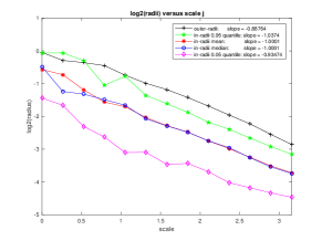
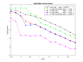
We observe that the vast majority of $C_{j,k}$’s constructed above satisfy Assumption (A1-A5) in our numerical experiments. In Fig. 13, we will show that (A5) is satisfied when we experiment on volume measures on the $3$-dim S and Z manifold. Here we sample $10^{5}$ training data, perform multiscale tree decomposition as stated above, and compute $\theta_{3}^{j,k},\theta_{4}^{j,k}$ at every $C_{j,k}$. In Fig. 13, we display the mean of $\{\theta_{3}^{j,k}\}_{k\in\mathcal{K}_{j}}$ or $\{\theta_{4}^{j,k}\}_{k\in\mathcal{K}_{j}}$ versus scale $j$, with a vertical error bar representing the standard deviation of $\{\theta_{3}^{j,k}\}_{k\in\mathcal{K}_{j}}$ or $\{\theta_{4}^{j,k}\}_{k\in\mathcal{K}_{j}}$ at each scale. We observe that $\theta_{3}=\min_{j,k}\theta_{3}^{j,k}\geq 0.05$ at all scales and $\theta_{4}=\max_{j,k}\theta_{4}^{j,k}\leq 1/2$ except at very coarse scales, which demonstrates Assumption (A5) is satisfied here. Indeed $\theta_{4}$ is not only bounded, but also decreases from coarse scales to fine scales.

(a) $\{\theta_{3}^{j,k}\}_{k\in\mathcal{K}_{j}}$ versus $j$ of the $3$-dim S manifold

(b) $\{\theta_{4}^{j,k}\}_{k\in\mathcal{K}_{j}}$ versus $j$ of the $3$-dim S manifold

(c) $\{\theta_{3}^{j,k}\}_{k\in\mathcal{K}_{j}}$ versus $j$ of the $3$-dim Z manifold

(d) $\{\theta_{4}^{j,k}\}_{k\in\mathcal{K}_{j}}$ versus $j$ of the $3$-dim Z manifold

Figure 13: The mean of $\{\theta_{3}^{j,k}\}_{k\in\mathcal{K}_{j}}$ or $\{\theta_{4}^{j,k}\}_{k\in\mathcal{K}_{j}}$ versus scale $j$, with a vertical error bar representing the standard deviation of $\{\theta_{3}^{j,k}\}_{k\in\mathcal{K}_{j}}$ or $\{\theta_{4}^{j,k}\}_{k\in\mathcal{K}_{j}}$ at each scale.

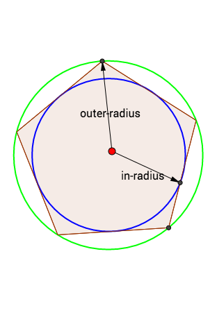
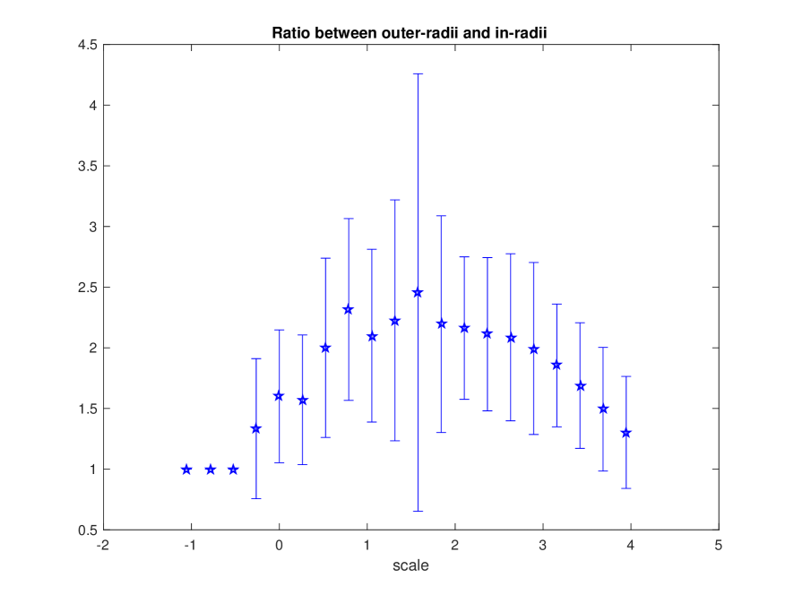
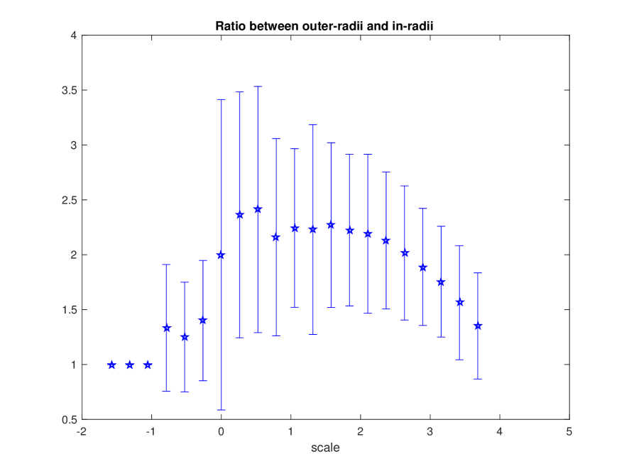
We observe that, every $C_{j,k}$ constructed above is contained in a ball of radius $\theta_{2}2^{-j}$ and contains a ball of radius $\theta_{0}2^{-j}$, with $\theta_{2}/\theta_{0}\in[1,2]$ for the majority of $C_{j,k}$’s. In Fig. 14, we take the volume measures on the $3$-dim S and Z manifold, and plot $\log_{2}$ of the outer-radius and the statistics a lower bound for the in-radius versus the scale of cover tree. Notice that the in-radius is a fraction of the outer-radius at all scales, and $\log_{2}\theta_{2}-\log_{2}\theta_{0}\leq 1$ for the majority of cells.

Figure 14: From left to right: the in-radius and outer-radius of a pentagon; $\log_{2}$ of the outer-radius and the statistics of the in-radius versus the scale of cover tree for the $3$-dim S manifold, and then the same plot for the $3$-dim Z manifold; ratio between outer-radii and in-radii, for the $3$-dim S manifold top) and the $3$-dim Z manifold (bottom).

A.4 $\mathcal{A}_{s}^{\infty}\subset\mathcal{B}_{s}$

Proof [proof of Lemma 6] Assume $\rho(C_{j,k})\asymp 2^{-jd}$. According to Definition 2, $\rho\in\mathcal{A}_{s}^{\infty}$ if $\|(X-\mathcal{P}_{j,k}X)\mathbf{1}_{j,k}\|\leq|\rho|_{\mathcal{A}_{s}^{\infty}}2^{-js}\sqrt{\rho(C_{j,k})},\ \forall k\in\mathcal{K}_{j},j\geq j_{\rm min}$, which implies $\Delta_{j,k}\leq 2|\rho|_{\mathcal{A}_{s}^{\infty}}2^{-js}\sqrt{\rho(C_{j,k})}\lesssim|\rho|_{\mathcal{A}_{s}^{\infty}}2^{-j(s+\frac{d}{2})}$.

Let $\eta>0$ and $\mathcal{T}_{(\rho,\eta)}$ be the smallest proper subtree of $\mathcal{T}$ that contains all $C_{j,k}$ for which $\Delta_{j,k}\ \geq 2^{-j}\eta$. All the nodes satisfying $\Delta_{j,k}\geq 2^{-j}\eta$ will satisfy $|\rho|_{\mathcal{A}_{s}^{\infty}}2^{-j(s+\frac{d}{2})}\gtrsim 2^{-j}\eta$ which implies $2^{-j}\gtrsim({\eta}/{|\rho|_{\mathcal{A}_{s}^{\infty}}})^{\frac{2}{2s+d-2}}$. Therefore, the truncated tree $\mathcal{T}_{(\rho,\eta)}$ is contained in $\mathcal{T}_{j^{*}}=\cup_{j\leq j^{*}}\Lambda_{j}$ with $2^{-j^{*}}\asymp(\eta/|\rho|_{\mathcal{A}_{s}^{\infty}})^{\frac{2}{2s+d-2}}$, so the entropy of $\mathcal{T}_{(\rho,\eta)}$ is upper bounded by the entropy of $\mathcal{T}_{j^{*}}$, which is $\sum_{j\leq j^{*}}2^{-2j}\#\Lambda_{j}\asymp 2^{j^{*}(d-2)}\asymp(\eta/|\rho|_{\mathcal{A}_{s}^{\infty}})^{-\frac{2(d-2)}{2s+d-2}}$. Then $\rho\in\mathcal{B}_{s}$ and $|\rho|_{\mathcal{B}_{s}}\lesssim|\rho|_{\mathcal{A}_{s}^{\infty}}$ according to Definition 5.  

B S manifold and Z manifold

We consider volume measures on the $d$ dimensional S manifold and Z manifold whose $x_{1}$ and $x_{2}$ coordinates are on the S curve and Z curve in Figure 5 (a) and $x_{i},i=3,\ldots,d+1$ are uniformly distributed in $[0,1]$.

B.1 S manifold

Since S manifold is smooth and has a bounded curvature, the volume measure on the S manifold is in $\mathcal{A}_{2}^{\infty}$. Therefore, the volume measure on the S manifold is in $\mathcal{A}_{2}$ and $\mathcal{B}_{2}$ when $d\geq 3$.

B.2 Z manifold

B.2.1 The volume on the Z manifold is in $\mathcal{A}_{1.5}$

The uniform distribution on the $d$ dimensional Z manifold is in $\mathcal{A}_{1}$ at two corners and satisfies $\|(X-\mathcal{P}_{j,k}X)\mathbf{1}_{j,k}\|=0$ when $C_{j,k}$ is away from the corners. There exists $A_{0}>0$ such that $\|(X-\mathcal{P}_{j,k}X)\mathbf{1}_{j,k}\|\leq A_{0}2^{-j}\sqrt{\rho(C_{j,k})}$ when $C_{j,k}$ intersects with the corners. At scale $j$, there are about $2^{jd}$ cells away from the corners and there are about $2^{j(d-1)}$ cells which intersect with the corners. As a result,

$$\|X-\mathcal{P}_{j}X\| \leq\mathcal{O}\left(\sqrt{2^{jd}\cdot 0\cdot 2^{-jd}+2^{j(d-1)}\cdot 2^{-2j}\cdot 2^{-jd}}\right)=\mathcal{O}(2^{-1.5j}),$$

so the volume measure on Z manifold is in $\mathcal{A}_{1.5}$.

B.2.2 Model class $\mathcal{B}_{s}$

Assume $\rho(C_{j,k})\asymp 2^{-jd}$. We compute the regularity parameter $s$ in the $\mathcal{B}_{s}$ model class when $d\geq 3$. It is easy to see that $\Delta_{j,k}=0$ when $C_{j,k}$ is away from the corners and $\Delta_{j,k}\leq 2A_{0}2^{-j}\sqrt{\rho(C_{j,k})}\lesssim 2^{-j(\frac{d}{2}+1)}$ when $C_{j,k}$ intersects with the corners. Given any fixed threshold $\eta>0$, in the truncated tree $\mathcal{T}_{(\rho,\eta)}$, the parent of the leaves intersecting with the corners satisfy $2^{-j(\frac{d}{2}+1)}\gtrsim 2^{-j}\eta$. In other words, at the corners the tree is truncated at a scale coarser than $j^{*}$ such that $2^{-j^{*}}=\mathcal{O}(\eta^{\frac{2}{d}})$. Since $\Delta_{j,k}=0$ when $C_{j,k}$ is away from the corners, the entropy of $\mathcal{T}_{(\rho,\eta)}$ is dominated by the nodes intersecting with the corners whose cardinality is $2^{j(d-1)}$ at scale $j$. Therefore

$$\text{Entropy of }\mathcal{T}_{(\rho,\eta)}\lesssim\sum_{j\leq j^{*}}2^{-2j}2^{j(d-1)}=\mathcal{O}\left(\eta^{-\frac{2(d-3)}{d}}\right),$$

which implies that $p\leq\frac{2(d-3)}{d}$ and $s\geq\frac{3(d-2)}{2(d-3)}>1.5$.

Then we study the relation between the error $\|X-\mathcal{P}_{\Lambda_{(\rho,\eta)}}X\|$ and the partition size $\#\Lambda_{(\rho,\eta)}$, which is numerically verified in Figure 4. Since all the nodes in $\mathcal{T}_{(\rho,\eta)}$ that intersect with corners are at a scale coarser than $j^{*}$, $\#\Lambda_{(\rho,\eta)}\approx 2^{j^{*}(d-1)}\asymp\eta^{-\frac{2(d-1)}{d}}$. Therefore, $\eta\lesssim[\#\Lambda_{(\rho,\eta)}]^{-\frac{d}{2(d-1)}}$ and

$$\|X-\mathcal{P}_{\Lambda_{(\rho,\eta)}}X\|\lesssim\eta^{\frac{2-p}{2}}=\eta^{\frac{2s}{2s+d-2}}\lesssim[\#\Lambda_{(\rho,\eta)}]^{-\frac{2sd}{2(d-1)(2s+d-2)}}=[\#\Lambda_{(\rho,\eta)}]^{-\frac{3}{2(d-1)}}.$$

C Proofs of Lemma 14 and Proposition 15

C.1 Concentration inequalities

We first recall a Bernstein inequality from Tropp (2014) which is an exponential inequality to estimate the spectral norm of a sum independent random Hermitian matrices of size $D\times D$. It features the dependence on an intrinsic dimension parameter which is usually much smaller than the ambient dimension $D$. For a positive-semidefinite matrix $A$, the intrinsic dimension is the quantity

$${\rm intdim}(A)=\frac{{{\rm trace}}(A)}{\|A\|}.$$

Proposition 27 (Theorem 7.3.1 in Tropp (2014))

Let $\xi_{1},\ldots,\xi_{n}$ be $D\times D$ independent random Hermitian matrices that satisfy

$$\mathbb{E}\xi_{i}=0\ \text{and}\ \|\xi_{i}\|\leq R,\ i=1,\ldots,n.$$

Form the mean $\xi=\frac{1}{n}\sum_{i=1}^{n}\xi_{i}$. Suppose $\mathbb{E}(\xi^{2})\preceq\Phi.$ Introduce the intrinsic dimension parameter $d_{\rm in}={\rm intdim}(\Phi).$ Then, for $nt\geq n\|\Phi\|^{1/2}+R/3$,

$$\mathbb{P}\{\|\xi\|\geq t\}\leq 4d_{\rm in}e^{-\frac{nt^{2}/2}{n\|\Phi\|+Rt/3}}.$$

We use the above inequalities to estimate the deviation of the empirical mean from the mean and the deviation of the empirical covariance matrix from the covariance matrix when the data $\mathcal{X}_{j,k}=\{x_{1},\ldots,x_{n}\}$ (with a slight abuse of notations) are i.i.d. samples from the distribution $\rho|_{C_{j,k}}$.

Lemma 28

Suppose $x_{1},\ldots,x_{n}$ are i.i.d. samples from $\rho|_{C_{j,k}}$. Let

$$c_{j,k}=\int_{C_{j,k}}xd\rho|_{C_{j,k}} \widehat{c}_{j,k}:=\frac{1}{n}\sum_{i=1}^{n}x_{i}$$ ,

$$\Sigma_{j,k}=\int_{C_{j,k}}(x-c_{j,k})(x-c_{j,k})^{T}d\rho|_{C_{j,k}} \widehat{\Sigma}_{j,k}:=\frac{1}{n}\sum_{i=1}^{n}(x_{i}-\widehat{c}_{j,k})(x_{i}-\widehat{c}_{j,k})^{T}$$ ,

Then

$$\mathbb{P}\{\|\widehat{c}_{j,k}-c_{j,k}\|\geq t\} \leq 8e^{-\frac{3nt^{2}}{6\theta_{2}^{2}2^{-2j}+2\theta_{2}2^{-j}t}}\,,$$ (35)

$$\mathbb{P}\{\|\widehat{\Sigma}_{j,k}-\Sigma_{j,k}\|\geq t\} \leq \left(\frac{4\theta_{2}^{2}}{\theta_{3}}d+8\right)e^{-\frac{3nt^{2}}{24\theta_{2}^{4}2^{-4j}+8\theta_{2}^{2}2^{-2j}t}}\,.$$ (36)

Proof We start by proving (35). We will apply Bernstein inequality with $\xi_{i}=x_{i}-c_{j,k}\in\mathbb{R}^{D}$. Clearly $\mathbb{E}\xi_{i}=0$, and $\|\xi_{i}\|\leq{\theta_{2}2^{-j}}$ due to Assumption (A4). We form the mean $\xi=\frac{1}{n}\sum_{i=1}^{n}\xi_{i}=\widehat{c}_{j,k}-c_{j,k}$ and compute the variance

$$\sigma^{2} =n^{2}\|\mathbb{E}\xi^{T}\xi\|=\left\|\mathbb{E}\left(\sum_{i=1}^{n}{x_{i}-c_{j,k}}\right)^{T}\left(\sum_{i=1}^{n}{x_{i}-c_{j,k}}\right)\right\|=\left\|\sum_{i=1}^{n}{\mathbb{E}(x_{i}-c_{j,k})^{T}(x_{i}-c_{j,k})}\right\|\leq n{\theta_{2}^{2}2^{-2j}}.$$

Then for $nt\geq\sigma+\theta_{2}2^{-j}/3$,

$$\mathbb{P}\{\|\widehat{c}_{j,k}-c_{j,k}\|\geq t\}\leq 8e^{-\frac{n^{2}t^{2}/3}{\sigma^{2}+\theta_{2}2^{-j}nt/3}}\leq 8e^{-\frac{3nt^{2}}{6\theta_{2}^{2}2^{-2j}+2\theta_{2}2^{-j}t}}.$$

We now prove (36). Define the intermediate matrix $\bar{\Sigma}_{j,k}=\frac{1}{n}\sum_{i=1}^{n}(x_{i}-c_{j,k})(x_{i}-c_{j,k})^{T}.$ Since $\widehat{\Sigma}_{j,k}-\Sigma_{j,k}=\bar{\Sigma}_{j,k}-\Sigma_{j,k}-(\widehat{c}_{j,k}-c_{j,k})(\widehat{c}_{j,k}-c_{j,k})^{T},$ we have

$$\|\widehat{\Sigma}_{j,k}-\Sigma_{j,k}\|\leq\|\bar{\Sigma}_{j,k}-\Sigma_{j,k}\|+\|\widehat{c}_{j,k}-c_{j,k}\|^{2}\leq\|\bar{\Sigma}_{j,k}-\Sigma_{j,k}\|+\theta_{2}2^{-j}\|\widehat{c}_{j,k}-c_{j,k}\|.$$

A sufficient condition for $\|\widehat{\Sigma}_{j,k}-\Sigma_{j,k}\|<t$ is $\|\bar{\Sigma}_{j,k}-\Sigma_{j,k}\|<t/2$ and $\|\widehat{c}_{j,k}-c_{j,k}\|<2^{j}t/(2\theta_{2})$. We apply Proposition 27 to estimate $\mathbb{P}\{\|\bar{\Sigma}_{j,k}-\Sigma_{j,k}\|\geq t/2\}$: let $\xi_{i}=(x_{i}-c_{j,k})(x_{i}-c_{j,k})^{T}-\Sigma_{j,k}\in\mathbb{R}^{D\times D}.$ One can verify that $\mathbb{E}\xi_{i}=0\ \text{and}\ \|\xi_{i}\|\leq{2\theta_{2}^{2}2^{-2j}}.$ We form the mean $\xi=\frac{1}{n}\sum_{i=1}^{n}\xi_{i}=\bar{\Sigma}_{j,k}-\Sigma_{j,k}$, and then

$$\mathbb{E}\xi^{2} =\mathbb{E}\left(\frac{1}{n^{2}}\sum_{i=1}^{n}\xi_{i}\sum_{i=1}^{n}\xi_{i}\right)=\frac{1}{n^{2}}\sum_{i=1}^{n}\mathbb{E}\xi_{i}^{2}\preceq\frac{1}{n^{2}}\sum_{i=1}^{n}{\theta_{2}^{2}2^{-2j}}\Sigma_{j,k}\preceq\frac{\theta_{2}^{2}2^{-2j}}{n}\Sigma_{j,k},$$

which satisfies $\left\|\frac{\theta_{2}^{2}2^{-2j}}{n}\Sigma_{j,k}\right\|\leq{\theta_{2}^{4}2^{-4j}}/{n}.$ Meanwhile

$$d_{\rm in}={\rm intdim}(\Sigma_{j,k})=\frac{{\rm trace}(\Sigma_{j,k})}{\|\Sigma_{j,k}\|}\leq\frac{\theta_{2}^{2}2^{-2j}}{\theta_{3}2^{-2j}/d}=\frac{\theta_{2}^{2}}{\theta_{3}}d.$$

Then, Proposition 27 implies

$$\mathbb{P}\{\|\bar{\Sigma}_{j,k}-\Sigma_{j,k}\|\geq t/2\}\leq\frac{4\theta_{2}^{2}}{\theta_{3}}de^{\frac{-nt^{2}/8}{\theta_{2}^{4}2^{-4j}+\frac{\theta_{2}^{2}2^{-2j}t}{3}}}=\frac{4\theta_{2}^{2}}{\theta_{3}}de^{\frac{-3nt^{2}}{24\theta_{2}^{4}2^{-4j}+8\theta_{2}^{2}2^{-2j}t}}\,.$$

Combining with (35), we obtain

$$\mathbb{P}\{\|\widehat{\Sigma}_{j,k}-\Sigma_{j,k}\|\geq t\} \leq\mathbb{P}\{\|\bar{\Sigma}_{j,k}-\Sigma_{j,k}\|\geq t/2\}+\mathbb{P}\left\{\|\widehat{c}_{j,k}-c_{j,k}\|\geq\frac{2^{j}t}{2\theta_{2}}\right\}$$

$$\leq\left(\frac{4\theta_{2}^{2}}{\theta_{3}}d+8\right)e^{-\frac{3nt^{2}}{24\theta_{2}^{4}2^{-4j}+8\theta_{2}^{2}2^{-2j}t}}\,.$$

 

In Lemma 28 data are assumed to be i.i.d. samples from the conditional distribution $\rho|_{C_{j,k}}$. Given $\mathcal{X}_{n}=\{x_{1},\ldots,x_{n}\}$ which contains i.i.d. samples from $\rho$, we will show that the empirical measure $\widehat{\rho}(C_{j,k})=\widehat{n}_{j,k}/n$ is close to $\rho(C_{j,k})$ with high probability.

Lemma 29

Suppose $x_{1},\ldots,x_{n}$ are i.i.d. samples from $\rho$. Let $\rho(C_{j,k})=\int_{C_{j,k}}1d\rho$ and $\widehat{\rho}(C_{j,k})=\widehat{n}_{j,k}/n$ where $\widehat{n}_{j,k}$ is the number of points in $C_{j,k}$. Then

$$\mathbb{P}\{\left|\widehat{\rho}(C_{j,k})-\rho(C_{j,k})\right|\geq t\}\leq 2e^{-\frac{3nt^{2}}{6\rho(C_{j,k})+2t}}$$ (37)

for all $t\geq 0$. Setting $t=\frac{1}{2}\rho(C_{j,k})$ gives rise to

$$\mathbb{P}\left\{|\widehat{\rho}(C_{j,k})-\rho(C_{j,k})|\geq\frac{1}{2}\rho(C_{j,k})\right\}\leq 2e^{-\frac{3}{28}n\rho(C_{j,k})}.$$ (38)

Combining Lemma 28 and Lemma 29 gives rise to probability bounds on $\|\widehat{c}_{j,k}-c_{j,k}\|$ and $\|\widehat{\Sigma}_{j,k}-\Sigma_{j,k}\|$ where $c_{j,k}$, $\widehat{c}_{j,k}$, $\Sigma_{j,k}$ and $\widehat{\Sigma}_{j,k}$ are the conditional mean, empirical conditional mean, conditional covariance matrix and empirical conditional covariance matrix on $C_{j,k}$, respectively.

Lemma 30

Suppose $x_{1},\ldots,x_{n}$ are i.i.d. samples from $\rho$. Define $c_{j,k},\Sigma_{j,k}$ and $\widehat{c}_{j,k},\widehat{\Sigma}_{j,k}$ as Table 1. Then given any $t>0$,

$$\mathbb{P}\left\{\|\widehat{c}_{j,k}-c_{j,k}\|\geq t\right\} \leq 2e^{-\frac{3}{28}n\rho(C_{j,k})}+8e^{-\frac{3n\rho(C_{j,k})t^{2}}{12\theta_{2}^{2}2^{-2j}+4\theta_{2}2^{-j}t}}\,,$$ (39)

$$\mathbb{P}\left\{\|\widehat{\Sigma}_{j,k}-\Sigma_{j,k}\|\geq t\right\} \leq 2e^{-\frac{3}{28}n\rho(C_{j,k})}+\left(\frac{4\theta_{2}^{2}}{\theta_{3}}d+8\right)e^{-\frac{3n\rho(C_{j,k})t^{2}}{96\theta_{2}^{4}2^{-4j}+16\theta_{2}^{2}2^{-2j}t}}\,.$$ (40)

Proof The number of samples on $C_{j,k}$ is $\widehat{n}_{j,k}=\sum_{i=1}^{n}\mathbf{1}_{j,k}(x_{i})$. Clearly $\mathbb{E}[\widehat{n}_{j,k}]=n\rho(C_{j,k})$. Let $\mathcal{I}\subset\{1,\ldots,n\}$ and $|\mathcal{I}|=s$. Conditionally on the event $A_{\mathcal{I}}:=\{x_{i}\in C_{j,k}\text{ for }i\in\mathcal{I}\text{ and }x_{i}\notin C_{j,k}\text{ for }i\notin\mathcal{I}\}$, the random variables $\{x_{i},i\in\mathcal{I}\}$ are i.i.d. samples from $\rho|_{C_{j,k}}$. According to Lemma 29,

$$\mathbb{P}\{\|\widehat{c}_{j,k}-c_{j,k}\|\geq t\ |\ \widehat{n}_{j,k}=s\}=\sum_{\begin{subarray}{c}\mathcal{I}\subset\{1,\ldots,n\}\\ |\mathcal{I}|=s\end{subarray}}\mathbb{P}\{\|\widehat{c}_{j,k}-c_{j,k}\|\geq t\ |\ A_{\mathcal{I}}\}\frac{1}{\binom{n}{s}}$$

$$=\mathbb{P}\{\|\widehat{c}_{j,k}-c_{j,k}\|\geq t\ |\ A_{\{1,\ldots,s\}}\}\leq 8e^{-\frac{3st^{2}}{6\theta_{2}^{2}2^{-2j}+2\theta_{2}2^{-j}t}},$$

and

$$\mathbb{P}\{\|\widehat{\Sigma}_{j,k}-\Sigma_{j,k}\|\geq t\ |\ \widehat{n}_{j,k}=s\}\leq\left(\frac{4\theta_{2}^{2}}{\theta_{3}}d+8\right)e^{-\frac{3st^{2}}{24\theta_{2}^{4}2^{-4j}+8\theta_{2}^{2}2^{-2j}t}}\,.$$

Furthermore $|\widehat{\rho}(C_{j,k})-\rho(C_{j,k})|\leq\frac{1}{2}\rho(C_{j,k})$ yields $\widehat{n}_{j,k}\geq\frac{1}{2}n\rho(C_{j,k})$ and then

$$\mathbb{P}\left\{\|\widehat{c}_{j,k}-c_{j,k}\|\geq t\ \Big{|}\ |\widehat{\rho}(C_{j,k})-\rho(C_{j,k})|\leq\frac{1}{2}\rho(C_{j,k})\right\}\leq 8e^{-\frac{3n\rho(C_{j,k})t^{2}}{12\theta_{2}^{2}2^{-2j}+4\theta_{2}2^{-j}t}}\,,$$ (41)

$$\mathbb{P}\left\{\|\widehat{\Sigma}_{j,k}-\Sigma_{j,k}\|\geq t\ \Big{|}\ |\widehat{\rho}(C_{j,k})-\rho(C_{j,k})|\leq\frac{1}{2}\rho(C_{j,k})\right\}\leq\left(\frac{4\theta_{2}^{2}}{\theta_{3}}d+8\right)e^{-\frac{3n\rho(C_{j,k})t^{2}}{48\theta_{2}^{4}2^{-4j}+16\theta_{2}^{2}2^{-2j}t}}\,.$$ (42)

Eq. (41) (42) along with Lemma 29 gives rise to

$$\mathbb{P}\left\{\|\widehat{c}_{j,k}-c_{j,k}\|\geq t\right\}\leq 2e^{-\frac{3}{28}n\rho(C_{j,k})}+8e^{-\frac{3n\rho(C_{j,k})t^{2}}{12\theta_{2}^{2}2^{-2j}+4\theta_{2}2^{-j}t}}\,,$$

$$\mathbb{P}\left\{\|\widehat{\Sigma}_{j,k}-\Sigma_{j,k}\|\geq t\right\}\leq 2e^{-\frac{3}{28}n\rho(C_{j,k})}+\left(\frac{4\theta_{2}^{2}}{\theta_{3}}d+8\right)e^{-\frac{3n\rho(C_{j,k})t^{2}}{48\theta_{2}^{4}2^{-4j}+16\theta_{2}^{2}2^{-2j}t}}\,.$$

 

Given $\|\widehat{\Sigma}_{j,k}-\Sigma_{j,k}\|$, we can estimate the angle between the eigenspace of $\widehat{\Sigma}_{j,k}$ and $\Sigma_{j,k}$ with the following proposition.

Proposition 31 (Davis and Kahan (1970) or Theorem 3 in Zwald and Blanchard (2006))

Let $\delta_{d}(\Sigma_{j,k})=\frac{1}{2}(\lambda_{d}^{j,k}-\lambda_{d+1}^{j,k})$. If $\|\widehat{\Sigma}_{j,k}-\Sigma_{j,k}\|\leq\frac{1}{2}{\delta_{d}(\Sigma_{j,k})}$, then

$$\left\|{\rm Proj}_{V_{j,k}}-{\rm Proj}_{\widehat{V}_{j,k}}\right\|\leq\frac{\|\widehat{\Sigma}_{j,k}-\Sigma_{j,k}\|}{\delta_{d}(\Sigma_{j,k})}.$$

According to Assumption (A4) and (A5), $\delta_{d}(\Sigma_{j,k})\geq\theta_{3}2^{-2j}/(4d)$. An application of Proposition 31 yields

$$\mathbb{P}\left\{\|{\rm Proj}_{V_{j,k}}-{\rm Proj}_{\widehat{V}_{j,k}}\right\|\geq t\}\leq\mathbb{P}\left\{\|\widehat{\Sigma}_{j,k}-\Sigma_{j,k}\|\geq\frac{\theta_{3}(1-\theta_{4})t}{2d2^{2j}}\right\}$$

$$\leq 2e^{-\frac{3}{28}n\rho(C_{j,k})}+\left(\frac{4\theta_{2}^{2}}{\theta_{3}}d+8\right)e^{-\frac{3\theta_{3}^{2}(1-\theta_{4})^{2}n\rho(C_{j,k})t^{2}}{384\theta_{2}^{4}d^{2}+32\theta_{2}^{2}\theta_{3}(1-\theta_{4})dt}}\,.$$ (43)

Proof [Proof of Lemma 14] Since

$$\|\mathcal{P}_{\Lambda}X-\widehat{\mathcal{P}}_{\Lambda}X\|^{2}=\sum_{C_{j,k}\in\Lambda}\int_{C_{j,k}}\|\mathcal{P}_{j,k}x-\widehat{\mathcal{P}}_{j,k}x\|^{2}d\rho=\sum_{j}\sum_{k:C_{j,k}\in\Lambda}\int_{C_{j,k}}\|\mathcal{P}_{j,k}x-\widehat{\mathcal{P}}_{j,k}x\|^{2}d\rho,$$

we obtain the estimate

$$\mathbb{P}\left\{\|\mathcal{P}_{\Lambda}X-\widehat{\mathcal{P}}_{\Lambda}X\|\geq\eta\right\}\leq\sum_{j}\mathbb{P}\left\{\sum_{k:C_{j,k}\in\Lambda}\int_{C_{j,k}}\|\mathcal{P}_{j,k}x-\widehat{\mathcal{P}}_{j,k}x\|^{2}d\rho\geq\frac{2^{-2j}\#_{j}\Lambda\eta^{2}}{\sum_{j\geq j_{\rm min}}2^{-2j}\#_{j}\Lambda}\right\}.$$ (44)

Next we prove that, for any fixed scale $j$,

$$\mathbb{P}\left\{\sum_{k:C_{j,k}\in\Lambda}\int_{C_{j,k}}\|\mathcal{P}_{j,k}x-\widehat{\mathcal{P}}_{j,k}x\|^{2}d\rho\geq t^{2}\right\}\leq\alpha\#_{j}\Lambda e^{-\frac{\beta 2^{2j}nt^{2}}{\#_{j}\Lambda}}.$$ (45)

Then Lemma 14 is proved by setting $t^{2}=2^{-2j}\#_{j}\Lambda\eta^{2}/(\sum_{j\geq 0}2^{-2j}\#_{j}\Lambda)$.

The proof of (45) starts with the following calculation:

$$\sum_{k:C_{j,k}\in\Lambda}\int_{C_{j,k}}\|\mathcal{P}_{j,k}x-\widehat{\mathcal{P}}_{j,k}x\|^{2}d\rho$$

$$=\sum_{k:C_{j,k}\in\Lambda}\int_{C_{j,k}}\|c_{j,k}+{\rm Proj}_{V_{j,k}}(x-c_{j,k})-\widehat{c}_{j,k}-{\rm Proj}_{\widehat{V}_{j,k}}(x-\widehat{c}_{j,k})\|^{2}d\rho$$

$$\leq\sum_{k:C_{j,k}\in\Lambda}\int_{C_{j,k}}\|(\mathbb{I}-{\rm Proj}_{\widehat{V}_{j,k}})(c_{j,k}-\widehat{c}_{j,k})+({\rm Proj}_{V_{j,k}}-{\rm Proj}_{\widehat{V}_{j,k}})(x-c_{j,k})\|^{2}d\rho$$

$$\leq 2\sum_{k:C_{j,k}\in\Lambda}\int_{C_{j,k}}\left[\|c_{j,k}-\widehat{c}_{j,k}\|^{2}+\|({\rm Proj}_{V_{j,k}}-{\rm Proj}_{\widehat{V}_{j,k}})(x-c_{j,k})\|^{2}\right]d\rho$$

$$\leq 2\sum_{k:C_{j,k}\in\Lambda}\int_{C_{j,k}}\left[\|c_{j,k}-\widehat{c}_{j,k}\|^{2}+\theta_{2}^{2}2^{-2j}\|{\rm Proj}_{V_{j,k}}-{\rm Proj}_{\widehat{V}_{j,k}}\|^{2}\right]d\rho$$

For any fixed $j$ and given $t>0$, we divide $\Lambda$ into light cells $\Lambda_{j,t}^{-}$ and heavy cells $\Lambda_{j,t}^{+}$, where

$$\Lambda^{-}_{j,t}:=\left\{C_{j,k}\in\Lambda:\rho(C_{j,k})\leq\frac{t^{2}}{20\theta_{2}^{2}2^{-2j}\#_{j}\Lambda}\right\}\ \text{and}\ \Lambda^{+}_{j,t}:=\Lambda\setminus\Lambda^{-}_{j,t}\,.$$

Since $\int_{C_{j,k}}\left[\|c_{j,k}-\widehat{c}_{j,k}\|^{2}+\theta_{2}^{2}2^{-2j}\|{\rm Proj}_{V_{j,k}}-{\rm Proj}_{\widehat{V}_{j,k}}\|^{2}\right]d\rho\leq 5\theta_{2}^{2}2^{-2j}\rho(C_{j,k})$, for light sets we have

$$2\sum_{k:C_{j,k}\in\Lambda_{j,t}^{-}}\int_{C_{j,k}}\left[\|c_{j,k}-\widehat{c}_{j,k}\|^{2}+\theta_{2}^{2}2^{-2j}\|{\rm Proj}_{V_{j,k}}-{\rm Proj}_{\widehat{V}_{j,k}}\|^{2}\right]d\rho\leq\frac{t^{2}}{2}.$$ (46)

Next we consider $C_{j,k}\in\Lambda_{j,t}^{+}$. We have

$$\mathbb{P}\left\{\|\widehat{c}_{j,k}-c_{j,k}\|\geq\frac{t}{\sqrt{8\#_{j}\Lambda\rho(C_{j,k})}}\right\}$$

$$\leq 2\exp\left(-\frac{3}{28}n\rho(C_{j,k})\right)+8e^{-\frac{3n\rho(C_{j,k})\frac{t^{2}}{8\#_{j}\Lambda\rho(C_{j,k})}}{12\theta_{2}^{2}2^{-2j}+4\theta_{2}2^{-j}\frac{t}{\sqrt{8\#_{j}\Lambda\rho(C_{j,k})}}}}\leq C_{1}e^{-C_{2}\frac{2^{2j}nt^{2}}{\#_{j}\Lambda}},$$ (47)

and

$$\mathbb{P}\left\{\|{\rm Proj}_{V_{j,k}}-{\rm Proj}_{\widehat{V}_{j,k}}\|\geq\frac{2^{j}t}{\theta_{2}\sqrt{8\#_{j}\Lambda\rho(C_{j,k})}}\right\}$$

$$\leq 2e^{-\frac{3}{28}n\rho(C_{j,k})}+\left(\frac{4\theta_{2}^{2}}{\theta_{3}}d+8\right)e^{-\frac{3\theta_{3}^{2}(1-\theta_{4})^{2}n\rho(C_{j,k})\frac{2^{2j}t^{2}}{8\theta_{2}^{2}\#_{j}\Lambda\rho(C_{j,k})}}{384\theta_{2}^{4}d^{2}+32\theta_{2}^{2}\theta_{3}(1-\theta_{4})d\frac{2^{j}t}{\theta_{2}\sqrt{8\#_{j}\Lambda\rho(C_{j,k})}}}}\leq C_{3}de^{-C_{4}\frac{2^{2j}nt^{2}}{d^{2}\#_{j}\Lambda}}$$ (48)

where positive constants $C_{1},C_{2},C_{3},C_{4}$ depend on $\theta_{2}$ and $\theta_{3}$. Combining (46), (47) and (48) gives rise to (45) with $\alpha=\max(C_{1},C_{3})$ and $\beta=\min(C_{2},C_{4}).$

 

Proof [Proof of Proposition 15] The bound (18) follows directly from Lemma 14 applied to $\Lambda=\Lambda_{j}$; (19) follows from (18) by integrating the probability over $\eta$:

$$\mathbb{E}\|\mathcal{P}_{j}X-\widehat{\mathcal{P}}_{j}X\|^{2}=\int_{0}^{+\infty}\eta\mathbb{P}\left\{\|\mathcal{P}_{j}X-\widehat{\mathcal{P}}_{j}X\|\geq\eta\right\}d\eta$$

$$\leq\int_{0}^{+\infty}\eta\min\left\{1,\alpha d\#\Lambda_{j}e^{-\frac{\beta 2^{2j}n\eta^{2}}{d^{2}\#\Lambda_{j}}}\right\}d\eta=\int_{0}^{\eta_{0}}\eta d\eta+\int_{\eta_{0}}^{+\infty}\alpha d\eta\#\Lambda_{j}e^{-\frac{\beta 2^{2j}n\eta^{2}}{d^{2}\#\Lambda_{j}}}d\eta$$

where $\alpha d\#\Lambda_{j}e^{-\frac{\beta 2^{2j}n\eta_{0}^{2}}{d^{2}\#\Lambda_{j}}}=1$. Then

$$\mathbb{E}\|\mathcal{P}_{j}X-\widehat{\mathcal{P}}_{j}X\|^{2}=\frac{1}{2}\eta_{0}^{2}+\frac{\alpha}{2\beta}\cdot\frac{\#\Lambda_{j}^{2}}{2^{2j}n}e^{-\beta\frac{2^{2j}n\eta_{0}^{2}}{\#\Lambda_{j}}}\leq\frac{d^{2}\#\Lambda_{j}\log[\alpha d\#\Lambda_{j}]}{\beta 2^{2j}n}.$$

 

D Proof of Eq. (9), Lemma 16, 18, 19, 20

D.1 Proof of Eq. (9)

Let $\Lambda^{+0}_{(\rho,\eta)}=\Lambda_{(\rho,\eta)}$ and $\Lambda^{+n}_{(\rho,\eta)}$ be the partition consisting of the children of $\Lambda^{+(n-1)}_{(\rho,\eta)}$ for $n=1,2,\ldots$. Then

$$\|X-\mathcal{P}_{\Lambda_{(\rho,\eta)}}X\| =\|\sum_{\ell=0}^{n-1}(\mathcal{P}_{\Lambda^{+\ell}_{(\rho,\eta)}}X-\mathcal{P}_{\Lambda^{+(\ell+1)}_{(\rho,\eta)}}X)+\mathcal{P}_{\Lambda^{+n}(\rho,\eta)}X-X\|$$

$$=\|\sum_{\ell=0}^{\infty}(\mathcal{P}_{\Lambda^{+\ell}_{(\rho,\eta)}}X-\mathcal{P}_{\Lambda^{+(\ell+1)}_{(\rho,\eta)}}X)+\lim_{n\rightarrow\infty}\mathcal{P}_{\Lambda^{+n}_{(\rho,\eta)}}X-X\|$$

$$\leq\|\sum_{C_{j,k}\notin\mathcal{T}_{(\rho,\eta)}}\mathcal{Q}_{j,k}X\|+\|\lim_{n\rightarrow\infty}\mathcal{P}_{\Lambda^{+n}_{(\rho,\eta)}}X-X\|.$$

We have $\|\lim_{n\rightarrow\infty}\mathcal{P}_{\Lambda^{+n}_{(\rho,\eta)}}X-X\|=0$ due to Assumption (A4). Therefore,

$$\|X-\mathcal{P}_{\Lambda_{(\rho,\eta)}}X\|^{2}\leq\|\sum_{C_{j,k}\notin\mathcal{T}_{(\rho,\eta)}}\mathcal{Q}_{j,k}X\|^{2}\leq\sum_{C_{j,k}\notin\mathcal{T}_{(\rho,\eta)}}B_{0}\|\mathcal{Q}_{j,k}X\|^{2}=B_{0}\sum_{C_{j,k}\notin\mathcal{T}_{(\rho,\eta)}}\Delta_{j,k}^{2}$$

$$\leq B_{0}\sum_{\ell\geq 0}\sum_{C_{j,k}\in\mathcal{T}_{(\rho,2^{-(\ell+1)}\eta)}\setminus\mathcal{T}_{(\rho,2^{-\ell}\eta)}}\Delta_{j,k}^{2}\leq B_{0}{\sum_{\ell\geq 0}\sum_{j\geq j_{\rm min}}(2^{-j}2^{-\ell}\eta)^{2}\#_{j}\mathcal{T}_{(\rho,2^{-(\ell+1)}\eta)}}$$

$$\leq B_{0}\sum_{\ell\geq 0}2^{-2\ell}\eta^{2}\sum_{j\geq j_{\rm min}}2^{-2j}\#_{j}\mathcal{T}_{(\rho,2^{-(\ell+1)}\eta)}\leq B_{0}\sum_{\ell\geq 0}2^{-2\ell}\eta^{2}|\rho|_{\mathcal{B}_{s}}^{p}[2^{-(\ell+1)}\eta]^{-p}$$

$$\leq B_{0}2^{p}\left(\sum_{\ell\geq 0}2^{-\ell(2-p)}\right)|\rho|_{\mathcal{B}_{s}}^{p}\eta^{2-p}\leq B_{s,d}|\rho|_{\mathcal{B}_{s}}^{p}\eta^{2-p}.$$

D.2 Proof of Lemma 16

$$\left\|(X-\mathcal{P}_{j^{*}}X)\mathbf{1}_{\left\{C_{j^{*},k}:\rho(C_{{j^{*}},k})\leq\frac{28(\nu+1)\log n}{3n}\right\}}\right\|^{2}\leq\sum_{\left\{C_{j^{*},k}:\rho(C_{j^{*},k})\leq\frac{28(\nu+1)\log n}{3n}\right\}}\int_{C_{j^{*},k}}\|x-\mathcal{P}_{j^{*},k}\|^{2}d\rho$$

$$\leq\#{\left\{C_{j^{*},k}:\rho(C_{j^{*},k})\leq\frac{28(\nu+1)\log n}{3n}\right\}}\theta_{2}^{2}2^{-2j^{*}}\frac{28(\nu+1)\log n}{3n}$$

$$\leq\tfrac{28(\nu+1)\theta_{2}^{2}}{3\theta_{1}}2^{j^{*}(d-2)}(\log n)/n\leq\tfrac{28(\nu+1)\theta_{2}^{2}\mu}{3\theta_{1}}\left((\log n)/n\right)^{2}.$$

For every $C_{j^{*},k}$, we have

$$\mathbb{P}\left\{\rho(C_{j^{*},k})>\tfrac{28}{3}(\nu+1)(\log n)/n\text{ and }\widehat{\rho}(C_{j^{*},k})<d/n\right\}$$

$$\leq\mathbb{P}\left\{|\widehat{\rho}(C_{j^{*},k})-\rho(C_{j^{*},k})|>\rho(C_{j^{*},k})/2\text{ and }\rho(C_{j^{*},k})>\tfrac{28}{3}(\nu+1)(\log n)/n\right\}$$

$$\qquad\text{ for $n$ so large that }14(\nu+1)\log n>3d$$

$$\leq 2e^{-\frac{3}{28}n\rho(C_{j^{*},k})}\leq 2n^{-\nu-1}.$$

Then

$$\mathbb{P}\left\{\text{each }C_{j^{*},k}\text{ satisfying }\rho(C_{j^{*},k})>\tfrac{28}{3}(\nu+1)(\log n)/n\text{ has at most $d$ points}\right\}$$

$$\leq\#{\left\{C_{j^{*},k}:\rho(C_{j^{*},k})<\tfrac{28}{3}(\nu+1)(\log n)/n\right\}}2n^{-\nu-1}\leq\#\Lambda_{j^{*}}2n^{-\nu-1}\leq{2n^{-\nu}}/{(\theta_{1}\mu\log n)}<n^{-\nu},$$

when $n$ is so large that $\theta_{1}\mu\log n>2.$

D.3 Proof of Lemma 18

Since $\mathcal{T}_{b\tau_{n}}\subset\mathcal{T}_{(\rho,b\tau_{n})}$, $\mathbb{P}\{e_{12}>0\}$ if and only if there exists $C_{j,k}\in\mathcal{T}_{(\rho,b\tau_{n})}\setminus\mathcal{T}_{b\tau_{n}}$. In other words, $\mathbb{P}\{e_{12}>0\}$ if and only if there exists $C_{j,k}\in\mathcal{T}_{(\rho,b\tau_{n})}$ such that $\widehat{\rho}(C_{j,k})<d/n$ and $\Delta_{j,k}>2^{-j}b\tau_{n}$. Therefore,

$$\mathbb{P}\{e_{12}>0\}\leq\sum_{C_{j,k}\in\mathcal{T}_{(\rho,b\tau_{n})}}\mathbb{P}\{\widehat{\rho}(C_{j,k})<d/n\text{ and }\Delta_{j,k}>2^{-j}b\tau_{n}\}$$

$$\leq\sum_{C_{j,k}\in\mathcal{T}_{(\rho,b\tau_{n})}}\mathbb{P}\left\{\widehat{\rho}(C_{j,k})<d/n\text{ and }\rho(C_{j,k})>\tfrac{4b^{2}\tau_{n}^{2}}{9\theta_{2}^{2}}\right\}\quad\left(\text{since }\Delta_{j,k}\leq\tfrac{3}{2}\theta_{2}2^{-j}\sqrt{\rho(C_{j,k})}\right)$$

$$\leq\sum_{C_{j,k}\in\mathcal{T}_{(\rho,b\tau_{n})}}\mathbb{P}\left\{|\widehat{\rho}(C_{j,k})-\rho(C_{j,k})|>\rho(C_{j,k})/2\text{ and }\rho(C_{j,k})>\tfrac{4b^{2}\tau_{n}^{2}}{9\theta_{2}^{2}}\right\}$$

$$\qquad(\text{for $n$ large enough so that }2b^{2}\kappa^{2}\log n>9\theta_{2}^{2}d)$$

$$\leq\sum_{C_{j,k}\in\mathcal{T}_{(\rho,b\tau_{n})}}2e^{-\frac{3}{28}n\cdot\frac{4b^{2}\kappa^{2}\log n}{9\theta_{2}^{2}n}}\leq 2n^{-\frac{b^{2}\kappa^{2}}{21\theta_{2}^{2}}}\#\mathcal{T}_{(\rho,b\tau_{n})}.$$

The leaves of $\mathcal{T}_{(\rho,b\tau_{n})}$ satisfy $\rho(C_{j,k})>4b^{2}\tau_{n}^{2}/(9\theta_{2}^{2})$. Since $\rho(\mathcal{M})=1$, there are at most $9\theta_{2}^{2}/(4b^{2}\tau_{n}^{2})$ leaves in $\mathcal{T}_{(\rho,b\tau_{n})}$. Meanwhile, since every node in $\mathcal{T}$ has at least $a_{\rm min}$ children, $\#\mathcal{T}_{(\rho,b\tau_{n})}\leq 9\theta_{2}^{2}a_{\rm min}/(4b^{2}\tau_{n}^{2})$. Then for a fixed but arbitrary $\nu>0$,

$$\mathbb{P}\{e_{12}>0\}\leq\tfrac{18\theta_{2}^{2}a_{\rm min}}{4b^{2}\tau_{n}^{2}}n^{-\frac{b^{2}\kappa^{2}}{21\theta_{2}^{2}}}\leq\tfrac{18\theta_{2}^{2}a_{\rm min}}{4b^{2}\kappa^{2}}n^{1-\frac{b^{2}\kappa^{2}}{21\theta_{2}^{2}}}\leq C(\theta_{2},a_{\rm max},a_{\rm min},\kappa)n^{-\nu},$$

if $\kappa$ is chosen such that $\kappa>\kappa_{1}$ where $b^{2}\kappa_{1}^{2}/(21\theta_{2}^{2})=\nu+1$.

D.4 Proof of Lemma 19

We first prove (24). Introduce the intermediate variable

$$\bar{\Delta}_{j,k}:=\|\mathcal{Q}_{j,k}\|_{n}=\left\|(\mathcal{P}_{j}-\mathcal{P}_{j+1})\mathbf{1}_{j,k}X\right\|_{n}$$

and then observe that

$$\mathbb{P}\left\{\widehat{\Delta}_{j,k}\leq\eta\ \text{ and }\ \Delta_{j,k}\geq b\eta\right\} \leq\mathbb{P}\left\{\widehat{\Delta}_{j,k}\leq\eta\ \text{ and }\ \bar{\Delta}_{j,k}\geq(a_{\rm max}+2)\eta\right\}$$

$$+\mathbb{P}\left\{\bar{\Delta}_{j,k}\leq(a_{\rm max}+2)\eta\ \text{ and }\ \Delta_{j,k}\geq(2a_{\rm max}+5)\eta\right\}.$$ (49)

The bound in Eq. (24) is proved in the following three steps. In Step One, we show that $\Delta_{j,k}\geq b\eta$ implies $\rho(C_{j,k})\geq\mathcal{O}(2^{2j}\eta^{2})$. Then we estimate $\mathbb{P}\left\{\widehat{\Delta}_{j,k}\leq\eta\ \text{ and }\ \bar{\Delta}_{j,k}\geq(a_{\rm max}+2)\eta\right\}$ in Step Two and $\mathbb{P}\left\{\bar{\Delta}_{j,k}\leq(a_{\rm max}+2)\eta\ \text{ and }\ \bar{\Delta}_{j,k}\geq(2a_{\rm max}+5)\eta\right\}$ in Step Three.

Step One: Notice that $\Delta_{j,k}\leq\frac{3}{2}\theta_{2}2^{-j}\sqrt{\rho(C_{j,k})}$. As a result, $\Delta_{j,k}\geq b\eta$ implies

$$\rho(C_{j,k})\geq\frac{4b^{2}2^{2j}\eta^{2}}{9\theta_{2}^{2}}.$$ (50)

Step Two:

$$\mathbb{P}\left\{\widehat{\Delta}_{j,k}\leq\eta\ \text{ and }\ \bar{\Delta}_{j,k}\geq(a_{\rm max}+2)\eta\right\}\leq\mathbb{P}\left\{|\widehat{\Delta}_{j,k}-\bar{\Delta}_{j,k}|\geq(a_{\rm max}+1)\eta\right\}.$$ (51)

We can write

$$|\widehat{\Delta}_{j,k}-\bar{\Delta}_{j,k}|\leq\left\|(\mathcal{P}_{j,k}-\widehat{\mathcal{P}}_{j,k})\mathbf{1}_{j,k}X\right\|_{n}+\sum_{C_{j+1,k^{\prime}}\in{\mathscr{C}}(C_{j,k})}\left\|(\widehat{\mathcal{P}}_{j+1,k^{\prime}}-\mathcal{P}_{j+1,k^{\prime}})\mathbf{1}_{j+1,k^{\prime}}X\right\|_{n}$$

$$\leq\underbrace{\left(\|c_{j,k}-\widehat{c}_{j,k}\|+\theta_{2}2^{-j}\|{\rm Proj}_{V_{j,k}}-{\rm Proj}_{\widehat{V}_{j,k}}\|\right)\sqrt{\widehat{\rho}(C_{j,k})}}_{e_{1}}$$

$$\qquad+\underbrace{\sum_{C_{j+1,k^{\prime}}\in{\mathscr{C}}(C_{j,k})}\left(\|c_{j+1,k^{\prime}}-\widehat{c}_{j+1,k^{\prime}}\|+\theta_{2}2^{-(j+1)}\|{\rm Proj}_{V_{j+1,k^{\prime}}}-{\rm Proj}_{\widehat{V}_{j+1,k^{\prime}}}\|\right)\sqrt{\widehat{\rho}(C_{j+1,k^{\prime}})}}_{e_{2}}.$$ (52)

Term $e_{1}$: We will estimate $\mathbb{P}\{e_{1}>\eta\}$. Conditional on the event that $\{|\widehat{\rho}(C_{j,k})-\rho(C_{j,k})|\leq\frac{1}{2}\rho(C_{j,k})\}$, we have $e_{1}\leq\frac{3}{2}\left(\|c_{j,k}-\widehat{c}_{j,k}\|+\theta_{2}2^{-j}\|{\rm Proj}_{V_{j,k}}-{\rm Proj}_{\widehat{V}_{j,k}}\|\right)\sqrt{\rho(C_{j,k})}.$ A similar argument to the proof of Lemma 14 along with (50) give rise to

$$\mathbb{P}\left\{\frac{3}{2}\left(\|c_{j,k}-\widehat{c}_{j,k}\|+\theta_{2}2^{-j}\|{\rm Proj}_{V_{j,k}}-{\rm Proj}_{\widehat{V}_{j,k}}\|\right)\sqrt{\rho(C_{j,k})}>\eta\right\}\leq\tilde{\gamma}_{1}e^{-\tilde{\gamma}_{2}2^{2j}n\eta^{2}}$$

where $\tilde{\gamma}_{1}:=\tilde{\gamma}_{1}(\theta_{2},\theta_{3},d)$ and $\tilde{\gamma}_{2}:=\tilde{\gamma}_{2}(\theta_{2},\theta_{3},\theta_{4},d)$; otherwise $\mathbb{P}\left\{|\widehat{\rho}(C_{j,k})-\rho(C_{j,k})|>\frac{1}{2}\rho(C_{j,k})\right\}\leq 2e^{-\frac{3}{28}n\rho(C_{j,k})}\leq 2e^{-\frac{b^{2}2^{2j}n\eta^{2}}{21\theta_{2}^{2}}}.$ Therefore

$$\mathbb{P}\{e_{1}>\eta\}\leq\max(\tilde{\gamma}_{1},2)e^{-\min(\tilde{\gamma}_{2},\frac{b^{2}}{21\theta_{2}^{2}})2^{2j}n\eta^{2}}$$ (53)

Term $e_{2}$: We will estimate $\mathbb{P}\{e_{2}>a_{\rm max}\eta\}$. Let $\Lambda^{-}=\left\{C_{j+1,k^{\prime}}\in{\mathscr{C}}(C_{j,k}):\rho(C_{j+1,k^{\prime}})\leq\frac{2^{2j}\eta^{2}}{8\theta_{2}^{2}}\right\}$ and $\Lambda^{+}={\mathscr{C}}(C_{j,k})\setminus\Lambda^{-}.$ For every $C_{j+1,k^{\prime}}\in\Lambda^{-}$, when we condition on the event that $\left\{\rho(C_{j+1,k^{\prime}})\leq\frac{2^{2j}\eta^{2}}{8\theta_{2}^{2}}\text{ and }\widehat{\rho}(C_{j+1,k^{\prime}})\leq\frac{2^{2j}\eta^{2}}{4\theta_{2}^{2}}\right\}$, we obtain

$$\sum_{C_{j+1,k^{\prime}}\in\Lambda^{-}}\left(\|c_{j+1,k^{\prime}}-\widehat{c}_{j+1,k^{\prime}}\|+\theta_{2}2^{-(j+1)}\|{\rm Proj}_{V_{j+1,k^{\prime}}}-{\rm Proj}_{\widehat{V}_{j+1,k^{\prime}}}\|\right)\sqrt{\widehat{\rho}(C_{j+1,k^{\prime}})}$$

$$\leq\sum_{C_{j+1,k^{\prime}}\in\Lambda^{-}}\theta_{2}2^{-j}\sqrt{\widehat{\rho}(C_{j,k})}\leq a_{\rm max}\eta/2;$$ (54)

otherwise,

$$\mathbb{P}\left\{\rho(C_{j+1,k^{\prime}})\leq\tfrac{2^{2j}\eta^{2}}{8\theta_{2}^{2}}\text{ and }\widehat{\rho}(C_{j+1,k^{\prime}})>\tfrac{2^{2j}\eta^{2}}{4\theta_{2}^{2}}\right\}$$

$$\leq\mathbb{P}\left\{\rho(C_{j+1,k^{\prime}})\leq\tfrac{2^{2j}\eta^{2}}{8\theta_{2}^{2}}\ \text{ and }\ |\widehat{\rho}(C_{j+1,k^{\prime}})-\rho(C_{j+1,k^{\prime}})|\geq\tfrac{2^{2j}\eta^{2}}{8\theta_{2}^{2}}\right\}$$

$$\leq 2e^{-\left({3n\left(\frac{2^{2j}\eta^{2}}{8\theta_{2}^{2}}\right)^{2}}\right)\big{/}\left({6\rho(C_{j+1,k^{\prime}})+2\frac{2^{2j}\eta^{2}}{8\theta_{2}^{2}}}\right)}\leq 2e^{-\frac{3\cdot 2^{2j}n\eta^{2}}{64\theta_{2}^{2}}}.$$ (55)

For $C_{j+1,k^{\prime}}\in\Lambda^{+}$, a similar argument to $e_{1}$ gives rise to

$$\mathbb{P}\left\{\sum_{C_{j+1,k^{\prime}}\in\Lambda^{+}}\left(\|c_{j+1,k^{\prime}}-\widehat{c}_{j+1,k^{\prime}}\|+\theta_{2}2^{-(j+1)}\|{\rm Proj}_{V_{j+1,k^{\prime}}}-{\rm Proj}_{\widehat{V}_{j+1,k^{\prime}}}\|\right)\sqrt{\widehat{\rho}(C_{j+1,k^{\prime}})}>a_{\rm max}\eta/2\right\}$$

$$\leq\sum_{C_{j+1,k^{\prime}}\in\Lambda^{+}}\mathbb{P}\left\{\left(\|c_{j+1,k^{\prime}}-\widehat{c}_{j+1,k^{\prime}}\|+\theta_{2}2^{-(j+1)}\|{\rm Proj}_{V_{j+1,k^{\prime}}}-{\rm Proj}_{\widehat{V}_{j+1,k^{\prime}}}\|\right)\sqrt{\widehat{\rho}(C_{j+1,k^{\prime}})}\geq\eta/2\right\}$$

$$\leq\tilde{\gamma}_{3}e^{-\tilde{\gamma}_{4}2^{2j}n\eta^{2}}$$ (56)

where $\tilde{\gamma}_{3}:=\tilde{\gamma}_{3}(\theta_{2},\theta_{3},a_{\rm max},d)$ and $\tilde{\gamma}_{4}:=\tilde{\gamma}_{4}(\theta_{2},\theta_{3},\theta_{4},a_{\rm max},d)$.

Finally combining (51), (52), (53), (54), (55) and (56) yields

$$\mathbb{P}\left\{\widehat{\Delta}_{j,k}\leq\eta\ \text{ and }\ \bar{\Delta}_{j,k}\geq(a_{\rm max}+2)\eta\right\}\leq\mathbb{P}\left\{|\widehat{\Delta}_{j,k}-\bar{\Delta}_{j,k}|\geq(a_{\rm max}+1)\eta\right\}$$

$$\qquad\qquad\qquad\leq\mathbb{P}\{e_{1}>\eta\}+\mathbb{P}\{e_{2}>a_{\rm max}\eta\}\leq\tilde{\gamma}_{5}e^{-\tilde{\gamma}_{6}2^{2j}n\eta^{2}}$$ (57)

for some constants $\tilde{\gamma}_{5}:=\tilde{\gamma}_{5}(\theta_{2},\theta_{3},a_{\rm max},d)$ and $\tilde{\gamma}_{6}:=\tilde{\gamma}_{6}(\theta_{2},\theta_{3},\theta_{4},a_{\rm max},d)$.

Step Three: The probability $\mathbb{P}\left\{\bar{\Delta}_{j,k}\leq(a_{\rm max}+2)\eta\ \text{ and }\ \Delta_{j,k}\geq(2a_{\rm max}+5)\eta\right\}$ is estimated as follows. For a fixed $C_{j,k}$, we define the function

$$f(x)=\left\|\left(\mathcal{P}_{j}-\mathcal{P}_{j+1}\right)\mathbf{1}_{j,k}x\right\|,\ x\in\mathcal{M}.$$

Observe that $|f(x)|\leq\frac{3}{2}\theta_{2}2^{-j}$ for any $x\in\mathcal{M}$. We define $\|f\|^{2}=\int_{\mathcal{M}}f^{2}(x)d\rho$ and $\|f\|_{n}^{2}=\frac{1}{n}\sum_{i=1}^{n}f^{2}(x_{i})$. Then

$$\mathbb{P}\left\{\bar{\Delta}_{j,k}\leq(a_{\rm max}+2)\eta\ \text{ and }\ \Delta_{j,k}\geq(2a_{\rm max}+5)\eta\right\}$$

$$\leq\mathbb{P}\left\{\Delta_{j,k}-2\bar{\Delta}_{j,k}\geq\eta\right\}=\mathbb{P}\left\{\|f\|-2\|f\|_{n}\geq\eta\right\}\leq 3e^{-\frac{2^{2j}n\eta^{2}}{648\theta_{2}^{2}}}$$ (58)

where the last inequality follows from Györfi et al. (2002, Theorem 11.2). Combining (49), (57) and (58) yields (24).

Next we turn to the bound in Eq. (24), which corresponds to the case that $\Delta_{j,k}\leq\eta$ and $\widehat{\Delta}_{j,k}\geq b\eta$. In this case we have $\widehat{\Delta}_{j,k}\leq\frac{3}{2}\theta_{2}2^{-j}\sqrt{\widehat{\rho}(C_{j,k})}$ which implies

$$\widehat{\rho}(C_{j,k})\geq\frac{4b^{2}2^{2j}\eta^{2}}{9\theta_{2}^{2}},$$ (59)

instead of (50). We shall use the fact that $\rho(C_{j,k})\geq({2b^{2}2^{2j}\eta^{2}})/({9\theta_{2}^{2}})$ given (59) with high probability, by writing

$$\mathbb{P}\left\{\Delta_{j,k}\leq\eta\ \text{ and }\ \widehat{\Delta}_{j,k}\geq b\eta\right\}\leq \mathbb{P}\left\{\Delta_{j,k}\leq\eta\ \text{ and }\ \widehat{\Delta}_{j,k}\geq b\eta\,\big{|}\,\rho(C_{j,k})\geq\tfrac{2b^{2}2^{2j}\eta^{2}}{9\theta_{2}^{2}}\right\}$$

$$+\mathbb{P}\left\{\rho(C_{j,k})\leq\tfrac{2b^{2}2^{2j}\eta^{2}}{9\theta_{2}^{2}}\ \text{ and }\ \widehat{\rho}(C_{j,k})\geq\tfrac{4b^{2}2^{2j}\eta^{2}}{9\theta_{2}^{2}}\right\}$$ (60)

where the first term is estimated as above and the second one is estimated through Eq. (37) in Lemma 29:

$$\mathbb{P}\left\{\rho(C_{j,k})\leq\tfrac{2b^{2}2^{2j}\eta^{2}}{9\theta_{2}^{2}}\ \text{ and }\ \widehat{\rho}(C_{j,k})\geq\tfrac{4b^{2}2^{2j}\eta^{2}}{9\theta_{2}^{2}}\right\}$$

$$\leq \mathbb{P}\left\{\rho(C_{j,k})\leq\frac{2b^{2}2^{2j}\eta^{2}}{9\theta_{2}^{2}}\ \text{ and }\ |\widehat{\rho}(C_{j,k})-\rho(C_{j,k})|\geq\frac{2b^{2}2^{2j}\eta^{2}}{9\theta_{2}^{2}}\right\}$$

$$\leq 2e^{-\left({3n(\frac{2b^{2}2^{2j}\eta^{2}}{9\theta_{2}^{2}})^{2}}\right)\big{/}\left({6\rho(C_{j,k})+2\frac{2b^{2}2^{2j}\eta^{2}}{9\theta_{2}^{2}}}\right)}\leq 2e^{-\frac{3b^{2}2^{2j}n\eta^{2}}{36\theta_{2}^{2}}}.$$

Using the estimate in (60), we obtain the bound (24) which concludes the proof.

D.5 Proof of Lemma 20

We will show how Lemma 19 implies Eq. (25). Clearly $e_{2}=0$ if $\widehat{\Lambda}_{\tau_{n}}\vee\Lambda_{b\tau_{n}}=\widehat{\Lambda}_{\tau_{n}}\wedge\Lambda_{\tau_{n}/b}$, or equivalently $\widehat{\mathcal{T}}_{\tau_{n}}\cup\mathcal{T}_{b\tau_{n}}=\widehat{\mathcal{T}}_{\tau_{n}}\cap\mathcal{T}_{\tau_{n}/b}$. In the case $e_{2}>0$, the inclusion $\widehat{\mathcal{T}}_{\tau_{n}}\cap\mathcal{T}_{\tau_{n}/b}\subset\widehat{\mathcal{T}}_{\tau_{n}}\cup\mathcal{T}_{b\tau_{n}}$ is strict, i.e. there exists $C_{j,k}\in\mathcal{T}^{n}$ such that either $C_{j,k}\in\widehat{\mathcal{T}}_{\tau_{n}}$ and $C_{j,k}\notin\mathcal{T}_{\tau_{n}/b}$, or $C_{j,k}\in\mathcal{T}_{b\tau_{n}}$ and $C_{j,k}\notin\widehat{\mathcal{T}}_{\tau_{n}}$. In other words, there exists $C_{j,k}\in\mathcal{T}^{n}$ such that either $\Delta_{j,k}<2^{-j}\tau_{n}/b$ and $\widehat{\Delta}_{j,k}\geq 2^{-j}\tau_{n}$, or $\Delta_{j,k}\geq b2^{-j}\tau_{n}$ and $\widehat{\Delta}_{j,k}<2^{-j}\tau_{n}$. As a result,

$$\mathbb{P}\{e_{2}>0\} \leq\sum_{C_{j,k}\in\mathcal{T}^{n}}\mathbb{P}\left\{\widehat{\Delta}_{j,k}<2^{-j}\tau_{n}\text{ and }\Delta_{j,k}\geq b2^{-j}\tau_{n}\right\}$$ (61)

$$\quad+\sum_{C_{j,k}\in\mathcal{T}^{n}}\mathbb{P}\left\{\Delta_{j,k}<2^{-j}\tau_{n}/b\text{ and }\widehat{\Delta}_{j,k}\geq 2^{-j}\tau_{n}\right\}.$$

$$\mathbb{P}\{e_{4}>0\}\leq\sum_{C_{j,k}\in\mathcal{T}^{n}}\mathbb{P}\left\{\Delta_{j,k}<2^{-j}\tau_{n}/b\text{ and }\widehat{\Delta}_{j,k}\geq 2^{-j}\tau_{n}\right\}.$$ (62)

We apply (24) in Lemma 19 to estimate the first term in (61):

$$\sum_{C_{j,k}\in\mathcal{T}^{n}}\mathbb{P}\left\{\widehat{\Delta}_{j,k}<2^{-j}\tau_{n}\text{ and }\Delta_{j,k}\geq b2^{-j}\tau_{n}\right\}\leq\sum_{C_{j,k}\in\mathcal{T}^{n}}\alpha_{1}e^{-\alpha_{2}n2^{2j}\cdot 2^{-2j}\kappa^{2}\frac{\log n}{n}}$$

$$=\alpha_{1}\#\mathcal{T}^{n}n^{-\alpha_{2}\kappa^{2}}\leq\alpha_{1}a_{\rm min}nn^{-\alpha_{2}\kappa^{2}}\leq\alpha_{1}a_{\rm min}n^{1-\alpha_{2}\kappa^{2}}=\alpha_{1}a_{\rm min}n^{-(\alpha_{2}\kappa^{2}-1)}.$$

Using (24), we estimate the second term in (61) and (62) as follows

$$\sum_{C_{j,k}\in\mathcal{T}^{n}}\mathbb{P}\left\{\Delta_{j,k}<2^{-j}\tau_{n}/b\text{ and }\widehat{\Delta}_{j,k}\geq 2^{-j}\tau_{n}\right\}\leq\sum_{C_{j,k}\in\mathcal{T}^{n}}\alpha_{1}e^{-\alpha_{2}n2^{2j}\cdot\frac{2^{-2j}}{b^{2}}\kappa^{2}\frac{\log n}{n}}\leq\alpha_{1}a_{\rm min}n^{-(\alpha_{2}\kappa^{2}/b^{2}-1)}.$$

We therefore obtain (25) by choosing $\kappa>\kappa_{2}$ with $\alpha_{2}\kappa_{2}^{2}/b^{2}={\nu}+1$.

E Proofs in orthogonal GMRA

E.1 Performance analysis of orthogonal GMRA

The proofs of Theorem 22 and Theorem 24 are resemblant to the proofs of Theorem 4 and Theorem 8. The main difference lies in the variance term, which results in the extra log factors in the convergence rate of orthogonal GMRA. Let $\Lambda$ be the partition associated with a finite proper subtree $\tilde{\mathcal{T}}$ of the data master tree $\mathcal{T}^{n}$, and let

$$\mathcal{S}_{\Lambda}=\sum_{C_{j,k}\in\Lambda}\mathcal{S}_{j,k}\mathbf{1}_{j,k}\quad\text{and}\quad\widehat{\mathcal{S}}_{\Lambda}=\sum_{C_{j,k}\in\Lambda}\widehat{\mathcal{S}}_{j,k}\mathbf{1}_{j,k}.$$

Lemma 32

Let $\Lambda$ be the partition associated with a finite proper subtree $\tilde{\mathcal{T}}$ of the data master tree $\mathcal{T}^{n}$. Suppose $\Lambda$ contains $\#_{j}\Lambda$ cells at scale $j$. Then for any $\eta>0$,

$$\mathbb{P}\{\|\mathcal{S}_{\Lambda}X-\widehat{\mathcal{S}}_{\Lambda}X\|\geq\eta\}\leq\alpha d\left(\sum_{j\geq j_{\rm min}}j\#_{j}\Lambda\right)e^{-\frac{\beta n\eta^{2}}{d^{2}\sum_{j\geq j_{\rm min}}j^{4}2^{-2j}\#_{j}\Lambda}}$$ (63)

where $\alpha$ and $\beta$ are the constants in Lemma 14.

Proof [Proof of Lemma 32] The increasing subspaces $\{{S_{j,x}}\}$ in the construction of orthogonal GMRA may be written as

$$S_{0,x} =V_{0,x}$$

$$S_{1,x} =V_{0,x}\oplus V_{0,x}^{\perp}V_{1,x}$$

$$S_{2,x} =V_{0,x}\oplus V_{0,x}^{\perp}V_{1,x}\oplus V_{1,x}^{\perp}V_{0,x}^{\perp}V_{2,x}$$

$$\cdots$$

$$S_{j,x} =V_{0,x}\oplus V_{0,x}^{\perp}V_{1,x}\oplus\ldots\oplus V_{j-1,x}^{\perp}\cdots V_{1,x}^{\perp}V_{0,x}^{\perp}V_{j,x}.$$

Therefore $\|{\rm Proj}_{{S_{j,x}}}-{\rm Proj}_{\widehat{S}_{j,x}}\|\leq\sum_{\ell=0}^{j}(j+1-\ell)\|{\rm Proj}_{V_{\ell,x}}-{\rm Proj}_{\widehat{V}_{\ell,x}}\|$, and then

$$\mathbb{P}\left\{\|{\rm Proj}_{{S_{j,x}}}-{\rm Proj}_{\widehat{S}_{j,x}}\|\geq t\right\}\leq\sum_{\ell=0}^{j}\mathbb{P}\left\{\|{\rm Proj}_{V_{\ell,x}}-{\rm Proj}_{\widehat{V}_{\ell,x}}\|\geq{t}/{j^{2}}\right\}.$$ (64)

The rest of the proof is almost the same as the proof of Lemma 14 in appendix C with a slight modification of (43) substituted by (64).  

The corollary of Lemma 32 with $\Lambda=\Lambda_{j}$ results in the following estimate of the variance in empirical orthogonal GMRA.

Lemma 33

For any $\eta\geq 0$,

$$\mathbb{P}\{\|\mathcal{S}_{j}X-\widehat{\mathcal{S}}_{j}X\|\geq\eta\}\leq\alpha dj\#\Lambda_{j}e^{-\frac{\beta 2^{2j}n\eta^{2}}{d^{2}j^{4}\#\Lambda_{j}}},$$ (65)

$$\mathbb{E}\|\mathcal{S}_{j}X-\widehat{\mathcal{S}}_{j}X\|^{2}\leq\frac{d^{2}j^{4}\#\Lambda_{j}\log[\alpha dj\#\Lambda_{j}]}{\beta 2^{2j}n}.$$ (66)

Proof [Proof of Theorem 22]

$$\mathbb{E}\|X-\widehat{\mathcal{S}}_{j}X\|^{2}\leq\|X-\mathcal{S}_{j}X\|^{2}+\mathbb{E}\|\mathcal{S}_{j}X-\widehat{\mathcal{S}}_{j}X\|^{2}$$

$$\leq|\rho|_{\mathcal{A}_{s}^{\rm o}}^{2}2^{-2sj}+\frac{d^{2}j^{4}\#\Lambda_{j}\log[\alpha dj\#\Lambda_{j}]}{\beta 2^{2j}n}\leq|\rho|_{\mathcal{A}_{s}^{\rm o}}^{2}2^{-2sj}+\frac{d^{2}j^{4}2^{j(d-2)}}{\theta_{1}\beta n}\log\frac{\alpha dj2^{jd}}{\theta_{1}}.$$

When $d\geq 2$, We choose $j^{*}$ such that $2^{-j^{*}}=\mu\left((\log^{5}n)/n\right)^{\frac{1}{2s+d-2}}.$ By grouping $\Lambda_{j^{*}}$ into light and heavy cells whose measure is below or above $\tfrac{28}{3}(\nu+1)\log^{5}n/n$, we can show that the error on light cells is upper bounded by $C((\log^{5}n)/n)^{\frac{2s}{2s+d-2}}$ and all heavy cells have at least $d$ points with high probability.

Lemma 34

Suppose $j^{*}$ is chosen such that $2^{-j^{*}}=\mu\left(\tfrac{\log^{5}n}{n}\right)^{\frac{1}{2s+d-2}}$ with some $\mu>0$. Then

$$\|(X-\mathcal{P}_{j^{*}}X)\mathbf{1}_{\{C_{j^{*},k}:\rho(C_{j^{*},k})\leq\tfrac{28(\nu+1)\log^{5}n}{3n}\}}\|^{2}\leq\tfrac{28(\nu+1)\theta_{2}^{2}\mu^{2-d}}{3\theta_{1}}\left(\tfrac{\log^{5}n}{n}\right)^{\frac{2s}{2s+d-2}},$$

$$\mathbb{P}\left\{\forall\,C_{j^{*},k}\,:\,\rho(C_{j^{*},k})>\tfrac{28(\nu+1)\log^{5}n}{3n},\,C_{j^{*},k}\text{ has at least $d$ points}\right\}\geq 1-n^{-\nu}.$$

Proof of Lemma 34 is omitted since it is the same as the proof of Lemma 16. Lemma 34 guarantees that a sufficient amount of cells at scale $j^{*}$ has at least $d$ points. The probability estimate in (28) follows from

$$\mathbb{P}\left\{\|\mathcal{S}_{j^{*}}X-\widehat{\mathcal{S}}_{j^{*}}X\|\geq C_{1}\left(\tfrac{\log^{5}n}{n}\right)^{\frac{s}{2s+d-2}}\right\}\leq C_{2}\log n\left(\tfrac{\log^{5}n}{n}\right)^{-\frac{d}{2s+d-2}}e^{-{\beta\theta_{1}\mu^{d-2}C_{1}^{2}(2s+d-2)^{4}}/d^{2}\log n}$$

$$\leq C_{2}\left(\log n\right){n^{\frac{d}{2s+d-2}}}n^{-{\beta\theta_{1}\mu^{d-2}C_{1}^{2}(2s+d-2)^{4}/d^{2}}}\leq C_{2}n^{1-{\beta\theta_{1}\mu^{d-2}C_{1}^{2}(2s+d-2)^{4}/d^{2}}}\leq C_{2}n^{-\nu}$$

provided $C_{1}$ is chosen such that ${\beta\theta_{1}\mu^{d-2}C_{1}^{2}(2s+d-2)^{4}}/d^{2}-1>\nu$. The proof when $d=1$ is completely analogous to that of Theorem 4.  

E.2 Performance analysis of adaptive orthogonal GMRA

Proof [Proof of Theorem 24] Empirical adaptive orthogonal GMRA is given by $\widehat{\mathcal{S}}_{\widehat{\Lambda}_{\tau_{n}^{o}}}=\sum_{C_{j,k}\in\widehat{\Lambda}_{\tau_{n}^{o}}}\widehat{\mathcal{S}}_{j,k}\mathbf{1}_{j,k}.$ Using triangle inequality, we have

$$\|X-\widehat{\mathcal{S}}_{\widehat{\Lambda}_{\tau_{n}^{o}}}X\|\leq e_{1}+e_{2}+e_{3}+e_{4}$$

with each term given by

$$e_{1}:=\|X-\mathcal{S}_{\widehat{\Lambda}_{\tau_{n}^{o}}\vee\Lambda_{b{\tau_{n}^{o}}}}X\| \qquad e_{2}:=\|\mathcal{S}_{\widehat{\Lambda}_{\tau_{n}^{o}}\vee\Lambda_{b{\tau_{n}^{o}}}}X-\mathcal{S}_{\widehat{\Lambda}_{\tau_{n}^{o}}\wedge\Lambda_{{\tau_{n}^{o}}/b}}X\|$$

$$e_{3}:=\|\mathcal{S}_{\widehat{\Lambda}_{\tau_{n}^{o}}\wedge\Lambda_{{\tau_{n}^{o}}/b}}X-\widehat{\mathcal{S}}_{\widehat{\Lambda}_{\tau_{n}^{o}}\wedge\Lambda_{{\tau_{n}^{o}}/b}}X\| \qquad e_{4}:=\|\widehat{\mathcal{S}}_{\widehat{\Lambda}_{\tau_{n}^{o}}\wedge\Lambda_{{\tau_{n}^{o}}/b}}X-\widehat{\mathcal{S}}_{\widehat{\Lambda}_{\tau_{n}^{o}}}X\|$$

where $b={2a_{\rm max}+5}$. We will prove the case $d\geq 3$. Here one proceeds in the same way as in the proof of Theorem 8. A slight difference lies in the estimates of $e_{3}$, $e_{2}$ and $e_{4}$.

Term $e_{3}$: $\mathbb{E}e^{2}_{3}$ is the variance. One can verify that $\mathcal{T}_{(\rho,\tau_{n}^{o}/b)}\subset\mathcal{T}_{j_{0}}:=\cup_{j\leq j_{0}}\Lambda_{j}$ where $j_{0}$ is the largest integer satisfying $2^{j_{0}d}\leq{9b^{2}\theta_{0}\theta_{2}^{2}}/(4{\tau_{n}^{o}}^{2})$. The reason is that $\Delta_{j,k}^{o}\leq\frac{3}{2}\theta_{2}2^{-j}\sqrt{\theta_{0}2^{-jd}}$ so $\Delta_{j,k}^{o}\geq 2^{-j}\tau_{n}^{o}/b$ implies $2^{j_{0}d}\leq{9b^{2}\theta_{0}\theta_{2}^{2}}/(4{\tau_{n}^{o}}^{2})$. For any $\eta>0$,

$$\mathbb{P}\{e_{3}>\eta\}\leq\alpha dj_{0}\#\mathcal{T}_{\tau_{n}^{o}/b}e^{-\frac{\beta n\eta^{2}}{j_{0}^{4}\sum_{j\geq j_{\rm min}}2^{-2j}\#_{j}\mathcal{T}_{\tau_{n}^{o}/b}}}\leq\alpha dj_{0}\#\mathcal{T}_{\tau_{n}^{o}/b}e^{-\frac{\beta n\eta^{2}}{j_{0}^{4}|\rho|_{\mathcal{B}_{s}^{o}}^{p}(\tau_{n}^{o}/b)^{-p}}}$$

The estimate of $\mathbb{E}e^{2}_{3}$ follows from

$$\mathbb{E}e_{3}^{2}=\int_{0}^{+\infty}\eta\mathbb{P}\left\{e_{3}>\eta\right\}d\eta=\int_{0}^{+\infty}\eta\min\left(1,\alpha dj_{0}\#\mathcal{T}_{\tau_{n}^{o}/b}e^{-\frac{\beta n\eta^{2}}{j_{0}^{4}\sum_{j\geq j_{\rm min}}2^{-2j}\#_{j}\mathcal{T}_{\tau_{n}^{o}/b}}}\right)d\eta$$

$$\leq\tfrac{j_{0}^{4}\log\alpha j_{0}\#\mathcal{T}_{\tau_{n}^{o}/b}}{\beta n}\sum_{j\geq j_{\rm min}}2^{-2j}\#_{j}\mathcal{T}_{\tau_{n}^{o}/b}\leq C\tfrac{\log^{5}n}{n}(\tau_{n}^{o}/b)^{-p}\leq C(\theta_{0},\theta_{2},\theta_{3},a_{\rm max},\kappa,d,s)\left(\tfrac{\log^{5}n}{n}\right)^{\frac{2s}{2s+d-2}}.$$

Term $e_{2}$ and $e_{4}$: These two terms are analyzed with Lemma 35 stated below such that for any fixed but arbitrary $\nu>0$,

$$\mathbb{P}\{e_{2}>0\}+\mathbb{P}\{e_{4}>0\}\leq{\beta_{1}a_{\rm min}}/{d}n^{-\nu}$$

if $\kappa$ is chosen such that $\kappa>\kappa_{2}$ with $d^{4}\beta_{2}\kappa_{2}^{2}/b^{2}=\nu+1$.

Lemma 35

$b=2a_{\rm max}+5$. For any $\eta>0$ and any $C_{j,k}\in\mathcal{T}$

$$\max\left(\mathbb{P}\left\{\widehat{\Delta}_{j,k}^{o}\leq\eta\ \text{ and }\ \Delta_{j,k}^{o}\geq b\eta\right\},\mathbb{P}\left\{\Delta_{j,k}^{o}\leq\eta\ \text{ and }\ \widehat{\Delta}_{j,k}^{o}\geq b\eta\right\}\right) \leq\beta_{1}je^{-\beta_{2}n2^{2j}\eta^{2}/j^{4}},$$

with positive constants $\beta_{1}:=\beta_{1}(\theta_{2},\theta_{3},\theta_{4},a_{\rm max},d)$ and $\beta_{2}:=\beta_{2}(\theta_{2},\theta_{3},\theta_{4},a_{\rm max},d)$.

References

- Aharon et al. [2005] M. Aharon, M. Elad, and A. Bruckstein. K-SVD: Design of dictionaries for sparse representation. In PROCEEDINGS OF SPARS 05’, pages 9–12, 2005.
- Allard et al. [2012] W. K. Allard, G. Chen, and M. Maggioni. Multi-scale geometric methods for data sets II: Geometric multi-resolution analysis. Applied and Computational Harmonic Analysis, 32(3):435–462, 2012.
- Belkin and Niyogi [2003] M. Belkin and P. Niyogi. Laplacian eigenmaps for dimensionality reduction and data representation. Neural Computation, 15(6):1373–1396, 2003.
- Beygelzimer et al. [2006] A. Beygelzimer, S. Kakade, and J. Langford. Cover trees for nearest neighbor. In International Conference on Machine Learning, pages 97–104, 2006.
- Binev et al. [2005] P. Binev, A. Cohen, W. Dahmen, R.A. DeVore, and V. Temlyakov. Universal algorithms for learning theory part i: piecewise constant functions. J. Mach. Learn. Res., 6:1297–1321, 2005.
- Binev et al. [2007] P. Binev, A. Cohen, W. Dahmen, R.A. DeVore, and V. Temlyakov. Universal algorithms for learning theory part ii: piecewise polynomial functions. Constr. Approx., 26(2):127–152, 2007.
- Canas et al. [2012] G. Canas, T. Poggio, and L. Rosasco. Learning manifolds with k-means and k-flats. In Advances in Neural Information Processing Systems, 2012.
- Candes and Tao [2007] E. Candes and T. Tao. The Dantzig selector: statistical estimation when is much larger than . Annals of Statistics, pages 2313–2351, 2007. math.ST/0506081.
- Chen and Lerman [2009] G. Chen and G. Lerman. Foundations of a multi-way spectral clustering framework for hybrid linear modeling. Foundations of Computational Mathematics, 9:517–558, 2009. DOI 10.1007/s10208-009-9043-7.
- Chen and Maggioni [2011] G. Chen and M. Maggioni. Multiscale geometric and spectral analysis of plane arrangements. In Conference on Computer Vision and Pattern Recognition, 2011.
- Chen et al. [2012] Guangliang Chen, M. Iwen, Sang Chin, and M. Maggioni. A fast multiscale framework for data in high-dimensions: Measure estimation, anomaly detection, and compressive measurements. In Visual Communications and Image Processing (VCIP), 2012 IEEE, pages 1–6, 2012.
- Chen et al. [1998] Scott Shaobing Chen, David L. Donoho, and Michael A. Saunders. Atomic decomposition by basis pursuit. SIAM Journal on Scientific Computing, 20(1):33–61, 1998. doi: 10.1137/S1064827596304010. URL http://link.aip.org/link/?SCE/20/33/1.
- Christ [1990] M. Christ. A theorem with remarks on analytic capacity and the Cauchy integral. Colloquium Mathematicae, 60/61(2):601–628, 1990.
- Cohen et al. [2002] A. Cohen, I. Daubechies, O. G. Guleryuz, and M. T. Orchard. On the importance of combining wavelet-based nonlinear approximation with coding strategies. IEEE Transactions on Information Theory, 48(7):1895–1921, 2002.
- Coifman et al. [2005a] R. R. Coifman, S. Lafon, A. B. Lee, M. Maggioni, B. Nadler, F. Warner, and S. W. Zucker. Geometric diffusions as a tool for harmonic analysis and structure definition of data: Diffusion maps. Proceedings of the National Academy of Sciences of the United States of America, 102(21):7426–7431, 2005a.
- Coifman et al. [2005b] R. R. Coifman, S. Lafon, A. B. Lee, M. Maggioni, B. Nadler, F. Warner, and S. W. Zucker. Geometric diffusions as a tool for harmonic analysis and structure definition of data: Multiscale methods. Proceedings of the National Academy of Sciences of the United States of America, 102(21):7432–7438, 2005b.
- Daubechies [1992] I. Daubechies. Ten lectures on wavelets. Society for Industrial and Applied Mathematics, 1992. ISBN 0-89871-274-2.
- David and Semmes [1993] G. David and S. Semmes. Analysis of and on uniformly rectifiable sets, volume 38 of Mathematical Surveys and Monographs. American Mathematical Society, Providence, RI, 1993. ISBN 0-8218-1537-7.
- Davis and Kahan [1970] C. Davis and W. M. Kahan. The rotation of eigenvectors by a perturbation. iii. SIAM Journal on Numerical Analysis, 7(1):1–46, 1970.
- Deng and Han [2008] D. Deng and Y. Han. Harmonic analysis on spaces of homogeneous type, volume 19. Springer Science and Business Media, 2008.
- Donoho [2006] D. Donoho. Compressed sensing. IEEE Tran. on Information Theory, 52(4):1289–1306, April 2006.
- Donoho and Grimes [2003] D. L Donoho and C. Grimes. Hessian eigenmaps: new locally linear embedding techniques for high-dimensional data. Proceedings of the National Academy of Sciences of the United States of America, pages 5591–5596, March 2003.
- Donoho and Johnstone [1994] D. L. Donoho and J. M. Johnstone. Ideal spatial adaptation by wavelet shrinkage. Biometrika, 81(3):425–455, 1994.
- Donoho and Johnstone [1995] D. L. Donoho and J. M. Johnstone. Adapting to unknown smoothness via wavelet shrinkage. Journal of the American Statistical Association, 90(432):1200–1224, 1995.
- Eftekhari and Wakin [2015] A. Eftekhari and M. B. Wakin. Sparse subspace clustering. Applied and Computational Harmonic Analysis, 39(1):67–109, 2015.
- Elhamifar and Vidal [2009] E. Elhamifar and R. Vidal. Sparse subspace clustering. In Conference on Computer Vision and Pattern Recognition, pages 2790–2797, June 2009.
- F. Li and Perona [2006] R. Fergus F. Li and P. Perona. One-shot learning of object categories. IEEE transactions on pattern analysis and machine intelligence, 28(4):594–611, 2006.
- Fischler and Bolles [1981] M. Fischler and R. Bolles. Random sample consensus: A paradigm for model fitting with applications to image analysis and automated cartography. Comm. of the ACM, 24(6):381–395, 1981.
- Gerber and Maggioni [2013] S. Gerber and M. Maggioni. Multiscale dictionaries, transforms, and learning in high-dimensions. In Proc. SPIE conference Optics and Photonics, 2013.
- Gribonval et al. [2013] Rémi Gribonval, Rodolphe Jenatton, Francis Bach, Martin Kleinsteuber, and Matthias Seibert. Sample complexity of dictionary learning and other matrix factorizations. 2013.
- Györfi et al. [2002] L. Györfi, M. Kohler, A. Krzyżak, and H. Walk. A distribution-free theory of nonparametric regression. New York: Springer, 2002.
- Ho et al. [2003] J. Ho, M. Yang, J. Lim, K. Lee, and D. Kriegman. Clustering appearances of objects under varying illumination conditions. In Conference on Computer Vision and Pattern Recognition, volume 1, pages 11–18, 2003.
- Hotelling [1933] H. Hotelling. Analysis of a complex of statistical variables into principal components. Journal of Educational Psychology, 24(4):17–441,498–520, 1933.
- Hotelling [1936] H. Hotelling. Relations between two sets of variates. Biometrika, 28(3/4):321–377, 1936.
- Iwen and Maggioni [2013] M. A. Iwen and M. Maggioni. Approximation of points on low-dimensional manifolds via random linear projections. Inference and Information, 2(1):1–31, 2013. arXiv:1204.3337v1, 2012.
- Jones [1990] P. W. Jones. Rectifiable sets and the traveling salesman problem. Inventiones Mathematicae, 102(1):1–15, 1990.
- Karypis and Kumar [1999] G. Karypis and V. Kumar. A fast and high quality multilevel scheme for partitioning irregular graphs. SIAM Journal on Scientific Computing, 20(1):359–392, 1999.
- Kreutz-Delgado et al. [2003] K. Kreutz-Delgado, J. F. Murray, B. D. Rao, Kjersti Engan, T.-W. Lee, and T. J. Sejnowski. Dictionary learning algorithms for sparse representation. Neural Comput., 15(2):349–396, February 2003.
- Krizhevsky and Hinton [2009] A. Krizhevsky and G. Hinton. Learning multiple layers of features from tiny images. 2009.
- Lewicki et al. [1998] M.S. Lewicki, T.J. Sejnowski, and H. Hughes. Learning overcomplete representations. Neural Computation, 12:337–365, 1998.
- Little et al. [2012] A. V. Little, M. Maggioni, and L. Rosasco. Multiscale geometric methods for data sets I: Multiscale SVD, noise and curvature. Technical report, MIT-CSAIL-TR-2012-029/CBCL-310, MIT, Cambridge, MA, September 2012. URL http://dspace.mit.edu/handle/1721.1/72597.
- Little et al. [2009a] A.V. Little, Y.-M. Jung, and M. Maggioni. Multiscale estimation of intrinsic dimensionality of data sets. In Proc. A.A.A.I., 2009a.
- Little et al. [2009b] A.V. Little, J. Lee, Y.-M. Jung, and M. Maggioni. Estimation of intrinsic dimensionality of samples from noisy low-dimensional manifolds in high dimensions with multiscale . In Proc. S.S.P., 2009b.
- Liu et al. [2010] G. Liu, Z. Lin, and Y. Yu. Robust subspace segmentation by low-rank representation. Proceedings of the 27th International Conference on Machine Learning, 2010.
- Ma et al. [2007] Y. Ma, H. Derksen, W. Hong, and J. Wright. Segmentation of multivariate mixed data via lossy data coding and compression. IEEE Transactions on Pattern Analysis and Machine Intelligence, 29(9):1–17, 2007.
- Ma et al. [2008] Y. Ma, A. Y. Yang, H. Derksen, and R. Fossum. Estimation of subspace arrangements with applications in modeling and segmenting mixed data. SIAM Review, 50(3):413–458, 2008.
- Maggioni et al. [2016] Mauro Maggioni, Stanislav Minsker, and Nate Strawn. Multiscale dictionary learning: Non-asymptotic bounds and robustness. J. Mach. Learn. Res., 17(1):43–93, January 2016. ISSN 1532-4435. URL http://dl.acm.org/citation.cfm?id=2946645.2946647.
- Mairal et al. [2010] J. Mairal, F. Bach, J. Ponce, and G. Sapiro. Online learning for matrix factorization and sparse coding. Journ. Mach. Learn. Res., 11:19–60, 2010.
- Mallat [1998] S. G. Mallat. A wavelet tour in signal processing. Academic Press, 1998.
- Maurer and Pontil [2010] Andreas Maurer and Massimiliano Pontil. K-dimensional coding schemes in hilbert spaces. IEEE Transactions on Information Theory, 56(11):5839–5846, 2010.
- Pearson [1901] K. Pearson. On lines and planes of closest fit to systems of points in space. Philosophical Magazine, 2(11):559–572, 1901.
- Peyré [2009] G. Peyré. Manifold models for signals and images. Computer Vision and Image Understanding, 113(2):249–260, 2009.
- Peyré [2009] G. Peyré. Sparse modeling of textures. Journal of Mathematical Imaging and Vision, 34(1):17–31, 2009.
- Protter and Elad [2007] M. Protter and M. Elad. Sparse and redundant representations and motion-estimation-free algorithm for video denoising, 2007.
- Rohrdanz et al. [2011] M. A. Rohrdanz, W. Zheng, M. Maggioni, and C. Clementi. Determination of reaction coordinates via locally scaled diffusion map. J. Chem. Phys., (134):124116, 2011.
- Roweis and Saul [2000] S. T Roweis and LK Saul. Nonlinear dimensionality reduction by locally linear embedding. Science, 290:2323–2326, 2000.
- Szlam [2009] A. Szlam. Asymptotic regularity of subdivisions of euclidean domains by iterated PCA and iterated 2-means. Applied and Computational Harmonic Analysis, 27(3):342–350, 2009.
- Tenenbaum et al. [2000] J. B. Tenenbaum, V. De Silva, and J. C. Langford. A global geometric framework for nonlinear dimensionality reduction. Science, 290(5500):2319–2323, 2000.
- Tropp [2014] J. A. Tropp. User-friendly tools for random matrices: An introduction. NIPS version, 2014. URL http://users.cms.caltech.edu/~jtropp/.
- Vainsencher et al. [2011] Daniel Vainsencher, Shie Mannor, and Alfred M Bruckstein. The sample complexity of dictionary learning. The Journal of Machine Learning Research, 12:3259–3281, 2011.
- Vidal et al. [2005] R. Vidal, Y. Ma, and S. Sastry. Generalized principal component analysis (GPCA). IEEE Transactions on Pattern Analysis and Machine Intelligence, 27(12), 2005.
- Yan and Pollefeys [2006] J. Yan and M. Pollefeys. A general framework for motion segmentation: Independent, articulated, rigid, non-rigid, degenerate and nondegenerate. In European conference on computer vision, volume 4, pages 94–106, 2006.
- Zhang et al. [2010] T. Zhang, A. Szlam, Y. Wang, and G. Lerman. Randomized hybrid linear modeling by local best-fit flats. In CVPR, San Francisco, CA, June 2010.
- Zhang and Zha [2004] Z. Zhang and H. Zha. Principal manifolds and nonlinear dimensionality reduction via tangent space alignment. Journal of Shanghai University, 8(4):406–424, 2004.
- Zheng et al. [2011] W. Zheng, M. A. Rohrdanz, M. Maggioni, and C. Clementi. Polymer reversal rate calculated via locally scaled diffusion map. J. Chem. Phys., (134):144108, 2011.
- Zwald and Blanchard [2006] L. Zwald and G. Blanchard. On the convergence of eigenspaces in kernel principal component analysis. In Advances in Neural Information Processing Systems, pages 1649–1656, 2006.