Plasma Waves as a Benchmark Problem

Abstract

A large number of wave modes exist in a magnetized plasma. Their properties are determined by the interaction of particles and waves. In a simulation code, the correct treatment of field quantities and particle behavior is essential to correctly reproduce the wave properties. Consequently, plasma waves provide test problems that cover a large fraction of the simulation code.

The large number of possible wave modes and the freedom to choose parameters make the selection of test problems time consuming and comparison between different codes difficult. This paper therefore aims to provide a selection of test problems, based on different wave modes and with well defined parameter values, that is accessible to a large number of simulation codes to allow for easy benchmarking and cross validation.

Example results are provided for a number of plasma models. For all plasma models and wave modes that are used in the test problems, a mathematical description is provided to clarify notation and avoid possible misunderstanding in naming.

1 Introduction

Testing simulation codes for correct implementation and a sufficiently accurate representation of reality is an important task. Our purpose is to make this task easier for codes that simulate collisionless plasmas and hopefully lead to more widespread validation activity. To this end, we propose a test problem that can be used for benchmarking of different simulation codes, as well as validation with respect to analytic solutions of the PDEs describing the system. This paper describes the setup, analysis and parameters in all the details that are necessary for an independent replication and comparison with other codes. To make the test as accessible and useful as possible, we choose parameters that allow for simulations with many different methods while minimizing the computational effort. To the latter end, the proposed test does not rely on more than one spatially resolved dimension. While invariance under exchange of axis can be tested (and to some degree isotropy of wave propagation), it is expedient to complement this set of test problems with other tests that directly check for effects of two or three spatial dimensions.

The test case proposed here uses plasma wave modes in a homogeneous plasma. No complicated setup or boundary conditions are necessary and the corresponding theory is well established and widely available. From a numerical side, however, wave modes are an interesting test as the properties of the wave are determined by the interaction of the particles in the plasma with the electromagnetic fields. Consequently, a large part of the simulation code is covered by this integration test, verifying both the internal consistency of the code and the correct interaction of the different modules. Some classes of problems in the code lead to characteristic deviations in the simulation results. With sufficient experience, they can be tracked back to the responsible part of the code, but the process can be difficult and time consuming. The test is therefore not meant to replace unit tests that check individual functions, but to complement them. The design of the test is such that the numerical effort is low enough that it can be run before any checking into a source control system to guard against regressions.

This paper is of course not the first test case that is available to the simulation community. Probably the most widely used benchmark for comparisons between plasma simulation codes is the GEM reconnection challenge [1]. This setup has been simulated by Magneto-Hydro-Dynamic (MHD), Hall MHD, hybrid codes using kinetic ions and an electron fluid with or without inertia, and Particle-in-Cell (PiC) codes. Comparison between different codes has led to a better understanding of the relevance of physical effects that are represented to various degrees in different simulation methods. Beyond that, it is a standard test case that is often used to measure the performance of new codes. For the simulation of fusion devices, there is benchmarking and comparison efforts such as [2, 3, 4] that simulate properties of fusion plasmas such as the turbulence that is driven by the thermal gradient between the core and the edge of these plasmas. The goal is to improve the reliability of predictions based on simulations through the cross-comparison of simulation codes.

2 Plasma Model

To validate a numerical code it is necessary to have a well specified mathematical model of the system that the code is supposed to simulate. The basic equations of each model are given here to clarify the nomenclature used for the following discussion and to avoid any possible confusion about the model and to avoid conflicts of notation. A more detailed explanation of the physical meaning and implication of the equations can be found in standard textbooks such as [5] and [6]. The equations are given in terms of the (particle) velocity $\vec{v}$ instead of the momentum $\vec{p}$, which is only appropriate in the non-relativistic limit. For plasma temperatures and wave intensities discussed here this is, however, sufficient.

For a collisionless plasma, the mathematical model is given by the Vlasov equation [7]. This is an evolution equation for the phase space density $f_{\alpha}$ of one particle species $\alpha$ as a function of position $\vec{r}$ and velocity $\vec{v}$:

$$\frac{\partial f_{\alpha}(\vec{r},\vec{v},t)}{\partial t}+\vec{v}\cdot\nabla_{\mathrm{r}}f_{\alpha}+\frac{1}{m_{\alpha}}\vec{F}(\vec{r},\vec{v},t)\cdot\nabla_{\mathrm{v}}f_{\alpha}=0\quad,$$ (1)

where $\vec{F}$ is the total force acting on $f$.

From the distribution function, we can also compute the source terms for the electromagnetic fields by integrating over the velocity components of the phase space. This leads to the (net) charge density $\rho$ and current density $\vec{\jmath}$:

$$\rho(\vec{r},t) =\sum_{\alpha}q_{\alpha}\int f_{\alpha}(\vec{r},\vec{v},t)\;\mathrm{d}\vec{v}\quad,$$ (2)

$$\vec{\jmath}\,(\vec{r},t) =\sum_{\alpha}q_{\alpha}\int\vec{v}\;f_{\alpha}(\vec{r},\vec{v},t)\;\mathrm{d}\vec{v}\quad.$$ (3)

The reaction of the particles with charge $q_{\alpha}$ to the fields is given by the Lorentz force ([8]). In Gaussian cgs units the electric field $\vec{E}$ and the magnetic field $\vec{B}$ exert the force

$$\vec{F}(\vec{r},\vec{v},t)=q_{\alpha}\left(\vec{E}(\vec{r},t)+\frac{\vec{v}}{\mathrm{c}}\times\vec{B}(\vec{r},t)\right)\quad.$$ (4)

To close the set of equations, we need the evolution equations for the fields. These are given by Maxwell’s equations or some approximation thereof, depending on the plasma model. They are discussed in the following subsections.

2.1 Electromagnetic

The electromagnetic plasma model uses the full set of Maxwell’s equations [9]:

$$\nabla\times\vec{E}(\vec{r},t) =-\frac{1}{\mathrm{c}}\frac{\partial}{\partial t}\vec{B}(\vec{r},t)\quad,$$ (5)

$$\nabla\times\vec{H}\!(\vec{r},t) =\phantom{-}\frac{1}{\mathrm{c}}\frac{\partial}{\partial t}\vec{D}(\vec{r},t)+\frac{4\pi}{\mathrm{c}}\vec{\jmath}\,(\vec{r},t)\quad,$$ (6)

$$\phantom{\frac{\partial}{\partial t}}\nabla\cdot\vec{D}(\vec{r},t)\; =\phantom{-}4\pi\rho(\vec{r},t)\quad,$$ (7)

$$\phantom{\frac{\partial}{\partial t}}\nabla\cdot\vec{B}(\vec{r},t)\; =\phantom{-}0\quad.$$ (8)

Eqs. 5 to 8 formally involve the electric displacement $\vec{D}$ and magnetic intensity $\vec{H}$. In vacuum – without material effects – these can be replaced by the electric field $\vec{E}$ and magnetic induction $\vec{B}$ as the permittivity and permeability of free space $\epsilon_{0}$ and $\mu_{0}$ are set to unity in the units used. Without source terms, these equations have wavelike solutions that describe electromagnetic radiation. In a plasma this is also the case, but the wave is modified due to the interaction between particles and fields. Whenever the interaction of electromagnetic radiation (e.g. radio waves or laser pulses) with a plasma is of interest, the full Vlasov-Maxwell-system is the model of choice. However, the high propagation speed of these waves lead to a very restrictive limit on the permissible time step in explicit codes (see e.g. [10]). Therefore it is often convenient to couple the Vlasov equation to approximations of Maxwell’s equations that do not allow for the existence of light waves.

2.2 Radiation-free

There are several different ways to derive the radiation-free approximation to Maxwell’s equations. It can be seen as the correct approximation up to order $\mathcal{O}\left(v^{2}/\mathrm{c}^{2}\right)$. Alternatively, one can approach it through a Helmholtz decomposition of the electric field and the current, split into a longitudinal curl-free part and a transverse divergence-free part. The displacement current, given by time derivative of the transverse electric field, is removed from Ampère’s Law which removes light waves. Ref. [11] showed that either way leads to the set of equations:

$$\nabla\times\vec{B} =\frac{1}{\mathrm{c}}\frac{\partial\vec{E}_{\mathrm{L}}}{\partial t}+\frac{4\pi}{\mathrm{c}}\vec{\jmath},$$ (9)

$$\nabla^{2}\vec{E}_{\mathrm{T}} =\frac{4\pi}{\mathrm{c}^{2}}\frac{\partial\vec{\jmath}_{\mathrm{T}}}{\partial t},$$ (10)

$$\nabla\;\vec{E}_{\mathrm{L}}\, =4\pi\,\rho\quad.$$ (11)

This approximation to Maxwell’s equations is also known as Darwin approximation [12] or as magnetoinductive model as the production of magnetic fields from currents is retained. Only the effect of the transverse displacement current is removed.

2.3 Electrostatic

For particle velocities much slower than the speed of light and without large scale currents, one can completely remove the transverse electric field. This way, one obtains the electrostatic model, where the magnetic field is constant in time and the longitudinal electric field is given by Eq. (11). For this plasma model, no current has to be calculated from the particle motion, as the charge density in each time step is sufficient to calculate the fields. The downside is of course that wave modes that require transverse fields are not present in this model.

2.4 Implicit Electron Fluid

If kinetic effects of electrons are not important, it is possible to reduce the numerical effort by treating the electrons as a fluid. The electron momentum equation leads to a generalized Ohm’s law for the electric field:

$$\vec{E}=-\frac{m_{\mathrm{e}}}{e}\left(\frac{\partial\vec{u}_{\mathrm{e}}}{\partial t}+\left(\vec{u}_{\mathrm{e}}\cdot\nabla\right)\vec{u}_{\mathrm{e}}\right)-\frac{\vec{u}_{\mathrm{e}}}{\mathrm{c}}\times\vec{B}-\frac{\nabla\,P_{\mathrm{e}}}{e\,n_{\mathrm{e}}}+\frac{m_{\mathrm{e}}}{e}\,\nu\vec{\jmath}\quad.$$ (12)

In this equation $\vec{u}_{\mathrm{e}}$ gives the flow speed of the electron fluid, $P_{\mathrm{e}}$ its pressure and $\nu$ the resistivity.

Combining this equation with Faraday’s law leads to an equation for the magnetic field, or rather for the generalized vorticity $\vec{W}$:

$$\frac{\partial}{\partial t}\vec{W} =\nabla\times\left(\vec{u}_{\mathrm{e}}\times\vec{W}\right)-\nabla\times\frac{\nabla P_{\mathrm{e}}}{m_{\mathrm{e}}\,n_{\mathrm{e}}}+\nu\,\nabla\times\vec{\jmath}\quad,$$ (13)

$$\vec{W} =\nabla\times\vec{u}_{\mathrm{e}}-\frac{e}{m_{\mathrm{e}}\,c}\vec{B}\quad.$$ (14)

There are two regimes where this description is worth consideration. One is on electron scales, where ions can be considered immobile due to their large inertia and do not affect the dynamics of the system. This model is called electron magnetohydrodynamics (EMHD) and is not considered in this paper.

Here, we are interested in the ions and the behavior of the system on their timescales. Then we can assume that the electrons are sufficiently mobile to neutralize their charge density nearly instantaneously. In this hybrid model of kinetic ions and fluid electrons we use $n_{e}=n_{i}$ at any instance. The total current that is determined by the magnetic field must then be carried either by the ions or the bulk flow of the electron fluid:

$$\frac{\mathrm{c}}{4\pi}\nabla\times\vec{B}=\vec{\jmath}_{\mathrm{i}}+\vec{\jmath}_{\mathrm{e}}=\vec{\jmath}_{\mathrm{i}}-e\,n_{\mathrm{e}}\,\vec{u}_{\mathrm{e}}\quad.$$ (15)

The current carried by the ions can be determined based on the marker particles and deposited onto the grid. Inserting Eq. (15) into Eq. (14) removes the unknown flow speed of electrons and leads to an equation that can be solved for $\vec{B}$ numerically.

The hybrid model described so far contains effects due to finite electron inertia. Most hybrid codes ignore this effect as the ion mass is much larger than the electron mass. The hybrid code here also allows to do so and the reference results for the test problems are provided with and without electron inertia.

3 Small Amplitude Waves

To find the well known small amplitude waves of a plasma model, it is necessary to linearize its governing equations. That means we assume that all quantities can be split into a static and homogeneous background part (subscript $0$) and a small perturbation (subscript $1$). For physical reasons, we assume that $\vec{E}_{0}=0$ and $\vec{\jmath}_{0}=0$ and drop any term that contains two or more factors with subscript one, because we expect such contributions that are second order in the small perturbation to be negligible. Furthermore we can, without loss of generality, align our coordinate system in such a way that the static and homogeneous background magnetic field $\vec{B}_{0}$ is aligned with the $z$ axis and the propagation direction of the wave $\vec{k}$ is in the $x$-$z$-plane.

Even with those simplifications, it is hard to self-consistently solve the Vlasov-Maxwell-system. The canonical method by Landau [13] requires Laplace transformations and residue calculus for integration in the complex plane. Details can be found e.g. in [14].

For illustration, it suffices to analyze the electromagnetic case, neglecting any thermal effects and assuming that the perturbations are plane waves that can be written as (possibly complex) constants times $\exp\left(\imath(\vec{k}\cdot\vec{r}-\omega\,t)\right)$. For this harmonic case, the first two Maxwell’s equations (Eqs. 5-6) reduce to:

$$\vec{k}\times\vec{E}(\vec{r},t) =\phantom{-}\frac{\omega}{\mathrm{c}}\vec{B}(\vec{r},t)\quad,$$ (16)

$$\vec{k}\times\vec{B}(\vec{r},t) =-\frac{\omega}{\mathrm{c}}\vec{E}(\vec{r},t)-\frac{4\pi\,\imath}{\mathrm{c}}\vec{\jmath}\,(\vec{r},t)\quad.$$ (17)

Assuming a linear response of the plasma to the electric field, we can write the current density $\vec{\jmath}$ as $\bm{\sigma}\,\vec{E}$ using the conductivity tensor $\bm{\sigma}$. Inserting this into Ampẽre’s law given by Eq. (17), leads to

$$\vec{k}\times\vec{B}=-\frac{\omega}{\mathrm{c}}\,\bm{\epsilon}\,\vec{E}\quad,$$ (18)

using the dielectric permittivity tensor $\bm{\epsilon}$:

$$\bm{\epsilon}=\mathds{1}+\frac{4\pi\,i\,\bm{\sigma}}{\omega}\quad.$$ (19)

Using Faraday’s law given in Eq. (16), we can substitute for the magnetic field and obtain:

$$\vec{n}\times\vec{n}\times\vec{E}+\bm{\epsilon}\,\vec{E}=0\quad.$$ (20)

The vector $\vec{n}=\mathrm{c}\,\vec{k}/\omega$ is a scaled version of the wave vector $\vec{k}$, which is dimensionless and its magnitude corresponds to the refractive index of the medium.

Rewriting Eq. (20) once more we get

$$\mathbf{D}(\omega,\vec{k})\,\vec{E}=0\quad,$$ (21)

where $\mathbf{D}$ is the dielectric tensor. For this equation to have a nontrivial solution, the determinant of the 3x3 tensor has to vanish.

Before going further, it is useful to introduce three quantities for each species present in the plasma. These are the plasma frequencies $\omega_{p,\alpha}$, the gyro frequencies $\Omega_{\mathrm{c,\alpha}}$ and the sign of the charge $s_{\alpha}$. They are given by

$$\omega_{\mathrm{p},\alpha} =\sqrt{\frac{4\pi\,n_{\alpha}\,q_{\alpha}^{2}}{m_{\alpha}}}\quad,$$ (22)

$$\Omega_{\mathrm{c},\alpha} =\frac{|q_{\alpha}|\,|\vec{B_{0}}|}{m_{\alpha}\,\mathrm{c}}\quad,$$ (23)

$$s_{\alpha} =\frac{q_{\alpha}}{|q_{\alpha}|}\quad.$$ (24)

It is useful to introduce the usual Stix parameters [15] before discussing the different solutions of Eq. (21):

$$R =1-\sum_{\alpha}\frac{\omega_{\mathrm{p},\alpha}^{2}}{\omega^{2}}\cdot\frac{\omega}{\omega+s_{\alpha}\Omega_{\mathrm{c},\alpha}}\quad,$$ (25)

$$L =1-\sum_{\alpha}\frac{\omega_{\mathrm{p},\alpha}^{2}}{\omega^{2}}\cdot\frac{\omega}{\omega-s_{\alpha}\Omega_{\mathrm{c},\alpha}}\quad,$$ (26)

$$P =1-\sum_{\alpha}\frac{\omega_{\mathrm{p},\alpha}^{2}}{\omega^{2}}\quad,$$ (27)

$$S =\frac{1}{2}\left(R+L\right)\quad,$$ (28)

$$D =\frac{1}{2}\left(R-L\right)\quad.$$ (29)

Using the Stix parameters and the angle $\vartheta$ between the background magnetic field $\vec{B}_{0}$ and the wave normal vector $\vec{n}$, the dielectric tensor in Eq. (21) reads:

$$\mathbf{D}(\omega,\vec{k})=\left(\begin{array}[]{ccc}S-n^{2}\cos^{2}\vartheta&-\imath D&n^{2}\cos\vartheta\sin\vartheta\\ \imath D&S-n^{2}&0\\ n^{2}\cos\vartheta\sin\vartheta&0&P-n^{2}\sin^{2}\vartheta\end{array}\right)\quad.$$ (30)

The dependence on $k$ is of course hidden in the index of refraction $n$ and all entries in the tensor $\mathbf{D}$ are frequency dependent. Each solution to Eq. (21) connects both $\omega$ and $\vec{k}$ in the form of a dispersion relation that is characteristic for the wave mode.

The following test problems make use of a range of different wave modes. There are two reasons why no single wave mode is sufficient. The first is that different wave modes might use different parts of the simulation code. Especially in the radiation free plasma model, longitudinal and transverse fields are treated very differently and are best tested with two different wave modes. The other reason is that no single wave mode makes for a good test for every plasma model. To test an electromagnetic model, the electromagnetic mode is computationally cheapest, but this mode is removed from all other plasma models. On the other hand, low frequency modes such as ion Bernstein modes require very expensive simulations in an explicit electromagnetic code that are not practical.

Tab. 7 at the end lists which wave modes are suitable for each plasma model, allowing for a quick selection of the relevant description following below.

3.1 Electromagnetic Mode

The first wave we want to consider is the electromagnetic wave. It does also exist as a solution to Maxwell’s equations in vacuum, where it has the trivial dispersion relation

$$\omega=\mathrm{c}\,k\quad.$$ (31)

To get the equivalent dispersion relation in a plasma, let us first consider the case without a background magnetic field. In that case, $D$ vanishes and $P=R=L=S=1-\omega_{\mathrm{p}}^{2}/\omega^{2}$, with the joint plasma frequency $\omega_{\mathrm{p}}$ of all species given by:

$$\omega_{\mathrm{p}}=\sqrt{\sum_{\alpha}\omega_{\mathrm{p},\alpha}^{2}}\quad.$$ (32)

This simplifies the Maxwell tensor significantly and the resulting characteristic polynomial can be solved, yielding the following dispersion relation for the electromagnetic wave:

$$\omega^{2}=\omega_{\mathrm{p}}^{2}+\mathrm{c}^{2}\,k^{2}\quad.$$ (33)

Eq. (33) indicates that this wave has a low frequency cutoff at the plasma frequency $\omega_{\mathrm{p}}$ and extends to arbitrarily large frequencies. In numerical practice, there is a high frequency limit from the Nyquist frequency that the grid imposes on the wavelength. The high frequency nature makes the electromagnetic mode very suitable for a quick check of a simulation code implementing the electromagnetic plasma model, as relatively few time steps are needed.

3.2 Magnetic Birefringence

The addition of a background magnetic field splits the electromagnetic mode into two modes. For parallel propagation ($\vartheta=0$) these are the L and R mode. Their respective dispersion relations are:

$$n^{2}=L,\hskip 28.45274ptn^{2}=R\quad.$$ (34)

The L mode is left hand circularly polarized, while the R mode right handed. This motivates their name and the name of the corresponding Stix parameter. Solving for $\omega(k)$ is possible, but leads to rather long expressions. Both modes behave very much like the electromagnetic mode but with a shifted cutoff. Their cutoff frequencies are given by

$$\omega_{\mathrm{cut,L}} =\frac{1}{2}\left(\left(\Omega_{\mathrm{c,i}}-\Omega_{\mathrm{c,e}}\right)+\sqrt{\left(\Omega_{\mathrm{c,e}}+\Omega_{\mathrm{c,i}}\right)^{2}+4\;\omega_{\mathrm{p}}^{2}}\right)\quad,$$ (35)

$$\omega_{\mathrm{cut,R}} =\frac{1}{2}\left(\left(\Omega_{\mathrm{c,e}}-\Omega_{\mathrm{c,i}}\right)+\sqrt{\left(\Omega_{\mathrm{c,e}}+\Omega_{\mathrm{c,i}}\right)^{2}+4\;\omega_{\mathrm{p}}^{2}}\right)\quad.$$ (36)

In the limit of $\omega_{\mathrm{cut}}\gg\Omega_{\mathrm{c,e}}\gg\Omega_{\mathrm{c,i}}$, the right hand side of Eqs. (35)-(36) simplifies to $\omega_{\mathrm{p}}\pm 1/2\;\Omega_{\mathrm{c,e}}$. The L and R modes have a second branch at much lower frequencies, below the gyro frequencies of ions and electrons respectively. These exist even in radiation free plasma models and provide a suitable test problem for them.

In this range of frequencies, that is especially relevant for EMHD or hybrid simulations, the dispersion relation of the right hand circular mode can be found in e.g. [16] or [17] and is given by:

$$\omega=\Omega_{\mathrm{c,e}}\,\frac{d_{\mathrm{e}}^{2}k^{2}}{1+d_{\mathrm{e}}^{2}k^{2}}\quad.$$ (37)

The product of electron skin depth $d_{\mathrm{e}}$ and the wave number $k$ can be expected to be not too large. In the limit $k\,d_{\mathrm{e}}\gg 1$ the wave frequency has the limiting value $\omega\rightarrow\Omega_{\mathrm{c,e}}$, however the wave is usually absorbed before that.

In a hybrid model without electron inertia the nature of the low frequency R mode changes. To derive the dispersion relation, it is necessary to insert the definitions of gyro frequency $\Omega_{\mathrm{c,e}}$ and electron skin depth $d_{\mathrm{e}}$ into Eq. (37) and take the limit $m_{\mathrm{e}}\rightarrow 0$. Doing so leads to

$$\omega=\frac{\mathrm{c}\,B}{4\pi\,n_{\mathrm{e}}\,e}k^{2}\quad,$$ (38)

which is well defined even in the absence of electron inertia. However, at larger $k$ it lacks the cutoff at the electron gyro frequency, which is not well defined without electron mass.

3.3 Extraordinary Mode

In the case of perpendicular propagation (i.e. $\vartheta=\pi/2$), we also find that the electromagnetic mode is split into a pair of modes. The mode where the electric field component is parallel to the background magnetic field behaves just as in the unmagnetized case. This is called the ordinary mode (or in short O mode). The other mode, which only exists in the presence of a static magnetic field, is called extraordinary mode (or X mode). Its electric field component is perpendicular to both $k$ and $B_{0}$. The dispersion relation of this second mode is given by

$$\frac{\mathrm{c}^{2}k^{2}}{\omega^{2}}=\frac{\left(\left(\omega+\Omega_{\mathrm{c,i}}\right)\left(\omega-\Omega_{\mathrm{c,e}}\right)-\omega_{\mathrm{p}}^{2}\right)\left(\left(\omega-\Omega_{\mathrm{c,i}}\right)\left(\omega+\Omega_{\mathrm{c,e}}\right)-\omega_{\mathrm{p}}^{2}\right)}{\left(\omega^{2}-\Omega_{\mathrm{c,i}}^{2}\right)\left(\omega^{2}-\Omega_{\mathrm{c,e}}^{2}\right)+\omega_{\mathrm{p}}^{2}\left(\Omega_{\mathrm{c,e}}\Omega_{\mathrm{c,i}}-\omega^{2}\right)}\quad.$$ (39)

This mode has a cutoff at

$$\omega_{\mathrm{cut,X}}=\omega_{\mathrm{cut,R}}=\frac{1}{2}\left(\Omega_{\mathrm{c,e}}-\Omega_{\mathrm{c,i}}+\sqrt{\left(\Omega_{\mathrm{c,e}}+\Omega_{\mathrm{c,i}}\right)^{2}+4\omega_{\mathrm{p}}^{2}}\right)\quad.$$ (40)

This frequency is close to the upper hybrid frequency which is given by

$$\omega_{\mathrm{UH}}\approx\sqrt{\Omega_{\mathrm{c,e}}^{2}+\omega_{\mathrm{p}}^{2}}\quad.$$ (41)

Depending on the magnetization, a second branch of the extraordinary mode close the plasma frequency exists. If it exists it has a lower cutoff frequency

$$\omega^{\prime}_{\mathrm{cut,X}}=\omega_{\mathrm{cut,L}}=\frac{1}{2}\left(\Omega_{\mathrm{c,i}}-\Omega_{\mathrm{c,e}}+\sqrt{\left(\Omega_{\mathrm{c,e}}+\Omega_{\mathrm{c,i}}\right)^{2}+4\omega_{\mathrm{p}}^{2}}\right)\quad.$$ (42)

3.4 Langmuir Mode

If we return to the case without a magnetic background field and reexamine the dielectric tensor as given in Eq. (30), we notice that the characteristic polynomial has three solutions. Two of them are identical and belong to the electromagnetic mode – discussed above – with two independent degrees of freedom (either two linearly polarized modes or equivalently two circularly polarized modes). However, there exists a third solution to $\left|\mathbf{D}(\omega,\vec{k})\right|=0$ which satisfies $\omega=\omega_{\mathrm{p}}$. This describes plasma oscillations which – for a cold plasma – have constant frequency, vanishing group velocity and are purely electrostatic.

To get a wave mode with well defined propagation behavior and wavenumber dependence, it is necessary to include the effects of a finite temperature in a warm plasma. This can be done for any wave mode but is tedious as the permittivity tensor needs to be redefined to include the distribution function. In the case of a Maxwellian velocity distribution, this is generally expressed using the plasma dispersion function $Z(\zeta)$ (see [18]). Solving the resulting equations to get the dispersion relations is complicated by the extra terms or might even be impossible to do analytically in the general case. For the test problems, it is sufficient to proceed in a less rigorous manner with the Langmuir mode. Assuming an electron temperature $T_{\mathrm{e}}$, we can modify the dielectric permittivity tensor to include the leading term, resulting in:

$$\epsilon=1-\frac{\omega_{\mathrm{p}}^{2}}{\omega^{2}}-3\,\frac{k^{2}\,\omega_{\mathrm{p}}^{2}}{m_{\mathrm{e}}\,\omega^{4}}\,T_{\mathrm{e}}\quad.$$ (43)

Solving for $\omega^{2}$ to get the dispersion relation, we end up with

$$\omega^{2}=\frac{1}{2}\left(\omega_{\mathrm{p}}^{2}+\sqrt{\omega_{\mathrm{p}}^{4}+12\,\frac{k^{2}\,T_{\mathrm{e}}}{m_{\mathrm{e}}\,\omega_{\mathrm{p}}^{2}}}\right)\quad,$$ (44)

which of course for infinitely small $k$ is just $\omega_{\mathrm{p}}^{2}$ and can be approximated, for not too large $k$, by

$$\omega^{2}=\omega_{\mathrm{p}}^{2}+3\,k^{2}\,T_{\mathrm{e}}/m_{\mathrm{e}}\quad.$$ (45)

At this point, it is useful to introduce the Debye length $\lambda_{\mathrm{D}}$. This is the natural length scale below which the plasma might contain charge imbalances and electrostatic fields. The (electron) Debye length is given by

$$\lambda_{\mathrm{D}}=\sqrt{\frac{T_{\mathrm{e}}}{m_{\mathrm{e}}\,\omega_{\mathrm{p}}^{2}}}=\frac{v_{\mathrm{th,e}}}{\omega_{\mathrm{p}}}\quad.$$ (46)

Using that we can rewrite the dispersion relation of the Langmuir mode as

$$\omega^{2}=\omega_{\mathrm{p}}^{2}\cdot\left(1+3\,k^{2}\lambda_{\mathrm{D}}^{2}\right)\quad.$$ (47)

The second term in this formulation being the correction due to the finite temperature and Debye length. This expression is reasonably accurate as long as the second term is less than unity, which fortunately is the case as Langmuir waves of higher $k$ are quickly damped by electron Landau damping (see [19]). This is a completely collisionless effect resulting from the interaction of the Langmuir wave with kinetic electrons and as such is not applicable when electrons are described as a fluid.

3.5 Bernstein Modes

For the final wave mode considered in this set of test problems, we again add a background magnetic field and have a look at the longitudinal modes that propagate perpendicular to the background field. These waves also exist only in a plasma of finite temperature, because only there the gyro radius is finite. For a particle of species $\alpha$ the gyro radius $r_{\alpha}$ is given by:

$$r_{\alpha}=\sqrt{\frac{k_{\mathrm{B}}\,T_{\alpha}}{m_{\alpha}\,\Omega_{\mathrm{c,\alpha}}^{2}}}=\frac{v_{\mathrm{th,\alpha}}}{\Omega_{\mathrm{c,\alpha}}}\quad.$$ (48)

The original derivation of the dispersion relation can be found in [20] and will not be repeated here. To write down the dispersion relation it is useful to rescale the wavenumber using the gyro radius as follows:

$$\lambda_{\alpha}=k^{2}r_{\alpha}^{2}\quad.$$ (49)

This quantity is non-zero in a warm plasma, corresponding to the presence of finite Larmor radius effects. If $\lambda_{\alpha}$ is small this mostly leads to gyro resonances at integer multiples of the gyro frequencies. The situation gets complicated if we cannot make this assumption. At least for the case of electrostatic waves propagating exactly perpendicular to the background magnetic field, we can find the dispersion relation e.g. in [21]. Using the different definition of thermal speed implicitly used in Eq. (48) and rewriting in terms of quantities defined in this paper, we get:

$$1-\sum_{\alpha}\frac{2\,\omega_{\mathrm{p,\alpha}}^{2}}{\lambda_{\alpha}}e^{-\lambda_{\alpha}}\sum_{n=1}^{\infty}\frac{n^{2}\,I_{n}(\lambda_{\alpha})}{\omega^{2}-n^{2}\,\Omega^{2}_{\mathrm{c,\alpha}}}=0\quad.$$ (50)

This expression uses modified Bessel functions $I_{n}$ of the first kind. For frequencies on the order of the electron gyro frequency and higher, the ions can be considered stationary and all terms connected to them can be dropped. The dispersion relation then simplifies and reads:

$$1-\frac{2\,\Omega_{\mathrm{c,e}}^{2}}{k^{2}\,\lambda_{\mathrm{D}}^{2}}\,e^{-\lambda_{\mathrm{e}}}\sum_{n=1}^{\infty}\frac{n^{2}\,I_{n}(\lambda_{\mathrm{e}})}{\omega^{2}-n^{2}\,\Omega_{\mathrm{c,e}}^{2}}=0\quad.$$ (51)

It is also possible to consider Bernstein waves at lower frequencies. At ion length scales of $\lambda_{\mathrm{i}}\approx 1$ we find that $\lambda_{e}\approx m_{\mathrm{e}}/m_{\mathrm{i}}\lambda_{\mathrm{i}}\ll 1$. Given that the Bessel function of order $n>1$ vanish for small arguments, this implies that we can drop the electron terms when considering ion scales. In this limit Eq. (50) can be approximated by:

$$1-\frac{\omega_{\mathrm{p,e}}^{2}}{\Omega_{\mathrm{c,e}}^{2}}-\frac{2\,\Omega_{\mathrm{c,i}}^{2}}{k^{2}\,\lambda_{\mathrm{D}}^{2}}\,e^{-\lambda_{\mathrm{i}}}\sum_{n=1}^{\infty}\frac{n^{2}\,I_{n}(\lambda_{\mathrm{i}})}{\omega^{2}-n^{2}\,\Omega_{\mathrm{c,i}}^{2}}=0\quad.$$ (52)

The term containing electron quantities is not present in the same way for electron Bernstein waves and represents a shielding effect from the electrons.

For high orders of $n$ the simplification of representing the electrons by a constant term gets increasingly wrong, especially if the mass ratio $m_{\mathrm{i}}/m_{\mathrm{e}}$ is not sufficiently large. However, as can be seen from the parameters in Tab. 5, this is not a problem for the test case presented here.

4 Numerical Implementation

Most of the simulations that were performed to produce the illustrations in this paper used the PiC Code ACRONYM [22] or extensions thereof. This simulation code is quite flexible and implements a wide range of plasma models. The simulation domain can be simulated with one, two or three spatially resolved dimensions (fields and velocities are always represented by three component vectors) and their boundaries can be periodic, reflecting or absorbing. For the test case, only one spatially resolved dimension and periodic boundary conditions are used to reduce numerical effort and implementation requirements.

Kinetic species are represented by macro particles. Their charge and current density is deposited onto the grid using second-order interpolation with the triangular-shaped-cloud (TSC) shape function. The current is deposited based on the same shape function using $q\,\vec{v}$ for one-dimensional simulations or with the charge-conserving method of [23] for two- and three-dimensional simulations.

Electrons in the plasma can be represented either in this way for fully kinetic simulations, or implicitly as a fluid with or without electron inertia, following the Electron Magneto-Hydro-Dynamic (EMHD) solver of [24].

4.1 Electromagnetic

In electromagnetic simulations, the electric and magnetic field is evolved from the homogeneous initial state using the Finite-Difference-Time-Domain (FDTD) method:

$$\begin{array}[]{lclcl}\vec{B}^{\mathrm{\;t+1/2}}&=&\vec{B}^{\mathrm{\;t-1/2}}&-&\mathrm{c}\cdot\Delta t\cdot\nabla\times\vec{E}^{\mathrm{\;t}},\\ \vec{E}^{\mathrm{\;t+1}}&=&\vec{E}^{\mathrm{\;t}}&+&\mathrm{c}\cdot\Delta t\cdot\nabla\times\vec{B}^{\mathrm{\;t+1/2}}-4\pi\Delta t\cdot\vec{\jmath}^{\mathrm{\;t+1/2}}.\end{array}$$ (53)

The field quantities are stored in a staggered grid following the idea by [25], which allows for a very straight-forward calculation of the curl that is accurate to second order. This field solver leads to a modification of the dispersion relation at large $\omega$ and $k$. In the case of the electromagnetic mode propagating along one axis of the spatial grid, the resulting dispersion relation is

$$\left(\frac{2}{\Delta t}\right)^{2}\sin^{2}\left(\frac{\omega\;\Delta t}{2}\right)=\omega_{\mathrm{p}}^{2}+\mathrm{c}^{2}\;\left(\frac{2}{\Delta x}\right)^{2}\sin^{2}\left(\frac{k\;\Delta x}{2}\right)\quad.$$ (54)

For frequencies that are not close to the respective Nyquist limit, the modification is negligible.

4.2 Radiation-free

The numerical implementation of the radiation-free model is harder than Eqs. (9)-(11) make believe at first. The reason is the fact that $\vec{E}_{\mathrm{T}}$ depends on the time derivative of the transverse component $\vec{\jmath}_{\mathrm{T}}$ of the current. The change in current, however, is of course connected to the acceleration of the particles which in turn depends on the electric field. An overly naive time discretization is therefore violently unstable. Our code follows the method of [26], which solves the problem in the following way.

In the first part of a time step, the charge density $\rho$ is deposited onto the grid and Eq. (11) is solved with a Fourier based solver to get $\vec{E}_{\mathrm{L}}$.

The new values of $\vec{E}_{\mathrm{T}}$ and $\vec{B}$ are calculated using the following iterative scheme: First $\vec{\jmath}$ and $\partial\vec{\jmath}/\partial t$ are deposited onto the grid using the assumption that the particle velocities remain unchanged.

Once the current contributions are known, it is possible to solve for the field components. And as soon as all fields are known, a better prediction of the particle velocities can be made. Using the better estimate for the particle velocities, a better estimate of the current can be deposited onto the grid. This, in turn, allows for a refinement of the field components.

The iteration scheme converges quickly, after two or three iterations. At this point, the particle velocity can be updated based on the best current prediction for the new velocity and the code can proceed to the next time step.

4.3 Electrostatic

The electrostatic model uses a spectral solver to calculate the longitudinal electric field. This solver makes use of the fact that the charge density can be replaced by its Fourier series

$$\rho\left(\vec{r}\right)=\sum_{kx,ky,kz}\tilde{\rho}(\vec{k})\exp\left(\imath k_{x}x+\imath k_{y}x+\imath k_{z}z\right)$$ (55)

in Eq. (11). The components of the electric field can be rewritten in the same way and the derivative can act directly on the exponential functions. As the different Fourier modes are orthogonal, the resulting equation has to be satisfied for each mode separately, which leads to the following relation between the charge density and the electric field in the spectral domain:

$$\tilde{\vec{E}}(\vec{k})=-4\pi\,\imath\,\frac{\tilde{\rho}(\vec{k})\,\vec{k}}{|\vec{k}|^{2}}\quad.$$ (56)

This way, the electric field can be calculated by performing a Fourier transform on $\rho$, multiplying every component in $k$-space with $-4\pi\,\imath\,\vec{k}|\vec{k}|^{-2}$, which can be considered a convolution with the Green function of free space and transforming the resulting field back to real space.

Both the radiation-free model and the electrostatic model have a gap at $k=0$ in the spectrum of the electric field. This is an artifact of solving Poisson’s equation in the Fourier domain. The only possible source term that would produce $\tilde{E}(k=0)$ is $\tilde{\rho}(k=0)$. This quantity, however, is the net charge density which vanishes when averaging over the entire simulation domain that contains an equal number of positive and negative charged particles.

4.4 Vlasov-Hybrid Simulation

We also used a second independent implementation of the electrostatic plasma models, which is not based on the PiC method, but instead follows the Vlasov-Hybrid-Simulation (VHS) method by [27]. This method is not a hybrid between a kinetic and a fluid part, but a hybrid between an Eulerian description of phase space density and a Lagrangian description using macro particles. Where a PiC code represents chunks of phase space density as macro particles of constant weight and deposits their charge or current onto a grid, a VHS code reconstructs the phase space density on a grid. It then integrates out the velocity direction(s) to obtain moments of the distribution function such as charge density. The reconstruction step requires extra effort but allows for the use of macro particles with significantly different weights without losing the effect of markers that represent low phase space density. This makes VHS a technique with a very low level of numerical noise. An open source implementation and a description of the code have been submitted for publication elsewhere.

4.5 Implicit Electron Fluid

Details of the hybrid code is decribed in [28]. On a high level it computes the time evolution of the ions, just as a PiC code would and determines the ions charge density $n_{\mathrm{i}}$ and current density $\vec{\jmath}_{\mathrm{i}}$. Using those the generalized vorticity can be updated as described in Eq. (13). After that, the magnetic field $\vec{B}$ can be computed from a version of Eq. (14), where the electron flow speed has been eliminated using Eq. (15). Then the electric field $\vec{E}$ can be determined from the generalized Ohm’s law given in Eq. (12).

4.6 Linearized Dielectric Tensor

To verify the analytically known plasma modes and to check for thermal effects that are neglected in their cold plasma description, we also used the WHAMP code (see [29]). This code does not evolve the full plasma model but starts with the linearization of the time-independent equations. Assuming a parametrized velocity distribution function it uses analytic expressions to approximate the dielectric tensor of a warm multi-component plasma. The plasma dispersion function that is needed in that description is numerically approximated by a Padé approximation and the resulting tensor is solved numerically using Newton iteration.

5 Test Problems

It is not easy to choose plasma parameters that are accessible to a large range of simulation codes and that produce results that can be compared in a meaningful manner. This can be seen, for example, in the case of the thermal speed of electrons. Very small values – and consequently low temperatures – make the comparison with predictions for cool or cold plasmas easier. Explicit PiC codes, on the other hand, have small time steps that are set by the speed of light. If thermal particles move at a tiny fraction of the speed of light, they only move a tiny distance per time step and the code has to compute many time steps. As a compromise and to avoid relativistic effects, an electron thermal speed of five percent of the speed of light was chosen. All three initial velocity components of the electrons are drawn independently from a normal distribution with zero mean and standard deviation $v_{\mathrm{th,e}}$. Using the relation $m_{\mathrm{e}}v_{\mathrm{th,e}}^{2}=k_{\mathrm{B}}T_{\mathrm{e}}$, we determine the equivalent temperature of 14.79 MK.

The plasma contains protons (single positive charge, natural mass ratio unless specifically noted otherwise) as neutralizing (ion) species. The ion temperature $T_{\mathrm{i}}$ is set equal to the electron temperature, therefore, their thermal speed is lower by a factor of $\sqrt{m_{\mathrm{i}}/m_{\mathrm{e}}}$.

The absolute value of the plasma frequency has no such direct physical implications. However, it sets the Debye length and thereby the size of the grid cells. A value of $10^{9}\,\mathrm{rad}/\mathrm{s}$ was chosen for the electrons, which corresponds to a density of $3.14\cdot 10^{8}$ particles per cubic centimeter. The protons have the same density to fulfill charge neutrality, which translates to a proton plasma frequency of $2.33\cdot 10^{7}$ rad/s. The contribution of the protons to the total plasma frequency is negligible.

Using this temperature and frequency scale, the Debye length turns out to be 1.497 cm. To avoid grid heating and other numerical effects, the cell size of each grid cell should be slightly smaller (see e.g. [10]), which suggests the round value of 1 cm.

The only physical parameter that still needs to be specified is the magnetic field strength. Here we select 2.843 mT which corresponds to a high density plasma with $2\Omega_{\mathrm{c,e}}=\omega_{\mathrm{p,e}}$. Tab. 1 lists all the defining parameters in compact form and Tab. 2 has some other derived plasma parameters.

electron plasma frequency	$\omega_{\mathrm{p,e}}$	$1.000\cdot 10^{9}\,\mathrm{rad}/\mathrm{s}$
electron gyro frequency	$\Omega_{\mathrm{c,e}}$	$5.000\cdot 10^{8}\,\mathrm{rad}/\mathrm{s}$
electron thermal speed	$v_{\mathrm{th,e}}$	0.050 c
mass ratio	$m_{\mathrm{i}}/m_{\mathrm{e}}$	1836

Table 1: Common choice of simulation parameters to be used in all simulations unless noted otherwise.

ion thermal speed	$v_{\mathrm{th,i}}$	$\approx$ 0.001 c
temperature	$T$	14.79 MK
		1275 eV
Debye length	$\lambda_{\mathrm{D}}$	1.497 cm
grid size	$\Delta x$	1.000 cm
electron gyro radius	$r_{\mathrm{e}}$	2.998 cm
magnetic field	$B_{0}$	2.843 mT
		28.43 G
Alfvén speed	$v_{\mathrm{A}}$	0.012 c

Table 2: Resulting plasma parameters based on the choice made in Tab. 1.

Some of the simulations that depend on one spatial dimension were actually run with a 3d PiC code with 4 cells width and periodic boundary conditions in the negligible directions. Each cell contains eight computational macro particles per species.

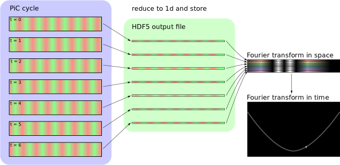
Figure 1: Sketch of the analysis pipeline.

After the numerical simulation has been performed, it is necessary to extract properties of the wave modes and compare with the expected behavior. To this end it is very useful to plot the energy density of a field component as a function of $k$ and $\omega$. The energy density is sharply localized along linear wave modes and characteristic frequencies (e.g. the low frequency cutoff of the electromagnetic mode) can easily and reliably be extracted.

Fig. 1 shows a sketch of the analysis that is performed. For the following explanation, we assume that we are interested in one component of the transverse electric field, other field components work analogously. Depending on the simulation code, $E_{\mathrm{x}}(z,t)$ or possibly $E_{\mathrm{x}}(x,y,z,t)$ is computed in every time step. This quantity is stored along with the necessary meta-data in a HDF5 file for later analysis.

As I/O can be a bottleneck for the simulation code, it is desirable to reduce overall output requirements. For the study of low frequency wave modes, it is usually sufficient to perform output every $N_{\mathrm{io}}$ time steps as long as

$$\frac{\pi}{N_{\mathrm{io}}\,\Delta t}=\frac{\pi}{\Delta t_{\mathrm{io}}}<\omega$$ (57)

holds for the highest frequency $\omega$ that is of interest. Similarly, it should be considered whether the code can average over the negligible directions before performing output.

In post-processing, $E_{\mathrm{x}}(z,t)$ is Fourier transformed in space and time to yield $\tilde{E}_{\mathrm{x}}(k_{z},\omega)$. To scale the axis correctly, it is useful to know that the frequency range one gets out of snapshots that are separated by $\Delta t_{\mathrm{io}}$ is $0\dots\pi/t_{\mathrm{io}}$ in steps of $\pi/T_{\mathrm{sim}}$. The range in $k$ is $-\pi/\Delta x\dots\pi\Delta x$. In most cases it is advisable to rescale from the units used in the code – CGS with values in in 1/s and 1/cm for the codes used here – to plasma scales such as $\omega_{\mathrm{p}}$, $\Omega_{\mathrm{c,e}}$ before plotting.

5.1 Test 1: Electromagnetic Mode

The cheapest test is designed to capture the electromagnetic mode. It does not use any background magnetic field and the size is given in Tab. 3.

simulation domain	$L_{z}$	$2048\,\Delta x$
simulation duration	$T_{\mathrm{sim}}$	$200\,\omega_{p,e}^{-1}$
		$10400\,\Delta t$

Table 3: Simulation size to study the electromagnetic mode.

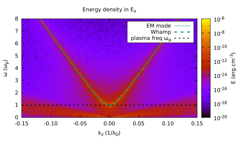
Figure 2: Energy density in one transverse component of the electric field as simulated by the electromagnetic plasma model. The electromagnetic mode is clearly visible, including the cutoff at the plasma frequency $\omega_{\mathrm{p}}$. The simulation parameters can be found in Tabs. 1 and 3, but the simulation is performed without a magnetic field.

Fig. 2 shows that the energy is mostly concentrated along the dispersion relation predicted by cold plasma theory (given by Eq. (31), shown as a dashed line) and has a cutoff at the plasma frequency $\omega_{\mathrm{p}}$, which is indicated by the horizontal dashed line. Predictions for the absolute magnitude and the low frequency noise are given in [30], but are not discussed here.

This mode is the cheapest way to determine the plasma frequency from the simulated data and compare it to the desired value from the simulation input. Many numerical problems (wrong normalization, errors in the charge or current deposition, problems in the particle pusher) can alter this mode, so it is ideally suited as a quick regression check after code modifications.

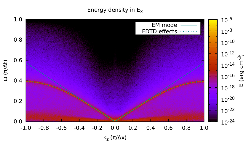
Figure 3: Spectral energy density up to the resolution limits permitted by the finite cell size and time step length. This plot uses data from the same simulation as Fig. 2. At high frequencies and large $k$ close to $\pm\pi/\Delta x$, significant numerical dispersion is visible.

At large $k$ – closer to the Nyquist limit imposed by the grid size $\Delta x$ – numerical dispersion effects occur that result from the discrete Maxwell solver in the simulation code. Fig. 3 shows this effect of the FDTD algorithm that is used to solve Maxwell’s equations in time. The modified dispersion relation is given by Eq. (54), in good agreement with our results.

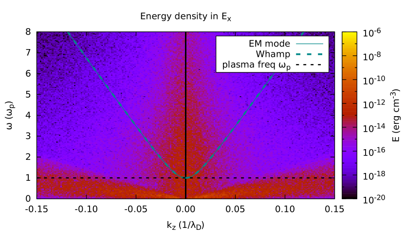
Figure 4: Energy density in one component of the radiation-free plasma model. For this plot the same parameters listed in Tabs. 1 and 3 were used, with the exception of the background magnetic field. Compared to Fig. 2, the electromagnetic mode is missing.

In the radiation free plasma model, the electromagnetic mode is explicitly removed. The remaining part of the transverse spectrum is shown in Fig. 4. No well defined mode is left in the unmagnetized case. At small $\omega$ and low phase velocities, a diffuse mode is visible that can be identified as ion acoustic waves. These, however, have a broadband spectrum without sharp features that would provide a good test problem.

The increase in noise at low $k$ can be attributed to a well known numerical instability at scales larger than the electron skin depth in the radiation-free plasma model. This instability can be removed through the introduction of a shift constant in the equation for the transverse electric field, but some noise remains (see [26] for details).

5.2 Test 2: High frequency L and R Modes

The addition of a background magnetic field (of 2.843 mT in this test problem) along the $z$ direction splits the electromagnetic mode into two modes with circular polarization.

To study polarization properties of the waves, one switches from a standard Cartesian basis (with transverse components $\hat{x},\hat{y}$) to a circular basis. In plasma physics phase convention, the new basis vectors are given by

$$\hat{l} =\frac{1}{\sqrt{2}}\left(\hat{x}-\imath\,\hat{y}\right)\quad,$$ (58)

$$\hat{r} =\frac{1}{\sqrt{2}}\left(\hat{x}+\imath\,\hat{y}\right)\quad.$$ (59)

Instead of performing the analysis that is sketched in Fig. 1 on a field component in the Cartesian basis (e.g. $E_{\mathrm{x}}(z,t)$), it is possible to combine $E_{\mathrm{x}}(z,t)$ and $E_{\mathrm{y}}(z,t)$ in the following way:

$$E_{\mathrm{l,r}}=\frac{1}{\sqrt{2}}\left(E_{\mathrm{x}}(z,t)\mp\imath\,E_{\mathrm{y}}(z,t)\right)\quad.$$ (60)

As usual, a Fourier transform in space and time is performed to yield $\tilde{E}_{\mathrm{l,r}}(k_{\mathrm{z}},\omega)$. Figs. 5 and 6 how the spectral energy density $|\tilde{E}_{\mathrm{l,r}}|^{2}$ respectively.

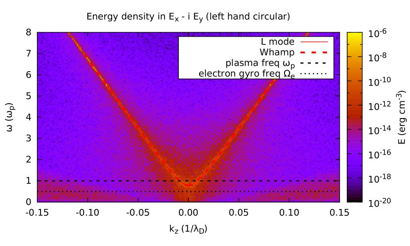
Figure 5: Energy density in the left handed circularly polarized component of the electric field produced by the electromagnetic plasma model. This plot is based on parameters given in Tabs. 1 and 3. The spectral energy density is concentrated along the high frequency branch of the L mode, propagating along the background magnetic field.

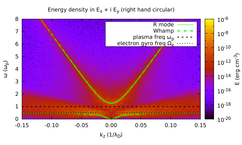
Figure 6: Energy density in the right handed circularly polarized component of the electric field produced by the electromagnetic plasma model. This plot uses the same parameters as Fig. 5, but the simulation results are combined differently to display the other circular polarization basis. Both high and low frequency branches of the R mode are visible.

In the circular basis only the wave modes with the matching circular polarization appear, thus confirming that the numerical implementation reproduces the expected polarization properties. Both modes follow the analytically predicted dispersion relation given in Eq. (34). The cutoff is shifted (away from the cutoff at $\omega_{\mathrm{p}}$ in the unmagnetized case) by about $\pm 1/2\,\Omega_{\mathrm{c,e}}$ as expected.

In the right hand polarization, shown in Fig. 6, two additional features are visible. One is a low frequency component with a resonance at $\Omega_{\mathrm{c,e}}$, which will be studied in more detail in a following test. The other feature is a triangular region of fluctuations that is caused by gyrating electrons. Within that region that is centered on $\Omega_{\mathrm{c,e}}$ and bounded by approximately $\pm 3v_{\mathrm{th,e}}\,k$, the dispersion relation of the R mode is modified. At larger $k$ the wave is absorbed. Both effects are captured by WHAMP and studied in more detail in Test 6.

5.3 Test 3: Extraordinary Mode

Keeping the background magnetic field along $z$ and rotating the simulation box to point along $x$, allows to study waves that propagate across the magnetic field. (Alternatively, one can change the direction of the magnetic field, in which case field components switch behavior.)

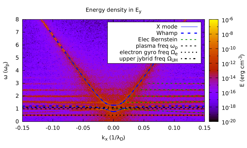
Figure 7: Energy density in the electric field component that is perpendicular to both the background magnetic field and the propagation direction. The plot shows simulation results from the electromagnetic plasma model with parameters given in Tabs. 1 and 3. Both branches of the X mode are clearly visible. Due to the finite temperature, harmonics of the electron gyro frequency and the first few electron Bernstein modes are also visible.

As expected, the field component perpendicular to $k$ and $B_{0}$ shows the extraordinary mode. Both the high frequency branch above the upper hybrid frequency and the branch close to the plasma frequency show the expected dispersion relation given in Eq. 39. Thermal effects are not important for this mode, as can be seen by the excellent agreement between the predictions of cold plasma theory and the numerical solution by WHAMP that includes finite temperature effects.

Fig. 7 also shows approximately horizontal features at harmonics of the electron gyro frequency. These are due to electron Bernstein waves which can only be explained by the thermal effects and are studied in more detail in Test 7.

5.4 Test 4: Langmuir Mode

This test problem focuses on longitudinal waves which, in the unmagnetized case, are represented by the Langmuir mode. As mentioned previously, this mode is a result of plasma oscillations in a plasma of finite temperature. Consequently, it can be used to determine the thermal speed of the electrons $v_{\mathrm{th,e}}$ and thereby the temperature $T_{\mathrm{e}}$. This is of interest in codes that start with all particles at rest and rely on the initial fluctuations in the charge density to generate a thermal velocity distribution.

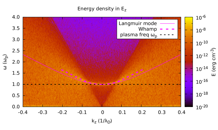
Figure 8: Energy density in the longitudinal component of the electric field. The simulation was performed with using the electromagnetic plasma model and the parameters given in Tabs. 1 and 3, but without background magnetic field. At not too large $k$, the Langmuir mode is clearly visible.

Fig. 8 compares the energy distribution in the longitudinal electric field with the expected dispersion relation of a Langmuir mode in a plasma of the same temperature that was used to generate the initial velocity distribution. For small $k$, the agreement with the analytic prediction is very good. At intermediate $k$, there are deviations from the analytic prediction due to the rather large electron temperature. WHAMP, however, is able to accurately predict the behavior of the plasma. At large $k$, the wave is strongly damped and not visible in the spectral energy distribution. This effect is also predicted by WHAMP, but missing from the analytical dispersion relation given in Eq. (47).

Figure 9: Energy density in the longitudinal component of the electric field. The setup and parameters are identical to Fig. 8 but the electric field is computed by the spectral solver that is used in both the radiation-free and the electrostatic plasma model.

Fig. 9 shows the longitudinal electric field, as determined by the spectral solver that is used in the radiation-free plasma model as well as the electrostatic plasma model in ACRONYM. The gap at $k=0$ is an artifact of the spectral solver that was mentioned before. At all other $k$ the match to the electromagnetic plasma model and the prediction from theory is very good.

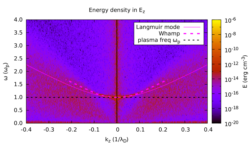
Figure 10: Plot of longitudinal perturbations in the electric field for the alternative implementation of the electrostatic plasma model using the VHS technique. See page 4.4 for a description and Tabs. 1 and 3 for parameters.

Fig. 10 shows the longitudinal electric field for the alternative implementation of the electrostatic plasma model using the VHS technique. This method has a very low level of intrinsic noise. To make the Langmuir mode visible, the initial density of each species was randomly perturbed on every point of the phase space grid by plus or minus five percent. This reproduces the Langmuir mode at about the same strength as it appears in the PiC simulations.

Very visible at least in Fig. 8 and 9 and still recognizable in Fig. 10 is the change in the broadband noise floor that is caused by thermal electrons and reaches up to

$$\omega=3\sqrt{2}\,v_{\mathrm{th,e}}\,k\quad.$$ (61)

The reduction of this noise floor by at least four orders of magnitude is the main reason to consider implementing the electrostatic plasma model using the VHS method.

The hybrid plasma models do not include kinetic effects of the electrons and assume instantaneous neutrality which, therefore, removes the Langmuir mode as well as the thermal broadband noise.

5.5 Test 5: Bernstein Modes

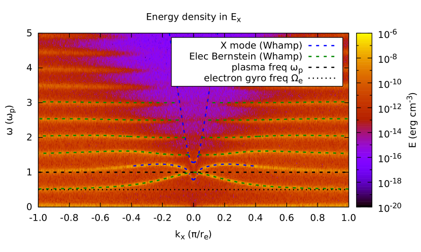
Figure 11: Energy density in the longitudinal component of the electric field. The simulation was performed using the electromagnetic plasma model, using parameters from Tabs. 1 and 3. The first few electron Bernstein modes are clearly visible.

Fig. 11 shows the electron Bernstein modes described in Sec. 3.5. A comparison with theoretical predictions is hampered by the complicated dispersion relations of these modes. Using the leading terms of the infinite sums, it is possible to plot the first few modes. The figure also contains some influence from the X mode that has a longitudinal components at low $k$.

Figure 12: Energy density in the longitudinal component of the electric field. Unlike Fig. 11, the field is computed using the spectral solver used by the radiation-free and the electrostatic plasma models.

Fig. 12 shows the behavior in the electrostatic model with a static background magnetic field. Again we see a spectral hole at $k=0$. Compared to Fig. 11, no remnants of the X mode are visible here.

The absence of kinetic electrons in the hybrid models, carrying individual gyro phases, removes electron Bernstein modes.

5.6 Test 6: Low Frequency R Mode

So far all simulations were as cheap as Test 1. To analyze the low frequency regime, some more effort is required. Tab. 4 lists the changes to the simulation parameters.

simulation domain	$L_{\mathrm{z}}$	$8192\,\Delta x$
simulation duration	$T_{\mathrm{sim}}$	$1000\,\omega_{\mathrm{p,e}}^{-1}$
		$52000\,\Delta t$

Table 4: Simulation size to study the low frequency R mode.

When we run the simulation using those parameters and plot the result, we again find the L and R mode. Limiting ourselves to frequencies up to the electron gyro frequency and filtering for right hand circular polarization, we get Fig. 13.

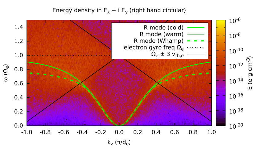
Figure 13: Energy density in the right handed circularly polarized part of the electric field. Similar to Fig. 6, the electric field is computed from the electromagnetic plasma model, but this time with the parameters given in Tabs. 1 and 4 to reach the low frequency regime. As expected, the low frequency branch of the R mode is visible, including the frequency range of whistler waves.

Fig. 13 is dominated by the low frequency branch of the R mode which contains a region where $\omega$ depends quadratically on $k$. These waves would usually be classified as whistler waves.

For larger $k$, the group velocity drops again as the wave comes closer to the resonance at $\Omega_{\mathrm{c,e}}$. In this region, a deviation can be seen between the prediction for a cold plasma and the mode in the simulated plasma of finite temperature. Using either the prediction of [31] for a warm plasma or the linearized equations of WHAMP, this effect can be predicted correctly. Both approaches, however, require to numerically solve for the dispersion relation.

For even larger $k$, the mode is damped away by gyrating particles, which is also predicted for warm plasmas. The gyrating electrons generate noise cones around the electron gyro frequency that are clearly visible. The opening angle of the cones corresponds to roughly $3\sqrt{2}~{}v_{\mathrm{th,e}}~{}k$.

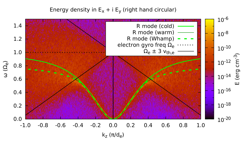
Figure 14: Energy density in the right handed circularly polarized part of the electric field. Unlike Fig. 13 the field is computed using the radiation-free plasma model, but otherwise using the same parameters.

Fig. 14 shows the low frequency modes that are right handed circularly polarized from a radiation free plasma model. Unlike the high frequency branches of L and R mode that are removed when the electromagnetic radiation is removed, the low frequency branches still exist and show the same features as in an full electromagnetic plasma model.

In an electrostatic plasma model, these waves are missing because no transverse fields exist.

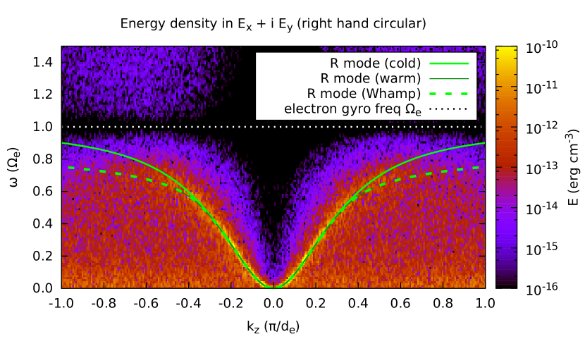
Figure 15: Energy density in the right handed circularly polarized part of the electric field. In this figure the field is computed from the hybrid model with electron inertia. Compared to Fig. 13, the noise cones around the gyro frequency of electrons are missing.

As Fig. 15 shows, the noise cones of gyrating electrons – a purely kinetic effect – are missing in a model that uses an electron fluid. The low frequency branch of the R mode, however, still exists and shows the correct dispersion relation. This is not surprising as the wave is carried by electrons but can be derived in the (fluid-like) plasma theory. The gyro frequency of electrons can be estimated from the spectral gap in the noise.

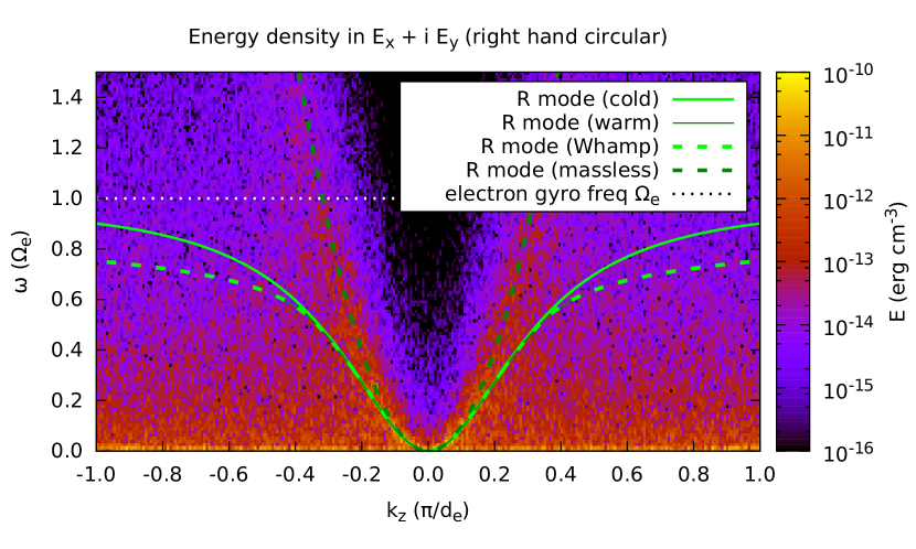
Figure 16: Energy density in the right handed circularly polarized part of the electric field. This time a hybrid model with massless electrons is used to compute the electric field. The dispersion relation of the low frequency R mode is significantly modified by this model as a comparison with Figs. 13 to 15 shows.

Fig. 16 shows the right hand circular mode in the limit $m_{\mathrm{e}}\rightarrow 0$. For small $k$, the mode is unchanged by the lack of electron inertia, but at larger $k$ it lacks the resonance at the electron gyro frequency, which is not well defined without electron mass.

Normalizing in the same way as used for the plot ${\omega=\tilde{\omega}\,\Omega_{\mathrm{c,e}}}$ and ${k=\tilde{k}\,\pi/d_{\mathrm{e}}}$ simplifies the dispersion relation given in Eq. 38 significantly:

$$\tilde{\omega}=\pi^{2}\,\tilde{k}^{2}\quad,$$ (62)

The plot of the spectral energy density indeed shows that the wave mode follows this dispersion relation even for frequencies $\omega$ larger than the electron gyro frequency.

5.7 Test 7: Ion Bernstein Modes

electron plasma frequency	$\omega_{\mathrm{p,e}}$	$1.000\cdot 10^{9}\,\mathrm{rad}/\mathrm{s}$
electron gyro frequency	$\Omega_{\mathrm{c,e}}$	$2.144\cdot 10^{8}\,\mathrm{rad}/\mathrm{s}$
electron thermal speed	$v_{\mathrm{th,e}}$	0.021 c
mass ratio	$m_{\mathrm{i}}/m_{\mathrm{e}}$	1836
temperature	$T$	2.71 MK
Debye length	$\lambda_{\mathrm{D}}$	0.641 cm
grid size	$\Delta x$	0.454 cm
electron gyro radius	$r_{\mathrm{e}}$	2.993 cm
magnetic field	$B_{0}$	1.219 mT
		12.19 G
Alfvén speed	$v_{\mathrm{A}}$	0.005 c
simulation domain	$L_{x}$	$16384\,\Delta x$
simulation duration	$T_{\mathrm{sim}}$	$150\,\Omega_{c,i}^{-1}$

Table 5: Simulation parameters used for the ion Bernstein modes.

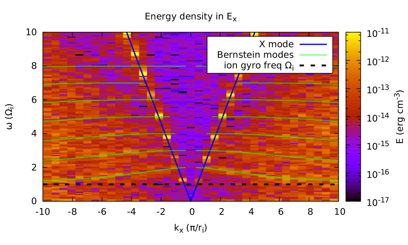
Figure 17: Energy density in the longitudinal component of the electric field. The field has been obtained from the electromagnetic plasma model using the parameter set given in Tab. 5.

Fig. 17 shows the result of test 7 using the electromagnetic plasma model. The simulation is computationally expensive and quite noisy. The X mode is clearly visible. At smaller phase speeds, ion Bernstein modes are visible. Better resolution and lower noise levels (e.g. through a larger number of particles per cell) would be required to make this an efficient test, but would increase the computational cost even further.

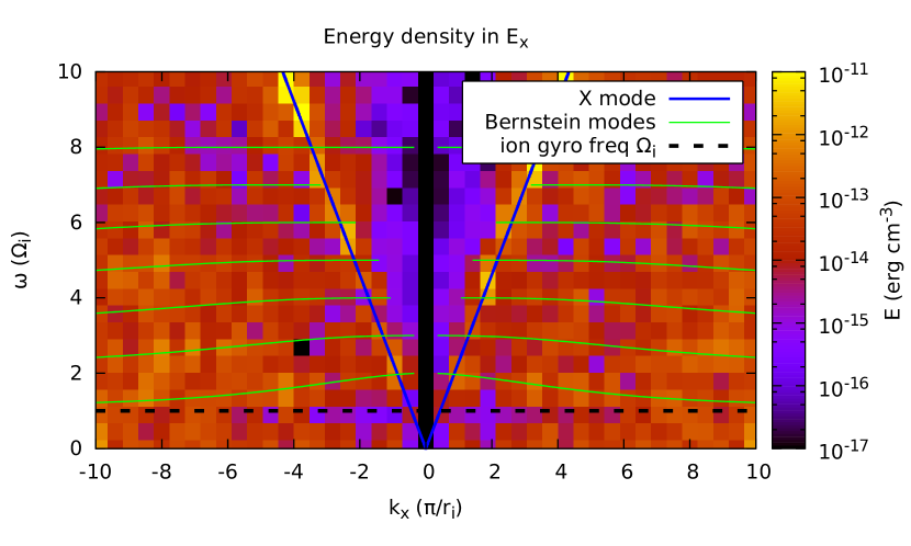
Figure 18: Energy density in the longitudinal component of the electric field. The field has been obtained from the spectral solver used for the radiation-free plasma model.

Fig. 18 shows the result of the spectral solver as used in the radiation-free plasma model. As usual with this solver, a hole in the spectral energy density appears at $k=0$. This plasma model allows larger time steps than the electromagnetic model, but the simulation is still too expensive to make an efficient test problem.

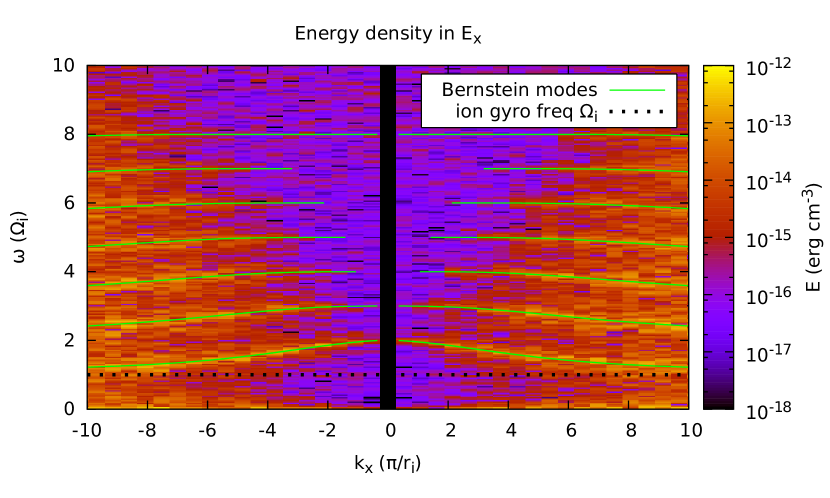
Figure 19: Energy density in the longitudinal component of the electric field. The field has been obtained from the spectral solver used for the electrostatic plasma model using the parameter set given in Tab. 5. The only visible wave modes are ion Bernstein waves.

Fig. 19 shows the result of the spectral solver as used in the electrostatic plasma model. This model does not include the X mode and allows much larger time steps, which reduces computational expense. Additionally, a single time is cheaper than in the radiation-free model and the test does not rely on the transverse field components that are missing in the electrostatic model.

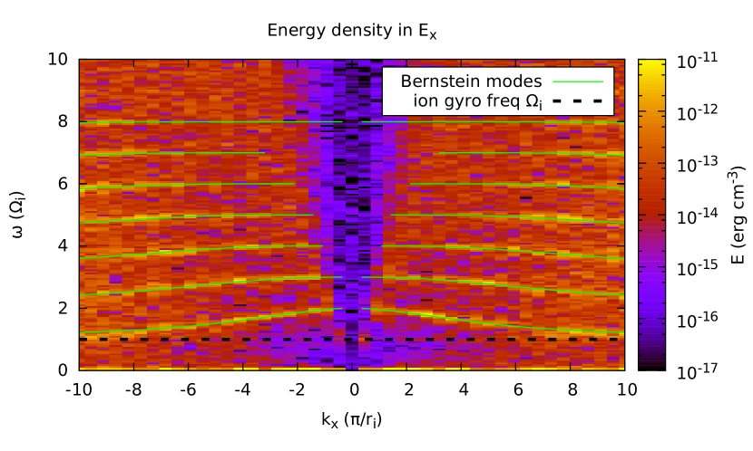
Figure 20: Energy density in the longitudinal component of the electric field. The plot is based on the hybrid model with electron inertia and the parameter set given in Tab. 5.

Fig. 20 shows the output of the hybrid plasma model including effects of electron inertia. In this model, ions are treated as kinetic particles and, as expected, ion Bernstein modes are visible. Note the reappearance of the X mode as an enhanced band of noise at relatively large phase velocities.

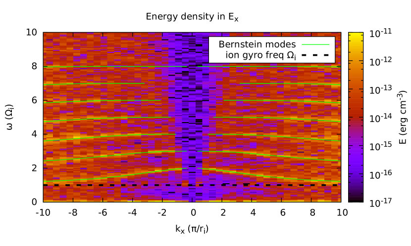
Figure 21: Energy density in the longitudinal component of the electric field. The hybrid model used the parameter set given in Tab. 5 and massless electrons. The case including electron inertia can be found in Fig. 20.

Fig. 21 shows the hybrid plasma models without electron inertia. The ion Bernstein modes are dominated by ion kinetic effects and remain unchanged. Given that this plasma model admits a only limited number of modes, this is probably the most relevant test problem for it.

5.8 Test 8: Low Frequency L Mode

Resolving low frequency L modes, as done in Sec. 5.6 for their right handed counterparts, would require another large increase in effort. (One needs 1836 times as many time steps to resolve the lower gyro frequency and $\sqrt{1836}$ more cells to capture the larger gyro radius.) The only feasible way is to reduce the mass ratio between protons and electrons. Low mass ratios result in possibly unrealistic high Alfvén speeds if the magnetic field is not adjusted. Tab. 6 shows parameters that are a reasonable tradeoff and allow a glimpse at this wave mode.

mass ratio	$m_{\mathrm{i}}/m_{\mathrm{e}}$	18.36
Alfvén speed	$v_{\mathrm{A}}$	0.117 c
simulation domain	$L_{\mathrm{z}}$	$16384\,\Delta x$
simulation duration	$T_{\mathrm{sim}}$	$4000\,\omega_{\mathrm{p,e}}^{-1}$
		$208000\,\Delta t$
particle updates		$3.5\cdot 10^{12}$

Table 6: Simulation size to study the low frequency L mode.

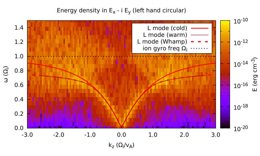
Figure 22: Energy density in the left handed circularly polarized part of the electric field. The plot is based on a simulation using the electromagnetic plasma model and parameters given in Tab. 6. As expected, the low frequency L mode is visible as well as noise cones produced by gyrating ions.

Running the simulation with those parameters and plotting the spectral energy density of left handed modes results in Fig. 22. The low frequency branch of the L mode is clearly visible. For small $k$, it matches well the prediction for a cold plasma. For intermediate $k$, effects of the finite temperature have to be included to explain the simulation results. At higher $k$, the mode is damped away by gyrating protons that are visible as noise cones. These cones are analogous to the cones generated by gyrating electrons, but occur on ion scales, i.e. they are centered on the gyro frequency of the ions and the opening is determined by the thermal speed of ions.

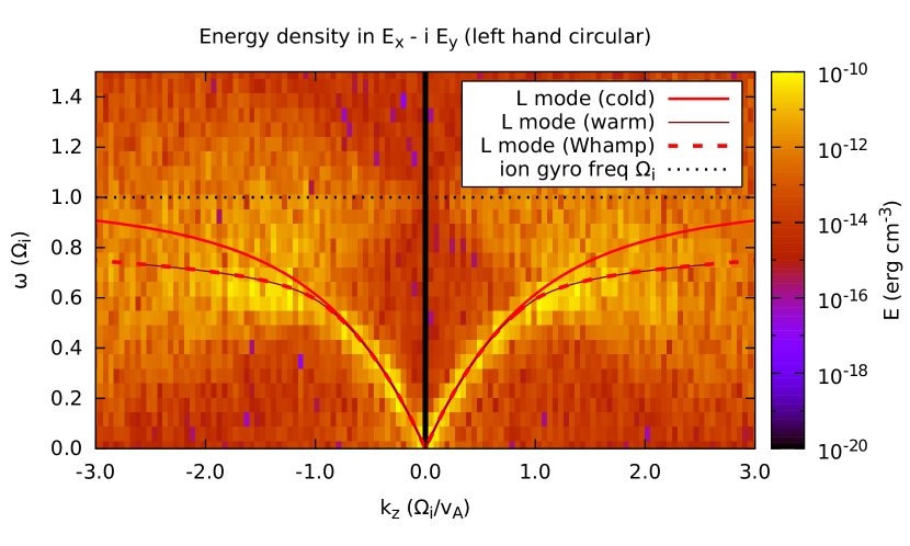
Figure 23: Energy density in the left handed circularly polarized part of the electric field obtained from the radiation-free plasma model. The simulation parameters can be found in Tab. 6.

In Fig. 23 it can be seen that the left handed low frequency waves survive in the radiation-free plasma, the same as the right handed counterparts.

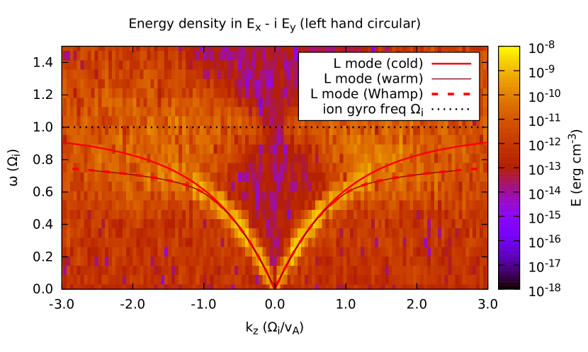
Figure 24: Energy density in the left handed circularly polarized part of the electric field. Again parameters from Tab. 6, but this time for a hybrid model with electron inertia. The ions are still treated kinetically and consequently the low frequency L mode and the noise cones are retained.

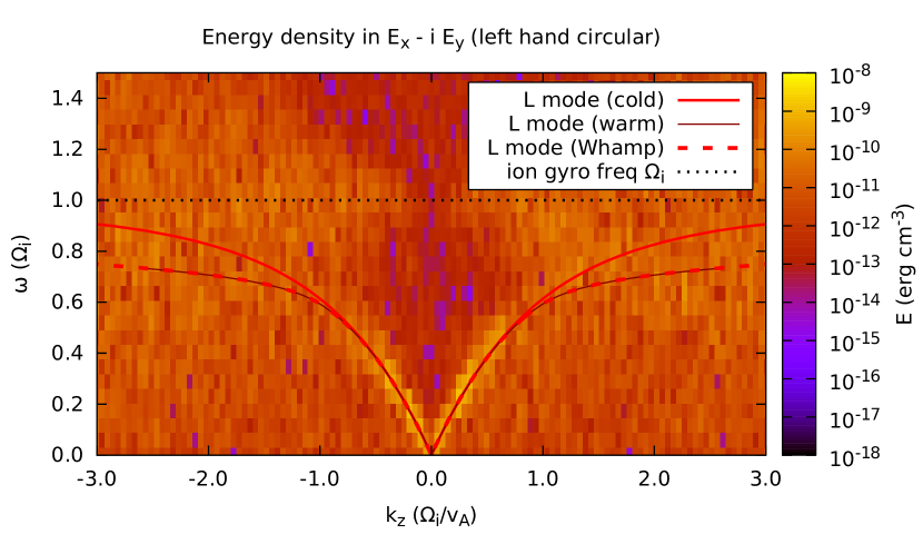
Figure 25: Energy density in the left handed circularly polarized part of the electric field. Compared to Fig. 24 electron inertia has been removed.

Figs. 24 and 25 show that the low frequency L mode branches exist basically unaltered without kinetic electrons. The noise cones of gyrating ions are unaffected unlike Fig. 15.

6 Conclusions

In this work we proposed a set of test problems suitable for a wide range of kinetic plasma models and provided reference results based on our numerical codes. Those tests are based on a set of different plasma wave modes and are useful to check quickly and conveniently the correct implementation of different plasma models, including the correct interaction of the different parts of the simulation program handling particles and electromagnetic fields.

Plasma Model	Wave Mode
	EM	HF L/R	X	Langmuir	EB	LF R	IB	LF L
Electromagnetic	X	X	X	X	X	X	$	$
Radiation-free	-	-	-	X	X	X	$	$
Electrostatic	-	-	-	X	X	-	X	-
Hybrid w/ inertia	-	-	-	-	-	X	X	X
Hybrid w/o inertia	-	-	-	-	-	$\scriptstyle\sim$	X	X

Table 7: Suitability of modes for different plasma models. EB and IB stand for Bernstein modes of electrons and ions, respectively. Cases indicated by ’X’ allow for an effective test. An entry of ’-’ indicates that the wave mode is not suitable for testing implementations of this plasma model. The four cases that are marked $ are in principle suitable, but computationally expensive. The one special case indicated with $\scriptstyle\sim$ is explained in the text.

Tab. 7 shows which wave modes are suitable to test codes implementing different plasma models. Listed from left to right are the electromagnetic mode from Sec. 5.1, left and right hand circular wave modes at or above the plasma frequency (Sec. 5.2), the extraordinary mode (Sec. 5.3), the Langmuir mode (Sec. 5.4), electron Bernstein modes (Sec. 5.5), low frequency waves with right hand circular polarization (Sec. 5.6), ion Bernstein modes (Sec. 5.7) and low frequency left hand circular polarization (Sec. 5.8). Listed on the left hand side are the different plasma models – from top to bottom –, the electromagnetic model (Sec. 2.1), the radiation-free model (Sec. 2.2), the electrostatic model (Sec. 2.3) and the model using an implicit electron fluid – either with or without electron inertia – described in Sec. 2.4.

Wave modes that provide suitable test problems for the chosen plasma model are indicated with ’X’. If a ’-’ is listed, the wave mode is not present or usable in the plasma model. For two plasma models, the low frequency left hand circularly polarized waves and the ion Bernstein modes are marked with $. These waves do exist in the electromagnetic and radiation-free plasma model and show the properties expected from cold plasma theory. In principle, these waves could be used to test the simulation code, e.g. by extracting the gyro frequency of ions or the Alfvén velocity. Simulations with sufficient resolution are, however, computationally very expensive. Given that these plasma models admit a large number of alternative wave modes, it is better to choose an alternative test problem unless low frequency properties of the ions are explicitly needed. A special case (indicated by ’$\scriptstyle\sim$’), occurs for low frequency right hand circularly polarized waves in the hybrid model without electron inertia. As shown in Fig. 16, such a wave mode does exist, however, the dispersion relation is modified compared to all other plasma models used here. In particular the resonance at the electron gyro frequency is missing, as it has been ordered out of the model and cannot be used for comparison purposes. Using the modified dispersion relation in Eq. 38, it is possible to recover the combination of magnetic field and electron density. Given the limited number of suitable wave modes in this hybrid plasma model, right hand circularly polarized waves are still an important test problem, but analysis requires extra attention, and direct comparison with other plasma models is difficult.

References

- [1] J. Birn, J. F. Drake, M. A. Shay, B. N. Rogers, R. E. Denton, M. Hesse, M. Kuznetsova, Z. W. Ma, A. Bhattacharjee, A. Otto, P. L. Pritchett, Geospace environmental modeling (GEM) magnetic reconnection challenge, Journal of Geophysical Research: Space Physics 106 (A3) (2001) 3715–3719. doi:10.1029/1999JA900449.
- [2] A. M. Dimits, G. Bateman, M. A. Beer, B. I. Cohen, W. Dorland, G. W. Hammett, C. Kim, J. E. Kinsey, M. Kotschenreuther, A. H. Kritz, L. L. Lao, J. Mandrekas, W. M. Nevins, S. E. Parker, A. J. Redd, D. E. Shumaker, R. Sydora, J. Weiland, Comparisons and physics basis of tokamak transport models and turbulence simulations, Physics of Plasmas 7 (3) (2000) 969–983. doi:10.1063/1.873896.
- [3] G. L. Falchetto, B. D. Scott, P. Angelino, A. Bottino, T. Dannert, V. Grandgirard, S. Janhunen, F. Jenko, S. Jolliet, A. Kndl, B. F. McMillan, V. Naulin, A. H. Nielsen, M. Ottaviani, A. G. Peeters, M. J. Pueschel, D. Reiser, T. T. Ribeiro, M. Rmanelli, The European turbulence code benchmarking effort: turbulence driven by thermal gradients in magnetically confined plasmas, Plasma Physics and Controlled Fusion 50 (12) (2008) 124015.
- [4] T. Görler, N. Tronko, W. A. Hornsby, A. Bottino, R. Kleiber, C. Norscini, V. Grandgirard, F. Jenko, E. Sonnendrücker, Intercode comparison of gyrokinetic global electromagnetic modes, Physics of Plasmas 23 (7). doi:10.1063/1.4954915.
- [5] J. D. Jackson, Classical Electrodynamics, 3rd Edition, Wiley, New York, 1999.
- [6] J. A. Bittencourt, Fundamentals of Plasma Physics, 3rd Edition, Springer, 2004.
- [7] A. A. Vlasov, On high-frequency properties of electron gas, Journal of Experimental and Theoretical Physics 8 (3) (1938) 291–318.
- [8] H. A. Lorentz, La théorie électromagnétique de Maxwell et son application aux corps mouvants, Landmarks of science, E.J. Brill, 1892.
- [9] J. Maxwell, A dynamical theory of the electromagnetic field, Philosophical Transactions of the Royal Society of London 155 (1) (1865) 459–513.
- [10] C. K. Birdsall, A. B. Langdon, Plasma physics via computer simulation, 1st Edition, New York: Taylor and Francis, 2005.
- [11] T. B. Krause, A. Apte, P. J. Morrison, A unified approach to the Darwin approximation, Physics of Plasmas 14 (10) (2007) 102112. doi:10.1063/1.2799346.
- [12] C. G. Darwin, The dynamical motions of charged particles, Philosophical Magazine Series 5 39. doi:10.1080/14786440508636066.
- [13] L. Landau, On the vibrations of the electronic plasma, Journal of Experimental and Theoretical Physics 16 (7) (1946) 574–586.
- [14] H. E. J. Koskinen, Physics of space storms from the solar surface the Earth, Springer-Verlag, Berlin; heidelberg; London; Chichester, 2011. doi:10.1007/978-3-642-00319-6.
- [15] T. H. Stix, The Theory of Plasma Waves, McGawn-Hill, Inc., 1962.
- [16] S. V. Bulanov, F. Pegoraro, A. S. Sakharov, Magnetic reconnection in electron magnetohydrodynamics, Physics of Fluids B 4 (8) (1992) 2499–2508. doi:10.1063/1.860467.
- [17] D. Shaikh, Theory and simulations of whistler wave propagation, Journal of Plasma Physics 75 (2009) 117–132. doi:10.1017/S0022377808007198.
- [18] B. D. Fried, S. D. Conte (Eds.), The Plasma Dispersion Function, Academic Press, 1961. doi:10.1016/B978-1-4832-2929-4.50001-0.
- [19] J. M. Dawson, On landau damping, Physics of Fluids 4 (7) (1961) 869–874. doi:10.1063/1.1706419.
- [20] I. B. Bernstein, Waves in a plasma in a magnetic field, Phys. Rev. 109 (1958) 10–21. doi:10.1103/PhysRev.109.10.
- [21] D. Swanson, Plasma Waves, 2nd Edition, Series in Plasma Physics, Taylor & Francis, 2003.
- [22] P. Kilian, T. Burkart, F. Spanier, The influence of the mass ratio on particle acceleration by the filamentation instability, in: W. E. Nagel, D. B. Kröner, M. M. Resch (Eds.), High Performance Computing in Science and Engineering ’11, Springer, Berlin Heidelberg, 2012, pp. 5–13. doi:10.1007/978-3-642-23869-7.
- [23] T. Z. Esirkepov, Exact charge conservation scheme for particle-in-cell simulation with an arbitrary form-factor, Computer Physics Communications 135 (2) (2001) 144 – 153. doi:10.1016/S0010-4655(00)00228-9.
- [24] N. Jain, A. Das, P. Kaw, S. Sengupta, Nonlinear electron magnetohydrodynamic simulations of sausage-like instability of current channels, Physics of Plasmas 10 (1) (2003) 29–36. doi:10.1063/1.1523011.
- [25] K. Yee, Numerical solution of inital boundary value problems involving maxwell’s equations in isotropic media, Antennas and Propagation, IEEE Transactions on 14 (3) (1966) 302–307.
- [26] V. K. Decyk, Description of spectral particle-in-cell. codes in the upic framework, Presentation at ISSS-10 (2011).
- [27] D. Nunn, A novel technique for the numerical simulation of hot collision-free plasma; vlasov hybrid simulation, Journal of Computational Physics 108 (1) (1993) 180 – 196. doi:10.1006/jcph.1993.1173.
- [28] P. Muñoz, N. Jain, P. Kilian, J. Büchner, A new hybrid code (chief) implementing the inertial elecron fluid equation without approximation, In preparation.
- [29] K. Roennmark, Waves in homogeneous, anisotropic multicomponent plasmas (WHAMP), Tech. rep., Kiruna Geophysical Insitute (Jun. 1982).
- [30] A. G. Sitenko, Electromagnetic Fluctuations in Plasma, Academic Press, New York, 1967.
- [31] L. Chen, R. M. Thorne, Y. Shprits, B. Ni, An improved dispersion relation for parallel propagating electromagnetic waves in warm plasmas: Application to electron scattering, Journal of Geophysical Research: Space Physics 118 (5) (2013) 2185–2195. doi:10.1002/jgra.50260.