Infinite-sample consistent estimations of parameters of the Wiener process with drift

Abstract.

We consider the Wiener process with drift

$$dX_{t}=\mu dt+\sigma dW_{t}$$

with initial value problem $X_{0}=x_{0}$, where $x_{0}\in R$, $\mu\in R$ and $\sigma>0$ are parameters. By use values $(z_{k})_{k\in N}$ of corresponding trajectories at a fixed positive moment $t$, the infinite-sample consistent estimates of each unknown parameter of the Wiener process with drift are constructed under an assumption that all another parameters are known. Further, we propose a certain approach for estimation of unknown parameters $x_{0},\mu,\sigma$ of the Wiener process with drift by use the values $(z^{(1)}_{k})_{k\in N}$ and $(z^{(2)}_{k})_{k\in N}$ being the results of observations on the $2k$-th and $2k+1$-th trajectories of the Wiener process with drift at moments $t_{1}$ and $t_{2}$ , respectively.

1. Introduction

Following [1], the Wiener process with drift is used as a mathematical model described a random motion of a particle suspended in water which is being bombarded by water molecules. The temperature of the water will influence the force of the bombardment, and thus we need a parameter $\sigma$ to characterize this. Moreover, there is a water current which drives the particle in a certain direction, and we will assume a parameter $\mu$ to characterize the drift. To describe the displacements of the particle, the Wiener process can be generalized to the process

$(1.1)$ $$dX_{t}=\mu dt+\sigma dW_{t}$$

which has solution

$(1.2)$ $$X_{t}=x_{0}+\mu t+\sigma W_{t}$$

for $X_{0}=x_{0}$(see [1], p.11) . It is thus normally distributed with mean $x_{0}+\mu t$ and variance $\sigma^{2}t$, as follows from the properties of the standard Wiener process. This process has been proposed as a simplified model for the membrane potential evolution in a neuron.

The parameters in (1.1)-(1.2) have the following sense:

(i) $\mu$ represents the equilibrium or mean value supported by fundamentals (in other words, the central location) and called a parameter of the drift in Wiener model with drift ;

(ii) $\sigma$ is a parameter of the bombardment force in Wiener model with drift ;

(iii) $x_{0}$ is an initioal position of the particle suspended in water in Wiener model with drift ;

(iv) $x_{t}$ is a position of the particle suspended in water in Wiener model with drift at moment $t>0$;

The purpose of the present paper is to introduce a new approach which by use values $(z_{k})_{k\in N}$ of corresponding trajectories at a fixed positive moment $t$, will allows us to construct a consistent estimate for each unknown parameter of theWiener model with drift under an assumption that all another parameters are known. Note that analogous problem has been considered by L.Labadze and G. Pantsulaia for Ornstein-Uhlenbeck’s stochastic process ( cf. [2]).

The rest of the present paper is the following:

In Section 2 we consider some auxiliary notions and facts from the theory of mathematical statistics and probability.

In Section 3 we present the constructions of consistent and infinite-sample consistent estimates for unknown parameters of the Wiener model with drift.

In Section 4 we present simulations and animations of the Wiener model with drift.

In Section 5 we propose a certain approach for estimation of unknown parameters $x_{0},\mu,\sigma$ of the Wiener process with drift by use the values $(z^{(1)}_{k})_{k\in N}$ and $(z^{(2)}_{k})_{k\in N}$ being the results of observations on the $2k$-th and $2k+1$-th trajectories of the Wiener process with drift at moments $t_{1}$ and $t_{2}$ , respectively.

2. Some auxiliary notions and facts

We begin this subsection by the following definition.

Let $\{\mu_{\theta}:\theta\in R\}$ be a family Borel probability measures in $R$. By $\mu_{{\theta}}^{N}$ we denote the $N$-power of the measure $\mu_{\theta}$ for $\theta\in R$.

Definition 2.1. A Borel measurable function $T_{n}:R^{n}\to R~{}(n\in N)$ is called a consistent estimator of a parameter $\theta$ (in the sense of everywhere convergence) for the family $(\mu_{\theta}^{N})_{\theta\in R}$ if the following condition

$$\mu_{\theta}^{N}(\{(x_{k})_{k\in N}:~{}(x_{k})_{k\in N}\in R^{N}~{}\&~{}\lim_{n\to\infty}T_{n}(x_{1},\cdots,x_{n})=\theta\})=1$$

holds true for each $\theta\in R$.

Definition 2.2. A Borel measurable function $T_{n}:R^{n}\to R~{}(n\in N)$ is called a consistent estimator of a parameter $\theta$ (in the sense of convergence in probability) for the family $(\mu_{\theta}^{N})_{\theta\in R}$ if for every $\epsilon>0$ and $\theta\in R$ the following condition

$$\lim_{n\to\infty}\mu_{\theta}^{N}(\{(x_{k})_{k\in N}:~{}(x_{k})_{k\in N}\in R^{N}~{}\&~{}|T_{n}(x_{1},\cdots,x_{n})-\theta|>\epsilon\})=0$$

holds.

Definition 2.3. A Borel measurable function $T_{n}:R^{n}\to R~{}(n\in N)$ is called a consistent estimator of a parameter $\theta$ (in the sense of convergence in distribution ) for the family $(\mu_{\theta}^{N})_{\theta\in R}$ if for every continuous bounded real valued function $f$ on $R$ the following condition

$$\lim_{n\to\infty}\int_{R^{N}}f(T_{n}(x_{1},\cdots,x_{n}))d\mu_{\theta}^{N}((x_{k})_{k\in N})=f(\theta)$$

holds.

Remark 2.1 Following [3] (see, Theorem 2, p. 272), for the family $(\mu_{\theta}^{N})_{\theta\in R}$ we have:

(a) an existence of a consistent estimator of a parameter $\theta$ in the sense of everywhere convergence implies an existence of a consistent estimator of a parameter $\theta$ in the sense of convergence in probability;

(b) an existence of a consistent estimator of a parameter $\theta$ in the sense of convergence in probability implies an existence of a consistent estimator of a parameter $\theta$ in the sense of convergence in distribution.

Definition 2.4 Following [4], the family $(\mu_{\theta}^{N})_{\theta\in R}$ is called strictly separated if there exists a family $(Z_{\theta})_{\theta\in R}$ of Borel subsets of $R^{N}$ such that

(i) $\mu_{\theta}^{N}(Z_{\theta})=1$ for $\theta\in R$;

(ii) $Z_{\theta_{1}}\cap Z_{\theta_{2}}=\emptyset$ for all different parameters $\theta_{1}$ and $\theta_{2}$ from $R$.

(iii) $\cup_{\theta\in R}Z_{\theta}=R^{N}.$

Definition 2.5. Following [4], a Borel measurable function $T:R^{N}\to R$ is called an infinite sample consistent estimator of a parameter $\theta$ for the family $(\mu_{\theta}^{N})_{\theta\in R}$ if the following condition

$$(\forall\theta)(\theta\in R\rightarrow\mu_{\theta}^{N}(\{(x_{k})_{k\in N}~{}:~{}(x_{k})_{k\in N}\in R^{N}~{}\&~{}T((x_{k})_{k\in N})=\theta\})=1)$$

holds.

Remark 2.2. Note that an existence of an infinite sample consistent estimator of a parameter $\theta$ for the family $(\mu_{\theta}^{N})_{\theta\in R}$ implies that the family $(\mu_{\theta}^{N})_{\theta\in R}$ is strictly separated. Indeed, if we set $Z_{\theta}=\{(x_{k})_{k\in N}:(x_{k})_{k\in N}\in R^{N}~{}\&~{}T((x_{k})_{k\in N})=\theta\}$ for $\theta\in R$, then all conditions in Definition 2.4 will be satisfied.

In the sequel we will need the well known fact from the probability theory (see, for example, [3], p. 390).

Lemma 2.1. (Kolmogorov’s strong law of large numbers) Let $X_{1},X_{2},...$ be a sequence of independent identically distributed random variables defined on the probability space $(\Omega,\mathcal{F},P)$. If these random variables have a finite expectation $m$ (i.e., $E(X_{1})=E(X_{2})=...=m<\infty$), then the following condition

$$P(\{\omega:\lim_{n\to\infty}n^{-1}\sum_{k=1}^{n}X_{k}(\omega)=m\})=1$$

holds true.

3. Estimation of parameters of Wiener process with drift

3.1. Estimation of a parameter of the bombardment force $\sigma$ in Wiener model with drift

The purpose of the present subsection is to estimate a parameter of the bombardment force $\sigma$ by water molecules acting on a particle suspended in water under assumption that we know results of observations on placements of the particle at moment $t_{0}$, a parameter of the drift $\mu$ and an initial position $x_{0}$.

Theorem 3.1.1  For $t>0$, $x_{0}\in R$, $\mu\in R$ and $\sigma>0$, let’s $\gamma_{(t,x_{0},\mu,\sigma)}$ be a Gaussian probability measure in $R$ with the mean $m_{t}=x_{0}+\mu t$ and the variance $\sigma_{t}^{2}=\sigma^{2}t$. Assuming that parameters $t$, $x_{0}$ and $\mu$ are fixed, denote by $\gamma_{\sigma^{2}}$ the measure $\gamma_{(t,x_{0},\mu,\sigma)}$. Let define the estimate $T_{n}:R^{n}\to R$ by the following formula

$(\mathrm{3.1.1})$ $$T_{n}((z_{k})_{1\leq k\leq n})=\frac{\sum_{k=1}^{n}(z_{k}-x_{0}-t\mu)^{2}}{nt}.$$

Then we get

$(\mathrm{3.1.2})$ $$\gamma_{\sigma^{2}}^{\infty}\{(z_{k})_{k\in N}:(z_{k})_{k\in N}\in R^{\infty}~{}\&~{}\lim_{n\to\infty}T_{n}((z_{k})_{1\leq k\leq n})=\sigma^{2}\}=1,$$

provided that $T_{n}$ is a consistent estimator of a parameter of the bombardment force $\sigma$ in Wiener model with drift for the family of probability measures $(\gamma_{\sigma^{2}}^{\infty})_{\sigma^{2}>0}$.

Proof.

Let’s consider probability space $(\Omega,\mathcal{F},P)$, where $\Omega=R^{\infty}$, $\mathcal{F}=B(R^{\infty})$, $P=\gamma_{\sigma^{2}}^{\infty}$.

For $k\in N$ we consider $k$-th projection $Pr_{k}$ defined on $R^{\infty}$ by

$(\mathrm{3.1.3})$ $$Pr_{k}((x_{i})_{i\in N})=x_{k}$$

for $(x_{i})_{i\in N}\in R^{\infty}$.

It is obvious that $(Pr_{k})_{k\in N}$ is sequence of independent Gaussian random variables with $m_{t}=x_{0}+\mu t$ and the variance $\sigma_{t}^{2}=\sigma^{2}t$. It is obvious that $(\frac{(Pr_{k}-x_{0}-t\mu)^{2}}{t})_{k\in N}$ is the sequence of independent equally distributed random variables with mean $\sigma^{2}$.

By use Kolmogorov Strong Law of Large numbers we get

$(\mathrm{3.1.4})$ $$\gamma_{\sigma^{2}}^{\infty}\{(z_{i})_{i\in N}\in R^{\infty}~{}\&~{}\lim_{n\to\infty}\sum_{k=1}^{n}\frac{(Pr_{k}((z_{i})_{i\in N})-x_{0}-t\mu)^{2}}{tn}=\sigma^{2}\}=1,$$

which implies

$$\gamma_{\sigma^{2}}^{\infty}\{(z_{i})_{i\in N}\in R^{\infty}~{}\&~{}\lim_{n\to\infty}T_{n}((z_{k})_{1\leq k\leq n})=\sigma^{2}\}=1.$$

∎

Remark 3.1.1 By use Definition 2.1, Remark 2.1 and Theorem 3.1.1 we deduce that $T_{n}$ is a consistent estimator of a parameter of the bombardment force $\sigma$ in the sense of convergence in probability for the statistical structure $(\gamma_{\sigma^{2}})_{\sigma^{2}>0}$ as well $T_{n}$ is a consistent estimator of a parameter of the bombardment force $\sigma$ in the sense of convergence in distribution for the statistical structure$(\gamma_{\sigma^{2}})_{\sigma^{2}>0}$.

Theorem 3.1.2 Suppose that the family of probability measures $(\gamma_{\sigma^{2}})_{\sigma^{2}>0}$ and the estimators $T_{n}:R^{n}\to R(n\in N)$ come from Theorem 4.1.1. Then the estimators $T^{(0)}:R^{\infty}\to R$ and $T^{(1)}:R^{\infty}\to R$ defined by

$(\mathrm{3.1.5})$ $$T^{(0)}((z_{k})_{k\in N})=\underline{\lim}_{n\to\infty}T_{n}((z_{k})_{1\leq k\leq n})$$

and

$(\mathrm{3.1.6})$ $$T^{(1)}((z_{k})_{k\in N})=\overline{\lim}_{n\to\infty}T_{n}((z_{k})_{1\leq k\leq n}).$$

are infinite-sample consistent estimators of a parameter of the bombardment force $\sigma$ in Wiener model with drift for the family of probability measures $(\gamma_{\sigma^{2}}^{\infty})_{\sigma^{2}>0}$.

Proof.

Note that we have

$$\gamma_{\sigma^{2}}^{\infty}\{(z_{k})_{k\in N}\in R^{\infty}~{}\&~{}T^{(0)}((z_{k})_{k\in N})=\sigma^{2}\}$$

$$=\gamma_{\sigma^{2}}^{\infty}\{(z_{k})_{k\in N}\in R^{\infty}~{}\&~{}\underline{\lim}_{n\to\infty}T_{n}((z_{k})_{1\leq k\leq n})=\sigma^{2}\}$$

$$\geq\gamma_{\sigma^{2}}^{\infty}\{(z_{k})_{k\in N}\in R^{\infty}~{}\&~{}\lim_{n\to\infty}T_{n}((z_{k})_{1\leq k\leq n})=\sigma^{2}\}=1,$$

which means that $T^{(0)}$ is an infinite-sample consistent estimator of a parameter of the bombardment force $\sigma$ in Wiener model with drift for the family of probability measures $(\gamma_{\sigma^{2}}^{\infty})_{\sigma^{2}>0}$.

Similarly, we have

$$\gamma_{\sigma^{2}}^{\infty}\{(z_{k})_{k\in N}\in R^{\infty}~{}\&~{}T^{(1)}((z_{k})_{k\in N})=\sigma^{2}\}$$

$$=\gamma_{\sigma^{2}}^{\infty}\{(z_{k})_{k\in N}\in R^{\infty}~{}\&~{}\overline{\lim}_{n\to\infty}T_{n}((z_{k})_{1\leq k\leq n})=\sigma^{2}\}$$

$$\geq\gamma_{\sigma^{2}}^{\infty}\{(z_{k})_{k\in N}\in R^{\infty}~{}\&~{}\lim_{n\to\infty}T_{n}((z_{k})_{(z_{k})_{1\leq k\leq n}})=\sigma^{2}\}=1,$$

which means that $T^{(1)}$ is an infinite-sample consistent estimator of a parameter of the bombardment force $\sigma$ in Wiener model with drift for the family of probability measures $(\gamma_{\sigma^{2}}^{\infty})_{\sigma^{2}>0}$.

∎

Remark 3.1.2 By use Remark 2.2 we deduce that an existence of infinite sample consistent estimators $T^{(0)}$ and $T^{(1)}$ of a parameter of the bombardment force $\sigma$ in Wiener model with drift for the family of probability measures $(\gamma_{\sigma^{2}}^{\infty})_{\sigma^{2}>0}$ (cf. Theorem 3.1.2) implies that the family $(\gamma_{\sigma^{2}}^{\infty})_{\sigma^{2}>0}$ is strictly separated.

3.2. Estimation of a parameter of the drift $\mu$ in Wiener model with drift

The purpose of the present subsection is to estimate a parameter of the drift $\mu$ in Wiener model with drift under assumption that we know results of observations on placements of the particle at moment $t_{0}$, a parameter of the bombardment force $\sigma$ by water molecules acting on a particle suspended in water and an initial position $x_{0}$.

Theorem 3.2.1  For $t>0$, $x_{0}\in R$, $\mu\in R$ and $\sigma>0$, let’s $\gamma_{(t,x_{0},\mu,\sigma)}$ be a Gaussian probability measure in $R$ with the mean $m_{t}=x_{0}+\mu t$ and the variance $\sigma_{t}^{2}=\sigma^{2}t$. Assuming that parameters $t$, $x_{0}$ and $\sigma$ are fixed, for $\mu\in R$ denote by $\gamma_{\mu}$ the measure $\gamma_{(t,x_{0},\mu,\sigma)}$. Let define the estimate $T^{*}_{n}:R^{n}\to R$ by the following formula

$(\mathrm{3.2.1})$ $$T^{*}_{n}((z_{k})_{1\leq k\leq n})=\frac{\sum_{k=1}^{n}(z_{k}-x_{0})}{nt}.$$

Then we get

$(\mathrm{3.2.2})$ $$\gamma_{\mu}^{\infty}\{(z_{k})_{k\in N}:(z_{k})_{k\in N}\in R^{\infty}~{}\&~{}\lim_{n\to\infty}T^{*}_{n}((z_{k})_{1\leq k\leq n})=\mu\}=1,$$

for $\mu\in R$ provided that $T_{n}$ is a consistent estimator of a parameter of the drift $\mu$ in Wiener model with drift for the family of probability measures $(\gamma_{\mu}^{\infty})_{\mu\in R}$.

Proof.

Let’s consider probability space $(\Omega,\mathcal{F},P)$, where $\Omega=R^{\infty}$, $\mathcal{F}=B(R^{\infty})$, $P=\gamma_{\sigma^{2}}^{\infty}$.

For $k\in N$ we consider $k$-th projection $Pr_{k}$ defined on $R^{\infty}$ by

$(\mathrm{3.2.3})$ $$Pr_{k}((x_{i})_{i\in N})=x_{k}$$

for $(x_{i})_{i\in N}\in R^{\infty}$.

It is obvious that $(Pr_{k})_{k\in N}$ is sequence of independent Gaussian random variables with $m_{t}=x_{0}+\mu t$ and the variance $\sigma_{t}^{2}=\sigma^{2}t$. It is obvious that $(\frac{Pr_{k}-x_{0}}{t})_{k\in N}$ is the sequence of independent equally distributed random variables with mean $\mu$.

By use Kolmogorov Strong Law of Large numbers we get

$(\mathrm{3.2.4})$ $$\gamma_{\mu}^{\infty}\{(z_{i})_{i\in N}\in R^{\infty}~{}\&~{}\lim_{n\to\infty}\sum_{k=1}^{n}\frac{Pr_{k}-x_{0}}{tn}=\mu\}=1,$$

which implies

$$\gamma_{\mu}^{\infty}\{(z_{i})_{i\in N}\in R^{\infty}~{}\&~{}\lim_{n\to\infty}T^{*}_{n}((z_{k})_{1\leq k\leq n})=\mu\}=1.$$

∎

Remark 3.2.1 By use Definition 2.1, Remark 2.1 and Theorem 3.2.1 we deduce that $T^{*}_{n}$ is a consistent estimator of a parameter of the drift $\mu$ in Wiener model with drift in the sense of convergence in probability for the statistical structure $(\gamma_{\mu})_{\mu\in R}$ as well $T^{*}_{n}$ is a consistent estimator of a parameter of the drift $\mu$ in Wiener model with drift in the sense of convergence in distribution for the statistical structure $(\gamma_{\mu})_{\mu\in R}$.

Theorem 3.2.2 Suppose that the family of probability measures $(\gamma_{\mu})_{\mu\in R}$ and the estimators $T^{*}_{n}:R^{n}\to R(n\in N)$ come from Theorem 4.2.1. Then the estimators $T_{*}^{(0)}:R^{\infty}\to R$ and $T_{*}^{(1)}:R^{\infty}\to R$ defined by

$(\mathrm{3.2.5})$ $$T^{(0)}((z_{k})_{k\in N})=\underline{\lim}_{n\to\infty}T^{*}_{n}((z_{k})_{1\leq k\leq n})$$

and

$(\mathrm{3.2.6})$ $$T_{*}^{(1)}((z_{k})_{k\in N})=\overline{\lim}_{n\to\infty}T^{*}_{n}((z_{k})_{1\leq k\leq n}).$$

are infinite-sample consistent estimators of a parameter of the drift $\mu$ in Wiener model with drift for the family of probability measures $(\gamma_{\mu})_{\mu\in R}$.

Proof.

Note that we have

$$\gamma_{\mu}^{\infty}\{(z_{k})_{k\in N}\in R^{\infty}~{}\&~{}T_{*}^{(0)}((z_{k})_{k\in N})=\mu\}$$

$$=\gamma_{\mu}^{\infty}\{(z_{k})_{k\in N}\in R^{\infty}~{}\&~{}\underline{\lim}_{n\to\infty}T^{*}_{n}((z_{k})_{1\leq k\leq n})=\mu\}$$

$$\geq\gamma_{\mu}^{\infty}\{(z_{k})_{k\in N}\in R^{\infty}~{}\&~{}\lim_{n\to\infty}T^{*}_{n}((z_{k})_{1\leq k\leq n})=\mu\}=1,$$

which means that $T_{*}^{(0)}$ is an infinite-sample consistent estimator of a parameter of the drift $\mu$ in Wiener model with drift for the family of probability measures $(\gamma_{\mu}^{\infty})_{\mu\in R}$.

Similarly, we have

$$\gamma_{\mu}^{\infty}\{(z_{k})_{k\in N}\in R^{\infty}~{}\&~{}T_{*}^{(1)}((z_{k})_{k\in N})=\mu\}$$

$$=\gamma_{\mu}^{\infty}\{(z_{k})_{k\in N}\in R^{\infty}~{}\&~{}\overline{\lim}_{n\to\infty}T^{*}_{n}((z_{k})_{1\leq k\leq n})=\mu\}$$

$$\geq\gamma_{\mu}^{\infty}\{(z_{k})_{k\in N}\in R^{\infty}~{}\&~{}\lim_{n\to\infty}T^{*}_{n}((z_{k})_{(z_{k})_{1\leq k\leq n}})=\mu\}=1,$$

which means that $T_{*}^{(1)}$ is an infinite-sample consistent estimator of a parameter of the drift $\mu$ in Wiener model with drift for the family of probability measures $(\gamma_{\mu}^{\infty})_{\mu\in R}$.

∎

Remark 3.2.2 By use Remark 2.2 we deduce that an existence of infinite sample consistent estimators $T_{*}^{(0)}$ and $T_{*}^{(1)}$ of a parameter of the drift $\mu$ in Wiener model with drift for the family of probability measures $(\gamma_{\mu}^{\infty})_{\mu\in R}$ (cf. Theorem 3.2.1) implies that the family $(\gamma_{\mu}^{\infty})_{\mu\in R}$ is strictly separated.

3.3. Estimation of an initioal position of the particle suspended in water in Wiener model with drift

The purpose of the present subsection is to estimate an initioal position of the particle suspended in water under assumption that we know results of observations on placements of the particle at moment $t_{0}$, a parameters of the drift $\mu$ and a parameter of the bombardment force $\sigma$ by water molecules acting on a particle.

Theorem 3.3.1  For $t>0$, $x_{0}\in R$, $\mu\in R$ and $\sigma>0$, let’s $\gamma_{(t,x_{0},\mu,\sigma)}$ be a Gaussian probability measure in $R$ with the mean $m_{t}=x_{0}+\mu t$ and the variance $\sigma_{t}^{2}=\sigma^{2}t$. Assuming that parameters $t$, $\mu$ and $\sigma$ are fixed, denote by $\gamma_{x_{0}}$ the measure $\gamma_{(t,x_{0},\mu,\sigma)}$. Let define the estimate $T^{**}_{n}:R^{n}\to R$ by the following formula

$(\mathrm{3.3.1})$ $$T^{**}_{n}((z_{k})_{1\leq k\leq n})=\frac{\sum_{k=1}^{n}(z_{k}-t\mu)^{2}}{n}.$$

Then we get

$(\mathrm{3.3.2})$ $$\gamma_{x_{0}}^{\infty}\{(z_{k})_{k\in N}:(z_{k})_{k\in N}\in R^{\infty}~{}\&~{}\lim_{n\to\infty}T^{**}_{n}((z_{k})_{1\leq k\leq n})=x_{0}\}=1,$$

for $x_{0}\in R$ provided that $T^{**}_{n}$ is a consistent estimator of an initioal position of the particle suspended in water in Wiener model with drift for the family of probability measures $(\gamma_{x_{0}}^{\infty})_{x_{0}\in R}$.

Proof.

Let’s consider probability space $(\Omega,\mathcal{F},P)$, where $\Omega=R^{\infty}$, $\mathcal{F}=B(R^{\infty})$, $P=\gamma_{x_{0}}^{\infty}$.

For $k\in N$ we consider $k$-th projection $Pr_{k}$ defined on $R^{\infty}$ by

$(\mathrm{3.3.3})$ $$Pr_{k}((x_{i})_{i\in N})=x_{k}$$

for $(x_{i})_{i\in N}\in R^{\infty}$.

It is obvious that $(Pr_{k})_{k\in N}$ is sequence of independent Gaussian random variables with $m_{t}=x_{0}+\mu t$ and the variance $\sigma_{t}^{2}=\sigma^{2}t$. It is obvious that $(Pr_{k}-t\mu)_{k\in N}$ is the sequence of independent equally distributed random variables with mean $x_{0}$.

By use Kolmogorov Strong Law of Large numbers we get

$(\mathrm{3.3.4})$ $$\gamma_{x_{0}}^{\infty}\{(z_{i})_{i\in N}\in R^{\infty}~{}\&~{}\lim_{n\to\infty}\sum_{k=1}^{n}\frac{(Pr_{k}((z_{i})_{i\in N})-t\mu)^{2}}{n}=x_{0}\}=1,$$

which implies

$$\gamma_{x_{0}}^{\infty}\{(z_{i})_{i\in N}\in R^{\infty}~{}\&~{}\lim_{n\to\infty}T^{**}((z_{k})_{1\leq k\leq n})=\sigma^{2}\}=1.$$

∎

Remark 3.3.1 By use Definition 3.1, Remark 2.1 and Theorem 3.3.1 we deduce that $T^{**}$ is a consistent estimator of an initioal position $x_{0}$ of the particle suspended in water in Wiener model with drift in the sense of convergence in probability for the statistical structure $(\gamma_{x_{0}})_{x_{0}\in R}$ as well $T^{**}$ is a consistent estimator ofan initioal position $x_{0}$ in the sense of convergence in distribution for the statistical structure$(\gamma_{x_{0}})_{x_{0}\in R}$.

Theorem 3.3.2 Suppose that the family of probability measures $(\gamma_{x_{0}})_{x_{0}\in R}$ and the estimators $T^{**}:R^{n}\to R(n\in N)$ come from Theorem 3.3.1. Then the estimators $T_{***}^{(0)}:R^{\infty}\to R$ and $T_{***}^{(1)}:R^{\infty}\to R$ defined by

$(\mathrm{3.3.5})$ $$T_{***}^{(0)}((z_{k})_{k\in N})=\underline{\lim}_{n\to\infty}T^{**}((z_{k})_{1\leq k\leq n})$$

and

$(\mathrm{3.3.6})$ $$T_{***}^{(1)}((z_{k})_{k\in N})=\overline{\lim}_{n\to\infty}T^{**}((z_{k})_{1\leq k\leq n}).$$

are infinite-sample consistent estimators of an initioal position $x_{0}$ of the particle suspended in water in Wiener model with drift for the family of probability measures $(\gamma_{x_{0}})_{x_{0}\in R}$ .

Proof.

Note that we have

$$\gamma_{x_{0}}^{\infty}\{(z_{k})_{k\in N}\in R^{\infty}~{}\&~{}T_{***}^{(0)}((z_{k})_{k\in N})=x_{0}\}$$

$$=\gamma_{x_{0}}^{\infty}\{(z_{k})_{k\in N}\in R^{\infty}~{}\&~{}\underline{\lim}_{n\to\infty}T^{**}((z_{k})_{1\leq k\leq n})=x_{0}\}$$

$$\geq\gamma_{x_{0}}^{\infty}\{(z_{k})_{k\in N}\in R^{\infty}~{}\&~{}\lim_{n\to\infty}T^{**}((z_{k})_{1\leq k\leq n})=x_{0}\}=1,$$

which means that $T_{***}^{(0)}$ is an infinite-sample consistent estimator of an initioal position $x_{0}$ of the particle suspended in water in Wiener model with drift for the family of probability measures $(\gamma_{x_{0}})_{x_{0}\in R}$ .

Similarly, we have

$$\gamma_{x_{0}}^{\infty}\{(z_{k})_{k\in N}\in R^{\infty}~{}\&~{}T_{***}^{(1)}((z_{k})_{k\in N})=x_{0}\}$$

$$=\gamma_{x_{0}}^{\infty}\{(z_{k})_{k\in N}\in R^{\infty}~{}\&~{}\overline{\lim}_{n\to\infty}T^{**}((z_{k})_{1\leq k\leq n})=x_{0}\}$$

$$\geq\gamma_{x_{0}}^{\infty}\{(z_{k})_{k\in N}\in R^{\infty}~{}\&~{}\lim_{n\to\infty}T^{**}((z_{k})_{(z_{k})_{1\leq k\leq n}})=x_{0}\}=1,$$

which means that $T_{***}^{(1)}$ is an infinite-sample consistent estimator of an initioal position $x_{0}$ of the particle suspended in water in Wiener model with drift for the family of probability measures $(\gamma_{x_{0}})_{x_{0}\in R}$ .

∎

Remark 3.3.2 By use Remark 2.2 we deduce that an existence of infinite sample consistent estimators $T^{(0)}$ and $T^{(1)}$ of an initioal position $x_{0}$ of the particle suspended in water in Wiener model with drift for the family of probability measures $(\gamma_{x_{0}})_{x_{0}\in R}$ (cf. Theorem 3.3.2) implies that the family $(\gamma_{x_{0}})_{x_{0}\in R}$ is strictly separated.

4. Simulations, calculations and animations of the Wiener process with drift

In this section we present some programms in Matlab for simulation and animation of the Wiener process with drift. In preparation of these programms we have used main approaches and technique introduced in [5].

The simulation of the Wiener process with drift can be obtained as follows:

$(\mathrm{4.4.1})$ $$x_{t}=x_{0}+\mu t+\sigma(d_{0}t+\sqrt{2}\sum_{n=1}^{\infty}d_{n}\frac{\sin\pi nt}{\pi n}),$$

where $(d_{k})_{k\in N}$ is realization of independent standard Gaussian random variables.

If $(d^{(k)}_{n})_{n\in\mathcal{N}}~{}(k\in\mathcal{N})$ is $k$-th realizations of the infinite family of independent standard Gaussian random variables, then the value of the $k$-th trajectory of the Wiener process with drift at moment $t$ will be

$(\mathrm{4.4.2})$ $$z_{k}=x_{0}+\mu t+\sigma(d^{(k)}_{0}t+\sqrt{2}\sum_{n=1}^{\infty}d^{(k)}_{n}\frac{\sin\pi nt}{\pi n})$$

for each $k\in N$.

In our simulation we use MatLab command random(’Normal’,0,1,p, q) which generates $p$ coppies $(d^{(k)}_{n})_{1\leq n\leq q}~{}(1\leq k\leq p)$ of realizations of the finite family of independent standard Gaussian random variables of lenght $q$ .

In our simulation we consider the following approximation

$(\mathrm{4.4.3})$ $$z_{k}=x_{0}+\mu t+\sigma(d_{0}t+\sqrt{2}\sum_{n=1}^{1000}d_{n}\frac{\sin\pi nt}{\pi n})$$

for $1\leq k\leq 100$.

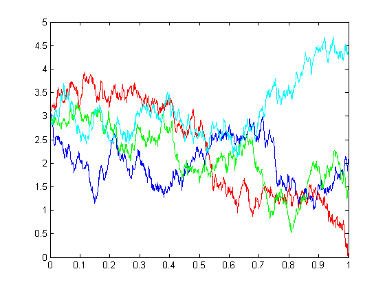
Figure 1. Four trajectories of the Wiener process with drift when $x_{0}=3,\mu=-1,\sigma=2.$

The programm in MatLab giving a simulation of four trajectories of the Wiener process with drift with parameters $\mu=-1$, $\sigma=3$, $x_{0}=3$ has the following form:

$x1=\mbox{random}(^{\prime}\mbox{Normal}^{\prime},0,1,4,1001);$

$m=-1;$

$s=2;$

$x0=3;$

$x=0:0.0001:1;$

$Y10=x0+m*x;$

$Y11=x1(1,1)*x;$

$Y20=x0+m*x;$

$Y21=x1(2,1)*x;$

$Y30=x0+m*x;$

$Y31=x1(3,1)*x;$

$Y40=x0+m*x;$

$Y41=x1(4,1)*x;$

$\mbox{for}~{}k=1:1000$

$Y11=Y11+\mbox{sqrt}(2)*x1(1,k+1)*sin(pi*k*x)/(pi*k);$

$Y21=Y21+\mbox{sqrt}(2)*x1(2,k+1)*sin(pi*k*x)/(pi*k);$

$Y31=Y31+\mbox{sqrt}(2)*x1(3,k+1)*sin(pi*k*x)/(pi*k);$

$Y41=Y41+\mbox{sqrt}(2)*x1(4,k+1)*sin(pi*k*x)/(pi*k);$

end

$X1=x;$

$Y1=Y10+s*Y11;$

$X2=x;$

$Y2=Y20+s*Y21;$

$X3=x;$

$Y3=Y30+s*Y31;$

$X4=x;$

$Y4=Y40+s*Y41;$

$\mbox{plot}(X1,Y1,^{\prime}b^{\prime},X2,Y2,^{\prime}r-^{\prime},X3,Y3,^{\prime}g^{\prime},X4,Y4,^{\prime}c^{\prime},^{\prime}\mbox{LineWidth}^{\prime},1)$

Below we present some numerical results obtaining by using MatLab and Microsoft Excel. In our simulation

(i)  $n$ denotes the number of trials;

(ii) $x_{0}=3$ is an initial position of the particle suspended in water;

(iii) $\mu=-1$ is the equilibrium or mean position supported by fundamentals;

(iv) $\sigma=2$ is the parameter of bombardment in Wiener process with drift ;

(v) $t=0.5$ is the moment of the observation on the Wiener process with drift ;

(vi) $z_{k}$ is the value of the $k$-th trajectory of Wiener process with drift at moment $t=0.5$ (see, Figure 1 and Table 4.1).

Table 4.1. The value $z_{k}$ of the the Wiener process with drift at moment $t=0.5$ when $x_{0}=3,\mu=-1,\sigma=2$.

$k$	$z_{k}$	$k$	$z_{k}$	$k$	$z_{k}$	$k$	$z_{k}$	$k$	$z_{k}$
$1$	$4.0991$	$21$	$2.7068$	$41$	$4.3571$	$61$	$3.5272$	$81$	$7.0549$
$2$	$1.6842$	$22$	$2.243$	$42$	$3.2793$	$62$	$2.8292$	$82$	$2.5627$
$3$	$2.9422$	$23$	$3.5946$	$43$	$3.2422$	$63$	$1.8519$	$83$	$1.5592$
$4$	$4.5744$	$24$	$4.6402$	$44$	$2.7395$	$64$	$-0.5223$	$84$	$3.8465$
$5$	$2.0157$	$25$	$2.2703$	$45$	$0.682$	$65$	$0.7602$	$85$	$0.8471$
$6$	$2.8821$	$26$	$2.681$	$46$	$3.4298$	$66$	$4.3529$	$86$	$2.8475$
$7$	$4.6284$	$27$	$2.9075$	$47$	$2.6592$	$67$	$1.1265$	$87$	$0.5144$
$8$	$1.654$	$28$	$3.3659$	$48$	$3.2093$	$68$	$1.3525$	$88$	$2.3558$
$9$	$0.9561$	$29$	$4.5149$	$49$	$0.1074$	$69$	$3.7889$	$89$	$2.4793$
$10$	$-0.5407$	$30$	$-1.3528$	$50$	$1.5462$	$70$	$3.2284$	$90$	$2.0639$
$11$	$1.98941$	$31$	$3.4294$	$51$	$1.0896$	$71$	$1.1392$	$91$	$1.166$
$12$	$4.3462$	$32$	$4.0825$	$52$	$2.1108$	$72$	$2.8833$	$92$	$3.2738$
$13$	$3.455$	$33$	$2.3837$	$53$	$2.9175$	$73$	$2.3093$	$93$	$0.4878$
$14$	$3.2235$	$34$	$3.3037$	$54$	$2.9352$	$74$	$1.4444$	$94$	$2.9504$
$15$	$2.1299$	$35$	$4.7552$	$55$	$3.5531$	$75$	$-0.23$	$95$	$2.4767$
$16$	$1.7554$	$36$	$2.1509$	$56$	$2.2376$	$76$	$1.1718$	$96$	$3.6022$
$17$	$3.9263$	$37$	$4.3749$	$57$	$1.6557$	$77$	$1.3588$	$97$	$1.6005$
$18$	$2.4328$	$38$	$2.6403$	$58$	$2.0076$	$78$	$1.5024$	$98$	$3.5125$
$19$	$2.9972$	$39$	$1.4087$	$59$	$0.8997$	$79$	$2.2622$	$99$	$2.2026$
$20$	$2.59$	$40$	$4.178$	$60$	$0.1873$	$80$	$3.3423$	$100$	$3.3646$

Table 4.2. The value of the statistic $T_{n}$ for the sample $(z_{k})_{1\leq k\leq n}(n=5i:1\leq i\leq 20)$ from the Table 4.1.

$n$	$T_{n}$	$\sigma^{2}$	$n$	$T_{n}$	$\sigma^{2}$
$5$	$3.182349256$	$4$	$55$	$3.463530492$	$4$
$10$	$4.995431962$	$4$	$60$	$3.472692797$	$4$
$15$	$4.029170383$	$4$	$65$	$3.628477887$	$4$
$20$	$3.30673624$	$4$	$70$	$3.621538801$	$4$
$25$	$3.120603594$	$4$	$75$	$3.662829637$	$4$
$30$	$3.924002323$	$4$	$80$	$3.554594699$	$4$
$35$	$3.884200678$	$4$	$85$	$3.96153126$	$4$
$40$	$3.781846824$	$4$	$90$	$3.836441056$	$4$
$45$	$3.715840465$	$4$	$95$	$3.774116249$	$4$
$50$	$3.665346353$	$4$	$100$	$3.663112062$	$4$

Remark 4.1 By use results of calculations placed in the Table 4.2, we see that the consistent estimator $T_{n}$ works successfully.

Table 4.3. The value of the statistic $T^{*}_{n}$ for the sample $(z_{k})_{1\leq k\leq n}(n=5i:1\leq i\leq 20)$ from the Table 4.1.

$n$	$T^{*}_{n}$	$\mu$	$n$	$T^{*}_{n}$	$\mu$
$5$	$0.12624$	$-1$	$55$	$-0.47716$	$-1$
$10$	$-1.0209$	$-1$	$60$	$-0.704466667$	$-1$
$15$	$-0.6614$	$-1$	$65$	$-0.851932308$	$-1$
$20$	$-0.62588$	$-1$	$70$	$-0.82396$	$-1$
$25$	$-0.464312$	$-1$	$75$	$-0.967797333$	$-1$
$30$	$-0.57916$	$-1$	$80$	$-1.0413725$	$-1$
$35$	$-0.327594286$	$-1$	$85$	$-0.959635294$	$-1$
$40$	$-0.299005$	$-1$	$90$	$-1.011635556$	$-1$
$45$	$-0.296888889$	$-1$	$95$	$-1.056187368$	$-1$
$50$	$-0.429124$	$-1$	$100$	$-1.01773$	$-1$

Remark 4.2 By use results of calculations placed in the Table 4.2, we see that the consistent estimator $T^{*}_{n}$ has a tendetion will come nearer to $\mu=-1$ as soon as the number of trials increases.

The following program gives animation of the Wiener process with drift over the time interval $[0,1]$ when $x_{0}=3,\mu=-1,\sigma=2$.

$N=100;$

$x1=\mbox{random}(^{\prime}\mbox{Normal}^{\prime},0,1,N,10001);$

$m=-1;$

$s=2;$

$x0=3;$

$x=0:0.0001:1;$

$Y0=x0+m*x;$

$Y1=x1(1)*x;$

$\mbox{for}~{}s=1:N$

$\mbox{for}~{}k=1:1000$

$Y1=Y1+sqrt(2)*x1(s,k+1)*sin(pi*k*x)/(pi*k);$

end

$X=x;$

$Y=Y0+s*Y1;$

$\mbox{plot}~{}(X,Y,^{\prime}r^{\prime},^{\prime}\mbox{LineWidth}^{\prime},1)$

$\mbox{drawnow};$

$\mbox{pause}(1);$

end

An animation given by this programm applies $N$ different trajectories which are defined by $N$ coppies of realizations of the finite family of independent standard Gaussian random variables of lenght $1001$ generated by Matlab operator $x1=random(^{\prime}Normal^{\prime},0,1,N,10001);$

5. Further investigations

Suppose that $(z^{(1)}_{k})_{k\in N}$ and $(z^{(2)}_{k})_{k\in N}$ are results of observations on the $2k$-th and $2k+1$-th trajectories of the Wiener process with drift at moments $t_{1}$ and $t_{2},$ respectively. Note that having such an information we can estimate unknown parameters $x_{0},\mu,\sigma$ for Wiener process with drift .

The first step in this direction is made by the following proposition.

Theorem 5.1  For $t>0$, $x_{0}\in R$, $\mu\in R$ and $\sigma>0$, let’s $\gamma_{(t,x_{0},\mu,\sigma)}$ be a Gaussian probability measure in $R$ with the mean $m_{t}=x_{0}+\mu t$ and the variance $\sigma_{t}^{2}=\sigma^{2}t$. Assuming that the parameter $\sigma$ is fixed, for $t_{1}>0$, $t_{2}>0$,$x_{0}\in R$, $\mu\in R$ denote by $\gamma_{(x_{0},\mu,t_{1})}$ and $\gamma_{(x_{0},\mu,t_{2})}$the measure $\gamma_{(t_{1},x_{0},\mu,\sigma)}$ and $\gamma_{(t_{2},x_{0},\mu,\sigma)}$, restectively.

We put $\gamma_{(x_{0},\mu)}=\gamma_{(x_{0},\mu,t_{1})}\times\gamma_{(x_{0},\mu,t_{2})}$. Let define the estimate ${\bf T}_{n}:(R^{2})^{n}\to R^{2}$ by the following formula

$(5.1)$ $${\bf T}_{n}((z^{(1)}_{k},z^{(2)}_{k})_{1\leq k\leq n})=(\frac{\sum_{k=1}^{n}(t_{2}z^{(1)}_{k}-t_{1}z^{(2)}_{k})}{n(t_{2}-t_{1})},\frac{\sum_{k=1}^{n}(z^{(2)}_{k}-z^{(1)}_{k})}{n(t_{2}-t_{1})}).$$

Then we get

$$\gamma_{(x_{0},\mu)}^{\infty}\{(z^{(1)}_{k},z^{(2)}_{k})_{k\in N}:(z^{(1)}_{k},z^{(2)}_{k})_{k\in N}\in(R^{2})^{\infty}$$

$(5.2)$ $$~{}\&~{}\lim_{n\to\infty}{\bf T}_{n}(((z^{(1)}_{k},(z^{(2)}_{k})_{1\leq k\leq n})=(x_{0},\mu)\}=1,$$

for $(x_{0},\mu)\in R^{2}$ provided that ${\bf T_{n}}$ is a consistent estimator of a parameter $(x_{0},\mu)$ for the family of probability measures $(\gamma_{(x_{0},\mu)}^{\infty})_{(x_{0},\mu)\in R^{2}}$.

Proof.

Let’s consider probability space $(\Omega,\mathcal{F},P)$, where $\Omega=(R^{2})^{\infty}$, $\mathcal{F}=B((R^{2})^{\infty})$, $P=\gamma_{(x_{0},\mu)}^{\infty}$.

For $k\in N$ we consider $k$-th projection ${\bf Pr}_{k}=(Pr^{(1)}_{k},Pr^{(2)}_{k})$ defined on $(R^{2})^{\infty}$ by

$(5.3)$ $${\bf Pr}_{k}((x^{(1)}_{i},x^{(2)}_{i})_{i\in N})=(x^{(1)}_{k},x^{(2)}_{k})$$

for $(x^{(1)}_{i},x^{(2)}_{i})_{i\in N}\in(R^{2})^{\infty}$.

It is obvious that $Pr^{(1)}_{k}((x^{(1)}_{i},x^{(2)}_{i})_{i\in N})=x^{(1)}_{k}$ and $Pr^{(2)}_{k}((x^{(1)}_{i},x^{(2)}_{i})_{i\in N})=x^{(2)}_{k}$ are also projection operators for $(x^{(1)}_{i},x^{(2)}_{i})_{i\in N}\in(R^{2})^{\infty}$.

It is obvious that $(Pr^{(1)}_{k})_{k\in N}$ is sequence of independent one-dimensional Gaussian random variables with expectaion equal to $x_{0}+\mu t_{1}$ and the variance equal to $\sigma^{2}t_{1}$. Similarly, $(Pr^{(2)}_{k})_{k\in N}$ is sequence of independent one-dimensional Gaussian random variables with expectaion equal to $x_{0}+\mu t_{2}$ and the variance equal to $\sigma^{2}t_{2}$.

Note that by use Kolmgorov strong law of large numbers, we have

$(5.4)$ $$\gamma_{(x_{0},\mu,t_{1})}^{\infty}(\{(z^{(1)}_{k})_{k\in N}:(z^{(1)}_{k})_{k\in N}\in R^{\infty}~{}\&~{}\lim_{n\to\infty}\frac{\sum_{k=1}^{n}z^{(1)}_{k}}{n}=x_{0}+\mu t_{1}\})=1$$

and

$(5.5)$ $$\gamma_{(x_{0},\mu,t_{2})}^{\infty}(\{(z^{(2)}_{k})_{k\in N}:(z^{(2)}_{k})_{k\in N}\in R^{\infty}~{}\&~{}\lim_{n\to\infty}\frac{\sum_{k=1}^{n}z^{(2)}_{k}}{n}=\mu+\mu t_{2}\})=1$$

We have

$$\gamma_{(x_{0},\mu)}^{\infty}\{(z^{(1)}_{k},z^{(2)}_{k})_{k\in N}:(z^{(1)}_{k},z^{(2)}_{k})_{k\in N}\in(R^{2})^{\infty}$$

$(5.6)$ $$~{}\&~{}\lim_{n\to\infty}{\bf T}_{n}((z^{(1)}_{k},z^{(2)}_{k})_{1\leq k\leq n})=(x_{0},\mu)\}$$

$$=\gamma_{(x_{0},\mu)}^{\infty}\{(z^{(1)}_{k},z^{(2)}_{k})_{k\in N}:(z^{(1)}_{k},z^{(2)}_{k})_{k\in N}\in(R^{2})^{\infty}$$

$$~{}\&~{}\lim_{n\to\infty}T^{(1)}_{n}(((z^{(1)}_{k},z^{(2)}_{k})_{1\leq k\leq n}=x_{0}~{}\&\lim_{n\to\infty}T^{(2)}_{n}(((z^{(1)}_{k},z^{(2)}_{k})_{1\leq k\leq n}=\mu\}$$

$$=\gamma_{(x_{0},\mu)}^{\infty}\{(z^{(1)}_{k},z^{(2)}_{k})_{k\in N}:(z^{(1)}_{k},z^{(2)}_{k})_{k\in N}\in(R^{2})^{\infty}$$

$$~{}\&~{}\lim_{n\to\infty}\frac{\sum_{k=1}^{n}(t_{2}z^{(1)}_{k}-t_{1}z^{(2)}_{k})}{n(t_{2}-t_{1})}=x_{0}~{}\&\lim_{n\to\infty}\frac{\sum_{k=1}^{n}(z^{(2)}_{k}-z^{(1)}_{k})}{n(t_{2}-t_{1})}=\mu\}$$

$$=\gamma_{(x_{0},\mu)}^{\infty}\{(z^{(1)}_{k},(z^{(2)}_{k})_{k\in N}:(z^{(1)}_{k},(z^{(2)}_{k})_{k\in N}\in(R^{2})^{\infty}$$

$$~{}\&~{}\lim_{n\to\infty}\frac{\sum_{k=1}^{n}z^{(1)}_{k}}{n}=x_{0}~{}\&\lim_{n\to\infty}\frac{\sum_{k=1}^{n}z^{(2)}_{k}}{n}=\mu\}$$

$$=\gamma_{(x_{0},\mu,t_{1})}^{\infty}(\{(z^{(1)}_{k})_{k\in N}:(z^{(1)}_{k})_{k\in N}\in(R)^{\infty}~{}\&~{}\lim_{n\to\infty}\frac{\sum_{k=1}^{n}z^{(1)}_{k}}{n}=x_{0}+\mu t_{1}\})$$

$$\times\gamma_{(x_{0},\mu,t_{2})}^{\infty}(\{(z^{(2)}_{k})_{k\in N}:(z^{(2)}_{k})_{k\in N}\in(R)^{\infty}~{}\&~{}\lim_{n\to\infty}\frac{\sum_{k=1}^{n}z^{(2)}_{k}}{n}=\mu+\mu t_{2}\})$$

(By use (5.4)-(5.5), we have )

$$=1\times 1=1.$$

∎

Theorem 5.2 Suppose that the family of probability measures $(\gamma_{(x_{0},\mu)}^{\infty})_{(x_{0},\mu)\in R^{2}}$ and the estimators ${\bf T}_{n}:(R^{2})^{n}\to R^{2}$ come from Theorem 5.1. Then the estimators ${\bf T}^{(0)}:R^{\infty}\to R$ and ${\bf T}^{(1)}:R^{\infty}\to R$ defined by

$(5.7)$ $${\bf T}^{(0)}((z^{(1)}_{k},z^{(2)}_{k})_{k\in N})=\underline{\lim}_{n\to\infty}{\bf T}_{n}((z^{(1)}_{k},z^{(2)}_{k})_{1\leq k\leq n})$$

and

$(5.8)$ $${\bf T}^{(0)}((z^{(1)}_{k},z^{(2)}_{k})_{k\in N})=\overline{\lim}_{n\to\infty}{\bf T}_{n}((z^{(1)}_{k},z^{(2)}_{k})_{1\leq k\leq n}).$$

are infinite-sample consistent estimators of a parameter $(x_{0},\mu)$ for the family of probability measures $(\gamma_{(x_{0},\mu)}^{\infty})_{(x_{0},\mu)\in R^{2}}$ .

Proof.

By using (5.2), we get

$$\gamma_{(x_{0},\mu)}^{\infty}\{z^{(1)}_{k},z^{(2)}_{k})_{k\in N}\in(R^{2})^{\infty}~{}\&~{}{\bf T}^{(0)}((z^{(1)}_{k},z^{(2)}_{k})_{k\in N})=(x_{0},\mu)\}$$

$$=\gamma_{(x_{0},\mu)}^{\infty}\{z^{(1)}_{k},z^{(2)}_{k})_{k\in N}\in(R^{2})^{\infty}~{}\&~{}\underline{\lim}_{n\to\infty}{\bf T}_{n}((z^{(1)}_{k},z^{(2)}_{k})_{1\leq k\leq n})=(x_{0},\mu)\}$$

$$\geq\gamma_{(x_{0},\mu)}^{\infty}\{z^{(1)}_{k},z^{(2)}_{k})_{k\in N}\in(R^{2})^{\infty}~{}\&~{}\lim_{n\to\infty}{\bf T}_{n}((z^{(1)}_{k},z^{(2)}_{k})_{1\leq k\leq n})=(x_{0},\mu)\}=1,$$

which means that ${\bf T}^{(0)}$ is an infinite-sample consistent estimators of a parameter $(x_{0},\mu)$ for the family of probability measures $(\gamma_{(x_{0},\mu)}^{\infty})_{(x_{0},\mu)\in R^{2}}$ .

Similarly, by using (5.2), we have

$$\gamma_{(x_{0},\mu)}^{\infty}\{z^{(1)}_{k},z^{(2)}_{k})_{k\in N}\in(R^{2})^{\infty}~{}\&~{}{\bf T}^{(1)}((z^{(1)}_{k},z^{(2)}_{k})_{k\in N})=(x_{0},\mu)\}$$

$$=\gamma_{(x_{0},\mu)}^{\infty}\{z^{(1)}_{k},z^{(2)}_{k})_{k\in N}\in(R^{2})^{\infty}~{}\&~{}\overline{\lim}_{n\to\infty}{\bf T}_{n}((z^{(1)}_{k},z^{(2)}_{k})_{1\leq k\leq n})=(x_{0},\mu)\}$$

$$\geq\gamma_{(x_{0},\mu)}^{\infty}\{z^{(1)}_{k},z^{(2)}_{k})_{k\in N}\in(R^{2})^{\infty}~{}\&~{}\lim_{n\to\infty}{\bf T}_{n}((z^{(1)}_{k},z^{(2)}_{k})_{1\leq k\leq n})=(x_{0},\mu)\}=1,$$

which means that ${\bf T}^{(1)}$ is also an infinite-sample consistent estimators of a parameter $(x_{0},\mu)$ for the family of probability measures $(\gamma_{(x_{0},\mu)}^{\infty})_{(x_{0},\mu)\in R^{2}}$ .

∎

Remark 5.1 Following Theorems 5.1-5.2, by using the values $(z^{(1)}_{k})_{k\in N}$ and $(z^{(2)}_{k})_{k\in N}$ being the results of observations on the $2k$-th and $2k+1$-th trajectories of the Wiener process with drift at moments $t_{1}$ and $t_{2}$ , respectively, we can estimate parameters $x_{0}$ and $\mu$. So an estimation of the parameter $\sigma$ is reduced to the case described in Theorem 3.1.

References

• [1] Bachar, Mostafa, Jerry J. Batzel, and Susanne Ditlevsen, eds. Stochastic biomathematical models: with applications to neuronal modeling. Vol. 2058. Springer, 2012.
• [2] Labadze L., Pantsulaia G., Estimation of the parameters of the Ornstein-Uhlenbeck’s stochastic process, http://arxiv.org/pdf/1608.04507v2.pdf
• [3] Shiryaev, A.N. 1980. Probability (in Russian), Izd.“Nauka”, Moscow.
• [4] Ibramkhallilov, I.Sh., Skorokhod, A.V. 1980. On well–off estimates of parameters of stochastic processes (in Russian), Kiev.
• [5] Stanoyevitch A., Introduction to MATLAB ® with numerical preliminaries. Wiley-Interscience, John Wiley $\&$ Sons, Hoboken, NJ, 2005.