General and Fractional Hypertree Decompositions:
Hard and Easy Cases

Abstract.

Hypertree decompositions, as well as the more powerful generalized hypertree decompositions (GHDs), and the yet more general fractional hypertree decompositions (FHD) are hypergraph decomposition methods successfully used for answering conjunctive queries and for solving constraint satisfaction problems. Every hypergraph $H$ has a width relative to each of these methods: its hypertree width $\mathit{hw}(H)$, its generalized hypertree width $\mathit{ghw}(H)$, and its fractional hypertree width $\mathit{fhw}(H)$, respectively. It is known that $\mathit{hw}(H)\leq k$ can be checked in polynomial time for fixed $k$, while checking $\mathit{ghw}(H)\leq k$ is NP-complete for $k\geq 3$. The complexity of checking $\mathit{fhw}(H)\leq k$ for a fixed $k$ has been open for over a decade.

We settle this open problem by showing that checking $\mathit{fhw}(H)\leq k$ is NP-complete, even for $k=2$. The same construction allows us to prove also the NP-completeness of checking $\mathit{ghw}(H)\leq k$ for $k=2$. After that, we identify meaningful restrictions which make checking for bounded $\mathit{ghw}$ or $\mathit{fhw}$ tractable or allow for an efficient approximation of the $\mathit{fhw}$.

1. Introduction and Background

Research Challenges Tackled. In this work we tackle computational problems on hypergraph decompositions, which play a prominent role for answering Conjunctive Queries (CQs) and solving Constraint Satisfaction Problems (CSPs), which we discuss below.

Many NP-hard graph-based problems become tractable for instances whose corresponding graphs have bounded treewidth. There are, however, many problems for which the structure of an instance is better described by a hypergraph than by a graph, for example, the above mentioned CQs and CSPs. Given that treewidth does not generalize hypergraph acyclicity, proper hypergraph decomposition methods have been developed, in particular, hypertree decompositions (HDs) (Gottlob et al., 2002), the more general generalized hypertree decompositions (GHDs) (Gottlob et al., 2002), and the yet more general fractional hypertree decompositions (FHDs) (Grohe and Marx, 2014), and corresponding notions of width of a hypergraph $H$ have been defined: the hypertree width $\mathit{hw}(H)$, the generalized hypertree width $\mathit{ghw}(H)$, and the fractional hypertree width $\mathit{fhw}(H)$, where for every hypergraph $H$, $\mathit{fhw}(H)\leq\mathit{ghw}(H)\leq\mathit{hw}(H)$ holds. Definitions are given in Section 2. A number of highly relevant hypergraph-based problems such as CQ-evaluation and CSP-solving become tractable for classes of instances of bounded $\mathit{hw}$, $\mathit{ghw}$, or, $\mathit{fhw}$. For each of the mentioned types of decompositions it would thus be useful to be able to recognize for each constant $k$ whether a given hypergraph $H$ has corresponding width at most $k$, and if so, to compute such a decomposition. More formally, for decomposition $\in\{$HD, GHD, FHD$\}$ and $k>0$, we consider the following family of problems:

Check(decomposition, $k$)
input hypergraph $H=(V,E)$; output decomposition of $H$ of width $\leq k$ if it exists and answer ‘no’ otherwise.

As shown in (Gottlob et al., 2002), Check(HD, $k$)  is in Ptime. However, little is known about Check(FHD, $k$). In fact, this has been an open problem since the 2006 paper (Grohe and Marx, 2006), where Grohe and Marx state: “It remains an important open question whether there is a polynomial-time algorithm that determines (or approximates) the fractional hypertree width and constructs a corresponding decomposition.” The 2014 journal version still mentions this as open and it is conjectured that the problem might be NP-hard. The open problem is restated in (van Bevern et al., 2015), where further evidence for the hardness of the problem is given by showing that “it is not expressible in monadic second-order logic whether a hypergraph has bounded (fractional, generalized) hypertree width”. We will tackle this open problem here:

• Research Challenge 1:  Is Check(FHD, $k$) tractable?

Let us now turn to generalized hypertree decompositions. In (Gottlob et al., 2002) the complexity of Check(GHD, $k$) was stated as an open problem. In (Gottlob et al., 2009), it was shown that Check(GHD, $k$) is NP-complete for $k\geq 3$. For $k=1$ the problem is trivially tractable because $\mathit{ghw}(H)=1$ just means $H$ is acyclic. However the case $k=2$ has been left open. This case is quite interesting, because it was observed that the majority of practical queries from various benchmarks that are not acyclic have $\mathit{ghw}=2$ (Bonifati et al., 2017; Fischl et al., 2019), and that a decomposition in such cases can be very helpful. Our second research goal is to finally settle the complexity of Check(GHD, $k$) completely.

• Research Challenge 2:  Is Check(GHD, $2$) tractable?

For those problems which are known to be intractable, for example, Check(GHD, $k$) for $k\geq 3$, and for those others that will turn out to be intractable, we would like to find large islands of tractability that correspond to meaningful restrictions of the input hypergraph instances. Ideally, such restrictions should fulfil two main criteria: (i) they need to be realistic in the sense that they apply to a large number of CQs and/or CSPs in real-life applications, and (ii) they need to be non-trivial in the sense that the restriction itself does not already imply bounded $\mathit{hw}$, $\mathit{ghw}$, or $\mathit{fhw}$. Trivial restrictions would be, for example, acyclicity or bounded treewidth. Hence, our third research problem is as follows:

• Research Challenge 3:  Find realistic, non-trivial restrictions on hypergraphs which entail the tractability of the Check(decomp, $k$) problem for decomp $\in\{$GHD, FHD$\}$.

Where we do not achieve Ptime algorithms for the precise computation of a decomposition of optimal width, we would like to find tractable methods for achieving good approximations. Note that for GHDs, the problem of approximations is solved, since $\mathit{ghw}(H)\leq 3\cdot\mathit{hw}(H)+1$ holds for every hypergraph $H$ (Adler et al., 2007). In contrast, for FHDs, the best known polynomial-time approximation is cubic. More precisely, in (Marx, 2010), a polynomial-time algorithm is presented which, given a hypergraph $H$ with $\mathit{fhw}(H)=k$, computes an FHD of width ${\mathcal{O}}(k^{3})$. We would like to find meaningful restrictions that guarantee significantly tighter approximations in polynomial time. This leads to the fourth research problem:

• Research Challenge 4:  Find realistic, non-trivial restrictions on hypergraphs which allow us to compute in Ptime good approximations of $\mathit{fhw}(k)$.

Background and Applications. Hypergraph decompositions have meanwhile found their way into commercial database systems such as LogicBlox (Aref et al., 2015; Olteanu and Závodný, 2015; Bakibayev et al., 2013; Khamis et al., 2015, 2016) and advanced research prototypes such as EmptyHeaded (Aberger et al., 2016a; Tu and Ré, 2015; Aberger et al., 2016b). Moreover, since CQs and CSPs of bounded hypertree width fall into the highly parallelizable complexity class LogCFL, hypergraph decompositions have also been discovered as a useful tool for parallel query processing with MapReduce (Afrati et al., 2017). Hypergraph decompositions, in particular, HDs and GHDs have been used in many other contexts, e.g., in combinatorial auctions (Gottlob and Greco, 2013) and automated selection of Web services based on recommendations from social networks (Hashmi et al., 2016). There exist exact algorithms for computing the generalized or fractional hypertree width (Moll et al., 2012); clearly, they require exponential time even if the optimal width is bounded by some fixed $k$.

CQs are the most basic and arguably the most important class of queries in the database world. Likewise, CSPs constitute one of the most fundamental classes of problems in Artificial Intelligence. Formally, CQs and CSPs are the same problem and correspond to first-order formulae using $\{\exists,\wedge\}$ but disallowing $\{\forall,\vee,\neg\}$ as connectives, that need to be evaluated over a set of finite relations: the database relations for CQs, and the constraint relations for CSPs. In practice, CQs have often fewer conjuncts (query atoms) and larger relations, while CSPs have more conjuncts but smaller relations. These problems are well-known to be NP-complete (Chandra and Merlin, 1977). Consequently, there has been an intensive search for tractable fragments of CQs and/or CSPs over the past decades. For our work, the approaches based on decomposing the structure of a given CQ or CSP are most relevant, see e.g. (Gyssens and Paredaens, 1984; Dechter and Pearl, 1989; Freuder, 1990; Gyssens et al., 1994; Kolaitis and Vardi, 2000; Grohe et al., 2001; Dalmau et al., 2002; Chekuri and Rajaraman, 2000; Gottlob et al., 2002; Chen and Dalmau, 2005; Grohe, 2007; Cohen et al., 2008; Marx, 2011, 2013; Atserias et al., 2013; Grohe and Marx, 2014). The underlying structure of both is nicely captured by hypergraphs. The hypergraph $H=(V(H),E(H))$ underlying a CQ (or a CSP) $Q$ has as vertex set $V(H)$ the set of variables occurring in $Q$; moreover, for every atom in $Q$, $E(H)$ contains a hyperedge consisting of all variables occurring in this atom. From now on, we shall mainly talk about hypergraphs with the understanding that all our results are equally applicable to CQs and CSPs.

Main Results. First of all, we have investigated the above mentioned open problem concerning the recognizability of $\mathit{fhw}\leq k$ for fixed $k$. Our initial hope was to find a simple adaptation of the NP-hardness proof in (Gottlob et al., 2009) for recognizing $\mathit{ghw}(H)\leq k$, for $k\geq 3$. Unfortunately, this proof dramatically fails for the fractional case. In fact, the hypergraph-gadgets in that proof are such that both “yes” and “no” instances may yield the same $\mathit{fhw}$. However, via crucial modifications, including the introduction of novel gadgets, we succeed to construct a reduction from 3SAT that allows us to control the $\mathit{fhw}$ of the resulting hypergraphs such that those hypergraphs arising from “yes” 3SAT instances have $\mathit{fhw}(H)=2$ and those arising from “no” instances have $\mathit{fhw}(H)>2$. Surprisingly, thanks to our new gadgets, the resulting proof is actually significantly simpler than the NP-hardness proof for recognizing $\mathit{ghw}(H)\leq k$ in (Gottlob et al., 2009). We thus obtain the following result:

• Main Result 1: Deciding $\mathit{fhw}(H)\leq 2$ for hypergraphs $H$ is NP-complete and, therefore, Check(FHD, $k$) is intractable even for $k=2$.

This result can be extended to the NP-hardness of recognizing $\mathit{fhw}(H)\leq k$ for arbitrarily large $k$. Moreover, the same construction can be used to prove that recognizing ghw $\leq 2$ is also NP-hard, thus killing two birds with one stone.

• Main Result 2: Deciding $\mathit{ghw}(H)\leq 2$ for hypergraphs $H$ is NP-complete and, therefore, Check(GHD, $2$) is intractable even for $k=2$.

The Main Results 1 and 2 are presented in Section 3. These results close some smouldering open problems with bad news. We thus further concentrate on Research Challenges 3 and 4 in order to obtain some positive results for restricted hypergraph classes.

We first study GHDs, where we succeed to identify very general, realistic, and non-trivial restrictions that make the Check(GHD, $k$) problem tractable. These results are based on new insights about the differences of GHDs and HDs and the introduction of a novel technique for expanding a hypergraph $H$ to an edge-augmented hypergraph $H^{\prime}$ s.t. the width $k$ GHDs of $H$ correspond to the width $k$ HDs of $H^{\prime}$. The crux here is to find restrictions under which only a polynomial number of edges needs to be added to $H$ to obtain $H^{\prime}$. The HDs of $H^{\prime}$ can then be computed in polynomial time.

In particular, we concentrate on the bounded intersection property (BIP), which, for a class $\mathscr{C}$ of hypergraphs requires that for some constant $i$, for each pair of distinct edges $e_{1}$ and $e_{2}$ of each hypergraph $H\in{\mathscr{C}}$, $|e_{1}\cap e_{2}|\leq i$, and its generalization, the bounded multi-intersection property (BMIP), which, informally, requires that for some constant $c$ any intersection of $c$ distinct hyperedges of $H$ has at most $i$ elements for some constant $i$. In (Fischl et al., 2019) we report on tests with a large number of known CQ and CSP benchmarks and it turns out that a very large number of instances coming from real-life applications enjoy the BIP and a yet more overwhelming number enjoys the BMIP for very low constants $c$ and $i$. We obtain the following good news, which are presented in Section 4.

• Main Result 3: For classes of hypergraphs fulfilling the BIP or BMIP, for every constant $k$, the problem Check(GHD, $k$) is tractable. Tractability holds even for classes $\mathscr{C}$ of hypergraphs where for some constant $c$ all intersections of $c$ distinct edges of every $H\in{\mathscr{C}}$ of size $n$ have ${\mathcal{O}}(\log n)$ elements. Our complexity analysis reveals that the problem Check(GHD, $k$) is fixed-parameter tractable w.r.t. parameter $i$ of the BIP.

The tractability proofs for BIP and BMIP do not directly carry over to FHDs. We thus consider the degree $d$ of a hypergraph $H=(V(H),E(H))$, which is defined as the maximum number of hyperedges in which a vertex occurs, i.e., $d=\max_{v\in V(H)}|\{e\in E(H)\mid v\in E(H)\}|$. We say that a class $\mathscr{C}$ of hypergraphs has the bounded degree property (BDP), if there exists $d\geq 1$, such that every hypergraph $H\in{\mathscr{C}}$ has degree $\leq d$. We obtain the following result, which is presented in Section 5.

• Main Result 4: For classes of hypergraphs fulfilling the BDP and for every constant $k$, the problem Check(FHD, $k$) is tractable.

To get yet bigger tractable classes, we also consider approximations of an optimal FHD. Towards this goal, we study the $\mathit{fhw}$ in case of the BIP and we establish an interesting connection between the BMIP and the Vapnik–Chervonenkis dimension (VC-dimension) of hypergraphs. Our research, presented in Section 6 is summarized as follows.

• Main Result 5: For rather general, realistic, and non-trivial hypergraph restrictions, there exist Ptime algorithms that, for hypergraphs $H$ with $\mathit{fhw}(H)=k$, where $k$ is a constant, produce FHDs whose widths are significantly smaller than the best previously known approximation. In particular, the BIP allows us to compute in polynomial time an FHD whose width is $\leq k+\epsilon$ for arbitrarily chosen constant $\epsilon>0$. The BMIP or bounded VC-dimension allow us to compute in polynomial time an FHD whose width is ${\mathcal{O}}(k\log k)$.

We finally turn our attention also to the optimization problem of fractional hypertree width, i.e., given a hypergraph $H$, determine $\mathit{fhw}(H)$ and find an FHD of width $\mathit{fhw}(H)$. All our algorithms for the Check(FHD, $k$) problem have a runtime exponential in the desired width $k$. Hence, even with the restrictions to the BIP or BMIP we cannot expect an efficient approximation of $\mathit{fhw}$ if $\mathit{fhw}$ can become arbitrarily large. We will therefore study the following $K$-Bounded-FHW-Optimization problem for constant $K\geq 1$:

$K$-Bounded-FHW-Optimization
input hypergraph $H=(V,E)$; output if $\mathit{fhw}(H)\leq K$: find an FHD $\mathcal{F}$ of $H$ with minimum width; otherwise: answer “$\mathit{fhw}(H)>K$”.

For this bounded version of the optimization problem, we will prove the following result:

• Main Result 6: There exists a polynomial time approximation scheme (PTAS; for details see Section 6) for the $K$-Bounded-FHW-Optimization problem in case of the BIP for any fixed $K\geq 1$.

2. Preliminaries

2.1. Hypergraphs

A hypergraph is a pair $H=(V(H),E(H))$, consisting of a set $V(H)$ of vertices and a set $E(H)$ of hyperedges (or, simply edges), which are non-empty subsets of $V(H)$. We assume that hypergraphs do not have isolated vertices, i.e. for each $v\in V(H)$, there is at least one edge $e\in E(H)$, s.t. $v\in e$. For a set $C\subseteq V(H)$, we define $\mathit{edges}(C)=\{e\in E(H)\mid e\cap C\neq\emptyset\}$ and for a set $S\subseteq E(H)$, we define $\mathit{V}(S)=\{v\in e\mid e\in S\}$. Actually, for a set $S$ of edges, it is convenient to write $\bigcup S$ (and $\bigcap S$, respectively) to denote the set of vertices obtained by taking the union (or the intersection, respectively) of the edges in $E$. Hence, we can write $\mathit{V}(S)$ simply as $\bigcup S$.

For a hypergraph $H$ and a set $C\subseteq V(H)$, we say that a pair of vertices $v_{1},v_{2}\in V(H)$ is [$C$]-adjacent if there exists an edge $e\in E(H)$ such that $\{v_{1},v_{2}\}\subseteq(e\setminus C)$. A [$C$]-path $\pi$ from $v$ to $v^{\prime}$ consists of a sequence $v=v_{0},\dots,v_{h}=v^{\prime}$ of vertices and a sequence of edges $e_{0},\dots,e_{h-1}$ ($h\geq 0$) such that $\{v_{i},v_{i+1}\}\subseteq(e_{i}\setminus C)$, for each $i\in[0\ldots h-1]$. We denote by $\mathit{V}(\pi)$ the set of vertices occurring in the sequence $v_{0},\ldots,v_{h}$. Likewise, we denote by $\mathit{edges}(\pi)$ the set of edges occurring in the sequence $e_{0},\ldots,e_{h-1}$. A set $W\subseteq V(H)$ of vertices is [$C$]-connected if $\forall v,v^{\prime}\in W$ there is a [$C$]-path from $v$ to $v^{\prime}$. A [$C$]-component is a maximal [$C$]-connected, non-empty set of vertices $W\subseteq V(H)\setminus C$.

2.2. (Fractional) Edge Covers

Let $H=(V(H),E(H))$ be a hypergraph and consider (edge-weight) functions $\lambda\colon E(H)\rightarrow\{0,1\}$ and $\gamma\colon E(H)\rightarrow[0,1]$. For $\theta\in\{\lambda,\gamma\}$, we denote by $B(\theta)$ the set of all vertices covered by $\theta$:

$$B(\theta)=\left\{v\in V(H)\mid\sum_{e\in E(H),v\in e}\theta(e)\geq 1\right\}$$

The weight of such a function $\theta$ is defined as

$$\mathit{weight}(\theta)=\sum_{e\in E(H)}\theta(e).$$

Following (Gottlob et al., 2002), we will sometimes consider $\lambda$ as a set with $\lambda\subseteq E(H)$ (i.e., the set of edges $e$ with $\lambda(e)=1$) and the weight of $\lambda$ as the cardinality of this set. However, for the sake of a uniform treatment with function $\gamma$, we shall prefer to treat $\lambda$ as a function.

Definition 2.1.

An edge cover of a hypergraph $H$ is a function $\lambda:E(H)\rightarrow\{0,1\}$ such that $V(H)=B(\lambda)$. The edge cover number $\rho(H)$ is the minimum weight of all edge covers of $H$.

Note that the edge cover number can be calculated by the following integer linear program (ILP).

minimize: $$\sum_{e\in E(H)}\lambda(e)$$

subject to: $$\quad\sum_{\mathclap{e\in E(H),v\in e}}\;\lambda(e)\geq 1, \text{for all }v\in V(H)$$

$$\lambda(e)\in\{0,1\} \text{for all }e\in E(H)$$

By substituting all $\lambda(e)$ by $\gamma(e)$ and by relaxing the last condition of the ILP above to $\gamma(e)\geq 0$, we arrive at the linear program (LP) for computing the fractional edge cover number to be defined next. Note that even though our weight function is defined to take values between 0 and 1, we do not need to add $\gamma(e)\leq 1$ as a constraint, because implicitly by the minimization itself the weight on an edge for an edge cover is never greater than 1. Also note that now the program above is an LP, which (in contrast to an ILP) can be solved in Ptime even if $k$ is not fixed.

Definition 2.2.

A fractional edge cover of a hypergraph $H=(V(H),E(H))$ is a function $\gamma:E(H)\rightarrow[0,1]$ such that $V(H)=B(\gamma)$. The fractional edge cover number $\rho^{*}(H)$ of $H$ is the minimum weight of all fractional edge covers of $H$. We write $\mathit{supp}(\gamma)$ to denote the support of $\gamma$, i.e., $\mathit{supp}(\gamma):=\{e\in E(H)\mid\gamma(e)>0\}$.

Clearly, we have $\rho^{*}(H)\leq\rho(H)$ for every hypergraph $H$, and $\rho^{*}(H)$ can be much smaller than $\rho(H)$. However, below we give an example, which is important for our proof of Theorem 3.2 and where $\rho^{*}(H)$ and $\rho(H)$ coincide.

Lemma 2.3.

Let $K_{2n}$ be a clique of size $2n$. Then the equalities $\rho(K_{2n})=\rho^{*}(K_{2n})=n$ hold.

Proof.

Since we have to cover each vertex with weight $\geq 1$, the total weight on the vertices of the graph is $\geq 2n$. As the weight of each edge adds to the weight of at most 2 vertices, we need at least weight $n$ on the edges to achieve $\geq 2n$ weight on the vertices. On the other hand, we can use $n$ edges each with weight 1 to cover $2n$ vertices. Hence, in total, we get $n\leq\rho^{*}(K_{2n})\leq\rho(K_{2n})\leq n$. ∎

2.3. HDs, GHDs, and FHDs

We now define three types of hypergraph decompositions:

Definition 2.4.

A generalized hypertree decomposition (GHD) of a hypergraph $H=(V(H),E(H))$ is a tuple $\left<T,(B_{u})_{u\in N(T)},(\lambda_{u})_{u\in N(T)}\right>$, such that $T=\left<N(T),E(T)\right>$ is a rooted tree and the following conditions hold:

1. for each $e\in E(H)$, there is a node $u\in N(T)$ with $e\subseteq B_{u}$;

2. for each $v\in V(H)$, the set $\{u\in N(T)\mid v\in B_{u}\}$ is connected in $T$;

3. for each $u\in N(T)$, $\lambda_{u}$ is a function $\lambda_{u}\colon E(H)\rightarrow\{0,1\}$ with $B_{u}\subseteq B(\lambda_{u})$.

Let us clarify some notational conventions used throughout this paper. To avoid confusion, we will consequently refer to the elements in $V(H)$ as vertices (of the hypergraph) and to the elements in $N(T)$ as the nodes of $T$ (of the decomposition). Now consider a decomposition $\mathcal{G}$ with tree structure $T$. For a node $u$ in $T$, we write $T_{u}$ to denote the subtree of $T$ rooted at $u$. By slight abuse of notation, we will often write $u^{\prime}\in T_{u}$ to denote that $u^{\prime}$ is a node in the subtree $T_{u}$ of $T$. Moreover, we define $V(T_{u}):=\bigcup_{u^{\prime}\in T_{u}}B_{u^{\prime}}$ and, for a set $V^{\prime}\subseteq V(H)$, we define $\mathit{nodes}(V^{\prime})=\{u\in T\mid B_{u}\cap V^{\prime}\neq\emptyset\}$. If we want to make explicit the decomposition $\mathcal{G}$, we also write $\mathit{nodes}(V^{\prime},\mathcal{G})$ synonymously with $\mathit{nodes}(V^{\prime})$. By further overloading the $\mathit{nodes}$ operator, we also write $\mathit{nodes}(T_{u})$ or $\mathit{nodes}(T_{u},\mathcal{G})$ to denote the nodes in a subtree $T_{u}$ of $T$, i.e., $\mathit{nodes}(T_{u})=\mathit{nodes}(T_{u},\mathcal{G})=\{v\mid v\in T_{u}\}$.

Definition 2.5.

A hypertree decomposition (HD) of a hypergraph $H=(V(H),E(H))$ is a GHD, which in addition also satisfies the following condition:

1. for each $u\in N(T)$, $V(T_{u})\cap B(\lambda_{u})\subseteq B_{u}$

Definition 2.6.

A fractional hypertree decomposition (FHD) (Grohe and Marx, 2014) of a hypergraph $H=(V(H),E(H))$ is a tuple $\left<T,(B_{u})_{u\in N(T)},(\gamma)_{u\in N(T)}\right>$, where conditions (1) and (2) of Definition 2.4 plus condition (3’) hold:

1. for each $u\in N(T)$, $\gamma_{u}$ is a function $\gamma_{u}:E(H)\rightarrow[0,1]$ with $B_{u}\subseteq B(\gamma_{u})$.

The width of a GHD, HD, or FHD is the maximum weight of the functions $\lambda_{u}$ or $\gamma_{u}$, respectively, over all nodes $u$ in $T$. Moreover, the generalized hypertree width, hypertree width, and fractional hypertree width of $H$ (denoted $\mathit{ghw}(H)$, $\mathit{hw}(H)$, $\mathit{fhw}(H)$) is the minimum width over all GHDs, HDs, and FHDs of $H$, respectively. Condition (2) is called the “connectedness condition”, and condition (4) is referred to as “special condition” (Gottlob et al., 2002). The set $B_{u}$ is often referred to as the “bag” at node $u$. Note that, strictly speaking, only HDs require that the underlying tree $T$ be rooted. For the sake of a uniform treatment we assume that also the tree underlying a GHD or an FHD is rooted (with the understanding that the root is arbitrarily chosen).

We now recall two fundamental properties of the various notions of decompositions and width.

Lemma 2.7.

Let $H$ be a hypergraph and let $H^{\prime}$ be a vertex induced subhypergraph of $H$, then $\mathit{hw}(H^{\prime})\leq\mathit{hw}(H)$, $\mathit{ghw}(H^{\prime})\leq\mathit{ghw}(H)$, and $\mathit{fhw}(H^{\prime})\leq\mathit{fhw}(H)$ hold.

Lemma 2.8.

Let $H$ be a hypergraph. If $H$ has a subhypergraph $H^{\prime}$ such that $H^{\prime}$ is a clique, then every HD, GHD, or FHD of $H$ has a node $u$ such that $V(H^{\prime})\subseteq B_{u}$.

Strictly speaking, Lemma 2.8 is a well-known property of tree decompositions – independently of the $\lambda$- or $\gamma$-label.

3. NP-Hardness

The main result in this section is the NP-hardness of Check(decomp, $k$) with decomp $\in\{$GHD, FHD$\}$ and $k=2$. At the core of the NP-hardness proof is the construction of a hypergraph $H$ with certain properties. The gadget in Figure 1 will play an integral part of this construction.

Figure 1. Basic structure of $H_{0}$ in Lemma 3.1

Lemma 3.1.

Let $M_{1}$, $M_{2}$ be disjoint sets and $M=M_{1}\cup M_{2}$. Let $H=(V(H),E(H))$ be a hypergraph and $H_{0}=$ $(V_{0},E_{A}\cup E_{B}\cup E_{C})$ a subhypergraph of $H$ with $V_{0}=\{a_{1},a_{2},b_{1},b_{2},c_{1},c_{2},d_{1},d_{2}\}\cup M$ and

$$E_{A}=\{ \{a_{1},b_{1}\}\cup M_{1},\{a_{2},b_{2}\}\cup M_{2},\{a_{1},b_{2}\},\{a_{2},b_{1}\},\{a_{1},a_{2}\}\}$$

$$E_{B}=\{ \{b_{1},c_{1}\}\cup M_{1},\{b_{2},c_{2}\}\cup M_{2},\{b_{1},c_{2}\},\{b_{2},c_{1}\},\{b_{1},b_{2}\},\{c_{1},c_{2}\}\}$$

$$E_{C}=\{ \{c_{1},d_{1}\}\cup M_{1},\{c_{2},d_{2}\}\cup M_{2},\{c_{1},d_{2}\},\{c_{2},d_{1}\},\{d_{1},d_{2}\}\}$$

where no element from the set $R=\{a_{2},b_{1},b_{2},c_{1},c_{2},d_{1},d_{2}\}$ occurs in any edge of $E(H)\setminus(E_{A}\cup E_{B}\cup E_{C})$. Then, every FHD $\mathcal{F}=\left<T,(B_{u})_{u\in T},(\gamma_{u})_{u\in T}\right>$ of width $\leq 2$ of H has nodes $u_{A},u_{B},u_{C}$ s.t.:

• $\{a_{1},a_{2},b_{1},b_{2}\}\subseteq B_{u_{A}}\subseteq M\cup\{a_{1},a_{2},b_{1},b_{2}\}$

• $B_{u_{B}}=\{b_{1},b_{2},c_{1},c_{2}\}\cup M$,

• $\{c_{1},c_{2},d_{1},d_{2}\}\subseteq B_{u_{C}}\subseteq M\cup\{c_{1},c_{2},d_{1},d_{2}\}$, and

• $u_{B}$ is on the path from $u_{A}$ to $u_{C}$.

Proof.

Consider an arbitrary FHD $\mathcal{F}=\left<T,(B_{u})_{u\in T},(\gamma_{u})_{u\in T}\right>$ of width $\leq 2$ of H. Observe that $a_{1},a_{2},b_{1}$, and $b_{2}$ form a clique of size 4. Hence, by Lemma 2.8, there is a node $u_{A}$ in $\mathcal{F}$, such that $\{a_{1},a_{2},b_{1},b_{2}\}\subseteq B_{u_{A}}$. It remains to show that also $B_{u_{A}}\subseteq M\cup\{a_{1},a_{2},b_{1},b_{2}\}$ holds. To this end, we use a similar reasoning as in the proof of Lemma 2.3: to cover each vertex in $\{a_{1},a_{2},b_{1},b_{2}\}$, we have to put weight $\geq 1$ on each of these 4 vertices. By assumption, the only edges containing 2 out of these 4 vertices are the edges in $E_{A}\cup\{\{b_{1},b_{2}\}\}$. All other edges in $E(H)$ contain at most 1 out of these 4 vertices. Hence, in order to cover $\{a_{1},a_{2},b_{1},b_{2}\}$ with weight $\leq 2$, we are only allowed to put non-zero weight on the edges in $E_{A}\cup\{\{b_{1},b_{2}\}\}$. It follows, that $B_{u_{A}}\subseteq M\cup\{a_{1},a_{2},b_{1},b_{2}\}$ indeed holds.

Analogously, for the cliques $b_{1},b_{2},c_{1},c_{2}$ and $c_{1},c_{2},d_{1},d_{2}$, there must exist nodes $u_{B}$ and $u_{C}$ in $\mathcal{F}$ with $\{b_{1},b_{2},c_{1},c_{2}\}\subseteq B_{u_{B}}\subseteq M\cup\{b_{1},b_{2},c_{1},c_{2}\}$ and $\{c_{1},c_{2},d_{1},d_{2}\}\subseteq B_{u_{C}}\subseteq M\cup\{c_{1},c_{2},d_{1},d_{2}\}$.

It remains to show that $u_{B}$ is on the path from $u_{A}$ to $u_{C}$ and $B_{u_{B}}=\{b_{1},b_{2},c_{1},c_{2}\}\cup M$ holds. We first show that $u_{B}$ is on the path between $u_{A}$ and $u_{C}$. Suppose to the contrary that it is not. We distinguish two cases. First, assume that $u_{A}$ is on the path between $u_{B}$ and $u_{C}$. Then, by connectedness, $\{c_{1},c_{2}\}\subseteq B_{u_{A}}$, which contradicts the property $B_{u_{A}}\subseteq M\cup\{a_{1},a_{2},b_{1},b_{2}\}$ shown above. Second, assume $u_{C}$ is on the path between $u_{A}$ and $u_{B}$. In this case, we have $\{b_{1},b_{2}\}\subseteq B_{u_{C}}$, which contradicts the property $B_{u_{C}}\subseteq M\cup\{c_{1},c_{2},d_{1},d_{2}\}$ shown above.

We now show that also $B_{u_{B}}=\{b_{1},b_{2},c_{1},c_{2}\}\cup M$ holds. Since we have already established $\{b_{1},b_{2},c_{1},c_{2}\}\subseteq B_{u_{B}}\subseteq M\cup\{b_{1},b_{2},c_{1},c_{2}\}$, it suffices to show $M\subseteq B_{u_{B}}$. First, let $T^{\prime}_{a}$ be the subgraph of $T$ induced by $\mathit{nodes}(\{a_{1},a_{2}\},\mathcal{F})$ and let $T^{\prime}_{d}$ be the subgraph of $T$ induced by $\mathit{nodes}(\{d_{1},d_{2}\},\mathcal{F})$. We show that each of the subgraphs $T^{\prime}_{a}$ and $T^{\prime}_{d}$ is connected (i.e., a subtree of $T$) and that the two subtrees are disjoint. The connectedness is immediate: by the connectedness condition, each of $\mathit{nodes}(\{a_{1}\},\mathcal{F})$, $\mathit{nodes}(\{a_{2}\},\mathcal{F})$, $\mathit{nodes}(\{d_{1}\},\mathcal{F})$, and $\mathit{nodes}(\{d_{2}\},\mathcal{F})$ is connected. Moreover, since $H$ contains an edge $\{a_{1},a_{2}\}$ (resp. $\{d_{1},d_{2}\}$), the two subtrees induced by $\mathit{nodes}(\{a_{1}\},\mathcal{F})$, $\mathit{nodes}(\{a_{2}\},\mathcal{F})$ (resp. $\mathit{nodes}(\{d_{1}\},\mathcal{F})$, $\mathit{nodes}(\{d_{2}\},\mathcal{F})$) must be connected, hence $T^{\prime}_{a}$ and $T^{\prime}_{d}$ are subtrees of $T$. It remains to show that $T^{\prime}_{a}$ and $T^{\prime}_{d}$ are disjoint.

Suppose to the contrary that there exists a node $u$ which is both in $T^{\prime}_{a}$ and in $T^{\prime}_{d}$, i.e., $a_{i},d_{j}\in B_{u}$ for some $i\in\{1,2\}$ and $j\in\{1,2\}$. We claim that $u$ must be on the path between $u_{A}$ and $u_{C}$. Suppose it is not. This means that either $u_{A}$ is on the path between $u$ and $u_{C}$ or $u_{C}$ is on the path between $u$ and $u_{A}$. In the first case, $B_{u_{A}}$ has to contain $d_{j}$ by the connectedness condition, which we have already ruled out above. In the second case, $B_{u_{C}}$ has to contain $a_{i}$, which we have also ruled out above. Hence, $u$ is indeed on the path between $u_{A}$ and $u_{C}$. We have already shown above that also $u_{B}$ is on the path between $u_{A}$ and $u_{C}$. Hence, there are two cases depending on how $u$ and $u_{B}$ are arranged on the path between $u_{A}$ and $u_{C}$. First, assume $u$ is on the path between $u_{A}$ and $u_{B}$. In this case, $B_{u_{B}}$ also contains $d_{j}$, which we have ruled out above. Second, assume $u$ is on the path between $u_{B}$ and $u_{C}$. Then $B_{u_{B}}$ has to contain $a_{i}$, which we have also ruled out above. Thus, there can be no node $u$ in $T$ with $a_{i},d_{j}\in B_{u}$ for some $i$, $j$ and therefore the subtrees $T^{\prime}_{a}$ and $T^{\prime}_{d}$ are disjoint and connected by a path containing $u_{B}$.

As every edge must be covered, there are nodes in $T^{\prime}_{a}$ that cover $\{a_{1},b_{1}\}\cup M_{1}$ and $\{a_{2},b_{2}\}\cup M_{2}$, respectively. Hence, the subtree $T^{\prime}_{a}$ covers $M=M_{1}\cup M_{2}$, i.e., $M\subseteq\bigcup_{u\in T^{\prime}_{a}}B_{u}$. Likewise, $T^{\prime}_{d}$ covers $M$. Since both subtrees are disjoint and $u_{B}$ is on the path between them, by the connectedness condition, we have $M\subseteq B_{u_{B}}$. ∎

Theorem 3.2.

The Check(decomp, $k$) problem is NP-complete for decomp $\in\{$GHD, FHD$\}$ and $k=2$.

Proof.

The problem is clearly in NP: guess a tree decomposition and check in polynomial time for each node $u$ whether $\rho(B_{u})\leq 2$ or $\rho^{*}(B_{u})\leq 2$, respectively, holds. The NP-hardness is proved by a reduction from 3SAT. Before presenting this reduction, we first introduce some useful notation.

Notation. For $i,j\geq 1$, we denote $\{1,\ldots,i\}\times\{1,\ldots,j\}$ by $[i;j]$. For each $p\in[i;j]$, we denote by $p\oplus 1$ ($p\ominus 1$) the successor (predecessor) of $p$ in the usual lexicographic order on pairs, that is, the order $(1,1),\ldots,(1,j),$ $(2,1),\ldots,(i,1)$, $\ldots,(i,j)$. We refer to the first element $(1,1)$ as $\min$ and to the last element $(i,j)$ as $\max$. We denote by $[i;j]^{-}$ the set $[i;j]\setminus\{\max\}$, i.e. $[i;j]$ without the last element.

Now let $\varphi=\bigwedge_{j=1}^{m}(L_{j}^{1}\vee L_{j}^{2}\vee L_{j}^{3})$ be an arbitrary instance of 3SAT with $m$ clauses and variables $x_{1},\ldots,x_{n}$. From this we will construct a hypergraph $H=(V(H),E(H))$, which consists of two copies $H_{0},H^{\prime}_{0}$ of the (sub-)hypergraph $H_{0}$ of Lemma 3.1 plus additional edges connecting $H_{0}$ and $H^{\prime}_{0}$. We use the sets $Y=\{y_{1},\ldots,y_{n}\}$ and $Y^{\prime}=\{y^{\prime}_{1},\ldots,y^{\prime}_{n}\}$ to encode the truth values of the variables of $\varphi$. We denote by $Y_{l}$ ($Y^{\prime}_{l}$) the set $Y\setminus\{y_{l}\}$ ($Y^{\prime}\setminus\{y^{\prime}_{l}\}$). Furthermore, we use the sets $A=\{a_{p}\mid p\in[2n+3;m]\}$ and $A^{\prime}=\{a^{\prime}_{p}\mid p\in[2n+3;m]\}$, and we define the following subsets of $A$ and $A^{\prime}$, respectively:

$$A_{p} =\{a_{\min},\ldots,a_{p}\} \mkern 1.5mu\overline{\mkern-1.5muA_{p}\mkern-1.5mu}\mkern 1.5mu =\{a_{p},\ldots,a_{\max}\}$$

$$A^{\prime}_{p} =\{a^{\prime}_{\min},\ldots,a^{\prime}_{p}\} \mkern 1.5mu\overline{\mkern-1.5muA^{\prime}_{p}\mkern-1.5mu}\mkern 1.5mu =\{a^{\prime}_{p},\ldots,a^{\prime}_{\max}\}$$

In addition, we will use another set $S$ of elements, that controls and restricts the ways in which edges are combined in a possible FHD or GHD. Such a decomposition will have, implied by Lemma 3.1, two nodes $u_{B}$ and $u^{\prime}_{B}$ such that $S\subseteq B_{u_{B}}$ and $S\subseteq B_{u^{\prime}_{B}}$. From this, we will reason on the path connecting $u_{B}$ and $u^{\prime}_{B}$.

The concrete set $S$ used in our construction of $H$ is obtained as follows. Let $Q=[2n+3;m]\cup\{(0,1),(0,0),(1,0)\}$, hence $Q$ is an extension of the set $[2n+3;m]$ with special elements $(0,1),(0,0),(1,0)$. Then we define the set $S$ as $S=Q\times\{1,2,3\}.$

The elements in $S$ are pairs, which we denote as $(q\mid k)$. The values $q\in Q$ are themselves pairs of integers $(i,j)$. Intuitively, $q$ indicates the position of a node on the “long” path $\pi$ in the desired FHD or GHD. The integer $k$ refers to a literal in the $j$-th clause. We will write the wildcard $*$ to indicate that a component in some element of $S$ can take an arbitrary value. For example, $(\min\mid*)$ denotes the set of tuples $(q\mid k)$ where $q=\min=(1,1)$ and $k$ can take an arbitrary value in $\{1,2,3\}$. We will denote by $S_{p}$ the set $(p\mid*)$. For instance, $(\min\mid*)$ will be denoted as $S_{\min}$. Further, for $p\in[2n+3;m]$ and $k\in\{1,2,3\}$, we define singletons $S^{k}_{p}=\{(p\mid k)\}$.

Problem reduction. Let $\varphi=\bigwedge_{j=1}^{m}(L_{j}^{1}\vee L_{j}^{2}\vee L_{j}^{3})$ be an arbitrary instance of 3SAT with $m$ clauses and variables $x_{1},\ldots,x_{n}$. From this we construct a hypergraph $H=(V(H),E(H))$, that is, an instance of Check(decomp, $k$) with decomp $\in\{$GHD, FHD$\}$ and $k=2$.

We start by defining the vertex set $V(H)$:

$$V(H)= \;S\;\cup\;A\;\cup\;A^{\prime}\;\cup\;Y\;\cup\;Y^{\prime}\;\cup\;\{z_{1},z_{2}\}\;\cup$$

$$\;\{a_{1},a_{2},b_{1},b_{2},c_{1},c_{2},d_{1},d_{2},a^{\prime}_{1},a^{\prime}_{2},b^{\prime}_{1},b^{\prime}_{2},c^{\prime}_{1},c^{\prime}_{2},d^{\prime}_{1},d^{\prime}_{2}\}.$$

The edges of $H$ are defined in 3 steps. First, we take two copies of the subhypergraph $H_{0}$ used in Lemma 3.1:

• Let $H_{0}=(V_{0},E_{0})$ be the hypergraph of Lemma 3.1 with $V_{0}=\{a_{1},a_{2},b_{1},b_{2}$, $c_{1},c_{2},d_{1},d_{2}\}\cup M_{1}\cup M_{2}$ and $E_{0}=E_{A}\cup E_{B}\cup E_{C}$, where we set $M_{1}=S\setminus S_{(0,1)}\cup\{z_{1}\}$ and $M_{2}=Y\cup S_{(0,1)}\cup\{z_{2}\}$.

• Let $H^{\prime}_{0}=(V^{\prime}_{0},E^{\prime}_{0})$ be the corresponding hypergraph, with $V^{\prime}_{0}=\{a^{\prime}_{1},a^{\prime}_{2},b^{\prime}_{1},$ $b^{\prime}_{2},c^{\prime}_{1},c^{\prime}_{2},d^{\prime}_{1},d^{\prime}_{2}\}\cup M^{\prime}_{1}\cup M^{\prime}_{2}$ and $E^{\prime}_{A},E^{\prime}_{B},E^{\prime}_{C}$ are the primed versions of the egde sets $M^{\prime}_{1}=S\setminus S_{(1,0)}\cup\{z_{1}\}$ and $M^{\prime}_{2}=Y^{\prime}\cup S_{(1,0)}\cup\{z_{2}\}$.

In the second step, we define the edges which (as we will see) enforce the existence of a “long” path $\pi$ between the nodes covering $H_{0}$ and the nodes covering $H^{\prime}_{0}$ in any FHD of width $\leq 2$.

• $e_{p}=A^{\prime}_{p}\cup\mkern 1.5mu\overline{\mkern-1.5muA_{p}\mkern-1.5mu}\mkern 1.5mu$, for $p\in[2n+3;m]^{-}$,

• $e_{y_{i}}=\{y_{i},y^{\prime}_{i}\}$, for $1\leq i\leq n$,

• For $p=(i,j)\in[2n+3;m]^{-}$ and $k\in\{1,2,3\}$:

  $$e^{k,0}_{p}= \begin{cases}\mkern 1.5mu\overline{\mkern-1.5muA_{p}\mkern-1.5mu}\mkern 1.5mu\cup(S\setminus S^{k}_{p})\cup Y\cup\{z_{1}\}&\mbox{if }L^{k}_{j}=x_{l}\\ \mkern 1.5mu\overline{\mkern-1.5muA_{p}\mkern-1.5mu}\mkern 1.5mu\cup(S\setminus S^{k}_{p})\cup Y_{l}\cup\{z_{1}\}&\mbox{if }L^{k}_{j}=\neg x_{l},\end{cases}$$

  $$e^{k,1}_{p}= \begin{cases}A^{\prime}_{p}\cup S^{k}_{p}\cup Y^{\prime}_{l}\cup\{z_{2}\}&\mbox{if }L^{k}_{j}=x_{l}\\ A^{\prime}_{p}\cup S^{k}_{p}\cup Y^{\prime}\cup\{z_{2}\}&\mbox{if }L^{k}_{j}=\neg x_{l}.\end{cases}$$

Finally, we need edges that connect $H_{0}$ and $H^{\prime}_{0}$ with the above edges covered by the nodes of the “long” path $\pi$ in a GHD or FHD:

• $e^{0}_{(0,0)}=\{a_{1}\}\cup A\cup S\setminus S_{(0,0)}\cup Y\cup\{z_{1}\}$

• $e^{1}_{(0,0)}=S_{(0,0)}\cup Y^{\prime}\cup\{z_{2}\}$

• $e^{0}_{\max}=S\setminus S_{\max}\cup Y\cup\{z_{1}\}$

• $e^{1}_{\max}=\{a^{\prime}_{1}\}\cup A^{\prime}\cup S_{\max}\cup Y^{\prime}\cup\{z_{2}\}$

This concludes the construction of the hypergraph $H$. Before we prove the correctness of the problem reduction, we give an example that will help to illustrate the intuition underlying this construction.

Example 3.3.

Suppose that an instance of 3SAT is given by the propositional formula $\varphi=(x_{1}\vee\neg x_{2}\vee x_{3})\wedge(\neg x_{1}\vee x_{2}\vee\neg x_{3})$, i.e.: we have $n=3$ variables and $m=2$ clauses. From this we construct a hypergraph $H=(V(H),E(H))$. First, we instantiate the sets $Q,A,A^{\prime},S,Y$, and $Y^{\prime}$ from our problem reduction.

$$A = \{a_{(1,1)},a_{(1,2)},a_{(2,1)},a_{(2,2)},\dots,a_{(9,1)},a_{(9,2)}\},$$

$$A^{\prime} = \{a^{\prime}_{(1,1)},a^{\prime}_{(1,2)},a^{\prime}_{(2,1)},a^{\prime}_{(2,2)},\dots,a^{\prime}_{(9,1)},a^{\prime}_{(9,2)}\},$$

$$Q = \{(1,1),(1,2),(2,1),(2,2),\dots,(9,1),(9,2)\}\cup\{(0,1),(0,0),(1,0)\},$$

$$S = Q\times\{1,2,3\},$$

$$Y = \{y_{1},y_{2},y_{3}\},$$

$$Y^{\prime} = \{y^{\prime}_{1},y^{\prime}_{2},y^{\prime}_{3}\}.$$

According to our problem reduction, the set $V(H)$ of vertices of $H$ is

$$V(H)= \;S\;\cup\;A\;\cup\;A^{\prime}\;\cup\;Y\;\cup\;Y^{\prime}\;\cup\;\{z_{1},z_{2}\}\;\cup$$

$$\;\{a_{1},a_{2},b_{1},b_{2},c_{1},c_{2},d_{1},d_{2}\}\cup\{a^{\prime}_{1},a^{\prime}_{2},b^{\prime}_{1},b^{\prime}_{2},c^{\prime}_{1},c^{\prime}_{2},d^{\prime}_{1},d^{\prime}_{2}\}.$$

The set $E(H)$ of edges of $H$ is defined in several steps. First, the edges in $H_{0}$ and $H^{\prime}_{0}$ are defined: We thus have the subsets $E_{A},E_{B},E_{C},E^{\prime}_{A},$ $E^{\prime}_{B},E^{\prime}_{C}\subseteq E(H)$, whose definition is based on the sets $M_{1}=S\setminus S_{(0,1)}\cup\{z_{1}\}$, $M_{2}=Y\cup S_{(0,1)}\cup\{z_{2}\}$, $M^{\prime}_{1}=S\setminus S_{(1,0)}\cup\{z_{1}\}$, and $M^{\prime}_{2}=Y^{\prime}\cup S_{(1,0)}\cup\{z_{2}\}$. The definition of the edges

$$e_{p} = A^{\prime}_{p}\cup\mkern 1.5mu\overline{\mkern-1.5muA_{p}\mkern-1.5mu}\mkern 1.5mu\hskip 52.0pt\mbox{for }p\in\{(1,1),(1,2),\dots(8,1),(8,2),(9,1)\},$$

$$e_{y_{i}} = \{y_{i},y^{\prime}_{i}\}\hskip 55.0pt\mbox{ for }1\leq i\leq 3,$$

$$e^{0}_{(0,0)} = \{a_{1}\}\cup A\cup S\setminus S_{(0,0)}\cup Y\cup\{z_{1}\},$$

$$e^{1}_{(0,0)} = S_{(0,0)}\cup Y^{\prime}\cup\{z_{2}\},$$

$$e^{0}_{(9,2)} = S\setminus S_{(9,2)}\cup Y\cup\{z_{1}\},\hskip 2.0pt\mbox{ and}$$

$$e^{1}_{(9,2)} = \{a^{\prime}_{1}\}\cup A^{\prime}\cup S_{(9,2)}\cup Y^{\prime}\cup\{z_{2}\}$$

is straightforward. We concentrate on the edges $e^{k,0}_{p}$ and $e^{k,1}_{p}$ for $p\in\{(1,1),(1,2),\dots(8,1),(8,2)$, $(9,1)\}$ and $k\in\{1,2,3\}$. These edges play the key role for covering the bags of the nodes along the “long” path $\pi$ in any FHD or GHD of $H$. This path can be thought of as being structured in 9 blocks. Consider an arbitrary $i\in\{1,\dots,9\}$. Then $e^{k,0}_{(i,1)}$ and $e^{k,1}_{(i,1)}$ encode the $k$-th literal of the first clause and $e^{k,0}_{(i,2)}$ and $e^{k,1}_{(i,2)}$ encode the $k$-th literal of the second clause (the latter is only defined for $i\leq 8$). These edges are defined as follows: the edges $e^{1,0}_{(i,1)}$ and $e^{1,1}_{(i,1)}$ encode the first literal of the first clause, i.e., the positive literal $x_{1}$. We thus have

$$e^{1,0}_{(i,1)} = \mkern 1.5mu\overline{\mkern-1.5muA_{(i,1)}\mkern-1.5mu}\mkern 1.5mu\cup(S\setminus S^{1}_{(i,1)})\cup\{y_{1},y_{2},y_{3}\}\cup\{z_{1}\}\mbox{ and}$$

$$e^{1,1}_{(i,1)} = A^{\prime}_{(i,1)}\cup S^{1}_{(i,1)}\cup\{y^{\prime}_{2},y^{\prime}_{3}\}\cup\{z_{2}\}$$

The edges $e^{2,0}_{(i,1)}$ and $e^{2,1}_{(i,1)}$ encode the second literal of the first clause, i.e., the negative literal $\neg x_{2}$. Likewise, $e^{3,0}_{(i,1)}$ and $e^{3,1}_{(i,1)}$ encode the third literal of the first clause, i.e., the positive literal $x_{3}$. Hence,

$$e^{2,0}_{(i,1)} = \mkern 1.5mu\overline{\mkern-1.5muA_{(i,1)}\mkern-1.5mu}\mkern 1.5mu\cup(S\setminus S^{2}_{(i,1)})\cup\{y_{1},y_{3}\}\cup\{z_{1}\},$$

$$e^{2,1}_{(i,1)} = A^{\prime}_{(i,1)}\cup S^{2}_{(i,1)}\cup\{y^{\prime}_{1},y^{\prime}_{2},y^{\prime}_{3}\}\cup\{z_{2}\}$$

$$e^{3,0}_{(i,1)} = \mkern 1.5mu\overline{\mkern-1.5muA_{(i,1)}\mkern-1.5mu}\mkern 1.5mu\cup(S\setminus S^{3}_{(i,1)})\cup\{y_{1},y_{2},y_{3}\}\cup\{z_{1}\},\mbox{ and}$$

$$e^{3,1}_{(i,1)} = A^{\prime}_{(i,1)}\cup S^{3}_{(i,1)}\cup\{y^{\prime}_{1},y^{\prime}_{2}\}\cup\{z_{2}\}$$

Analogously, the edges $e^{1,0}_{(i,2)}$ and $e^{1,1}_{(i,2)}$ (encoding the first literal of the second clause, i.e., $\neg x_{1}$), the edges $e^{2,0}_{(i,2)}$ and $e^{2,1}_{(i,2)}$ (encoding the second literal of the second clause, i.e., $x_{2}$), and the edges $e^{3,0}_{(i,2)}$ and $e^{3,1}_{(i,2)}$ (encoding the third literal of the second clause, i.e., $\neg x_{3}$) are defined as follows:

$$e^{1,0}_{(i,2)} = \mkern 1.5mu\overline{\mkern-1.5muA_{(i,2)}\mkern-1.5mu}\mkern 1.5mu\cup(S\setminus S^{1}_{(i,2)})\cup\{y_{2},y_{3}\}\cup\{z_{1}\},$$

$$e^{1,1}_{(i,2)} = A^{\prime}_{(i,2)}\cup S^{1}_{(i,2)}\cup\{y^{\prime}_{1},y^{\prime}_{2},y^{\prime}_{3}\}\cup\{z_{2}\},$$

$$e^{2,0}_{(i,2)} = \mkern 1.5mu\overline{\mkern-1.5muA_{(i,2)}\mkern-1.5mu}\mkern 1.5mu\cup(S\setminus S^{2}_{(i,2)})\cup\{y_{1},y_{2},y_{3}\}\cup\{z_{1}\},$$

$$e^{2,1}_{(i,2)} = A^{\prime}_{(i,2)}\cup S^{2}_{(i,2)}\cup\{y^{\prime}_{1},y^{\prime}_{3}\}\cup\{z_{2}\}$$

$$e^{3,0}_{(i,2)} = \mkern 1.5mu\overline{\mkern-1.5muA_{(i,2)}\mkern-1.5mu}\mkern 1.5mu\cup(S\setminus S^{3}_{(i,2)})\cup\{y_{1},y_{2}\}\cup\{z_{1}\},\mbox{ and}$$

$$e^{3,1}_{(i,2)} = A^{\prime}_{(i,2)}\cup S^{3}_{(i,2)}\cup\{y^{\prime}_{1},y^{\prime}_{2},y^{\prime}_{3}\}\cup\{z_{2}\}.$$

The crucial property of these pairs of edges $e^{k,0}_{(i,j)}$ and $e^{k,1}_{(i,j)}$ is that they together encode the $k$-th literal of the $j$-th clause in the following way: if the literal is of the form $x_{l}$ (resp. of the form $\neg x_{l}$), then $e^{k,0}_{(i,j)}\cup e^{k,1}_{(i,j)}$ covers all of $Y\cup Y^{\prime}$ except for $y^{\prime}_{l}$ (resp. except for $y_{l}$).

Formula $\varphi$ in this example is clearly satisfiable, e.g., by the truth assignment $\sigma$ with $\sigma(x_{1})=$ true and $\sigma(x_{2})=\sigma(x_{3})=$ false. Hence, for the problem reduction to be correct, there must exist a GHD (and thus also an FHD) of width 2 of $H$. In Figure 2, the tree structure $T$ plus the bags $(B_{t})_{t\in T}$ of such a GHD is displayed. Moreover, in Table 1, the precise definition of $B_{u}$ and $\lambda_{u}$ of every node $u\in T$ is given: in the column labelled $B_{u}$, the set of vertices contained in $B_{u}$ for each node $u\in T$ is shown. In the column labelled $\lambda_{u}$, the two edges with weight 1 are shown. For the row with label $u_{p\in[2n+3;m]^{-}}$, the entry in the last column is $e^{k_{p},0}_{p},e^{k_{p},1}_{p}$. By this we mean that, for every $p$, an appropriate value $k_{p}\in\{1,2,3\}$ has to be determined. It will be explained below how to find an appropriate value $k_{p}$ for each $p$. The set $Z$ in the bags of this GHD is defined as $Z=\{y_{i}\mid\sigma(x_{i})=$ true $\}\cup\{y^{\prime}_{i}\mid\sigma(x_{i})=$ false $\}$. In this example, for the chosen truth assignment $\sigma$, we thus have $Z=\{y_{1},y^{\prime}_{2},y^{\prime}_{3}\}$. The bags $B_{t}$ and the edge covers $\lambda_{t}$ for each $t\in T$ are explained below.

The nodes $u_{C},u_{B},u_{A}$ to cover the edges of the subhypergraph $H_{0}$ and the nodes $u^{\prime}_{A},u^{\prime}_{B},u^{\prime}_{C}$ to cover the edges of the subhypergraph $H^{\prime}_{0}$ are clear by Lemma 3.1. The purpose of the nodes $u_{\min\ominus 1}$ and $u_{\max}$ is mainly to make sure that each edge $\{y_{i},y^{\prime}_{i}\}$ is covered by some bag. Recall that the set $Z$ contains exactly one of $y_{i}$ and $y^{\prime}_{i}$ for every $i$. Hence, the node $u_{\min\ominus 1}$ (resp. $u_{\max}$) covers each edge $\{y_{i},y^{\prime}_{i}\}$, such that $y^{\prime}_{i}\in Z$ (resp. $y_{i}\in Z$).

We now have a closer look at the nodes $u_{(1,1)}$ to $u_{(9,1)}$ on the “long” path $\pi$. More precisely, let us look at the nodes $u_{(i,1)}$ and $u_{(i,2)}$ for some $i\in\{1,\dots,8\}$, i.e., the “$i$-th block”. It will turn out that the bags at these nodes can be covered by edges from $H$ because $\varphi$ is satisfiable. Indeed, our choice of $\lambda_{u_{(i,1)}}$ and $\lambda_{u_{(i,2)}}$ is guided by the literals satisfied by the truth assignment $\sigma$, namely: for $\lambda_{u_{(i,j)}}$, we have to choose some $k_{j}$, such that the $k_{j}$-th literal in the $j$-th clause is true in $\sigma$. For instance, we may define $\lambda_{u_{(i,1)}}$ and $\lambda_{u_{(i,2)}}$ as follows:

$$\lambda_{u_{(i,1)}} =\{e^{1,0}_{(i,1)},e^{1,1}_{(i,1)}\} \lambda_{u_{(i,2)}} =\{e^{3,0}_{(i,2)},e^{3,1}_{(i,2)}\}$$

The covers $\lambda_{u_{(i,1)}}$ and $\lambda_{u_{(i,2)}}$ were chosen because the first literal of the first clause and the third literal of the second clause are true in $\sigma$. Now let us verify that $\lambda_{u_{(i,1)}}$ and $\lambda_{u_{(i,2)}}$ are indeed covers of $B_{u_{(i,1)}}$ and $B_{u_{(i,2)}}$, respectively. By the definition of the edges $e^{k,0}_{(i,j)},e^{k,1}_{(i,j)}$ for $j\in\{1,2\}$ and $k\in\{1,2,3\}$, it is immediate that $e^{k,0}_{(i,j)}\cup e^{k,1}_{(i,j)}$ covers $\mkern 1.5mu\overline{\mkern-1.5muA_{(i,j)}\mkern-1.5mu}\mkern 1.5mu\cup A^{\prime}_{(i,j)}\cup S\cup\{z_{1},z_{2}\}$. The only non-trivial question is if $\lambda_{u_{(i,j)}}$ also covers $Z$. Recall that by definition, $(e^{1,0}_{(i,1)}\cup e^{1,1}_{(i,1)})\supseteq(Y\cup Y^{\prime})\setminus\{y^{\prime}_{1}\}$. Our truth assignment $\sigma$ sets $\sigma(x_{1})=$ true. Hence, by our definition of $Z$, we have $y_{1}\in Z$ and $y^{\prime}_{1}\not\in Z$. This means that $e^{1,0}_{(i,1)}\cup e^{1,1}_{(i,1)}$ indeed covers $Z$ and, hence, all of $B_{u_{(i,1)}}$. Note that we could have also chosen $\lambda_{u_{(i,1)}}=\{e^{2,0}_{(i,1)},e^{2,1}_{(i,1)}\}$, since also the second literal of the first clause (i.e., $\neg x_{2}$) is true in $\sigma$. In this case, we would have $(e^{2,0}_{(i,1)}\cup e^{2,1}_{(i,1)})\supseteq(Y\cup Y^{\prime})\setminus\{y_{2}\}$ and $Z$ indeed does not contain $y_{2}$. Conversely, setting $\lambda_{u_{(i,1)}}=\{e^{3,0}_{(i,1)},e^{3,1}_{(i,1)}\}$ would fail, because in this case, $y^{\prime}_{3}\not\in(e^{3,0}_{(i,1)}\cup e^{3,1}_{(i,1)})$ since $x_{3}$ occurs positively in the first clause. On the other hand, we have $y^{\prime}_{3}\in Z$ by definition of $Z$, because $\sigma(x_{3})=$ false holds.

Checking that $\lambda_{u_{(i,2)}}$ as defined above covers $Z$ is done analogously. Note that in the second clause, only the third literal is satisfied by $\sigma$. Hence, setting $\lambda_{u_{(i,2)}}=\{e^{3,0}_{(i,2)},$ $e^{3,1}_{(i,2)}\}$ is the only option to cover $B_{u_{(i,2)}}$ (in particular, to cover $Z$). Finally, note that $\sigma$ as defined above is not the only satisfying truth assignment of $\varphi$. For instance, we could have chosen $\sigma(x_{1})=\sigma(x_{2})=\sigma(x_{3})=$ true. In this case, we would define $Z=\{y_{1},y_{2},y_{3}\}$ and the covers $\lambda_{u_{(i,j)}}$ would have to be chosen according to an arbitrary choice of one literal per clause that is satisfied by this assignment $\sigma$. $\Diamond$

$u\in T$	$B_{u}$	$\lambda_{u}$
$u_{C}$	$\{d_{1},d_{2},c_{1},c_{2}\}\cup Y\cup S\cup\{z_{1},z_{2}\}$	$\{c_{1},d_{1}\}\cup M_{1}$, $\{c_{2},d_{2}\}\cup M_{2}$
$u_{B}$	$\{c_{1},c_{2},b_{1},b_{2}\}\cup Y\cup S\cup\{z_{1},z_{2}\}$	$\{b_{1},c_{1}\}\cup M_{1}$, $\{b_{2},c_{2}\}\cup M_{2}$
$u_{A}$	$\{b_{1},b_{2},a_{1},a_{2}\}\cup Y\cup S\cup\{z_{1},z_{2}\}$	$\{a_{1},b_{1}\}\cup M_{1}$, $\{a_{2},b_{2}\}\cup M_{2}$
$u_{\min\ominus 1}$	$\{a_{1}\}\cup A\cup Y\cup S\cup Z\cup\{z_{1},z_{2}\}$	$e^{0}_{(0,0)},e^{1}_{(0,0)}$
$u_{p\in[2n+3;m]^{-}}$	$A^{\prime}_{p}\cup\mkern 1.5mu\overline{\mkern-1.5muA_{p}\mkern-1.5mu}\mkern 1.5mu\cup S\cup Z\cup\{z_{1},z_{2}\}$	$e^{k_{p},0}_{p},e^{k_{p},1}_{p}$
$u_{\max}$	$\{a^{\prime}_{1}\}\cup A^{\prime}\cup Y^{\prime}\cup S\cup Z\cup\{z_{1},z_{2}\}$	$e^{0}_{\max},e^{1}_{\max}$
$u^{\prime}_{A}$	$\{a^{\prime}_{1},a^{\prime}_{2},b^{\prime}_{1},b^{\prime}_{2}\}\cup Y^{\prime}\cup S\cup\{z_{1},z_{2}\}$	$\{a^{\prime}_{1},b^{\prime}_{1}\}\cup M_{1}^{\prime}$, $\{a^{\prime}_{2},b^{\prime}_{2}\}\cup M^{\prime}_{2}$
$u^{\prime}_{B}$	$\{b^{\prime}_{1},b^{\prime}_{2},c^{\prime}_{1},c^{\prime}_{2}\}\cup Y^{\prime}\cup S\cup\{z_{1},z_{2}\}$	$\{b^{\prime}_{1},c^{\prime}_{1}\}\cup M_{1}^{\prime}$, $\{b^{\prime}_{2},c^{\prime}_{2}\}\cup M^{\prime}_{2}$
$u^{\prime}_{C}$	$\{c^{\prime}_{1},c^{\prime}_{2},d^{\prime}_{1},d^{\prime}_{2}\}\cup Y^{\prime}\cup S\cup\{z_{1},z_{2}\}$	$\{c^{\prime}_{1},d^{\prime}_{1}\}\cup M_{1}^{\prime}$, $\{c^{\prime}_{2},d^{\prime}_{2}\}\cup M^{\prime}_{2}$

Table 1. Definition of $B_{u}$ and $\lambda_{u}$ for GHD of $H$.

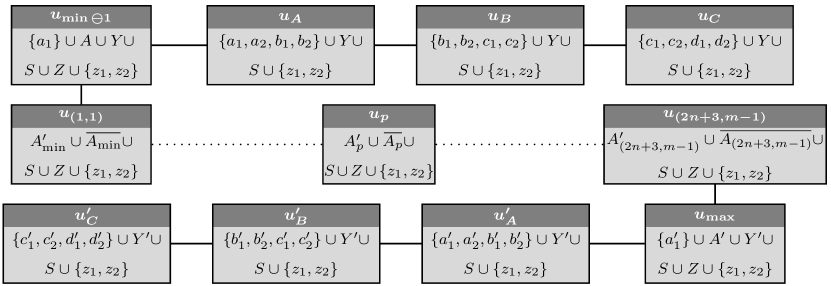
Figure 2. Intended path of the GHD of hypergraph $H$ in the proof of Theorem 3.2

To prove the correctness of our problem reduction, we have to show the two equivalences: first, that $\mathit{ghw}(H)\leq 2$ if and only if $\varphi$ is satisfiable and second, that $\mathit{fhw}(H)\leq 2$ if and only if $\varphi$ is satisfiable. We prove the two directions of these equivalences separately.

Proof of the “if”-direction. First assume that $\varphi$ is satisfiable. It suffices to show that then $H$ has a GHD of width $\leq 2$, because $\mathit{fhw}(H)\leq\mathit{ghw}(H)$ holds. Let $\sigma$ be a satisfying truth assignment. Let us fix for each $j\leq m$, some $k_{j}\in\{1,2,3\}$ such that $\sigma(L^{k_{j}}_{j})=1$. By $l_{j}$, we denote the index of the variable in the literal $L^{k_{j}}_{j}$, that is, $L^{k_{j}}_{j}=x_{l_{j}}$ or $L^{k_{j}}_{j}=\neg x_{l_{j}}$. For $p=(i,j)$, let $k_{p}$ refer to $k_{j}$ and let $L^{k_{p}}_{p}$ refer to $L^{k_{j}}_{j}$. Finally, we define $Z$ as $Z=\{y_{i}\mid\sigma(x_{i})=1\}\cup\{y^{\prime}_{i}\mid\sigma(x_{i})=0\}$.

A GHD $\mathcal{G}=\left<T,(B_{u})_{u\in T},(\lambda_{u})_{u\in T}\right>$ of width 2 for $H$ is constructed as follows. $T$ is a path $u_{C}$, $u_{B}$, $u_{A}$, $u_{\min\ominus 1}$, $u_{\min}$,…, $u_{\max}$, $u^{\prime}_{A}$, $u^{\prime}_{B}$, $u^{\prime}_{C}$. The construction is illustrated in Figure 2. The precise definition of $B_{u}$ and $\lambda_{u}$ is given in Table 1. Clearly, the GHD has width $\leq 2$. We now show that $\mathcal{G}$ is indeed a GHD of $H$:

1. For each edge $e\in E$, there is a node $u\in T$, such that $e\subseteq B_{u}$:

   • $\forall e\in E_{X}:e\subseteq B_{u_{X}}$ for all $X\in\{A,B,C\}$,

   • $\forall e^{\prime}\in E^{\prime}_{X}:e^{\prime}\subseteq B_{u^{\prime}_{X}}$ for all $X\in\{A,B,C\}$,

   • $e_{p}\subseteq B_{u_{p}}$ for $p\in[2n+3;m]^{-}$,

   • $e_{y_{i}}\subseteq B_{u_{\min\ominus 1}}$ (if $y^{\prime}_{i}\in Z$) or $e_{y_{i}}\subseteq B_{u_{\max}}$ (if $y_{i}\in Z$), respectively,

   • $e^{k,0}_{p}\subseteq B_{u_{\min\ominus 1}}$ for $p\in[2n+3;m]^{-}$,

   • $e^{k,1}_{p}\subseteq B_{u_{\max}}$ for $p\in[2n+3;m]^{-}$,

   • $e^{0}_{(0,0)}\subseteq B_{u_{\min\ominus 1}}$, $e^{1}_{(0,0)}\subseteq B_{u_{\max}}$,

   • $e^{0}_{\max}\subseteq B_{u_{\min\ominus 1}}$ and $e^{1}_{\max}\subseteq B_{u_{\max}}$.

   All of the above inclusions can be verified in Table 1.

2. For each vertex $v\in V$, the set $\{u\in T\mid v\in B_{u}\}$ induces a connected subtree of $T$, which is easy to verify in Table 1.

3. For each $u\in T$, $B_{u}\subseteq B(\lambda_{u})$: the only inclusion which cannot be easily verified in Table 1 is $B_{u_{p}}\subseteq B(\lambda_{u_{p}})$. In fact, this is the only place in the proof where we make use of the assumption that $\varphi$ is satisfiable. First, notice that the set $A^{\prime}_{p}\cup\mkern 1.5mu\overline{\mkern-1.5muA_{p}\mkern-1.5mu}\mkern 1.5mu\cup S\cup\{z_{1},z_{2}\}$ is clearly a subset of $B(\lambda_{u_{p}})$. It remains to show that $Z\subseteq B(\lambda_{u_{p}})$ holds for arbitrary $p\in[2n+3;m]^{-}$. We show this property by a case distinction on the form of $L^{k_{p}}_{p}$.

   Case (1): First, assume that $L^{k_{p}}_{p}=x_{l_{j}}$ holds. Then $\sigma(x_{l_{j}})=1$ and, therefore, $y^{\prime}_{l_{j}}\not\in Z$. But, by definition of $e^{k_{p},0}_{p}$ and $e^{k_{p},1}_{p}$, vertex $y^{\prime}_{l_{j}}$ is the only element of $Y\cup Y^{\prime}$ not contained in $B(\lambda_{u_{p}})$. Since $Z\subseteq(Y\cup Y^{\prime})$ and $y^{\prime}_{l_{j}}\not\in Z$, we have that $Z\subseteq B(\lambda_{u_{p}})$.

   Case (2): Now assume that $L^{k_{p}}_{p}=\neg x_{l_{j}}$ holds. Then $\sigma(x_{l_{j}})=0$ and, therefore, $y_{l_{j}}\not\in Z$. But, by definition of $e^{k_{p},0}_{p}$ and $e^{k_{p},1}_{p}$, vertex $y_{l_{j}}$ is the only element of $Y\cup Y^{\prime}$ not contained in $B(\lambda_{u_{p}})$. Since $Z\subseteq(Y\cup Y^{\prime})$ and $y_{l_{j}}\not\in Z$, we have that $Z\subseteq B(\lambda_{u_{p}})$.

Two crucial lemmas. Before we prove the “only if’-direction, we define the notion of complementary edges and state two important lemmas related to this notion.

Definition 3.4.

Let $e$ and $e^{\prime}$ be two edges from the hypergraph $H$ as defined before. We say $e^{\prime}$ is the complementary edge of $e$ (or, simply, $e,e^{\prime}$ are complementary edges) whenever

• $e\cap S=S\setminus S^{\prime}$ for some $S^{\prime}\subseteq S$ and

• $e^{\prime}\cap S=S^{\prime}$.

Observe that for every edge in our construction that covers $S\setminus S^{\prime}$ for some $S^{\prime}\subseteq S$ there is a complementary edge that covers $S^{\prime}$, for example $e^{k,0}_{p}$ and $e^{k,1}_{p}$, $e^{0}_{(0,0)}$ and $e^{1}_{(0,0)}$, and so on. In particular there is no edge that covers $S$ completely. Moreover, consider arbitrary subsets $S_{1},S_{2}$ of $S$, s.t. (syntactically) $S\setminus S_{i}$ is part of the definition of $e_{i}$ for some $e_{i}\in E(H)$ with $i\in\{1,2\}$. Then $S_{1}$ and $S_{2}$ are disjoint.

We now present two lemmas needed for the “only if”-direction.

Lemma 3.5.

Let $\mathcal{F}=\left<T,(B_{u})_{u\in T},(\gamma_{u})_{u\in T}\right>$ be an FHD of width $\leq 2$ of the hypergraph $H$ constructed above. For every node $u$ with $S\cup\{z_{1},z_{2}\}\subseteq B_{u}$ and every pair $e,e^{\prime}$ of complementary edges, it holds that $\gamma_{u}(e)=\gamma_{u}(e^{\prime})$.

Proof.

First, we try to cover $z_{1}$ and $z_{2}$. For $z_{1}$ we have to put total weight $1$ on the edges in $E^{0}$, and to cover $z_{2}$ we have to put total weight $1$ on the edges in $E^{1}$, where

$$E^{0}= \{e^{k,0}_{p}\mid p\in[2n+3;m]^{-}\mbox{ and }1\leq k\leq 3\}\;\cup$$

$$\{e^{0}_{(0,0)},e^{0}_{\max}\}\;\cup$$

$$\{\{a_{1},b_{1}\}\cup M_{1},\{b_{1},c_{1}\}\cup M_{1},\{c_{1},d_{1}\}\cup M_{1}\}\;\cup$$

$$\{\{a^{\prime}_{1},b^{\prime}_{1}\}\cup M^{\prime}_{1},\{b^{\prime}_{1},c^{\prime}_{1}\}\cup M^{\prime}_{1},\{c^{\prime}_{1},d^{\prime}_{1}\}\cup M^{\prime}_{1}\}$$

$$E^{1}= \{e^{k,1}_{p}\mid p\in[2n+3;m]^{-}\mbox{ and }1\leq k\leq 3\}\;\cup$$

$$\{e^{1}_{(0,0)},e^{1}_{\max}\}\;\cup$$

$$\{\{a_{2},b_{2}\}\cup M_{2},\{b_{2},c_{2}\}\cup M_{2},\{c_{2},d_{2}\}\cup M_{2}\}\;\cup$$

$$\{\{a^{\prime}_{2},b^{\prime}_{2}\}\cup M^{\prime}_{2},\{b^{\prime}_{2},c^{\prime}_{2}\}\cup M^{\prime}_{2},\{c^{\prime}_{2},d^{\prime}_{2}\}\cup M^{\prime}_{2}\}$$

In order to also cover $S$ with weight 2, we are only allowed to assign weights to the above edges. Let $S_{i}$ be a subset of $S$, s.t. $S\setminus S_{i}\subseteq e^{0}_{i}$, where $e^{0}_{i}\in E^{0}$. Suppose $\gamma_{u}(e^{0}_{i})=w_{i}$. Still, we need to put weight $1$ on the vertices in $S_{i}$. In order to do so, we can put at most weight $1-w_{i}$ on the edges in $E^{0}\setminus\{e^{0}_{i}\}$, which covers $S_{i}$ with weight at most $1-w_{i}$. The only edge in $E^{1}$ that intersects $S_{i}$ is the complementary edge $e^{1}_{i}$ of $e^{0}_{i}$. Hence, we have to set $\gamma_{u}(e^{1}_{i})\geq w_{i}$. This holds for all edges $e^{1}\in E^{1}$. Moreover, recall that both $\sum_{e^{0}\in E^{0}}\gamma_{u}(e^{0})=1$ and $\sum_{e^{1}\in E^{1}}\gamma_{u}(e^{1})=1$ hold. Hence, we cannot afford to set $\gamma_{u}(e_{i}^{1})>w_{i}$ for some $i$, since this would lead to $\sum_{e^{1}\in E^{1}}\gamma_{u}(e^{1})>1$. We thus have $\gamma_{u}(e_{i}^{0})=\gamma_{u}(e_{i}^{1})=w_{i}$ for every $e_{i}^{0}\in E^{0}$ and its complementary edge $e_{i}^{1}\in E^{1}$. ∎

Lemma 3.6.

Let $\mathcal{F}=\left<T,(B_{u})_{u\in T},(\gamma_{u})_{u\in T}\right>$ be an FHD of width $\leq 2$ of the hypergraph $H$ constructed above and let $p\in[2n+3;m]^{-}$. For every node $u$ with $S\cup A^{\prime}_{p}\cup\mkern 1.5mu\overline{\mkern-1.5muA_{p}\mkern-1.5mu}\mkern 1.5mu\cup\{z_{1},z_{2}\}\subseteq B_{u}$, the only way to cover $S\cup A^{\prime}_{p}\cup\mkern 1.5mu\overline{\mkern-1.5muA_{p}\mkern-1.5mu}\mkern 1.5mu\cup\{z_{1},z_{2}\}$ by a fractional edge cover $\gamma$ of weight $\leq 2$ is by putting non-zero weight exclusively on edges $e^{k,0}_{p}$ and $e^{k,1}_{p}$ with $k\in\{1,2,3\}$. Moreover, $\sum_{k=1}^{3}\gamma(e^{k,0}_{p})=1$ and $\sum_{k=1}^{3}\gamma(e^{k,1}_{p})=1$ must hold.

Proof.

As in the proof of Lemma 3.5, to cover $z_{1}$ we have to put weight $1$ on the edges in $E^{0}$ and to cover $z_{2}$ we have to put weight $1$ on the edges in $E^{1}$, where $E^{0}$ and $E^{1}$ are defined as in the proof of Lemma 3.5. Since we have $0pt(\mathcal{F})\leq 2$, we have to cover $A^{\prime}_{p}\cup\mkern 1.5mu\overline{\mkern-1.5muA_{p}\mkern-1.5mu}\mkern 1.5mu\cup S$ with the weight already put on the edges in $E^{0}\cup E^{1}$. In order to cover $A^{\prime}_{p}$, we have to put weight 1 on the edges in $E^{1}_{p}$, where

$$E^{1}_{p}=\{e^{k,1}_{r}\mid r\geq p\}\cup\{e^{1}_{\max}\}.$$

Notice that, $E^{1}_{p}\subseteq E^{1}$ and therefore $\sum_{e\in E^{1}\setminus E^{1}_{p}}\gamma_{u}(e)=0$. Similar, in order to cover $\mkern 1.5mu\overline{\mkern-1.5muA_{p}\mkern-1.5mu}\mkern 1.5mu$, we have to put weight 1 on the edges in $E^{0}_{p}$, where

$$E^{0}_{p}=\{e^{k,0}_{s}\mid s\leq p\}\cup\{e^{0}_{(0,0)}\}.$$

Again, since $E^{0}_{p}\subseteq E^{0}$, $\sum_{e\in E^{0}\setminus E^{0}_{p}}\gamma_{u}(e)=0$. It remains to cover $S\cup\{z_{1},z_{2}\}$. By Lemma 3.5, in order to cover $S$, $z_{1}$ and $z_{2}$, we have to put the same weight $w$ on complementary edges $e$ and $e^{\prime}$. The only complementary edges in the sets $E^{0}_{p}$ and $E^{1}_{p}$ are edges of the form $e^{k,0}_{p}$ and $e^{k,1}_{p}$ with $k\in\{1,2,3\}$. In total, we thus have $\sum_{k=1}^{3}e^{k,0}_{p}=1$ and $\sum_{k=1}^{3}e^{k,1}_{p}=1$. ∎

Proof of the “only if”-direction. It remains to show that $\varphi$ is satisfiable if $H$ has a GHD or FHD of width $\leq 2$. Due to the inequality $\mathit{fhw}(H)\leq\mathit{ghw}(H)$, it suffices to show that $\varphi$ is satisfiable if $H$ has an FHD of width $\leq 2$. For this, let $\mathcal{F}=\left<T,(B_{u})_{u\in T},(\gamma_{u})_{u\in T}\right>$ be such an FHD. Let $u_{A},u_{B},u_{C}$ and $u^{\prime}_{A},u^{\prime}_{B},u^{\prime}_{C}$ be the nodes that are guaranteed by Lemma 3.1. We state several properties of the path connecting $u_{A}$ and $u^{\prime}_{A}$, which heavily rely on Lemmas 3.5 and 3.6.

Claim A. The nodes $u^{\prime}_{A},u^{\prime}_{B},u^{\prime}_{C}$ (resp. $u_{A},u_{B},u_{C}$) are not on the path from $u_{A}$ to $u_{C}$ (resp. $u^{\prime}_{A}$ to $u^{\prime}_{C}$).

Proof of Claim A. We only show that none of the nodes $u^{\prime}_{i}$ with $i\in\{A,B,C\}$ is on the path from $u_{A}$ to $u_{C}$. The other property is shown analogously. Suppose to the contrary that some $u^{\prime}_{i}$ is on the path from $u_{A}$ to $u_{C}$. Since $u_{B}$ is also on the path between $u_{A}$ and $u_{C}$ we distinguish two cases:

• Case (1): $u^{\prime}_{i}$ is on the path between $u_{A}$ and $u_{B}$; then $\{b_{1},b_{2}\}\subseteq B_{u^{\prime}_{i}}$. This contradicts the property shown in Lemma 3.1 that $u^{\prime}_{i}$ cannot cover any vertices outside $H^{\prime}_{0}$.

• Case (2): $u^{\prime}_{i}$ is on the path between $u_{B}$ and $u_{C}$; then $\{c_{1},c_{2}\}\subseteq B_{u^{\prime}_{i}}$, which again contradicts Lemma 3.1.

Hence, the paths from $u_{A}$ to $u_{C}$ and from $u^{\prime}_{A}$ to $u^{\prime}_{C}$ are indeed disjoint. $\hfill\diamond$

Claim B. The following equality holds: $\mathit{nodes}(A\cup A^{\prime},\mathcal{F})\cap\{u_{A},u_{B},u_{C},u^{\prime}_{A},u^{\prime}_{B},u^{\prime}_{C}\}=\emptyset$.

Proof of Claim B. Suppose to the contrary that there is a $u_{X}$ (the proof for $u^{\prime}_{X}$ is analogous) for some $X\in\{A,B,C\}$, s.t. $u_{X}\in\mathit{nodes}(A\cup A^{\prime},\mathcal{F})$; then there is some $a\in(A\cup A^{\prime})$, s.t. $a\in B_{u_{X}}$. This contradicts the property shown in Lemma 3.1 that $u_{X}$ cannot cover any vertices outside $H_{0}$. $\hfill\diamond$

We are now interested in the sequence of nodes $\hat{u}_{i}$ that cover the edges $e^{0}_{(0,0)},e_{\min},e_{\min\oplus 1}$, …, $e_{\max\ominus 1}$, $e_{\max}$. Before we formulate Claim C, it is convenient to introduce the following notation. To be able to refer to the edges $e^{0}_{(0,0)}$, $e_{\min}$, $e_{\min\oplus 1}$, …, $e_{\max\ominus 1}$, $e^{1}_{\max}$ in a uniform way, we use $e_{\min\ominus 1}$ as synonym of $e^{0}_{(0,0)}$ and $e_{\max}$ as synonym of $e^{1}_{\max}$. We can thus define the natural order $e_{\min\ominus 1}<e_{\min}<e_{\min\oplus 1}<\dots<e_{\max\ominus 1}<e_{\max}$ on these edges.

Claim C. The FHD $\mathcal{F}$ has a path containing nodes $\hat{u}_{1},\dots,$ $\hat{u}_{N}$ for some $N$, such that the edges $e_{\min\ominus 1},e_{\min}$, $e_{\min\oplus 1}$, …, $e_{\max\ominus 1}$, $e_{\max}$ are covered in this order. More formally, there is a mapping $f:\{\min\ominus 1,$ $\ldots,\max\}\rightarrow\{1,\ldots,N\}$, s.t.

• $\hat{u}_{f(p)}$ covers $e_{p}$ and

• if $p<p^{\prime}$ then $f(p)\leq f(p^{\prime})$.

By a path containing nodes $\hat{u}_{1},\dots,\hat{u}_{N}$ we mean that $\hat{u}_{1}$ and $\hat{u}_{N}$ are nodes in $\mathcal{F}$, such that the nodes $\hat{u}_{2},\dots,\hat{u}_{N-1}$ lie (in this order) on the path from $\hat{u}_{1}$ to $\hat{u}_{N}$. Of course, the path from $\hat{u}_{1}$ to $\hat{u}_{N}$ may also contain further nodes, but we are not interested in whether they cover any of the edges $e_{p}$.

Proof of Claim C. Suppose to the contrary that no such path exists. Let $p\geq\min$ be the maximal value such that there is a path containing nodes $\hat{u}_{1},\hat{u}_{2},\ldots,\hat{u}_{l}$, which cover $e_{\min\ominus 1},\ldots,e_{p}$ in this order. Clearly, there exists a node $\hat{u}$ that covers $e_{p\oplus 1}=A^{\prime}_{p\oplus 1}\cup\mkern 1.5mu\overline{\mkern-1.5muA_{p\oplus 1}\mkern-1.5mu}\mkern 1.5mu$. We distinguish four cases:

• Case (1): $\hat{u}_{1}$ is on the path from $\hat{u}$ to all other nodes $\hat{u}_{i}$, with $1<i\leq l$. By the connectedness condition, $\hat{u}_{1}$ covers $A^{\prime}_{p}$. Hence, in total $\hat{u}_{1}$ covers $A^{\prime}_{p}\cup A$ with $A^{\prime}_{p}=\{a^{\prime}_{\min},\dots,a^{\prime}_{p}\}$ and $A=\{a_{\min},\dots,a_{\max}\}$. Then $\hat{u}_{1}$ covers all edges $e_{\min\ominus 1},\ldots,e_{p}$. Therefore, the path containing nodes $\hat{u}_{1}$ and $\hat{u}$ covers $e_{\min\ominus 1},\ldots,$ $e_{p\oplus 1}$ in this order, which contradicts the maximality of $p$.

• Case (2): $\hat{u}=\hat{u}_{1}$, hence, $\hat{u}_{1}$ covers $A^{\prime}_{p\oplus 1}\cup A$ with $A^{\prime}_{p\oplus 1}=\{a^{\prime}_{\min},\dots,a^{\prime}_{p\oplus 1}\}$ and $A=\{a_{\min},\dots$, $a_{\max}\}$. Then, $\hat{u}_{1}$ covers all $e_{\min\ominus 1},\ldots,e_{p\oplus 1}$, which contradicts the maximality of $p$.

• Case (3): $\hat{u}$ is on the path from $\hat{u}_{1}$ to $\hat{u}_{l}$ and $\hat{u}\neq\hat{u}_{1}$. Hence, $\hat{u}$ is between two nodes $\hat{u}_{i}$ and $\hat{u}_{i+1}$ for some $1\leq i<l$ or $\hat{u}=\hat{u}_{i+1}$ for some $1\leq i<l-1$. The following arguments hold for both cases. Now, there is some $q\leq p$, such that $e_{q}$ is covered by $\hat{u}_{i+1}$ and $e_{q\ominus 1}$ is covered by $\hat{u}_{i}$. Therefore, $\hat{u}$ covers $\mkern 1.5mu\overline{\mkern-1.5muA_{q}\mkern-1.5mu}\mkern 1.5mu$ either by the connectedness condition (if $\hat{u}$ is between $\hat{u}_{i}$ and $\hat{u}_{i+1}$) or simply because $\hat{u}=\hat{u}_{i+1}$. Hence, in total, $\hat{u}$ covers $A^{\prime}_{p\oplus 1}\cup\mkern 1.5mu\overline{\mkern-1.5muA_{q}\mkern-1.5mu}\mkern 1.5mu$ with $A^{\prime}_{p\oplus 1}=\{a^{\prime}_{\min},\dots,a^{\prime}_{p\oplus 1}\}$ and $\mkern 1.5mu\overline{\mkern-1.5muA_{q}\mkern-1.5mu}\mkern 1.5mu=\{a_{q},a_{q\oplus 1},\dots,a_{p},a_{p\oplus 1},\dots a_{\max}\}$. Then, $\hat{u}$ covers all edges $e_{q},e_{q\oplus 1},\ldots,e_{p\oplus 1}$. Therefore, the path containing nodes $\hat{u}_{1},\dots,\hat{u}_{i},\hat{u}$ covers $e_{\min\ominus 1},\ldots,e_{p\oplus 1}$ in this order, which contradicts the maximality of $p$.

• Case (4): There is a $u^{*}$ on the path from $\hat{u}_{1}$ to $\hat{u}_{l}$, such that the paths from $\hat{u}_{1}$ to $\hat{u}$ and from $\hat{u}$ to $\hat{u}_{l}$ go through $u^{*}$ and, moreover, $u^{*}\neq\hat{u}_{1}$. Then, $u^{*}$ is either between $\hat{u}_{i}$ and $\hat{u}_{i+1}$ for some $1\leq i<l$ or $u^{*}=\hat{u}_{i+1}$ for some $1\leq i<l-1$. The following arguments hold for both cases. There is some $q\leq p$, such that $e_{q}$ is covered by $\hat{u}_{i+1}$ and $e_{q\ominus 1}$ is covered by $\hat{u}_{i}$. By the connectedness condition, $u^{*}$ covers

  • $A^{\prime}_{p}=\{a^{\prime}_{\min},\ldots,a^{\prime}_{p}\}$, since $u^{*}$ is on the path from $\hat{u}$ to $\hat{u}_{l}$, and

  • $\mkern 1.5mu\overline{\mkern-1.5muA\mkern-1.5mu}\mkern 1.5mu_{q}=\{a_{q},\dots,a_{p},a_{p\oplus 1},\dots a_{\max}\}$, since $u^{*}$ is on the path from $\hat{u}_{1}$ to $\hat{u}_{i+1}$ or $u^{*}=\hat{u}_{i+1}$.

  Then $u^{*}$ covers all edges $e_{q},e_{q\oplus 1},\ldots,e_{p}$. Therefore, the path containing the nodes $\hat{u}_{1},\ldots,\hat{u}_{i}$, $u^{*}$, $\hat{u}$ covers $e_{\min\ominus 1},\ldots,e_{p\oplus 1}$ in this order, which contradicts the maximality of $p$. $\hfill\diamond$

So far we have shown, that there are three disjoint paths from $u_{A}$ to $u_{C}$, from $u^{\prime}_{A}$ to $u^{\prime}_{C}$ and from $\hat{u}_{1}$ to $\hat{u}_{N}$, respectively. It is easy to see, that $u_{A}$ is closer to the path $\hat{u}_{1}$, …, $\hat{u}_{N}$ than $u_{B}$ and $u_{C}$, since otherwise $u_{B}$ and $u_{C}$ would have to cover $a_{1}$ as well, which is impossible by Lemma 3.1. The same also holds for $u^{\prime}_{A}$. In the next claims we will argue that the path from $u_{A}$ to $u^{\prime}_{A}$ goes through some node $\hat{u}$ of the path from $\hat{u}_{1}$ to $\hat{u}_{N}$. We write $\pi(\hat{u}_{1},\hat{u}_{N})$ as a short-hand notation for the path from $\hat{u}_{1}$ to $\hat{u}_{N}$. Next, we state some important properties of $\pi(\hat{u}_{1},\hat{u}_{N})$ and the path from $u_{A}$ to $u_{A}^{\prime}$.

Claim D. In the FHD $\mathcal{F}$ of $H$ of width $\leq 2$, the path from $u_{A}$ to $u^{\prime}_{A}$ has non-empty intersection with $\pi(\hat{u}_{1},\hat{u}_{N})$.

Proof of Claim D. Suppose to the contrary that the path from $u_{A}$ to $u^{\prime}_{A}$ is disjoint from $\pi(\hat{u}_{1},\hat{u}_{N})$. We distinguish three cases:

• Case (1): $u_{A}$ is on the path from $u^{\prime}_{A}$ to (some node in) $\pi(\hat{u}_{1},\hat{u}_{N})$. Then, by the connectedness condition, $u_{A}$ must contain $a^{\prime}_{1}$, which contradicts Lemma 3.1.

• Case (2): $u^{\prime}_{A}$ is on the path from $u_{A}$ to $\pi(\hat{u}_{1},\hat{u}_{N})$. Analogously to Case (1), we get a contradiction by the fact that then $u^{\prime}_{A}$ must contain $a_{1}$.

• Case (3): There is a node $u^{*}$ on the path from $u_{A}$ to $u^{\prime}_{A}$, which is closest to $\pi(\hat{u}_{1},\hat{u}_{N})$, i.e., $u^{*}$ lies on the path from $u_{A}$ to $u^{\prime}_{A}$ and both paths, the one connecting $u_{A}$ with $\pi(\hat{u}_{1},\hat{u}_{N})$ and the one connecting $u^{\prime}_{A}$ with $\pi(\hat{u}_{1},\hat{u}_{N})$, go through $u^{*}$. Hence, by the connectedness condition, the bag of $u^{*}$ contains $S\cup\{z_{1},z_{2},$ $a_{1},a^{\prime}_{1}\}$. By Lemma 3.5, in order to cover $S\cup\{z_{1},z_{2}\}$ with weight $\leq 2$, we are only allowed to put non-zero weight on pairs of complementary edges. However, then it is impossible to achieve also weight $\geq 1$ on $a_{1}$ and $a^{\prime}_{1}$ at the same time. $\hfill\diamond$

(a)

(b)

Figure 3. Arrangement of the nodes $\hat{u}_{1}$, $\hat{u}$, $\hat{u}^{\prime}$, and $\hat{u}_{N}$ from Claim E (a) and Claim G (b).

Claim E. In the FHD $\mathcal{F}$ of $H$ of width $\leq 2$ there are two distinct nodes $\hat{u}$ and $\hat{u}^{\prime}$ in the intersection of the path from $u_{A}$ to $u^{\prime}_{A}$ with $\pi(\hat{u}_{1},\hat{u}_{N})$, s.t. $\hat{u}$ is the node in $\pi(\hat{u}_{1},\hat{u}_{N})$ closest to $u_{A}$ and $\hat{u}^{\prime}$ is the node in $\pi(\hat{u}_{1},\hat{u}_{N})$ closest to $u^{\prime}_{A}$. Then, on the path $\pi(\hat{u}_{1},\hat{u}_{N})$, $\hat{u}$ comes before $\hat{u}^{\prime}$. See Figure 3 (a) for a graphical illustration of the arrangement of the nodes $\hat{u}_{1}$, $\hat{u}$, $\hat{u}^{\prime}$, and $\hat{u}_{N}$ on the path $\pi(\hat{u}_{1},\hat{u}_{N})$.

Proof of Claim E. First, we show that $\hat{u}$ and $\hat{u}^{\prime}$ are indeed distinct. Suppose towards a contradiction that they are not, i.e. $\hat{u}=\hat{u}^{\prime}$. Then, by connectedness, $\hat{u}$ has to cover $S\;\cup$ $\{z_{1},z_{2}\}$, because $S\;\cup$ $\{z_{1},z_{2}\}$ is contained in $B_{u_{A}}$ and in $B_{u^{\prime}_{A}}$. Moreover, again by connectedness, $\hat{u}$ also has to cover $\{a_{1},a^{\prime}_{1}\}$, because $a_{1}$ is contained in $B_{\hat{u}_{1}}$ and in $B_{u_{A}}$ and $a^{\prime}_{1}$ is contained in $B_{\hat{u}_{N}}$ and in $B_{u^{\prime}_{A}}$. As in Case (3) in the proof of Claim D, this is impossible by Lemma 3.5. Hence, $\hat{u}$ and $\hat{u}^{\prime}$ are distinct.

Second, we show that, on the path from $\hat{u}_{1}$ to $\hat{u}_{N}$, the node $\hat{u}$ comes before $\hat{u}^{\prime}$. Suppose to the contrary that $\hat{u}^{\prime}$ comes before $\hat{u}$. Then, by the connectedness condition, $\hat{u}$ covers the following (sets of) vertices:

• $a^{\prime}_{1}$, since we are assuming that $\hat{u}^{\prime}$ comes before $\hat{u}$, i.e., $\hat{u}$ is on the path from $\hat{u}_{N}$ to $u^{\prime}_{A}$;

• $a_{1}$, since $\hat{u}$ is on the path from $\hat{u}_{1}$ to $u_{A}$;

• $S\cup\{z_{1},z_{2}\}$, since $\hat{u}$ is on the path from $u_{A}$ to $u^{\prime}_{A}$.

In total, $\hat{u}$ has to cover all vertices in $S\;\cup$ $\left\{z_{1},z_{2},a_{1},a^{\prime}_{1}\right\}$. Again, by Lemma 3.5, this is impossible with weight $\leq 2$. $\hfill\diamond$

Claim F. In the FHD $\mathcal{F}$ of $H$ of width $\leq 2$ the path $\pi(\hat{u}_{1},\hat{u}_{N})$ has at least 3 nodes $\hat{u}_{i}$, i.e., $N\geq 3$.

Proof of Claim F. First, it is easy to verify that $N\geq 2$ must hold. Otherwise, a single node would have to cover $\{e_{\min\ominus 1},e_{\min}$, $e_{\min\oplus 1}$, …, $e_{\max\ominus 1}$, $e_{\max}\}$ and, hence, in particular, $S\cup\{z_{1},z_{2},a_{1},a^{\prime}_{1}\}$, which is impossible as we have already seen in Case (3) of the proof of Claim D.

It remains to prove $N\geq 3$. Suppose to the contrary that $N=2$. By the problem reduction, hypergraph $H$ has distinct edges $e_{\min\ominus 1}$, $e_{\min}$ and $e_{\max}$. Hence, $\hat{u}_{1}$ covers at least $e_{\min\ominus 1}$ and $\hat{u}_{2}$ covers at least $e_{\max}$. Recall from Claim E the nodes $\hat{u}$ and $\hat{u}^{\prime}$, which constitute the endpoints of the intersection of the path from $u_{A}$ to $u^{\prime}_{A}$ with the path $\pi(\hat{u}_{1},\hat{u}_{N})$, cf. Figure 3(a). Here we are assuming $N=2$. We now show that, by the connectedness condition of FHDs, the nodes $\hat{u}$ and $\hat{u}^{\prime}$ must cover certain vertices, which will lead to a contradiction by Lemma 3.5.

• vertices covered by $\hat{u}$: node $\hat{u}$ is on the path between $u_{A}$ and $u^{\prime}_{A}$. Hence, it covers $S\cup\{z_{1},z_{2}\}$. Moreover, $\hat{u}$ is on the path between $\hat{u}_{1}$ and $u_{A}$ (or even coincides with $\hat{u}_{1}$). Hence, it also covers $a_{1}$. In total, $\hat{u}$ covers at least $S\cup\{z_{1},z_{2},a_{1}\}$.

• vertices covered by $\hat{u}^{\prime}$: node $\hat{u}^{\prime}$ is on the path between $u_{A}$ and $u^{\prime}_{A}$. Hence, it covers $S\cup\{z_{1},z_{2}\}$. Moreover, $\hat{u}^{\prime}$ is on the path between $\hat{u}_{2}$ and $u^{\prime}_{A}$ (or even coincides with $\hat{u}_{2}$). Hence, it also covers $a^{\prime}_{1}$. In total, $\hat{u}^{\prime}$ covers at least $S\cup\{z_{1},z_{2},a^{\prime}_{1}\}$.

One of the nodes $\hat{u}_{1}$ or $\hat{u}_{2}$ must also cover the edge $e_{\min}$. We inspect these 2 cases separately:

• Case (1): suppose that the edge $e_{\min}$ is covered by $\hat{u}_{1}$. Then, $\hat{u}_{1}$ covers vertex $a^{\prime}_{\min}$, which is also covered by $\hat{u}_{2}$. Hence, also $\hat{u}$ covers $a^{\prime}_{\min}$. In total, $\hat{u}$ covers $S\cup\{z_{1},z_{2},a_{1},a^{\prime}_{\min}\}$. However, by Lemma 3.5, we know that, to cover $S\cup\{z_{1},z_{2}\}$ with weight $\leq 2$, we are only allowed to put non-zero weight on pairs of complementary edges. Hence, it is impossible to achieve also weight $\geq 1$ on $a_{1}$ and on $a^{\prime}_{\min}$ at the same time.

• Case (2): suppose that the edge $e_{\min}$ is covered by $\hat{u}_{2}$. Then, $\hat{u}_{2}$ covers vertex $a_{\min}$ (actually, it even covers all of $A$), which is also covered by $\hat{u}_{1}$. Hence, also $\hat{u}^{\prime}$ covers $a_{\min}$. In total, $\hat{u}^{\prime}$ covers $S\cup\{z_{1},z_{2},a^{\prime}_{1},a_{\min}\}$. Again, this is impossible by Lemma 3.5.

Hence, the path $\pi(\hat{u}_{1},\hat{u}_{N})$ indeed has at least 3 nodes $\hat{u}_{i}$. $\hfill\diamond$

Claim G. In the FHD $\mathcal{F}$ of $H$ of width $\leq 2$ all the nodes $\hat{u}_{2},\ldots,\hat{u}_{N-1}$ are on the path from $u_{A}$ to $u^{\prime}_{A}$. For the nodes $\hat{u}$ and $\hat{u}^{\prime}$ from Claim E, this means that the nodes $\hat{u}_{1},\hat{u},$ $\hat{u}_{2},\hat{u}_{N-1}$, $\hat{u}^{\prime}$, $\hat{u}_{N}$ are arranged in precisely this order on the path $\pi(\hat{u}_{1},\hat{u}_{N})$ from $\hat{u}_{1}$ to $\hat{u}_{N}$, cf. Figure 3 (b). The node $\hat{u}$ may possibly coincide with $\hat{u}_{1}$ and $\hat{u}^{\prime}$ may possibly coincide with $\hat{u}_{N}$.

Proof of Claim G. We have to prove that $\hat{u}$ lies between $\hat{u}_{1}$ and $\hat{u}_{2}$ (not including $\hat{u}_{2}$) and $\hat{u}^{\prime}$ lies between $\hat{u}_{N-1}$ and $\hat{u}_{N}$ (not including $\hat{u}_{N-1}$). For the first property, suppose to the contrary that $\hat{u}$ does not lie between $\hat{u}_{1}$ and $\hat{u}_{2}$ or $\hat{u}=\hat{u}_{2}$. This means, that there exists $i\in\{2,\dots,N-1\}$ such that $\hat{u}$ lies between $\hat{u}_{i}$ and $\hat{u}_{i+1}$, including the case that $\hat{u}$ coincides with $\hat{u}_{i}$. Note that, by Claim E, $\hat{u}$ cannot coincide with $\hat{u}_{N}$, since there is yet another node $\hat{u}^{\prime}$ between $\hat{u}$ and $\hat{u}_{N}$.

By definition of $\hat{u}_{i}$ and $\hat{u}_{i+1}$, there is a $p\in[2n+3;m]$, such that both $\hat{u}_{i}$ and $\hat{u}_{i+1}$ cover $a^{\prime}_{p}$. Then, by the connectedness condition, $\hat{u}$ covers the following (sets of) vertices:

• $a^{\prime}_{p}$, since $\hat{u}$ is on the path from $\hat{u}_{i}$ to $\hat{u}_{i+1}$ (or $\hat{u}$ coincides with $\hat{u}_{i}$),

• $a_{1}$, since $\hat{u}$ is on the path from $\hat{u}_{1}$ to $u_{A}$,

• $S\cup\{z_{1},z_{2}\}$, since $\hat{u}$ is on the path from $u_{A}$ to $u^{\prime}_{A}$.

However, by Lemma 3.5, we know that, to cover $S\cup\{z_{1},z_{2}\}$ with weight $\leq 2$, we are only allowed to put non-zero weight on pairs of complementary edges. Hence, it is impossible to achieve also weight $\geq 1$ on $a^{\prime}_{p}$ and $a_{1}$ at the same time.

It remains to show that $\hat{u}^{\prime}$ lies between $\hat{u}_{N-1}$ and $\hat{u}_{N}$ (not including $\hat{u}_{N-1}$). Suppose to the contrary that it does not. Then, analogously to the above considerations for $\hat{u}$, it can be shown that there exists some $p\in[2n+3;m]$, such that $\hat{u}^{\prime}$ covers the vertices $S\cup\{z_{1},z_{2},a_{p},a^{\prime}_{1}\}$. Again, this is impossible by Lemma 3.5. $\hfill\diamond$

By Claim C, the decomposition $\mathcal{F}$ contains a path $\hat{u}_{1}\cdots\hat{u}_{N}$ that covers the edges $e_{\min\ominus 1},e_{\min}$, $e_{\min\oplus 1}$, …, $e_{\max\ominus 1}$, $e_{\max}$ in this order. We next strengthen this property by showing that every node $\hat{u}_{i}$ covers exactly one edge $e_{p}$.

Claim H. Each of the nodes $\hat{u}_{1},\dots,\hat{u}_{N}$ covers exactly one of the edges $e_{\min\ominus 1}$, $e_{\min}$, $e_{\min\oplus 1}$, …, $e_{\max\ominus 1}$, $e_{\max}$.

Proof of Claim H. We prove this property for the “outer nodes” $\hat{u}_{1}$, $\hat{u}_{N}$ and for the “inner nodes” $\hat{u}_{2}\cdots\hat{u}_{N-1}$ separately. We start with the “outer nodes”. The proof for $\hat{u}_{1}$ and $\hat{u}_{N}$ is symmetric. We thus only work out the details for $\hat{u}_{1}$. Suppose to the contrary that $\hat{u}_{1}$ not only covers $e_{\min\ominus 1}$ but also $e_{\min}$. We distinguish two cases according to the position of node $\hat{u}$ in Figure 3 (b):

• Case (1): $\hat{u}=\hat{u}_{1}$. Then, $\hat{u}_{1}$ has to cover the following (sets of) vertices:

  • $S\cup\{z_{1},z_{2}\}$, since $\hat{u}$ is on the path from $u_{A}$ to $u^{\prime}_{A}$ and we are assuming $\hat{u}=\hat{u}_{1}$.

  • $a_{1}$, since $\hat{u}_{1}$ covers $e_{\min\ominus 1}$,

  • $a^{\prime}_{\min}$, since we are assuming that $\hat{u}_{1}$ also covers $e_{\min}$.

  By applying Lemma 3.5, we may conclude that the set $S\cup\{z_{1},z_{2},a_{1},a^{\prime}_{\min}\}$ cannot be covered by a fractional edge cover of weight $\leq 2$.

• Case (2): $\hat{u}\neq\hat{u}_{1}$. Then $\hat{u}$ is on the path from $\hat{u}_{1}$ to $\hat{u}_{2}$. Hence, $\hat{u}$ has to cover the following (sets of) vertices:

  • $S\cup\{z_{1},z_{2}\}$, since $\hat{u}$ is on the path from $u_{A}$ to $u^{\prime}_{A}$,

  • $a_{1}$, since $\hat{u}$ is on the path from $u_{A}$ to $\hat{u}_{1}$,

  • $a^{\prime}_{\min}$, since $\hat{u}$ is on the path from $\hat{u}_{1}$ to $\hat{u}_{2}$.

  As in Case (1) above, $S\cup\{z_{1},z_{2},a_{1},a^{\prime}_{\min}\}$ cannot be covered by a fractional edge cover of weight $\leq 2$ due to Lemma 3.5.

It remains to consider the “inner” nodes $\hat{u}_{i}$ with $2\leq i\leq N-1$. Each such $\hat{u}_{i}$ has to cover $S\cup\{z_{1},z_{2}\}$ since all these nodes are on the path from $u_{A}$ to $u^{\prime}_{A}$ by Claim G. Now suppose that $\hat{u}_{i}$ covers $e_{p}=A^{\prime}_{p}\cup\mkern 1.5mu\overline{\mkern-1.5muA_{p}\mkern-1.5mu}\mkern 1.5mu$ for some $p\in\{e_{\min},\dots,e_{\max\ominus 1}\}$. By Lemma 3.6, covering all of the vertices $A^{\prime}_{p}\cup\mkern 1.5mu\overline{\mkern-1.5muA_{p}\mkern-1.5mu}\mkern 1.5mu\cup S\cup\{z_{1},z_{2}\}$ by a fractional edge cover of weight $\leq 2$ requires that we put total weight $1$ on the edges $e^{k,0}_{p}$ and total weight $1$ on the edges $e^{k,1}_{p}$ with $k\in\{1,2,3\}$. However, then it is impossible to cover also $e_{p^{\prime}}$ for some $p^{\prime}$ with $p^{\prime}\neq p$. This concludes the proof of Claim F.$\hfill\diamond$

We can now associate with each $\hat{u}_{i}$ for $1\leq i\leq N$ the corresponding edge $e_{p}$ and write $u_{p}$ to denote the node that covers the edge $e_{p}$. By Claim G, we know that all of the nodes $u_{\min}\dots,u_{\max\ominus 1}$ are on the path from $u_{A}$ to $u^{\prime}_{A}$. Hence, by the connectedness condition, all these nodes cover $S\cup\{z_{1},z_{2}\}$.

We are now ready to construct a satisfying truth assignment $\sigma$ of $\varphi$. For each $i\leq 2n+3$, let $X_{i}$ be the set $B_{u_{(i,1)}}\cap(Y\cup Y^{\prime})$. As $Y\subseteq B_{u_{A}}$ and $Y^{\prime}\subseteq B_{u^{\prime}_{A}}$, the sequence $X_{1}\cap Y,\ldots,X_{2n+3}\cap Y$ is non-increasing and the sequence $X_{1}\cap Y^{\prime},\ldots,X_{2n+3}\cap Y^{\prime}$ is non-decreasing. Furthermore, as all edges $e_{y_{i}}=\{y_{i},y^{\prime}_{i}\}$ must be covered by some node in $\mathcal{F}$, we conclude that for each $i$ and $j$, $y_{j}\in X_{i}$ or $y^{\prime}_{j}\in X_{i}$. Then, there is some $s\leq 2n+2$ such that $X_{s}=X_{s+1}$. Furthermore, all nodes between $u_{(s,1)}$ and $u_{(s+1,1)}$ cover $X_{s}$. We derive a truth assignment for $x_{1},\ldots,x_{n}$ from $X_{s}$ as follows. For each $l\leq n$, we set $\sigma(x_{l})=1$ if $y_{l}\in X_{s}$ and otherwise $\sigma(x_{l})=0$. Note that in the latter case $y^{\prime}_{l}\in X_{s}$.

Claim I. The constructed truth assignment $\sigma$ is a model of $\varphi$.

Proof of Claim I. We have to show that every clause $c_{j}=L_{j}^{1}\vee L_{j}^{2}\vee L_{j}^{3}$ of $\varphi$ is true in $\sigma$. Choose an arbitrary $j\in\{1,\dots,m\}$. We have to show that there exists a literal in $c_{j}$ which is true in $\sigma$. To this end, we inspect the node $u_{(s,j)}$, which, by construction, lies between $u_{(s,1)}$ and $u_{(s+1,1)}$. Let $p=(s,j)$. Then we have $A^{\prime}_{p}\cup\mkern 1.5mu\overline{\mkern-1.5muA_{p}\mkern-1.5mu}\mkern 1.5mu\cup S\cup\{z_{1},z_{2}\}\subseteq B_{u_{p}}$. Moreover, by the definition of $X_{s}$, we also have $X_{s}\subseteq B_{u_{p}}$. By Lemma 3.6, the only way to cover $B_{u_{p}}$ with weight $\leq 2$ is by using exclusively the edges $e^{k,0}_{p}$ and $e^{k,1}_{p}$ with $k\in\{1,2,3\}$. More specifically, we have $\sum_{k=1}^{3}\gamma_{u_{p}}(e^{k,0}_{p})=1$ and $\sum_{k=1}^{3}\gamma_{u_{p}}(e^{k,1}_{p})=1$. Therefore, $\gamma_{u_{p}}(e^{k,0}_{p})>0$ for some $k$. We distinguish two cases depending on the form of literal $L^{k}_{j}$:

• Case (1): First, suppose $L^{k}_{j}=x_{l}$. By Lemma 3.5, complementary edges must have equal weight. Hence, from $\gamma_{u_{p}}(e^{k,0}_{p})>0$ it follows that also $\gamma_{u_{p}}(e^{k,1}_{p})>0$ holds. Thus, the weight on $y^{\prime}_{l}$ is less than $1$, which means that $y^{\prime}_{l}\not\in B(\gamma_{u_{p}})$ and consequently $y^{\prime}_{l}\not\in X_{s}$. Since this implies that $y_{l}\in X_{s}$, we indeed have that $\sigma(x_{l})=1$.

• Case (2): Conversely, suppose $L^{k}_{j}=\neg x_{l}$. Since $\gamma_{u_{p}}(e^{k,0}_{p})>0$, the weight on $y_{l}$ is less than $1$, which means that $y_{l}\not\in B(\gamma_{u_{p}})$ and consequently $y_{l}\not\in X_{s}$. Hence, we have $\sigma(x_{l})=0$.

In either case, literal $L^{k}_{p}$ is satisfied by $\sigma$ and therefore, the $j$-th clause $c_{j}$ is satisfied by $\sigma$. Since $j$ was arbitrarily chosen, $\sigma$ indeed satisfies $\varphi$.$\hfill\diamond$

Claim I completes the proof of Theorem 3.2. ∎

We conclude this section by mentioning that the above reduction is easily extended to $k+\ell$ for arbitrary $\ell\geq 1$: for integer values $\ell$, simply add a clique of $2\ell$ fresh vertices $v_{1},\dots,v_{2\ell}$ to $H$ and connect each $v_{i}$ with each “old” vertex in $H$. Now assume a rational value $\ell\geq 1$, i.e., $\ell=r/q$ for natural numbers $r,q$ with $r>q>0$. To achieve a rational bound $k+r/q$, we add $r$ fresh vertices and add hyperedges $\{v_{i},v_{i\oplus 1},\dots,v_{i\oplus(q-1)}\}$ with $i\in\{1,\dots,r\}$ to $H$, where $a\oplus b$ denotes $a+b$ modulo $r$. Again, we connect each $v_{i}$ with each “old” vertex in $H$. With this construction we can give NP-hardness proofs for any (fractional) $k\geq 3$. For all fractional values $k<3$ (except for $k=2$) different gadgets and ideas might be needed to prove NP-hardness of Check(FHD,$k$), which we leave for future work.

4. Efficient Computation of GHDs

As discussed in Section 1 we are interested in finding a realistic and non-trivial criterion on hypergraphs that makes the Check(GHD, $k$) problem tractable for fixed $k$. We thus propose here such a simple property, namely the bounded intersection of two or more edges.

Definition 4.1.

The intersection width $\mbox{\it iwidth}(H)$ of a hypergraph $H$ is the maximum cardinality of any intersection $e_{1}\cap e_{2}$ of two distinct edges $e_{1}$ and $e_{2}$ of $H$. We say that a hypergraph $H$ has the $i$-bounded intersection property ($i$-BIP) if $\mbox{\it iwidth}(H)\leq i$ holds.

Let $\mathscr{C}$ be a class of hypergraphs. We say that $\mathscr{C}$ has the bounded intersection property (BIP) if there exists some integer constant $i$ such that every hypergraph $H$ in $\mathscr{C}$ has the $i$-BIP. Class $\mathscr{C}$ has the logarithmically-bounded intersection property (LogBIP) if for each of its elements $H$, $\mbox{\it iwidth}(H)$ is ${\mathcal{O}}(\log n)$, where $n$ denotes the size of the hypergraph $H$.

The BIP criterion is indeed non-trivial, as several well-known classes of unbounded $\mathit{ghw}$ enjoy the 1-BIP, such as cliques and grids. Moreover, our empirical study (Fischl et al., 2019) suggests that the overwhelming number of CQs enjoys the $2$-BIP (i.e., one hardly joins two relations over more than 2 attributes). To allow for a yet bigger class of hypergraphs, the BIP can be relaxed as follows.

Definition 4.2.

The $c$-multi-intersection width $c$-miwidth($H$) of a hypergraph $H$ is the maximum cardinality of any intersection $e_{1}\cap\cdots\cap e_{c}$ of $c$ distinct edges $e_{1},\ldots,e_{c}$ of $H$. We say that a hypergraph $H$ has the $i$-bounded $c$-multi-intersection property ($ic$-BMIP) if $\mbox{\it$c$-miwidth($H$)}\leq i$ holds.

Let $\mathscr{C}$ be a class of hypergraphs. We say that $\mathscr{C}$ has the bounded multi-intersection property (BMIP) if there exist constants $c$ and $i$ such that every hypergraph $H$ in $\mathscr{C}$ has the $ic$-BMIP. Class $\mathscr{C}$ of hypergraphs has the logarithmically-bounded multi-intersection property (LogBMIP) if there is a constant $c$ such that for the hypergraphs $H\in\mathscr{C}$, $c$-miwidth($H$) is ${\mathcal{O}}(\log n)$, where $n$ denotes the size of the hypergraph $H$.

Figure 4. Hypergraph $H_{0}$ from Example 4.3

Example 4.3.

Figure 4 shows the hypergraph $H_{0}=(V_{0},E_{0})$ with $ghw(H_{0})=2$ but $hw(H_{0})$=3. (which is from (Gottlob et al., 2009), which, in turn, was inspired by work of Adler (Adler, 2004)). Figure 5 shows an HD of width 3 and Figure 6 shows GHDs of width 2 for the hypergraph $H_{0}$. The BIP and the 3-BMIP of $H_{0}$ is 1. Starting from c=4, the c-BMIP is 0. $\Diamond$

Figure 5. HD of hypergraph $H_{0}$ in Figure 4

The LogBMIP is the most liberal restriction on classes of hypergraphs introduced in Definitions 4.1 and 4.2. The main result in this section will be that the Check(GHD, $k$) problem with fixed $k$ is tractable for any class of hypergraphs satisfying this criterion.

Towards this result, first recall that the difference between HDs and GHDs lies in the “special condition” required by HDs. Assume a hypergraph $H=(V(H),E(H))$ and an arbitrary GHD $\mathcal{H}=\left<T,(B_{u})_{u\in T},(\lambda_{u})_{u\in T}\right>$ of $H$. Then $\mathcal{H}$ is not necessarily an HD, since it may contain a special condition violation (SCV), i.e.: there can exist a node $u$, an edge $e\in\lambda_{u}$ and a vertex $v\in V$, s.t. $v\in e$ (and, hence, $v\in B(\lambda_{u})$), $v\not\in B_{u}$ and $v\in V(T_{u})$. Clearly, if we could be sure that $E(H)$ also contains the edge $e^{\prime}=e\cap B_{u}$, then we would simply replace $e$ in $\lambda_{u}$ by $e^{\prime}$ and would thus get rid of this SCV.

Example 4.4 (Example 4.3 continued).

The GHDs in Figure 6 (a) and (b) violate the special condition in node $u$ since the edge $e_{2}$ containing vertex $v_{2}$ is in $\lambda_{u}$ and $v_{2}$ is in $V(T_{u})$ but not in $B_{u}$. Adding

$$e^{\prime}_{2}=e_{2}\cap B_{u}=\{v_{2},v_{3},v_{9}\}\cap\{v_{3},v_{6},v_{7},v_{9},v_{10}\}=\{v_{3},v_{9}\}$$

to $H_{0}$ and replacing $e_{2}$ with $e^{\prime}_{2}$ in $\lambda_{u}$ would repair the SCV at node $u$ of the GHDs in Figure 6. $\Diamond$

Now our goal is to define a polynomial-time computable function $f$ which, to each hypergraph $H$ and integer $k$, associates a set $f(H,k)$ of additional hyperedges such that $\mathit{ghw}(H)=k$ iff $\mathit{hw}(H^{\prime})=k$ with $H=(V(H),E(H))$ and $H^{\prime}=(V(H),E(H)\cup f(H,k))$. From this it follows immediately that $\mathit{ghw}(H)$ is computable in polynomial time. The function $f$ is defined in such a way that $f(H,k)$ only contains subsets of hyperedges of $H$. Thus, $f$ is a subedge function as described in (Gottlob et al., 2009) and a GHD of the same width can be easily obtained from any HD of $H^{\prime}$. It is easy to see and well-known (Gottlob et al., 2009) that for each subedge function $f$, and each $H$ and $k$, $\mathit{ghw}(H)\leq\mathit{hw}(H\cup f(H,k))\leq\mathit{hw}(H)$. Moreover, for the “limit” subedge function $f^{+}$ where $f^{+}(H,k)$ consists of all possible non-empty subsets of edges of $H$, we have that $\mathit{hw}(H\cup f^{+}(H,k))=\mathit{ghw}(H)$ (Adler, 2004; Gottlob et al., 2009). Of course, in general, $f^{+}$ contains an exponential number of edges. The important point is that our function $f$ will achieve the same, while generating a polynomial and Ptime-computable set of edges only.

(a)

(b)

Figure 6. (a) non bag-maximal vs. (b) bag-maximal GHD of hypergraph $H_{0}$ in Figure 4

We start by introducing a useful property of GHDs, which we will call bag-maximality. Let $\mathcal{H}=\left<T,(B_{u})_{u\in T},(\lambda_{u})_{u\in T}\right>$ be a GHD of some hypergraph $H=(V(H),E(H))$. For each node $u$ in $T$, we have $B_{u}\subseteq B(\lambda_{u})$ by definition of GHDs and, in general, $B(\lambda_{u})\setminus B_{u}$ may be non-empty. We observe that it is sometimes possible to take some vertices from $B(\lambda_{u})\setminus B_{u}$ and add them to $B_{u}$ without violating the connectedness condition. Of course, such an addition of vertices to $B_{u}$ does not violate any of the other conditions of GHDs. Moreover, it does not increase the width.

Definition 4.5.

Let $\mathcal{H}=\left<T,(B_{u})_{u\in T},(\lambda_{u})_{u\in T}\right>$ be a GHD of some hypergraph $H=(V(H),E(H))$. We call $\mathcal{H}$ bag-maximal, if for every node $u$ in $T$, adding a vertex $v\in B(\lambda_{u})\setminus B_{u}$ to $B_{u}$ would violate the connectedness condition.

It is easy to verify that if $H$ has a GHD of width $\leq k$, then it also has a bag-maximal GHD of width $\leq k$.

Lemma 4.6.

For every GHD $\mathcal{H}=\left<T,(B_{u})_{u\in T},(\lambda_{u})_{u\in T}\right>$ of some hypergraph $H=(V(H),E(H))$, there exists a bag-maximal GHD $\mathcal{H}^{\prime}=\left<T,(B^{\prime}_{u})_{u\in T},(\lambda_{u})_{u\in T}\right>$ of $H$, such that $\mathcal{H}$ and $\mathcal{H}^{\prime}$ have the same width.

Proof.

Start with a GHD of width $k$ of $H$. As long as there exists a node $u\in T$ and a vertex $v\in B(\lambda_{u})\setminus B_{u}$, such that $v$ can be added to $B_{u}$ without destroying the GHD properties, select such a node $u$ and vertex $v$ arbitrarily and add $v$ to $B_{u}$. By exhaustive application of this transformation, a bag-maximal GHD of width $k$ of $H$ is obtained. ∎

Example 4.7 (Example 4.4 continued).

Clearly, the GHD in Figure 6(a) violates bag-maximality in node $u^{\prime}$, since the vertices $v_{4}$ and $v_{5}$ can be added to $B_{u^{\prime}}$ without violating any GHD properties. If we add $v_{4}$ and $v_{5}$ to $B_{u^{\prime}}$, then bag $B_{u^{\prime}}$ at node $u^{\prime}$ and the bag at its child node are the same, which allows us to delete one of the nodes. This results in the GHD given in Figure 6(b), which is bag-maximal. In particular, the vertex $v_{2}$ cannot be added to $B_{u_{0}}$: indeed, adding $v_{2}$ to $B_{u_{0}}$ would violate the connectedness condition, since $v_{2}$ is not in $B_{u_{1}}$ but in $B_{u_{2}}$. $\Diamond$

So from now on, we will restrict ourselves w.l.o.g. to bag-maximal GHDs. Before we prove a crucial lemma, we introduce some useful notation:

Definition 4.8.

Let $\mathcal{H}=\left<T,(B_{u})_{u\in T},(\lambda_{u})_{u\in T}\right>$ be an GHD of a hypergraph $H$. Moreover, let $u$ be a node in $\mathcal{H}$ and let $e\in\lambda_{u}$ such that $e\setminus B_{u}\neq\emptyset$ holds. Let $u^{*}$ denote the node closest to $u$, such that $u^{*}$ covers $e$, i.e., $e\subseteq B_{u*}$. Then, we call the path $\pi=(u_{0},u_{1},\ldots,u_{l})$ with $u_{0}=u$ and $u_{l}=u^{*}$ the critical path of $(u,e)$ denoted as $\mathit{critp}(u,e)$.

Lemma 4.9.

Let $\mathcal{H}=\left<T,(B_{u})_{u\in T},(\lambda_{u})_{u\in T}\right>$ be a bag-maximal GHD of a hypergraph $H=(V(H),$ $E(H))$, let $u\in T$, $e\in\lambda_{u}$, and $e\setminus B_{u}\neq\emptyset$. Let $\pi=(u_{0},u_{1},\dots,u_{\ell})$ with $u_{0}=u$ be the critical path of $(u,e)$. Then the following equality holds.

$$e\cap B_{u}=\ \ \ \ e\,\cap\bigcap_{i=1}^{\ell}B(\lambda_{u_{i}})$$

Proof.

“$\subseteq$”: Given that $e\subseteq B_{u_{\ell}}$ and by the connectedness condition, $e\cap B_{u}$ must be a subset of $B_{u_{i}}$ for every $i\in\{1,\dots,\ell\}$. Therefore, $e\cap B_{u}\subseteq e\cap\bigcap_{i=1}^{\ell}B(\lambda_{u_{i}})$ holds.

“$\supseteq$”: Assume to the contrary that there exists some vertex $v\in e$ with $v\not\in B_{u}$ but $v\in\bigcap_{i=1}^{\ell}B(\lambda_{u_{i}})$. By $e\subseteq B_{u_{\ell}}$, we have $v\in B_{u_{\ell}}$. By the connectedness condition, along the path $u_{0},\dots,u_{\ell}$ with $u_{0}=u$, there exists $\alpha\in\{0,\dots,\ell-1\}$, s.t. $v\not\in B_{u_{\alpha}}$ and $v\in B_{u_{\alpha+1}}$. However, by the assumption, $v\in\bigcap_{i=1}^{\ell}B(\lambda_{u_{i}})$ holds. In particular, $v\in B(\lambda_{u_{\alpha}})$. Hence, we could safely add $v$ to $B_{u_{\alpha}}$ without violating the connectedness condition nor any other GHD condition. This contradicts the bag-maximality of $\mathcal{H}$. ∎

Example 4.10 (Example 4.4 continued).

Consider root node $u$ of the GHD in Figure 6(b). We have $e_{2}\in\lambda_{u}$ and $e_{2}\setminus B_{u}=\{v_{2}\}\neq\emptyset$. On the other hand, $e_{2}$ is covered by $u_{2}$. Hence, the critical path of $(u,e_{2})$ is $\pi=(u,u_{1},u_{2})$. It is easy to verify that $e_{2}\cap B_{u}=e_{2}\cap(e_{3}\cup e_{7})\cap(e_{8}\cup e_{2})=\{v_{3},v_{9}\}$ indeed holds. $\Diamond$

We are now ready to prove the main result of this section.

Theorem 4.11.

For every hypergraph class $\mathscr{C}$ that enjoys the LogBMIP, and for every constant $k\geq 1$, the Check(GHD, $k$) problem is tractable, i.e., given a hypergraph $H$, it is feasible in polynomial time to check $\mathit{ghw}(H)\leq k$ and, if so, to compute a GHD of width $k$ of $H$.

Proof.

Let $H=(V(H),E(H))$ be an arbitrary hypergraph. Our goal is to show that there exists a polynomially bounded, polynomial-time computable set $f(H,k)$ of subedges of $H$, such that $\mathit{ghw}(H)=k$ iff $\mathit{hw}(H^{\prime})=k$ with $H^{\prime}=(V(H),E(H)\cup f(H,k))$. By our considerations above, in order to guarantee the equivalence $\mathit{ghw}(H)=k$ iff $\mathit{hw}(H^{\prime})=k$, it suffices to construct $f(H,k)$ in such a way that, in every GHD $\mathcal{G}$ of $H$, for every node $u$ in $\mathcal{G}$, and every edge $e\in\lambda_{u}$, the set $f(H,k)$ contains the subedge $e^{\prime}=e\cap B_{u}$.

Let $\mathcal{H}=\left<T,(B_{u})_{u\in T},(\lambda_{u})_{u\in T}\right>$ be a bag-maximal GHD of $H$, let $u\in T$, $e\in\lambda_{u}$, and $e\setminus B_{u}\neq\emptyset$. Let $\pi=(u_{0},u_{1},\dots,u_{\ell})$ with $u_{0}=u$ be the critical path of $(u,e)$. By Lemma 4.9, the equality $e\cap B_{u}=e\,\cap\bigcap_{i=1}^{\ell}B(\lambda_{u_{i}})$ holds. For $i\in\{1,\dots,\ell\}$, let $\lambda_{u_{i}}=\{e_{i1},\dots,e_{ij_{i}}\}$ with $j_{i}\leq k$. Then $e\,\cap\bigcap_{i=1}^{\ell}B(\lambda_{u_{i}})$ and, therefore, also $e\cap B_{u}$, is of the form

$$e\cap(e_{11}\cup\dots\cup e_{1j_{1}})\cap\dots\cap(e_{\ell 1}\cup\dots\cup e_{\ell j_{\ell}}).$$

We want to construct $f(H,k)$ in such a way that it contains all possible sets $e\cap B_{u}$ of vertices. To this end, we proceed by a stepwise transformation of the above intersection of unions into a union of intersections via distributivity of $\cup$ and $\cap$.

For $i\in\{0,\dots,\ell\}$, let $I_{i}=e\cap\bigcap_{\alpha=1}^{i}B(\lambda_{u_{\alpha}})=e\cap\bigcap_{\alpha=1}^{i}(e_{\alpha 1}\cup\dots\cup e_{\alpha j_{\alpha}})$. Then $I_{0}=e$. For $I_{1}$ we have to distinguish two cases: if $e\in\lambda_{u_{1}}$, then $e\subseteq B(\lambda_{i_{1}})$ and, therefore, $I_{1}=I_{0}$. If $e\not\in\lambda_{u_{1}}$, then $I_{1}=(e\cap e_{11})\cup\dots\cup(e\cap e_{1j_{1}})$. In the latter case, for computing $I_{2}$, we have to go through all sets $(e\cap e_{1\beta})$ with $\beta\in\{1,\dots,j_{1}\}$ and distinguish the two cases if $\{e,e_{1\beta}\}\cap\lambda_{u_{2}}\neq\emptyset$ holds or not. If it holds, then we let $(e\cap e_{1\beta})$ in the disjunction of $I_{1}$ unchanged. Otherwise we replace it by $(e\cap e_{1\beta}\cap e_{21})\cup\dots\cup(e\cap e_{1\beta}\cap e_{2j_{2}})$. This splitting of intersections into unions of intersections can be iterated over all $i\in\{1,\dots,\ell\}$ in order to arrive at $I_{\ell}=e\,\cap\bigcap_{i=1}^{\ell}B(\lambda_{u_{i}})=e\cap B_{u}$, where $I_{\ell}$ is represented as a union of intersections.

We formalize the computation of the intersections in $I_{0}$, …, $I_{\ell}$ by constructing the “$\bigcup\bigcap$-tree” in Algorithm 1 “Union-of-Intersections-Tree”. In a loop over all $i\in\{1,\dots,\ell\}$, we thus compute trees ${\mathcal{T}}_{i}$ such that each node $p$ in ${\mathcal{T}}_{i}$ is labelled by a set $\mathit{label}(p)$ of edges. By $\mathit{int}(p)$ we denote the intersection of the edges in $\mathit{label}(p)$. The parent-child relationship between a node $p$ and its child nodes $p_{1},\dots,p_{j_{\alpha}}$ corresponds to a splitting step, where the intersection $\mathit{int}(p)$ is replaced by the union $(\mathit{int}(p)\cap e_{\alpha 1})\cup\dots\cup(\mathit{int}(p)\cap e_{\alpha j_{\alpha}})$. It can be proved by a straightforward induction on $i$ that, in the tree ${\mathcal{T}}_{i}$, the union of $\mathit{int}(p)$ over all leaf nodes $p$ of ${\mathcal{T}}_{i}$ yields precisely the union-of-intersections representation of $I_{i}$.

We observe that, in the tree ${\mathcal{T}}_{\ell}$, each node has at most $k$ child nodes. Nevertheless, ${\mathcal{T}}_{\ell}$ can become exponentially big since we have no appropriate bound on the length $\ell$ of the critical path. Recall, however, that we are assuming the LogBMIP, i.e., there exists a constant $c>1$, s.t. any intersection of $\geq c$ edges of $H$ has at most $a\log n$ elements, where $a$ is a constant and $n$ denotes the size of $H$. Now let ${\mathcal{T}}^{*}$ be the reduced $\bigcup\bigcap$-tree, which is obtained from ${\mathcal{T}}_{\ell}$ by cutting off all nodes of depth greater than $c-1$. Clearly, ${\mathcal{T}}^{*}$ has at most $k^{c-1}$ leaf nodes and the total number of nodes in ${\mathcal{T}}^{*}$ is bounded by $(c-1)k^{c-1}$.

The set $f(H,k)$ of subedges that we add to $H$ will consist in all possible sets $I_{\ell}$ that we can obtain from all possible critical paths $\pi=(u_{0},u_{1},\dots,u_{\ell})$ in all possible bag-maximal GHDs $\mathcal{H}$ of width $\leq k$ of $H$. We only show that, in case of the LogBMIP, the number of possible sets $I_{\ell}$ is polynomially bounded. The polynomial-time computability of this set of sets is then easy to see. The set of all possible sets $I_{\ell}$ is obtained by first considering all possible reduced $\bigcup\bigcap$-trees ${\mathcal{T}}^{*}$ and then considering all sets $I_{\ell}$ that correspond to some extension ${\mathcal{T}}_{\ell}$ of ${\mathcal{T}}^{*}$.

First, let $m$ denote the number of edges in $E(H)$, then the number of possible reduced $\bigcup\bigcap$-trees ${\mathcal{T}}^{*}$ for given $H$ and $k$ is bounded by $m\cdot m^{(c-1)k^{c-1}}$. This can be seen as follows: we can first construct the complete $k$-ary tree of depth $c-1$. Clearly, this tree has $\leq(c-1)k^{c-1}$ nodes. The root is labelled with edge $e$. Now we may label each other node in this tree either by a set of edges which is obtained from the label of its parent by adding one new edge (in particular, by an edge different from $e$) to express that such a node with such a label exists in ${\mathcal{T}}^{*}$ . Or we may label a node (and consequently all its descendants) by some stop symbol $\bot$ to express that ${\mathcal{T}}^{*}$ shall not contain this node. Hence, in total, we have $m$ choices for the initial $\bigcup\bigcap$-tree ${\mathcal{T}}_{0}$ (namely the edge $e$ labelling the root) and $\leq m^{(c-1)k^{c-1}}$ choices to expand ${\mathcal{T}}_{0}$ to ${\mathcal{T}}^{*}$.

It remains to determine the number of possible sets $I_{\ell}$ that one can get from possible extensions ${\mathcal{T}}_{\ell}$ of ${\mathcal{T}}^{*}$. Clearly, if a leaf node in ${\mathcal{T}}^{*}$ is at depth $<c-1$, then no descendants at all of this node have been cut off. In contrast, a leaf node $p$ in ${\mathcal{T}}^{*}$ at depth $c-1$ may be the root of a whole subtree in ${\mathcal{T}}_{\ell}$. Let $U(p)$ denote the union of the intersections represented by all leaf nodes below $p$. By construction of ${\mathcal{T}}_{\ell}$, $U(p)\subseteq\mathit{int}(p)$ holds. Moreover, by the LogBMIP, $|\mathit{int}(p)|\leq a\log n$ for some constant $a$. Hence, $U(p)$ takes one out of at most $2^{a\log n}=n^{a}$ possible values.

In total, an upper bound on the number of possible sets $I_{\ell}$ (and, hence, on $|f(H,k)|$) is obtained as follows: there are at most $m\cdot m^{(c-1)k^{c-1}}$ reduced trees ${\mathcal{T}}^{*}$; each such tree has at most $k^{c-1}$ leaf nodes, and each leaf node represents at most $n^{a}$ different sets of vertices. Putting all this together, we conclude that $|f(H,k)|$ is bounded by $m\cdot m^{(c-1)k^{c-1}}\cdot n^{ak^{c-1}}$ for some constant $a$. ∎

input : GHD $\mathcal{H}$ of $H$, an edge $e\in E(H)$, critical path $\pi=(u_{0},\dots,u_{\ell})$ of $\mathcal{H}$

output : $\bigcup\bigcap$-tree $T_{\ell}$

/* Initialization: compute $(N,E)$ for $T_{0}$ */

$N\leftarrow\{p\}$;

$E\leftarrow\emptyset$;

$\mathit{label}(p)\leftarrow\{e\}$;

$T\leftarrow(N,E)$;

/* Compute $T_{i}$ from $T_{i-1}$ in a loop over $i$ */

for $i\leftarrow 1$ to $\ell$ do

       foreach leaf node $p$ of $\;T$ do

             if $\mathit{label}(p)\cap\lambda_{u_{i}}=\emptyset$ then

                   Let $\lambda_{u_{i}}=\{e_{i1},\dots,e_{ij_{i}}\}$;

                   Create new nodes $\{p_{1},\dots,p_{j_{i}}\}$;

                   for $\alpha\leftarrow 1$ to $j_{i}$ do $\mathit{label}(p_{\alpha})\leftarrow\mathit{label}(p_{\alpha})\cup\{e_{i\alpha}\}$;

                   $N\leftarrow N\cup\{p_{1},\dots,p_{j_{i}}\}$;

                   $E\leftarrow E\cup\{(p,p_{1}),\dots,(p,p_{j_{i}})\}$;

                  

            

      $T\leftarrow(N,E)$;

      

Algorithm 1 Union-of-Intersections-Tree

Example 4.12 (Example 4.10 continued).

The constructed $\bigcup\bigcap$-tree of the critical path $(u,u_{1},u^{*})$ of $(u,e_{2})$ in Figure 6(b) is given in Figure 7. The intersection of unions $e_{2}\cap(e_{3}\cup e_{7})$ is replaced by the unions of the leaf nodes $(e_{2}\cap e_{3})\cup(e_{2}\cap e_{7})$, which yields the same edge $e^{\prime}_{2}=\{v_{3},v_{9}\}$ as in Example 4.4. $\Diamond$

Figure 7. $\bigcup\bigcap$-tree of the critical path $(u,u_{1},u^{*})$ of $(u,e_{2})$ in Figure 6(b)

We have defined in Section 1 the degree $d$ of a hypergraph $H$. We now consider hypergraphs of bounded degree.

Definition 4.13.

We say that a hypergraph $H$ has the $d$-bounded degree property ($d$-BDP) if $\mbox{\it degree}(H)\leq d$ holds.

Let $\mathscr{C}$ be a class of hypergraphs. We say that $\mathscr{C}$ has the bounded degree property (BDP) if there exists a constant $d$ such that every hypergraph $H$ in $\mathscr{C}$ has the $d$-BDP.

The class of hypergraphs of bounded degree is an interesting special case of the class of hypergraphs enjoying the BMIP. Indeed, suppose that each vertex in a hypergraph $H$ occurs in at most $d$ edges for some constant $d$. Then the intersection of $d+1$ hyperedges is always empty. The following corollary is thus immediate.

Corollary 4.14.

For every class $\mathscr{C}$ of hypergraphs of bounded degree, for each constant $k$, the problem Check(GHD, $k$) is tractable.

For the important special case of the BIP, the upper bound on $|f(H,k)|$ in the proof of Theorem 4.11, improves to $m^{k+1}\cdot 2^{k\cdot i}$ . More specifically, in case of the BIP, the set $f(H,k)$ becomes

$$f(H,k)=\bigcup_{e\in E(H)}\Big{(}{\bigcup_{e_{1},\ldots,e_{j}\in(E(H)\setminus\{e\}),\,j\leq k}}2^{(e\cap(e_{1}\cup\cdots\cup e_{j}))}\Big{)},$$

i.e., $f(H,k)$ contains all subsets of intersections of edges $e\in E(H)$ with unions of $\leq k$ edges of $H$ different from $e$. In case of the BIP, the intersection $e\cap(e_{1}\cup\cdots\cup e_{j})$ has at most $i\cdot k$ elements. Hence, $|f(H,k)|\leq m^{k+1}\cdot 2^{k\cdot i}$ holds. We thus get the following parameterized complexity result.

Theorem 4.15.

For each constant $k$, the Check(GHD, $k$) problem is fixed-parameter tractable w.r.t. the parameter $i$ for hypergraphs enjoying the BIP, i.e., in this case, Check(GHD, $k$) can be solved in time ${\mathcal{O}}(h(i)\cdot\mathit{poly}(n))$, where $h(i)$ is a function depending on the intersection width $i$ only and $\mathit{poly}(n)$ is a function that depends polynomially on the size $n$ of the given hypergraph $H$.

5. Efficient Computation of FHDs

In Section 4, we have shown that under certain conditions (with the BIP and BDP as most specific and the LogBMIP as most general conditions) the problem of computing a GHD of width $\leq k$ can be reduced to the problem of computing an HD of width $\leq k$. The key to this problem reduction was to add subedges which allowed us to repair all possible special condition violations (SCVs) in all possible GHDs of width $\leq k$. When trying to carry over these ideas from GHDs to FHDs, we encounter two major challenges: Can we repair SCVs in an FHD by ideas similar to GHDs? Does the special condition in case of FHDs allow us to extend the HD algorithm from (Gottlob et al., 2002) to FHDs?

As for the first challenge, recall from Theorem 4.11 that the tractability of Check(GHD, $k$) was achieved by adding polynomially many subedges $f(H,k)$ to a hypergraph $H$, such that $B_{u}=B(\lambda_{u})$ can be enforced in every node $u$ of a GHD of $H$. In other words, for $S_{u}=\mathit{supp}(\lambda_{u})$, we had $B_{u}=\bigcup S_{u}$ in case of GHDs. GHDs with this property clearly satisfy the special condition. We thus reduced the Check(GHD, $k$) problem to the Check(HD, $k$) problem, which is well-known to be tractable (Gottlob et al., 2002). In contrast, for FHDs, the fractional edge cover function $\gamma_{u}$ at a node $u$ may take any value in $[0,1]$. Therefore, $e\in\mathit{supp}(\gamma_{u})$ (i.e., $\gamma_{u}(e)>0$) does not imply $\gamma_{u}(e)=1$. Hence, substantially more work will be needed to achieve $B_{u}=\bigcup S_{u}$ with $S_{u}=\mathit{supp}(\gamma_{u})$ also for FHDs.

As for the second challenge, we will encounter another obstacle compared to the HD algorithm: a crucial step of the top-down construction of an HD in (Gottlob et al., 2002) is to “guess” $\leq k$ edges with $\lambda_{u}(e)=1$ for the next node $u$ in the HD. However, for a fractional cover $\gamma_{u}$, we do not have such a bound on the number of edges with non-zero weight. In fact, it is easy to exhibit a family $(H_{n})_{n\in\mathbb{N}}$ of hypergraphs where it is advantageous to have unbounded $\mathit{supp}(\gamma_{n})$ even if $(H_{n})_{n\in\mathbb{N}}$ enjoys the BIP, as the following example illustrates:

Example 5.1.

Consider the family $(H_{n})_{n\in\mathbb{N}}$ of hypergraphs with $H_{n}=(V_{n},E_{n})$ defined as follows:

$V_{n}=\{v_{0},v_{1},\dots,v_{n}\}$

$E_{n}=\{\{v_{0},v_{i}\}\mid 1\leq i\leq n\}\cup\{\{v_{1},\dots,v_{n}\}\}$

Clearly $\mbox{\it iwidth}(H_{n})=1$, but an optimal fractional edge cover of $H_{n}$ is obtained by the following mapping $\gamma$ with $\mathit{supp}(\gamma)=E_{n}$:

$\gamma(\{v_{0},v_{i}\})=1/n$ for each $i\in\{1,\dots,n\}$ and

$\gamma(\{v_{1},\dots,v_{n}\})=1-(1/n)$

such that $\mathit{weight}(\gamma)=2-(1/n)$, which is optimal in this case.

Nevertheless, in this section, we use the ingredients from the Check(GHD, $k$) problem to prove a similar (slightly weaker though) tractability result for the Check(FHD, $k$) problem. More specifically, we shall show that the Check(FHD, $k$) problem becomes tractable for fixed $k$, if we impose the bounded degree property. Thus, the main result of this section is:

Theorem 5.2.

For every hypergraph class $\mathscr{C}$ that has bounded degree, and for every constant $k\geq 1$, the Check(FHD, $k$) problem is tractable, i.e., given a hypergraph $H\in\mathscr{C}$, it is feasible in polynomial time to check $\mathit{fhw}(H)\leq k$ and, if so, to compute an FHD of width $k$ of $H$.

To prove this result, we tackle the two presented main challenges in reverse order. First, we will show that every hypergraph $H$ with degree $d$ allows for an FHD $\mathcal{F}$ with bounded support $\mathit{supp}(\gamma_{u})$ at every node $u$ of $\mathcal{F}$ (Lemma 5.6). Second, we will devise a polynomial subedge function that allows us to repair all possible SCVs of such $\mathcal{F}$ with bounded $\mathit{supp}(\gamma_{u})$ at every node $u$ (Lemma 5.17).

Bounded Support. First, we show that, for every FHD ${\mathcal{F}}$ of width $k$ of a hypergraph $H$ of degree $\leq d$, there exists an FHD ${\mathcal{F}}^{\prime}$ of width $\leq k$ of $H$ satisfying the following important property: for every node $u$ in the FHD ${\mathcal{F}}^{\prime}$, the fractional edge cover $\gamma_{u}$ has support $\mathit{supp}(\gamma)$ bounded by a constant that depends only on $k$ and $d.$ For this result, we need to introduce, analogously to edge-weight functions and edge covers in Section 2, the notions of vertex-weight functions and vertex covers.

Definition 5.3.

A vertex-weight function $w$ for a hypergraph $H$ assigns a weight $w(v)\geq 0$ to each vertex $v$ of $H$. We say that $w$ is a fractional vertex cover of $H$ if for each edge $e\in E(H)$, $\Sigma_{v\in e}w(v)\geq 1$ holds. For a vertex-weight function $w$ for hypergraph $H$, we denote by $\mathit{weight}(w)$ its total weight, i.e. $\Sigma_{v\in V(H)}w(v)$. The fractional vertex cover number $\tau^{*}(H)$ is defined as the minimum $\mathit{weight}(w)$ where $w$ ranges over all fractional vertex covers of $H$. The vertex support $\mathit{vsupp}(w)$ of a hypergraph $H$ under a vertex-weight function $w$ is defined as $\mathit{vsupp}(w)=\{v\in V(H)\,|\,w(v)>0\}$.

For our result on bounded support, we will exploit the well-known dualities $\rho^{*}(H)=\tau^{*}(H^{d})$ and $\tau^{*}(H)=\rho^{*}(H^{d})$, where $H^{d}$ denotes the dual of $H$. To make optimal use of this, we make, for the moment, several assumptions. First of all, we will assume w.l.o.g. that (1) hypergraphs have no isolated vertices and (2) no empty edges. In fact for hypergraphs with isolated vertices (empty edges), $\rho^{*}$ ($\tau^{*}$) would be undefined or at least not finite. Furthermore, we make the following temporary assumptions. Assume that (3) hypergraphs never have two distinct vertices of the same “edge-type” (i.e., the two vertices occur in precisely the same edges) and (4) they never have two distinct edges of the same “vertex-type” (i.e., we exclude duplicate edges).

Assumptions (1) – (4) can be safely made. Recall that we are ultimately interested in the computation of an FHD of width $\leq k$ for given $k$. As mentioned above, without assumption (1), the computation of an edge-weight function and, hence, of an FHD of width $\leq k$ makes no sense. Assumption (2) does not restrict the search for a specific FHD since we would never define an edge-weight function with non-zero weight on an empty edge. As far as assumption (3) is concerned, suppose that a hypergraph $H$ has groups of multiple vertices of identical edge-type. Then it is sufficient to consider the reduced hypergraph $H^{-}$ resulting from $H$ by “fusing” each such group to a single vertex. Obviously $\rho^{*}(H)=\rho^{*}(H^{-})$, and each edge-weight function for $H^{-}$ can be extended in the obvious way to an edge-weight function of the same total weight to $H$. Finally, assumption (4) can also be made w.l.o.g., since we can again define a reduced hypergraph $H^{-}$ resulting from $H$ by retaining only one edge from each group of identical edges. Then every edge cover of $H^{-}$ is an edge cover of $H$. Conversely, every edge cover of $H$ can be turned into an edge cover of $H^{-}$ by assigning to each edge $e$ in $H^{-}$ the sum of the weights of $e$ and all edges identical to $e$ in $H$.

Under our above assumptions (1) – (4), for every hypergraph $H$, the property $H^{dd}=H$ holds and there is an obvious one-to-one correspondence between the edges (vertices) of $H$ and the vertices (edges) of $H^{d}$. Moreover, there is an obvious one-to-one correspondence between the fractional edge covers of $H$ and the fractional vertex covers of $H^{d}$. In particular, if there is a fractional edge cover $\gamma$ for $H$, then its corresponding “dual” $\gamma^{d}$ assigns to each vertex $v$ of $H^{d}$ the same weight as to the edge in $H$ that is represented by this vertex and vice versa.

Note that if we do not make assumptions (3) and (4), then there are hypergraphs $H$ with $H^{dd}\neq H$. For instance, consider the hypergraph $H_{0}$ with $V(H_{0})=\{a,b,c\}$ and $E(H_{0})=\{\,e=\{a,b,c\}\,\}$, i.e., property (3) is violated. The hypergraph $H_{0}^{d}$ has a unique vertex $e$ and a unique hyperedge $\{e\}$. Hence, $H_{0}^{dd}$ is (isomorphic to) the hypergraph with a unique vertex $a$ and a unique hyperedge $\{a\}$, which is clearly different from the original hypergraph $H_{0}$.

To get an upper bound on the support $\mathit{supp}(\gamma)$ of a fractional edge cover of a hypergraph $H$, we make use of the following result for fractional vertex covers. This result is due to Zoltán Füredi (Füredi, 1988), who extended earlier results by Chung et al. (Chung et al., 1988). Below, we appropriately reformulate Füredi’s result for our purposes:

Proposition 5.4 ((Füredi, 1988), page 152,  Proposition 5.11.(iii)).

For every hypergraph $H$ of rank (i.e., maximal edge size) $r$, and every fractional vertex cover $w$ for $H$ satisfying $\mathit{weight}(w)=\tau^{*}(H)$, the property $|\mathit{vsupp}(w)|\leq r\cdot\tau^{*}(H)$ holds.

By duality, exploiting the relationship $\rho^{*}(H)=\tau^{*}(H^{d})$ and by recalling that the degree of $H$ corresponds to the rank of $H^{d}$, we immediately get the following corollary:

Corollary 5.5.

For every hypergraph $H$ of degree $d$, and every fractional edge cover $\gamma$ for $H$ satisfying $\mathit{weight}(\gamma)=\rho^{*}(H)$, the property $|\mathit{supp}(\gamma)|\leq d\cdot\rho^{*}(H)$ holds.

From now on, we no longer need to make the assumptions (3) and (4) above. In fact, Proposition 5.4 and Corollary 5.5 also hold for hypergraphs that do not fulfil these conditions as was pointed out above by our considerations on reduced hypergraphs $H^{-}$. Moreover, from now on, we exclusively concentrate on fractional edge covers. The excursion to fractional vertex covers was only needed to make use of Füredi’s result reformulated in Proposition 5.4 above.

Proposition 5.4 and Corollary 5.5 state bounded support properties for the optimal weight functions $\tau^{*}$ and $\rho^{*}$. The following lemma allows us to extend the upper bound $k\cdot d$ on the support of a fractional edge cover $\gamma$ of width $k$ of a hypergraph $H$ of degree $d$ to the fractional edge cover $\gamma_{u}$ in every node $u$ of an FHD of width $\leq k$ of $H$.

Lemma 5.6.

Let $H$ be a hypergraph of degree $d$ and let ${\mathcal{F}}=\left<T,(B_{u})_{u\in T},(\gamma_{u})_{u\in T}\right>$ be an FHD of $H$ of width $k$. Then there exists an FHD ${\mathcal{F}}^{\prime}=\left<T,(B_{u})_{u\in T},(\gamma^{\prime}_{u})_{u\in T}\right>$ of $H$ of width $\leq k$ such that ${\mathcal{F}}$ and ${\mathcal{F}}^{\prime}$ have exactly the same tree structure $T$ and, for every node $u$ in $T$, we have $|\mathit{supp}(\gamma^{\prime}_{u})|\leq k\cdot d$ and, $B(\gamma_{u})\subseteq B(\gamma^{\prime}_{u})$.

Proof.

Let $H$ and ${\mathcal{F}}=\left<T,(B_{u}),(\gamma_{u})\right>$ be as above. For each node $u$ in $T$, consider the sub-hypergraph $H_{u}$ of $H$ where $V(H_{u})=B(\gamma_{u})$ and $E(H_{u})\,=\,\{e\cap V(H_{u})\,|\,e\in\mathit{supp}(\gamma_{u})\}\ =\ \{e\cap B(\gamma_{u})\,|\,e\in\mathit{supp}(\gamma_{u})\}$. Note that one or more edges from $\mathit{supp}(\gamma_{u})$ may give rise to a same edge $e^{\prime}$ of $H_{u}$, when deleting vertices $v\not\in B(\gamma_{u})$ from edges $e\in\mathit{supp}(\gamma_{u})$. We call all such edges the originators of $e^{\prime}$ and denote the set of all originator edges for $e^{\prime}$ by $orig(e^{\prime})$.

Now let $\gamma^{\downarrow}_{u}:E(H_{u})\rightarrow(0,1]$ be the edge-weight function which assigns each edge $e^{\prime}$ of $H_{u}$ weight $\gamma^{\downarrow}_{u}(e^{\prime})=\Sigma_{e\in orig(e^{\prime})}\gamma_{u}(e)$, i.e., the sum of all weights by $\gamma_{u}$ of its originators. Clearly, $\gamma^{\downarrow}_{u}$ is a fractional edge cover of total weight at most $k$ for $H_{u}$. Now take an optimal fractional edge cover $\gamma^{*}_{u}$ for $H_{u}$. The total weight of this cannot be greater than $k$ either. Hence, by Corollary 5.5, $\mathit{supp}(\gamma^{*}_{u})\leq k\cdot d$. Now transform $\gamma^{*}_{u}$ into an edge-weight function $\gamma^{\prime}_{u}$ of the entire hypergraph $H$ by assigning for edge $e^{\prime}$ of $H_{u}$ the entire weight of $e^{\prime}$ to only one of its originators, whilst assigning weight 0 to all other originators. Clearly, the support of $\gamma^{\prime}_{u}$ is bounded by $k\cdot d$ and $B(\gamma_{u})\subseteq B(\gamma^{\prime}_{u})$. $B_{u}$ is thus covered by $B(\gamma^{\prime}_{u})$, and the resulting FHD ${\mathcal{F}}^{\prime}$ has all requested properties. ∎

We have now tackled the first challenge of this section by showing that whenever a hypergraph $H$ has an FHD ${\mathcal{F}}$ of width $\leq k$ then $H$ also has an FHD ${\mathcal{F}}^{\prime}$ of width $\leq k$ such that in each node $u$ of ${\mathcal{F}}^{\prime}$ we have $|\mathit{supp}(\gamma^{\prime}_{u})|\leq k\cdot d$. We yet have to overcome the following obstacle: in the alternating algorithm in (Gottlob et al., 2002) for deciding the Check(HD, $k$) problem, we guess at every node $u$ of the HD a set $S_{u}$ of edges with $|S_{u}|\leq k$ such that the edges in $S_{u}$ get weight $1$ by $\lambda_{u}$ and all other edges get weight $0$. Hence, we get $B(\lambda_{u})=\bigcup S_{u}$. From this, we determine the bag $B_{u}\subseteq B(\lambda_{u})$ via the special condition recalled in Definition 2.5, which distinguishes HDs from GHDs. More specifically, let $u^{\prime}$ denote the parent of $u$ in the hypertree decomposition and let $C$ denote the vertices in the edges that have to be covered by some node in the subtree rooted at $u$. Then we may set $B_{u}=B(\lambda_{u})\cap(B_{u^{\prime}}\cup C)$.

In our case, when trying to construct a fractional hypertree decomposition of width $\leq k$ for a hypergraph with degree bounded by $d$, we know by Lemma 5.6 that we may restrict ourselves to edge-weight functions $\gamma_{u}$ with $|\mathit{supp}(\gamma_{u})|\leq k\cdot d$. Moreover, we can be sure that $B(\gamma_{u})\subseteq\bigcup S$ with $S=\mathit{supp}(\gamma_{u})$ holds. However, in contrast to the HD-setting studied in (Gottlob et al., 2002), $B(\gamma_{u})=\bigcup S$ does in general not hold. Consequently, it is, of course, also unclear how to determine $B_{u}$.

Subedge Functions. We will now provide a solution to both problems: how to determine $B(\gamma_{u})$ and how to determine $B_{u}$ for each node $u$ in an FHD? But before we do this, we define some useful notation for certain unions and intersections of families of sets.

Definition 5.7.

Let $S$ be a family of sets. We define the following further families of sets.

$\Cup S$:

denotes the set-family which consists in all possible unions of an arbitrary number of sets from $S$. (Note that $|\Cup S|\leq 2^{|S|}$).

$\Cup_{i}S$:

for an integer $i\geq 1$, denotes the set-family which consists in all possible unions of $\leq i$ sets from $S$. (Note that $|\Cup_{i}(S)|\leq|S|^{i+1}$).

$\Cap S$:

denotes the set-family which consists in all possible intersections of an arbitrary number of sets from $S$. (Note that $|\Cap S|\leq 2^{|S|}$).

$\Cap_{i}S$:

for an integer $i\geq 1$, denotes the set-family which consists in all possible intersections of $\leq i$ sets from $S$. (Note that $|\Cap_{i}S|\leq|S|^{i+1}$).

If $S$ and $S^{\prime}$ are both families of sets, then $S\mathbin{\mathchoice{\ooalign{$\displaystyle\cap$\cr$\displaystyle\cdot$}}{\ooalign{$\textstyle\cap$\cr$\textstyle\cdot$}}{\ooalign{$\scriptstyle\cap$\cr$\scriptstyle\cdot$}}{\ooalign{$\scriptscriptstyle\cap$\cr$\scriptscriptstyle\cdot$}}}S^{\prime}$ denotes the pointwise intersection between $S$ and $S^{\prime}$, i.e., $S\mathbin{\mathchoice{\ooalign{$\displaystyle\cap$\cr$\displaystyle\cdot$}}{\ooalign{$\textstyle\cap$\cr$\textstyle\cdot$}}{\ooalign{$\scriptstyle\cap$\cr$\scriptstyle\cdot$}}{\ooalign{$\scriptscriptstyle\cap$\cr$\scriptscriptstyle\cdot$}}}S^{\prime}=\{A\cap B\,|\,A\in S$ and $B\in S^{\prime}\}$.

We now establish a bound on the number of possible sets $B(\gamma)$ that can arise in a hypergraph for all possible choices of a weight function $\gamma$.

Definition 5.8.

Let $\mathbb{B}(H)$ denote the set of all possible sets $B(\gamma)$ such that $\gamma$ is an edge-weight function of $H$. For $S\subseteq E(H)$, we denote by $\mathbb{B}(S)$ the set of all possible sets $B(\gamma)$ where $\gamma(e)>0$ if $e\in S$ and $\gamma(e)=0$ if $e\not\in S$. That is, $S$ denotes the support of $\gamma$.

Definition 5.9.

An intersection type of a hypergraph $H=(V(H),E(H))$ (or, simply a type, for short), is a subset of $E(H)$. For a hypergraph $H$, $\mathbb{T}(H)=2^{E(H)}$ consists of all possible types of $H$. For a type $t\in\mathbb{T}(H)$, we define its class $\mathit{class}(t)=\bigcap_{e\in t}e$ as the intersection of all edges in $t$. The set of all classes of $H$ is denoted by $\mathbb{C}(H)$.

For a class $c\in\mathbb{C}(H)$ there may be more than one type $t$ with $\mathit{class}(t)=c$. However there is only one maximal type, namely $\{e^{\prime}\in E(H)\,|\,c\subseteq e^{\prime}\}$; we denote by $\mathit{type}(c)$ this unique maximal type.

Note that $\mathbb{T}(H)$ and $\mathbb{C}(H)$ depend only on $H$ and not on any edge-weight function. Moreover, every set $B(\gamma)$, for whatever edge-weight function, must be equal to the union of some classes of $H$. In fact, for any particular edge-weight function $\gamma$, the set $B(\gamma)$ consists of the union of all sets $\mathit{class}(t)$ for all types $t$ that satisfy $\gamma(t)\geq 1$ where $\gamma(t)=\Sigma_{e\in t}\gamma(e)$. Finally, the inequality $|\mathbb{C}(H)|\leq|\mathbb{T}(H)|$ clearly holds. We thus get the following lemma.

Lemma 5.10.

Let $H$ be a hypergraph. Then the following properties hold:

1. If $\gamma$ is an edge-weight function, then $B(\gamma)\in\Cup\,{\mathbb{C}}(H)$.

2. $\mathbb{B}(H)\subseteq\Cup\,{\mathbb{C}}(H).$

3. $|\mathbb{B}(H)|\leq 2^{|{\mathbb{C}}(H)|}\leq 2^{|\mathbb{T}(H)|}\leq 2^{2^{|E(H)|}}$ and all three sets, $\mathbb{B}$, $\mathbb{C}$ and $\mathbb{T}$, can be computed from $H$ in polynomial time if the cardinality of $E(H)$ is bounded by a constant.

The above inclusion $\mathbb{B}(H)\subseteq\Cup\,{\mathbb{C}}(H)$ only gives us an exponential upper bound $2^{2^{|E(H)|}}$ on the number of possible sets $B(\gamma_{u})$ at any node $u$ in an FHD. However, by Lemma 5.6, we may assume w.l.o.g. that $|S_{u}|\leq k\cdot d$ with $S_{u}=\mathit{supp}(\gamma_{u})$ holds for every edge-weight function $\gamma_{u}$ of interest. Hence, we only need to consider polynomially many values for $\mathit{supp}(\gamma_{u})$. Moreover, for each $S_{u}$, there exist only polynomially many possible sets $B(\gamma_{u})$ with $\mathit{supp}(\gamma_{u})=S_{u}$, i.e. $|\mathbb{B}(S_{u})|\leq 2^{2^{|S_{u}|}}$. Hence, with Lemma 5.10, the first problem stated above is essentially solved.

It remains to find a solution to the second problem stated above, i.e., how to determine $B_{u}$ for each node $u$ in an FHD of width $k$? We tackle this problem by again using the idea of subedge functions as described in Section 4 for deriving tractability results for the Check(GHD, $k$) problem. A subedge function takes as input a hypergraph $H=(V(H),E(H))$ and produces as output a set $E^{\prime}$ of subedges of the edges in $E(H)$, such that $E^{\prime}$ is then added to $E(H)$. Clearly, adding a set $E^{\prime}$ of subedges does not change the $\mathit{fhw}$ of $H$. Below, we shall define a whole family of subedge functions $h_{d,k}$, which, for fixed upper bounds $d$ on the degree and $k$ on the $\mathit{fhw}$, take a hypergraph $H$ as input and return a polynomially bounded, polynomial-time computable set $E^{\prime}$ of subedges of $E(H)$. Adding these subedges to $E(H)$ will then allow us to define a polynomial upper bound on the set of all possible bags $B_{u}$ at a given node $u$ in an FHD of $H$.

Towards this goal, we follow a similar approach as in the proof of Theorem 4.11. There we have used the LogBMIP to devise a polynomially bounded subedge function. Here, we will restrict ourselves to hypergraphs of bounded degree.

There are mainly two issues when trying to adapt the construction from the GHD case. First, we carry over the notion of bag-maximality from GHDs to FHDs in the obvious way: we say that an FHD ${\mathcal{F}}$ is bag-maximal if for each node $u$ of ${\mathcal{F}}$, for every vertex $v\in B(\gamma_{u})\setminus B_{u}$, adding $v$ to $B_{u}$ would violate the connectedness condition. Clearly, for every FHD $\left<T,(B_{u}),(\gamma_{u})\right>$, a bag-maximal FHD ${\mathcal{F}}^{+}=\left<T,(B_{u}^{+}),(\gamma_{u})\right>$ can be generated by adding vertices from $B(\gamma_{u})\setminus B_{u}$ to bags $B_{u}$ as long as possible. We may thus assume w.l.o.g. that our FHD ${\mathcal{F}}$ is bag-maximal.

For the definition of an appropriate subedge function (denoted $h_{d,k}$ to indicate that it depends on $d$ and $k$), take a hypergraph $H$ with degree bounded by $d\geq 1$ and consider an arbitrary FHD ${\mathcal{F}}$ of $H$ of width $\leq k$. Let $u$ be an arbitrary node in ${\mathcal{F}}$ with edge-weight function $\gamma_{u}$ and let $e\in\mathit{supp}(\gamma_{u})$ with $e\cap B(\gamma_{u})\not\subseteq B_{u}$. As in Section 4, our goal is to define $h_{d,k}$ in such a way that $e^{\prime}=e\cap B_{u}$ is contained in $h_{d,k}$ for every edge $e\in\mathit{supp}(\gamma_{u})$ and every possible bag $B_{u}$ in $\mathcal{F}$. As a first step towards this goal, we extend the notion of critical paths from the GHD setting to FHDs.

Definition 5.11.

Let ${\mathcal{F}}=\left<T,(B_{u})_{u\in T},(\gamma_{u})_{u\in T}\right>$ be an FHD of a hypergraph $H$. Moreover, let $u$ be a node in ${\mathcal{F}}$ and let $e\in\mathit{supp}(\gamma_{u})$ with $e\cap B(\gamma_{u})\not\subseteq B_{u}$. Let $u^{*}$ denote the node closest to $u$, such that $u^{*}$ covers $e$, i.e., $e\subseteq B_{u^{*}}$. Then, analogously to Definition 4.8, we call the path $\pi=(u_{0},u_{1},\ldots,u_{l})$ with $u_{0}=u$ and $u_{l}=u^{*}$ the critical path of $(u,e)$ denoted as $\mathit{critp}(u,e)$.

The following lemma allows us to characterize the subsets $e^{\prime}$ of $e$ needed in the subedge function $h_{d,k}$. The proof of Lemma 5.12 can be literally translated from the proof of Lemma 4.9.

Lemma 5.12.

Let ${\mathcal{F}}=\left<T,(B_{u})_{u\in T},(\gamma_{u})_{u\in T}\right>$ be a bag-maximal FHD of a hypergraph $H=(V(H),$ $E(H))$, let $u\in T$, $e\in\mathit{supp}(\gamma_{u})$, and $e\cap B(\gamma_{u})\not\subseteq B_{u}$. Let $\pi=(u_{0},u_{1},\ldots,u_{l})$ with $u_{0}=u$ be the critical path of $(u,e)$. Then the following equality holds:

$$e\cap B_{u}=e\cap\bigcap^{l}_{i=1}B(\gamma_{u_{i}})$$

We want to define the subedge function $h_{d,k}$ such that all subedges appearing on the right-hand side of above equality. To achieve this while abstracting from the knowledge of a particular decomposition and from the knowledge of particular edge-weight functions, we will make two bold over-approximations. First, instead of considering concrete critical paths, we will consider arbitrary finite sequences $\xi=(\xi_{1},\ldots,\xi_{\max(\xi)})$ of groups of $\leq k\cdot d$ edges of $H$, where each such group represents a potential support $\mathit{supp}(\gamma_{u})$ at some potential node $u$ of a potential FHD of $H$. Clearly, each effective path $\mathit{critp}(u,e)$ for any possible combination of a decomposition node $u$ and an edge $e$ of any possible FHD ${\mathcal{F}}$ of $H$ is among these sequences. The second over-approximation we make is that instead of considering particular edge-weight functions, we will simply consider (a superset of) all possible supports of $\leq k\cdot d$ atoms, and for each such support $S$ (a superset of) all possible sets $B(\gamma)$, i.e. $\mathbb{B}(S)$, that could possibly arise with this support. A support is simply given by a subset of $\leq k\cdot d$ edges of $H$. For each such support, by Lemma 5.10, there are in fact no more than $2^{2^{k\cdot d}}$ $B(\gamma)$-sets and these are determined by unions of classes from $\mathbb{C}(H^{\prime})$, where $H^{\prime}$ is the subhypergraph of $H$ given by the support. To make this more formal, we give the following definition. Recall the notion of $\mathbb{C}$ (which denotes the set of intersections of edges contained in some type; in our case, each type consists of at most $k\cdot d$ edges) from Definition 5.9.

Definition 5.13.

Let $H$ be a hypergraph and let $\xi=(\xi_{1},\ldots,\xi_{\max(\xi)})$ be an arbitrary sequence of groups of $\leq k\cdot d$ edges of $H$. For $i\in\{1,\dots,\max(\xi)\}$, by slight abuse of notation, we overload the notion of $\mathbb{C}$ from Definition 5.9 as follows: we write $\mathbb{C}(\xi_{i})$ to denote the set $\mathbb{C}(H_{\xi}^{i})$, where $H_{\xi}^{i}$ is the subhypergraph of $H$ whose edges are the $\leq k\cdot d$ edges of $\xi_{i}$ and whose vertices are precisely all vertices occurring in these edges.

Let $\pi$ be a critical path of the form $\pi=(u_{0},u_{1},\ldots,u_{l})$ of some FHD ${\mathcal{F}}=\left<T,(B_{u})_{u\in T},(\gamma_{u})_{u\in T}\right>$ of $H$. Suppose that each edge-weight function $\gamma_{u}$ in ${\mathcal{F}}$ has $(k\cdot d)$-bounded support. Then we denote by $\xi^{\pi}$ the sequence $\xi^{\pi}=(\xi_{1},\ldots,\xi_{l})$ with $\xi_{i}=\mathit{supp}(\gamma_{u_{i}})$ for $1\leq i\leq l$.

Our goal is to compute a set of subedges of the edges in $E(H)$ containing all sets of the form $e\cap\bigcap^{l}_{i=1}B(\gamma_{u_{i}})$ with $\pi=\mathit{critp}(u,e)=(u_{0},u_{1},\ldots,u_{l})$. We may use that each $\gamma_{u_{i}}$ has $(k\cdot d)$-bounded support. By Lemma 5.10, we know that every possible $B(\gamma_{u_{i}})$-set is contained in $\Cup\,{\mathbb{C}}(H)$, i.e., every possible $B(\gamma_{u_{i}})$ along a critical path $\pi$ can be represented as the union of classes (where each class is in turn the intersection of some edges selected from $\mathit{supp}(\gamma_{u_{i}})$). Hence, to obtain $e\cap\bigcap^{l}_{i=1}B(\gamma_{u_{i}})$, we need to compute the intersection of all unions of classes along a critical path $\pi$.

input : A sequence $\xi=(\xi_{1},\ldots,\xi_{\max(\xi)})$ of groups of $\leq k\cdot d$ edges of a hypergraph $H$.

output : ${\mbox{\it IF}}(\xi)$

/* Initialization: create a tree $T_{c}$ for each $c\in\mathbb{C}(\xi_{1})$ */

${\mbox{\it IF}}(\xi)\leftarrow\emptyset$;

foreach $c\in\mathbb{C}(\xi_{1})$ do

       $N_{c}\leftarrow\{v\}$; $E_{c}\leftarrow\emptyset$; $T_{c}\leftarrow(N_{c},E_{c})$;

       $\mathit{set}(v)\leftarrow c$;

       $\mbox{\it levels}(v)\leftarrow\{1\}$;

       $\mathit{edges}(v)\leftarrow\{e\in E(H)\,|\,c\subseteq e\}$;

       $\mathit{mark}(v)\leftarrow{\mbox{\it ok}}$;

       ${\mbox{\it IF}}(\xi)\leftarrow{\mbox{\it IF}}(\xi)\cup T_{c}$;

      

/* Expand and update the trees as follows */

for $i\leftarrow 2$ to $\max(\xi)$ do

       foreach leaf node $v$ of a tree $T_{v}=(N_{v},E_{v})\in{\mbox{\it IF}}(\xi)$ with $\max(\mbox{\it levels}(v))=i-1$ and $\mathit{mark}(v)={\mbox{\it ok}}$ do

             foreach $c\in\mathbb{C}(\xi_{i})$ do

                   switch $\mathit{set}(v)\cap c$ do

                         case $\mathit{set}(v)\cap c=\emptyset$ do  $\mathit{mark}(v)\leftarrow{\mbox{\it fail}}$ ;

                         /* Dead End */case $\mathit{set}(v)\cap c=\mathit{set}(v)$ do  $\mbox{\it levels}(v)=\mbox{\it levels}(v)\cup\{i\}$ ;

                         /* Passing */ case $\mathit{set}(v)\cap c\subsetneq\mathit{set}(v)$ do /* Expand */

                               Create a new node $v^{\prime}$;

                               $N_{v}\leftarrow N_{v}\cup\{v^{\prime}\}$; $E_{v}\leftarrow E_{c}\cup\{v,v^{\prime}\}$; $T_{v}\leftarrow(N_{v},E_{v})$;

                               $\mathit{set}(v^{\prime})\leftarrow\mathit{set}(v)\cap c$;

                               $\mbox{\it levels}(v^{\prime})\leftarrow\{i\}$;

                               $\mathit{edges}(v^{\prime})\leftarrow\{e\in E(H)\mid\mathit{set}(v^{\prime})\subseteq e\}$;

                               $\mathit{mark}(v^{\prime})\leftarrow{\mbox{\it ok}}$;

                              

                        

                  

            

      

Algorithm 2 Intersection-Forest

Recall that we generalize the support of edge-weight functions $\gamma_{u_{i}}$ along a concrete critical path $\pi$ in a concrete FHD ${\mathcal{F}}$ of $H$ to sequences $\xi=(\xi_{1},\ldots,\xi_{\max(\xi)})$, where each $\xi_{i}$ is an arbitrary set of $\leq k\cdot d$ edges from $H$. As the crucial data structure to compute the desired intersections of unions of classes, we now define the intersection forest ${\mbox{\it IF}}(\xi)$. This data structure will give us a systematic way to convert the intersections of unions of classes for all possible sequences $\xi$ into a union of intersections. Intuitively, each branch (starting at a root) in ${\mbox{\it IF}}(\xi)$ represents a possible transversal of the family $\{\mathbb{C}(\xi_{i})\}_{1\leq i\leq\max(\xi)}$ for some sequence $\xi=(\xi_{1},\ldots,\xi_{\max(\xi)})$, i.e., a transversal selects one class from $\mathbb{C}(\xi_{i})$ for each $i\in\{1,\dots,\max(\xi)\}$. On every branch, we will then compute the intersection of the classes selected along this branch. Since each class is in turn an intersection of edges (namely the edges contained in some type), every branch in ${\mbox{\it IF}}(\xi)$ therefore simply yields an intersection of edges from $H$. Similar to the Union-of-Intersections-Tree algorithm presented in Section 4, we formalize the construction of ${\mbox{\it IF}}(\xi)$ in the Algorithm 2 “Intersection-Forest”. We define ${\mbox{\it IF}}(\xi)$ as a rooted forest such that each of its nodes $v$ is labelled by

• a set of vertices $\mathit{set}(v)\subseteq V(H)$,

• a set of levels $\mbox{\it levels}(v)\subseteq\{1,\dots,\max(\xi)\}$,

• a set of edges $\mathit{edges}(v)$ such that $\mathit{edges}(v)=\{e\in E(H)\mid\mathit{set}(v)\subseteq e\}$;
  in other words, $\mathit{set}(v)$ is a class and $\mathit{edges}(v)$ is its (maximal) type, see Definition 5.9,

• and a mark $\mathit{mark}(v)\in\{{\mbox{\it ok}},{\mbox{\it fail}}\,\}$.

The expansion of the trees in Algorithm 2 can be seen as follows:

1. Dead End. If for each class $c$ of $\mathbb{C}(\xi_{i})$, $\mathit{set}(v)\cap c=\emptyset$, then $v$ has no children, and its mark is set to $\mathit{mark}(v)={\mbox{\it fail}}$. Intuitively this is a dead end as it cannot be continued to yield a non-empty intersection of a transversal of the family $\{\mathbb{C}(\xi_{j})\}_{1\leq j\leq\max(\xi)}$.

2. Passing. For each class $c$ of $\mathbb{C}(\xi_{i})$ fulfilling $\mathit{set}(v)\cap c=\mathit{set}(v)$, insert $i+1$ into $\mbox{\it levels}(v)$. Intuitively, this makes sure the same value $\mathit{set}(v)$ is never repeated on a branch, and, as a consequence, every child node must have a strictly smaller $\mathit{set}()$-component and, thus, at least one more edge in its $edges()$-label than its parent (see also Fact 1 in Lemma 5.15 below).

3. Expand. For each class $c$ of $\mathbb{C}(\xi_{i+1})$ fulfilling $\mathit{set}(v)\cap c\subsetneq\mathit{set}(v)$, create a child $v^{\prime}$ of $v$, and let $\mathit{set}(v^{\prime})=\mathit{set}(v)\cap c$, $\mbox{\it levels}(v^{\prime})=\{i+1\}$, $\mathit{edges}(v^{\prime})=\{e\in E(H)\,|\,\mathit{set}(v^{\prime})\subseteq e\}$, and $\mathit{mark}(v)={\mbox{\it ok}}$. Note that we thus clearly have $\mathit{set}(v^{\prime})\subsetneq\mathit{set}(v)$ and $\mathit{edges}(v)\subsetneq\mathit{edges}(v^{\prime})$.

We now define some useful notation for talking about the intersection forest ${\mbox{\it IF}}(\xi)$.

Definition 5.14.

Let $H$ be a hypergraph and let $\xi=(\xi_{1},\ldots,\xi_{\max(\xi)})$ be an arbitrary sequence of groups of $\leq k\cdot d$ edges of $H$. For $1\leq i\leq\max(\xi)$, let $\mathit{iflevel}_{i}(\xi)$ denote the set of all nodes $v$ of ${\mbox{\it IF}}(\xi)$ such that $i\in\mbox{\it levels}(v)$ and $\mathit{mark}(v)={\mbox{\it ok}}$. We denote by $\mathbb{F}_{i}(\xi)$ the collection of all sets $\mathit{set}(v)$ where $v\in\mathit{iflevel}_{i}(\xi)$. Finally, let the fringe of $\xi$ be defined as $\mathbb{F}(\xi)=\mathbb{F}_{\max(\xi)}(\xi)$.

Note that, by definition of ${\mbox{\it IF}}(\xi)$, there cannot be any fail node on level $\max(\xi)$. Hence, $\mathbb{F}(\xi)$ coincides with the set of all $\mathit{set}$-labels at level $\max(\xi)$, i.e. the leaf nodes $v$ of all trees in ${\mbox{\it IF}}(\xi)$ such that $\mathit{mark}(v)={\mbox{\it ok}}$. We now establish some easy facts about ${\mbox{\it IF}}(\xi)$.

Lemma 5.15.

Let $H$ be a hypergraph with degree $d$ and let $\xi=\xi_{1},\ldots,\xi_{\max(\xi)}$ be an arbitrary sequence of groups of $\leq k\cdot d$ edges of $H$. Then the intersection forest ${\mbox{\it IF}}(\xi)$ according to the construction in Algorithm 2 has the following properties:

Fact 1.:

If node $v^{\prime}$ is a child of node $v$ in ${\mbox{\it IF}}(\xi)$, then $\mathit{edges}(v^{\prime})$ must contain at least one new edge in addition to the edges already present in $\mathit{edges}(v)$.

Fact 2.:

The depth of ${\mbox{\it IF}}(\xi)$ is at most $d-1$.

Fact 3.:

Let $a=2^{k\cdot d}$. Then ${\mbox{\it IF}}(\xi)$ has no more than $a^{d+1}$ nodes and $|\mathbb{F}(\xi)|\leq a^{d}=2^{d^{2}\cdot k}$.

Proof.

The facts stated above can be seen as follows.

Fact 1.:

Note that we can only create a child node through an Expand operation. This requires that $\mathit{set}(v^{\prime})=\mathit{set}(v)\cap c\subsetneq\mathit{set}(v)$ for some class $c\in\mathbb{C}(\xi_{i})$. Recall that $c$ is the intersection of all edges of $\mathit{type}(c)$. Hence, for $\mathit{set}(v^{\prime})$ to shrink, $\mathit{type}(c)$ must contain at least one new edge not yet contained in $\mathit{edges}(v)$, and this edge is therefore included into $\mathit{edges}(v^{\prime})$.

Fact 2.:

This follows from Fact 1 and the fact that, if $H$ is of degree $d$, then any intersection of $d+1$ or more edges is empty.

Fact 3.:

For each sequence $\xi$ as above, for whatever $\xi_{i}$, the inequality $|\mathbb{C}(\xi_{i})|\leq a$ holds by Lemma 5.10. Hence, Fact 3 follows from the depth $d-1$ established in Fact 2 and the fact that we have at most $a$ such trees, each with branching not larger than $a$.

This concludes the proof of the lemma. ∎

Recall that we are studying the set of arbitrary sequences $\xi=(\xi_{1},\ldots,\xi_{\max(\xi)})$ of groups of $\leq k\cdot d$ edges of $H$ because they give us a superset of possible critical paths $\pi=\mathit{critp}(u,e)$ in possible FHDs of $H$, such that each group $\xi_{i}$ of edges corresponds to the support of the edge-weight function $\gamma_{u_{i}}$ at the $i$-th node $u_{i}$ on path $\pi$. The following lemma establishes that the intersection forests (and, in particular, the notion of $\mathbb{F}(\xi)$) introduced above indeed give us a tool to generate a superset of the set of all possible sets $\bigcap^{l}_{i=1}B(\gamma_{u_{i}})$ in all possible FHDs of $H$ of width $\leq k$.

Lemma 5.16.

Let $H$ be a hypergraph of degree $d\geq 1$ and let ${\mathcal{F}}$ be an FHD of $H$ of width $\leq k$. Consider a critical path $\pi=(u_{0},u_{1},\dots,u_{l})$ of FHD ${\mathcal{F}}$, together with its associated sequence $\xi^{\pi}$ introduced in Definition  5.13. We claim that the following relationship holds:

$$\bigcap^{l}_{i=1}B(\gamma_{u_{i}})\ \in\ \Cup\mathbb{F}(\xi^{\pi})$$

Proof.

We show by induction on $i$ that, for every $i\in\{1,\dots,l\}$, the following relationship holds:

$$\bigcap^{i}_{j=1}B(\gamma_{u_{j}})\in\Cup\mathbb{F}_{i}(\xi^{\pi})$$

Base Step. For the base case $i=1$, recall that in the Intersection-Forest algorithm, the set $\mathbb{F}_{1}(\xi^{\pi})$ is initialized to $\mathbb{C}(\xi_{1})$ with $\xi_{1}=\mathit{supp}(\gamma_{u_{1}})$. Moreover, by Lemma 5.10(2), $\mathbb{B}(H)\subseteq\Cup\,{\mathbb{C}}(H)$ and, hence, we have $\mathbb{B}(\mathit{supp}(\gamma_{u_{1}}))\subseteq\Cup\,{\mathbb{C}}(\mathit{supp}(\gamma_{u_{1}}))$. In total, $\mathbb{B}(\mathit{supp}(\gamma_{u_{1}}))\subseteq\Cup\mathbb{F}_{1}(\xi^{\pi})$ indeed holds.

Inductive Step. Assume for some $i<l$ that $\bigcap^{i}_{j=1}B(\gamma_{u_{j}})\in\Cup\mathbb{F}_{i}(\xi^{\pi})$ holds. We show that the desired relationship also holds for $i+1$. Clearly, $\bigcap^{i+1}_{j=1}B(\gamma_{u_{j}})=\bigcap^{i}_{j=1}B(\gamma_{u_{j}})\cap B(\gamma_{u_{i+1}})$. From this, by the induction hypothesis, together with $B(\gamma_{u_{i+1}})\in\mathbb{B}(\xi^{\pi}_{i+1})$, and the inclusion $\mathbb{B}(\xi^{\pi}_{i+1})\subseteq\Cup\mathbb{C}(\xi^{\pi}_{i+1})$, which holds by Lemma 5.10, we obtain:

$$\bigcap^{i+1}_{j=1}B(\gamma_{u_{j}})\in\mathbb{F}_{i}(\xi^{\pi})\mathbin{\mathchoice{\ooalign{$\displaystyle\cap$\cr$\displaystyle\cdot$}}{\ooalign{$\textstyle\cap$\cr$\textstyle\cdot$}}{\ooalign{$\scriptstyle\cap$\cr$\scriptstyle\cdot$}}{\ooalign{$\scriptscriptstyle\cap$\cr$\scriptscriptstyle\cdot$}}}\Cup\mathbb{C}(\xi^{\pi}_{i+1}).$$

By using the distributivity of $\mathbin{\mathchoice{\ooalign{$\displaystyle\cap$\cr$\displaystyle\cdot$}}{\ooalign{$\textstyle\cap$\cr$\textstyle\cdot$}}{\ooalign{$\scriptstyle\cap$\cr$\scriptstyle\cdot$}}{\ooalign{$\scriptscriptstyle\cap$\cr$\scriptscriptstyle\cdot$}}}$ over $\Cup$, we get:

$$\mathbb{F}_{i}(\xi^{\pi})\mathbin{\mathchoice{\ooalign{$\displaystyle\cap$\cr$\displaystyle\cdot$}}{\ooalign{$\textstyle\cap$\cr$\textstyle\cdot$}}{\ooalign{$\scriptstyle\cap$\cr$\scriptstyle\cdot$}}{\ooalign{$\scriptscriptstyle\cap$\cr$\scriptscriptstyle\cdot$}}}\Cup\mathbb{C}(\xi^{\pi}_{i+1})=\Cup(\mathbb{F}_{i}(\xi^{\pi})\mathbin{\mathchoice{\ooalign{$\displaystyle\cap$\cr$\displaystyle\cdot$}}{\ooalign{$\textstyle\cap$\cr$\textstyle\cdot$}}{\ooalign{$\scriptstyle\cap$\cr$\scriptstyle\cdot$}}{\ooalign{$\scriptscriptstyle\cap$\cr$\scriptscriptstyle\cdot$}}}\mathbb{C}(\xi^{\pi}_{i+1})).$$

Moreover, by the construction of ${\mbox{\it IF}}(\xi^{\pi})$, we have

$$\mathbb{F}_{i}(\xi^{\pi})\mathbin{\mathchoice{\ooalign{$\displaystyle\cap$\cr$\displaystyle\cdot$}}{\ooalign{$\textstyle\cap$\cr$\textstyle\cdot$}}{\ooalign{$\scriptstyle\cap$\cr$\scriptstyle\cdot$}}{\ooalign{$\scriptscriptstyle\cap$\cr$\scriptscriptstyle\cdot$}}}\mathbb{C}(\xi^{\pi}_{i+1})=\mathbb{F}_{i+1}(\xi^{\pi}).$$

In fact, the Passing and Expand cases make precisely these intersections when producing level $i+1$ of ${\mbox{\it IF}}(\xi^{\pi})$. Therefore, in total, we obtain that

$$\bigcap^{i+1}_{j=1}B(\gamma_{u_{j}})\in\Cup\mathbb{F}_{i+1}(\xi^{\pi})$$

indeed holds, which settles the inductive step. ∎

The desired subedge function $h_{d,k}$ therefore looks as follows:

Lemma 5.17.

Let $H$ be a hypergraph of degree $d\geq 1$ and let $k\geq 1$. Let the subedge function $h_{d,k}$ be defined as

$$h_{d,k}(H)=E(H)\mathbin{\mathchoice{\ooalign{$\displaystyle\cap$\cr$\displaystyle\cdot$}}{\ooalign{$\textstyle\cap$\cr$\textstyle\cdot$}}{\ooalign{$\scriptstyle\cap$\cr$\scriptstyle\cdot$}}{\ooalign{$\scriptscriptstyle\cap$\cr$\scriptscriptstyle\cdot$}}}(\Cup_{2^{d^{2}\cdot k}}\,\Cap_{d}E(H))$$

Then (for fixed constants $d$ and $k$), the size of $h_{d,k}(H)$ is polynomially bounded and $h_{d,k}(H)$ can be computed in polynomial time. Moreover $h_{d,k}(H)$ contains all subedges $e\cap B_{u}$ of all $e\in E(H)$ for all possible bags $B_{u}$ of whatever bag-maximal FHD of width $\leq k$ of $H$.

Proof.

For any sequence $\xi$, each element of $\mathbb{F}(\xi)$ is the intersection of at most $d$ edges. Moreover, by Fact 3 of Lemma 5.15, $|\mathbb{F}(\xi)|\leq a^{d}=2^{d^{2}\cdot k}$ holds. Therefore, for all possible sequences $\xi$, we have

$$\Cup\mathbb{F}(\xi)\subseteq\Cup_{2^{d^{2}\cdot k}}\,\Cap_{d}E(H).$$

Given that $d$ and $k$ are constants, the set $\Cup_{2^{d^{2}\cdot k}}\,\Cap_{d}E(H)$ is of polynomial size and is clearly computable in polynomial time from $H$. By Lemma 5.12 together with Lemma 5.16, it is then also clear that the subedge function $h_{d,k}(H)$ contains all subedges $e\cap B_{u}$ for all possible bags of whatever bag-maximal FHD of width $\leq k$ of $H$. ∎

Deciding the Check Problem for Hypergraphs of Bounded Degree. With the subedge function $h_{d,k}$ at hand, we have a powerful tool that will allow us to devise a polynomial-time decision procedure for the Check(FHD, $k$) problem. Towards this goal, we first observe that adding the edges in $h_{d,k}(H)$ to a hypergraph $H$ allows us to restrict ourselves to FHDs of a very peculiar form. This form is captured by the following definition.

Definition 5.18.

An FHD ${\mathcal{F}}=\left<T,(B_{u})_{u\in T},(\gamma_{u})_{u\in T}\right>$ of a hypergraph $H$ is strict if for every decomposition node $u$ in $T$, the equality $B_{u}=B(\gamma_{u})=\bigcup\mathit{supp}(\gamma_{u})$ holds.

Below we show that, in case of bounded degree, we can transform every FHD of width $\leq k$ into a strict FHD of width $\leq k$.

Lemma 5.19.

Let $H=(V(H),E(H))$ be a hypergraph of degree $\leq d$ and let ${\mathcal{F}}=\left<T,(B_{u})_{u\in T},(\gamma_{u})_{u\in T}\right>$ be an FHD of $H$ of width $\leq k$. Suppose that $H^{\prime}$ is obtained from $H$ by adding the edges in $h_{d,k}(H)$, i.e., $H^{\prime}=(V(H^{\prime}),E(H^{\prime}))$ with $V(H^{\prime})=V(H)$ and $E(H^{\prime})=E(H)\cup h_{d,k}(H)$. Then $H^{\prime}$ admits a strict FHD ${\mathcal{F}}^{\prime}=\left<T,(B_{u})_{u\in T},(\gamma^{\prime}_{u})_{u\in T}\right>$ of width $\leq k$.

Proof.

Let ${\mathcal{F}}=\left<T,(B_{u})_{u\in T},(\gamma_{u})_{u\in T}\right>$ be an arbitrary FHD of $H$ of width $\leq k$. W.l.o.g., assume that ${\mathcal{F}}$ is bag-maximal. Of course, ${\mathcal{F}}$ is also an FHD of $H^{\prime}$ of width $\leq k$. Let $u$ be a node in ${\mathcal{F}}$ and let $e\in\mathit{supp}(\gamma_{u})$. Suppose that $e\cap B(\gamma_{u})\not\subseteq B_{u}$. We modify $\gamma_{u}$ as follows: by Lemma 5.17, $E(H)\cup h_{d,k}(H)$ is guaranteed to contain the subedge $e^{\prime}=e\cap B_{u}$ of $e$. Then we “replace” $e$ in $\gamma_{u}$ by $e^{\prime}$, i.e., we set $\gamma_{u}(e^{\prime}):=\gamma_{u}(e^{\prime})+\gamma_{u}(e)$ and $\gamma_{u}(e):=0$. The FHD ${\mathcal{F}}^{\prime}=\left<T,(B_{u})_{u\in T},(\gamma^{\prime}_{u})_{u\in T}\right>$ is obtained by exhaustive application of this transformation step. Clearly, such a transformation step never increases the support. Moreover, the resulting FHD ${\mathcal{F}}^{\prime}$ is strict. ∎

Our strategy to devise a polynomial-time decision procedure for the Check(FHD, $k$) problem is to reduce it to the Check(HD, $k$) problem and then adapt the algorithm from (Gottlob et al., 2002). Note however, that the algorithm from (Gottlob et al., 2002) requires the HDs to be in a certain normal form. We thus have to make sure that also in the FHD-setting, we can always achieve an analogous normal form. Below we define the fractional normal form (FNF):

Definition 5.20.

An FHD $\mathcal{F}=\left<T,(B_{u})_{u\in T},(\gamma_{u})_{u\in T}\right>$ of a hypergraph $H$ is in fractional normal form (FNF) if for each node $r\in T$, and for each child $s$ of $r$, the following conditions hold:

1. there is exactly one [$B_{r}$]-component $C_{r}$ such that $V(T_{s})=C_{r}\cup(B_{r}\cap B_{s})$ holds;

2. $B_{s}\cap C_{r}\neq\emptyset$, where $C_{r}$ is the [$B_{r}$]-component satisfying Condition 1;

3. $B(\gamma_{s})\cap B_{r}\subseteq B_{s}$.

An HD ${\mathcal{H}}=\left<T,(B_{u})_{u\in T},(\lambda_{u})_{u\in T}\right>$ can be considered as a special case of an FHD where the edge-weight functions $\lambda_{u}$ only assign weights 0 or 1 to each edge and where the so-called special condition holds. When applied to HDs, the fractional normal form recalled above coincides with the normal form defined in (Gottlob et al., 2002). Indeed, the transformation of an arbitrary FHD into FNF given in Appendix A follows closely the transformation of HDs into the normal form given in (Gottlob et al., 2002).

We now strengthen Lemma 5.19 such that also FNF and bounded support can be guaranteed.

Lemma 5.21.

Let $H=(V(H),E(H))$ be a hypergraph of degree $\leq d$ and let ${\mathcal{F}}=\left<T,(B_{u})_{u\in T},(\gamma_{u})_{u\in T}\right>$ be an FHD of $H$ of width $\leq k$. Suppose that $H^{\prime}$ is obtained from $H$ by adding the edges in $h_{d,k}(H)$, i.e., $H^{\prime}=(V(H^{\prime}),E(H^{\prime}))$ with $V(H^{\prime})=V(H)$ and $E(H^{\prime})=E(H)\cup h_{d,k}(H)$. Then $H^{\prime}$admits a strict FHD ${\mathcal{F}}^{\prime}=\left<T,(B_{u})_{u\in T},(\gamma^{\prime}_{u})_{u\in T}\right>$ in fractional normal form of width $\leq k$ that has $(k\cdot d)$-bounded support.

Proof.

By Lemma 5.6 there exists an FHD ${\mathcal{F}}_{1}$ of $H$ whose supports are all bounded by $k\cdot d$. Without changing the supports, we can transform this FHD into a bag-maximal one, and we thus assume w.l.o.g. that ${\mathcal{F}}_{1}$ is bag-maximal.

Now transform ${\mathcal{F}}_{1}$ into an FHD ${\mathcal{F}}_{2}$ of width $k\cdot d$ in FNF, by proceeding according to the proof of Theorem A.3 in Appendix A, which, in turn follows closely the transformation in the proof of Theorem 5.4 in (Gottlob et al., 2002). Note that this transformation preserves the support bound of $k\cdot d$. In fact, the component split made for ensuring condition 1 of FNF can never lead to a larger support, given that the bags never increase. Ensuring condition 2 results in eliminating nodes from the tree, so nothing bad can happen. Observe that condition 3, which is $B(\gamma_{s})\cap B_{r}\subseteq B_{s}$ for a child node $s$ of decomposition node $r$, is initially satisfied, because the initial FHD ${\mathcal{F}}_{1}$ is bag-maximal. Observe further that the splitting of a node (subtree) into several nodes (subtrees) performed to achieve condition 1 of FNF does not destroy the validity of condition 3.

Finally transform the FHD ${\mathcal{F}}_{2}$ via Lemma 5.19 into a strict FHD ${\mathcal{F}}^{\prime}=\left<(T,(B_{u})_{u\in T},(\gamma^{\prime}_{u})_{u\in T}\right>$ of $H^{\prime}$ of width $\leq k$ and with $(k\cdot d)$-bounded support. This strict FHD ${\mathcal{F}}^{\prime}$ is still in FNF. To see this, first note that the tree structure $T$ of the decomposition and all bags $B_{u}$ remain exactly the same. Moreover, for whatever set $S\subseteq V(H)$, $H$ and $H^{\prime}$ have exactly the same $[S]$-components. This can be seen by recalling from (Gottlob et al., 2002) that two vertices $v_{1},v_{2}$ in a hypergraph $H$ are $[S]$-adjacent if they are adjacent in the subhypergraph of $H$ induced by $V(H)\setminus S$. Hence, $[S]$-adjacency remains unaltered when adding subedges.

Given that conditions 1 and 2 of FNF are only formulated in terms of $B_{i}$-bags and $[B_{i}]$-components – and all such bags and components are the same for ${\mathcal{F}}$ and ${\mathcal{F}}^{\prime}$ – they remain valid. Condition 3, which requires that $B(\gamma^{\prime}_{s})\cap B_{r}\subseteq B_{s}$ for child node $s$ of $r$, is now trivially satisfied, because ${\mathcal{F}}^{\prime}$ is strict and, therefore, even $B(\gamma^{\prime}_{s})=B_{s}$ holds. ∎

The following theorem finally establishes the close connection between the Check(FHD, $k$) and Check(HD, $k$) problems for hypergraphs $H$ of degree bounded by some constant $d\geq 1$. Recall that the edge-weight functions $\lambda_{u}$ in an HD only assign values 0 or 1 to edges. As in (Gottlob et al., 2002), it is convenient to identify $\lambda_{u}$ with a set $S_{u}$ of edges, namely the edges in $E(H)$ that are assigned value 1. In other words, $S_{u}=\mathit{supp}(\lambda_{u})$. Moreover, we can identify a set of edges $S_{u}$ with the hypergraph whose set of vertices is $\bigcup S_{u}$ and whose set of edges is $S_{u}$. For given edge-weight function $\lambda_{u}$ with $S_{u}=\mathit{supp}(\lambda_{u})$, we shall write $H_{\lambda_{u}}$ to denote this hypergraph.

Theorem 5.22.

Let $H$ be a hypergraph whose degree is bounded by $d\geq 1$ and define $H^{\prime}$ as above, i.e., $H^{\prime}=(V(H^{\prime}),E(H^{\prime}))$ with $E(H^{\prime})=E(H)\cup h_{d,k}(H)$. Then the following statements are equivalent:

1. $\mathit{fhw}(H)\leq k$.

2. $H^{\prime}$ admits a strict hypertree decomposition (thus a query decomposition) ${\mathcal{H}}=\left<T,(B_{u})_{u\in T},\right.$ $\left.(\lambda_{u})_{u\in T}\right>$ of width $\leq k\cdot d$ in normal form such that for each decomposition node $u$ of ${\mathcal{H}}$, $\rho^{*}(H_{\lambda_{u}})\leq k$ holds (i.e., $H_{\lambda_{u}}$ has a fractional edge cover of weight $\leq k$).

Proof.

To prove $1\Rightarrow 2$, we use Lemma 5.21 to conclude from $\mathit{fhw}(H)\leq k$ that there exists a strict FHD ${\mathcal{F}}=\left<T,(B_{u})_{u\in T},(\gamma_{u})_{u\in T}\right>$ of $H$ in fractional normal form of width $\leq k$ that has $(k\cdot d)$-bounded support. The FHD ${\mathcal{F}}$ can be naturally transformed into a GHD ${\mathcal{H}}=\left<T,(B_{u})_{u\in T},(\lambda_{u})_{u\in T}\right>$ by leaving the tree structure and the bags $B_{u}$ unchanged and by defining $\lambda_{u}$ as the characteristic function of $\mathit{supp}(\gamma_{u})$, i.e., $\lambda_{u}(e)=1$ if $e\in\mathit{supp}(\gamma_{u})$ and $\lambda_{u}(e)=0$ otherwise. Since ${\mathcal{F}}$ is strict, it follows immediately that the resulting GHD satisfies the special condition, i.e., ${\mathcal{H}}$ is in fact an HD. Moreover, since $\mathcal{F}$ is in (fractional) normal form, also the HD ${\mathcal{H}}$ is in the normal form from (Gottlob et al., 2002).

To see $2\Rightarrow 1$, assume $2$ holds with query decomposition ${\mathcal{H}}=\left<T,(B_{u})_{u\in T},(\lambda_{u})_{u\in T}\right>$ and assume further that, for each decomposition node $u$ of ${\mathcal{H}}$, there exists a fractional edge cover $\gamma^{\prime}_{u}$ for $H_{\lambda_{u}}$ of width $\leq k$. In particular, we thus have $B(\lambda_{u})=B(\gamma^{\prime}_{u})=B_{u}$. Similarly to the proof of Lemma 5.6, we can transform each fractional edge cover $\gamma^{\prime}_{u}$ of the induced subhypergraph $H_{\lambda_{u}}$ of $H^{\prime}$ into an edge-weight function $\gamma_{u}$ of $H$ by moving the weights $\gamma^{\prime}_{u}(e^{\prime})$ of each edge $e^{\prime}$ in $H_{\lambda_{u}}$ to one of its “originator edges” $e$ in $H$ (i.e., an edge $e$ in $H$ with $e^{\prime}\subseteq e$). By replacing $\lambda_{u}$ with $\gamma_{u}$, we obtain an FHD ${\mathcal{F}}=\left<T,(B_{u})_{u\in T},(\gamma_{u})_{u\in T}\right>$ of width $\leq k$ of $H$. ∎

We are now ready to prove the main result of this section:

Proof of Theorem 5.25.

By Theorem 5.22, it is sufficient to look for a strict hypertree decomposition (thus a query decomposition) ${\mathcal{H}}=\left<T,(B_{u})_{u\in T},(\lambda_{u})_{u\in T}\right>$ of $H^{\prime}$ of width $\leq d\cdot k$ such that for each decomposition node $u$ of ${\mathcal{H}}$, $\rho^{*}(H^{\prime}_{\lambda_{u}})\leq k$ holds. This is achieved by modifying the alternating algorithm $k$-decomp from (Gottlob et al., 2002) by inserting the following two checks at each node $u$:

• if $u$ has a parent $r$, then $\bigcup S_{u}\subseteq B(\lambda_{r})\cup\mathit{treecomp}(u)$ where $S_{u}=\mathit{supp}(\lambda_{u})$ and $\mathit{treecomp}(u)$ is defined as the set of vertices which have to appear in $T_{u}$ and which do not appear outside $T_{u}$. This makes sure that we may set $B_{u}=\bigcup S_{u}$ without violating the connectedness condition. Hence, the resulting decomposition is strict.

• $\rho^{*}(H^{\prime}_{\lambda_{u}})\leq k$.

The so modified algorithm clearly runs in ALogSpace = Ptime ∎

Deciding the Check Problem for Hypergraphs of Bounded Rank. We conclude this section by presenting another class of hypergraphs for which the Check(FHD,$k$) problem is tractable. More specifically, we study the class of hypergraphs with bounded rank, which properly contains the class of graphs, whose rank is bounded by 2. We first formally define the bounded rank property:

Definition 5.23.

The rank of a hypergraph $H$ (denoted $\mathit{rank}(H)$) is the maximum cardinality of any edge $e$ of $H$. We say that a hypergraph $H$ has the $r$-bounded rank property ($r$-BRP) if $\mathit{rank}(H)\leq r$ holds. For a class $\mathscr{C}$ of hypergraphs, we say that $\mathscr{C}$ has the bounded rank property (BRP) if there exists a constant $r$ such that every hypergraph $H$ in $\mathscr{C}$ has the $r$-BRP.

For every hypergraph with $\mathit{rank}(H)\leq r$ for some constant $r$, the following lemma is immediate:

Lemma 5.24.

Let $H$ be a hypergraph whose arity is bounded by some constant $r$. Then for every (fractional) edge weight function $\gamma$ for $H$ satisfying $\mathit{weight}(\gamma)\leq k$, the property $|B(\gamma)|\leq r\cdot k$ holds.

We can now use the above lemma to devise a polynomial-time decision procedure for the Check(FHD, $k$) problem by a straightforward adaptation of the $k$-decomp algorithm from (Gottlob et al., 2002) for the Check(HD, $k$) problem. The key idea in $k$-decomp is, in a top-down construction of the HD, to guess for the current component $C$ (initially, $C=V(H)$) an edge cover $\lambda_{u}$ of the next node $u$ and to call the decomposition procedure recursively for all $[B(\lambda_{u})]$-components inside $C$. Strictly speaking, one would need the $[B_{u}]$-components inside $C$. However, by the special condition of HDs, it was shown in (Gottlob et al., 2002) that the $[B(\lambda_{u})]$-components and $[B_{u}]$-components coincide. For our algorithm to solve the Check(FHD, $k$) problem for hypergraphs with the BRP, the situation is even easier: by the constant bound on $|B(\gamma_{u})|$ for every $u$, we can even afford to directly guess $B_{u}$, followed by a check (via linear programming) that $B_{u}$ indeed has a fractional edge cover of weight $\leq k$. If not, we reject. If so, we call the decomposition procedure recursively for all $[B_{u}]$-components. We thus get the following tractability result:

Theorem 5.25.

For every hypergraph class $\mathscr{C}$ that has bounded rank, and for every constant $k\geq 1$, the Check(FHD, $k$) problem is tractable, i.e., given a hypergraph $H\in\mathscr{C}$, it is feasible in polynomial time to check $\mathit{fhw}(H)\leq k$ and, if so, to compute an FHD of width $k$ of $H$.

6. Efficient Approximation of FHW

We now turn our attention to approximations of the $\mathit{fhw}$. It is known from (Marx, 2010) that a tractable cubic approximation of the $\mathit{fhw}$ always exists, i.e.: for $k\geq 1$, there exists a polynomial-time algorithm that, given a hypergraph $H$ with $\mathit{fhw}(H)\leq k$, finds an FHD of $H$ of width ${\mathcal{O}}(k^{3})$. In this section, we search for conditions which guarantee a better approximation of the $\mathit{fhw}$.

Natural first candidates for restricting hypergraphs are the BIP and, more generally, the BMIP. For the Check(GHD, $k$) problem, these restrictions guarantee tractability. We have to leave it as an open question for future research if the BIP or even the BMIP also guarantees tractability of the Check(FHD, $k$) problem for fixed $k\geq 1$. However, in this section, we will show that a significantly better polynomial-time approximation of the $\mathit{fhw}$ than in the general case is possible for hypergraphs enjoying the BIP or BMIP.

6.1. Approximation of FHW in case of the BIP

We first inspect the case of the bounded intersection property. We will show that the BIP allows for an arbitrarily close approximation of the $\mathit{fhw}$ in polynomial time. Formally, the main result of this section is as follows:

Theorem 6.1.

Let $\mathscr{C}$ be a hypergraph class that enjoys the BIP and let $k,\epsilon$ be arbitrary constants with $k\geq 1$ and $\epsilon>0$. Then there exists a polynomial-time algorithm that, given a hypergraph $H\in\mathscr{C}$ with $\mathit{fhw}(H)\leq k$, finds an FHD of $H$ of width $\leq k+\epsilon$.

In the remainder of this section, we develop the necessary machinery to finally prove Theorem 6.1. For this, we first introduce the crucial concept of a $c$-bounded fractional part. Intuitively, FHDs with $c$-bounded fractional part are FHDs, where the fractional edge cover $\gamma_{u}$ in every node $u$ is “close to an (integral) edge cover” – with the possible exception of up to $c$ vertices in $B(\gamma_{u})$.

It is convenient to first introduce the following notation: let $\gamma:E(H)\rightarrow[0,1]$ and let $S\subseteq\mathit{supp}(\gamma)$. We write $\gamma|_{S}$ to denote the restriction of $\gamma$ to $S$, i.e., $\gamma|_{S}(e)=\gamma(e)$ if $e\in S$ and $\gamma|_{S}(e)=0$ otherwise.

Definition 6.2.

Let $\mathcal{F}=\left<T,(B_{u})_{u\in T},(\gamma_{u})_{u\in T}\right>$ be an FHD of some hypergraph $H$ and let $c\geq 0$. We say that $\mathcal{F}$ has $c$-bounded fractional part if in every node $u\in T$, the following property holds: Let $R=\{e\in\mathit{supp}(\gamma_{u})\mid\gamma_{u}(e)<1\}$. Then $|B(\gamma_{u}|_{R})|\leq c$.

Clearly, for the special case $c=0$, an FHD with $c$-bounded fractional part is essentially a GHD; in this case, we can simply define $\lambda_{u}(e)=1$ if $\gamma_{u}(e)=1$ and $\lambda_{u}(e)=0$ otherwise, for every decomposition node $u$. We next generalize the special condition (i.e., condition 4 of the definition of HDs) to FHDs. To this end, we define the weak special condition. Intuitively, it requires that the special condition must be satisfied by the integral part of each fractional edge cover. For the special case $c=0$, an FHD with $c$-bounded fractional part satisfying the weak special condition is thus essentially a GHD satisfying the special condition, i.e., an HD.

Definition 6.3.

Let $\mathcal{F}=\left<T,(B_{u})_{u\in T},(\gamma_{u})_{u\in T}\right>$ be an FHD of some hypergraph $H$. We say that $\mathcal{F}$ satisfies the weak special condition if in every node $u\in T$, the following property holds: for $S=\{e\in E(H)\mid\gamma_{u}(e)=1\}$, we have $B(\gamma_{u}|_{S})\cap V(T_{u})\subseteq B_{u}$.

The proof of Theorem 6.1 will be based on two key lemmas. Consider constants $k\geq 1$, $i\geq 0$, and $\epsilon>0$, and suppose that we are given a hypergraph $H$ with $\mbox{\it iwidth}(H)\leq i$. We will show the following properties: if $H$ has an FHD of width $\leq k$, then (1) $H$ also has an FHD of width $\leq k+\epsilon$ with $c$-bounded fractional part, where $c$ only depends on $k$, $\epsilon$, and $i$, but not on the size of $H$, and (2) we can extend $H$ to a hypergraph $H^{\prime}$ by adding polynomially many edges, such that $H^{\prime}$ has an FHD of width $\leq k+\epsilon$ with $c$-bounded fractional part satisfying the weak special condition. Theorem 6.1 will then be proved by appropriately adapting the Check(HD, $k$) algorithm from (Gottlob et al., 2002).

$c$-bounded fractional part and weak special condition. We start by proving two lemmas which, taken together, ensure that in case of the BIP, we can transform an arbitrary FHD into an FHD with $c$-bounded fractional part satisfying the weak special condition at the expense of increasing the width by at most $\epsilon$.

Lemma 6.4.

Consider constants $k\geq 1$, $i\geq 0$, and $\epsilon>0$, and suppose that we are given a hypergraph $H$ with $\mbox{\it iwidth}(H)\leq i$. If $H$ has an FHD of width $\leq k$, then it also has an FHD of width $\leq k+\epsilon$ with $c$-bounded fractional part, where $c$ only depends on $k$, $\epsilon$, and $i$, but not on the size of $H$. More precisely, we have $c=2ik^{2}+\frac{4k^{3}i}{\epsilon}$.

Proof.

Consider an arbitrary node $u$ in an FHD $\mathcal{F}=\left<T,(B_{u})_{u\in T},(\gamma_{u})_{u\in T}\right>$ of $H$ and let $\gamma_{u}$ be an optimal fractional edge cover of $B_{u}$ with $\mathit{weight}(\gamma_{u})\leq k$. It suffices to show that there exists a fractional edge cover $\gamma^{*}_{u}$ of $B(\gamma_{u})$ (and, hence, of $B_{u}$) with $\mathit{weight}(\gamma^{*}_{u})\leq k+\epsilon$ and $|B(\gamma^{*}_{u}|_{R^{*}})|\leq c$ for $R^{*}=\{e\in\mathit{supp}(\gamma^{*}_{u})\mid\gamma^{*}_{u}(e)<1\}$.

We first partition the edges in $\mathit{supp}(\gamma_{u})$ into “heavy” ones (referred to as $E_{h}$) and “light-weight” ones (referred to as $E_{\ell}$). Moreover, we further partition the heavy edges into “big” and “small” ones (referred to as $E^{b}_{h}$ and $E^{s}_{h}$, respectively). For the border between “heavy” and “light-weight” edges, we could, in principle, choose any value $w\in(0,1)$. To keep the notation simple, we choose $w=0.5$. For the border between “big” and “small” edges, we have to choose a specific constant $d$, which will be introduced below. We thus define the following sets of edges:

$E_{\ell}=\{e\in\mathit{supp}(\gamma_{u})\mid\gamma_{u}(e)<0.5\}$,

$E_{h}=\{e\in\mathit{supp}(\gamma_{u})\mid\gamma_{u}(e)\geq 0.5\}$,

$E^{s}_{h}=\{e\in E_{h}\mid|e\cap B(\gamma_{u})|<d\}$, and

$E^{b}_{h}=\{e\in E_{h}\mid|e\cap B(\gamma_{u})|\geq d\}$ with $d=\frac{2k^{2}i}{\epsilon}$

This allows us to define the subsets $V_{\ell}$, $V_{s}$, and $V_{b}$ of the vertices in $B(\gamma_{u})$, s.t. $V_{\ell}$ consists of the vertices only covered by light-weight edges, $V_{s}$ consists of the vertices contained in at least one heavy edge but not in a big one, and $V_{b}$ consists of the vertices contained in at least one big heavy edge, i.e.:

$V_{\ell}=\{x\in B(\gamma_{u})\mid\forall e\in E_{h}$: $x\not\in e\}$,

$V_{s}=\{x\in B(\gamma_{u})\mid\exists e\in E^{s}_{h}\mbox{ with }x\in e\mbox{ and }\forall e\in E^{b}_{h}$: $x\not\in e\}$,

$V_{b}=\{x\in B(\gamma_{u})\mid\exists e\in E^{b}_{h}\mbox{ with }x\in e\}$.

Our proof proceeds in three steps. We will first show that $V_{\ell}$ and $V_{s}$ are bounded by constants. $V_{b}$ can in principle become arbitrarily large (cf. edge $\{v_{1},\dots,v_{n}\}$ in Example 5.1). However, we will show that $\gamma_{u}$ can be transformed into $\gamma^{*}_{u}$ with $\mathit{weight}(\gamma^{*}_{u})\leq\mathit{weight}(\gamma_{u})+\epsilon$, s.t. all vertices of $V_{b}$ are covered by edges of weight 1 in $\gamma^{*}_{u}$.

Claim A. $|V_{\ell}|<c_{1}$ with $c_{1}=2ik^{2}$.

Proof of Claim A. Let $e\in E_{\ell}$ and let $m=|e\cap B(\gamma_{u})|$. We first show that $m<2ik$ holds, i.e., the size of light-weight edges is bounded by a constant. (Recall from Example 5.1 that this is, in general, not the case for heavy edges.) Indeed, by $e\in E_{\ell}$, we know that $e$ puts weight $<0.5$ on each of its vertices. Hence, weight $>0.5$ must be put on each vertex of $e\cap B(\gamma_{u})$ by other edges $e^{\prime}\in E_{\ell}$. In total, the other edges must put weight $>0.5m$ on the vertices of $e$. Now we make use of the assumption that $\mbox{\it iwidth}(H)\leq i$ holds, i.e., the intersection of any two edges of $H$ contains at most $i$ vertices. Hence, whenever $\gamma_{u}$ puts weight $w$ on some edge $e^{\prime}\neq e$, then $e^{\prime}$ puts at most weight $iw$ in total on the vertices in $e$. By $weight(\gamma_{u})\leq k$, the edges $e^{\prime}\in E_{\ell}$ with $e^{\prime}\neq e$ can put at most $ik$ total weight on the vertices in $e$. We thus get the inequality $ik>0.5m$. In other words, we have $m<2ik$.

Now suppose that, for an arbitrary edge in $E_{\ell}$, we have $\gamma_{u}(e)=w$. Then $e$ can put at most weight $mw$ in total on the vertices in $V_{\ell}$. By $weight(\gamma_{u})\leq k$, all edges in $E_{\ell}$ together can put at most weight $mk$ on the vertices in $V_{\ell}$. By our definition of $V_{\ell}$, we have $V_{\ell}\subseteq B(\gamma_{u})$, i.e., each vertex in $V_{\ell}$ receives at least weight 1. Hence, there can be at most $mk$ vertices in $V_{\ell}$. In total, we thus have $|V_{\ell}|<2ik^{2}$. $\diamond$

Claim B. $|V_{s}|<c_{2}$ with $c_{2}=\frac{4k^{3}i}{\epsilon}$.

Proof of Claim B. First, we show that $|E_{h}|\leq 2k$, i.e., the number of heavy edges is bounded by a constant. (Recall from Example 5.1 that this is, in general, not the case for the light-weight edges.) By the definition of $E_{h}$, each edge in $E_{h}$ has weight $\geq 0.5$. By $weight(\gamma_{u})\leq k$, the total weight of the edges in $E_{h}$ is $\leq k$. Hence, there can be at most $2k$ edges in $E_{h}$.

By $E^{s}_{h}\subseteq E_{h}$ this implies that also $|E^{s}_{h}|\leq 2k$ holds. Since $|e\cap B(\gamma_{u})|<d$ with $d=\frac{2k^{2}i}{\epsilon}$ holds for all edges in $E^{s}_{h}$, we thus have $|V_{s}|<\frac{4k^{3}i}{\epsilon}$. $\diamond$

Claim C. For every $e\in E^{b}_{h}$, we have $\gamma_{u}(e)\geq 1-\frac{\epsilon}{2k}$.

Proof of Claim C. Let $e\in E^{b}_{h}$ and let $e\cap B(\gamma_{u})=m$ with $m\geq\frac{2k^{2}i}{\epsilon}$. Let $e^{\prime}\in\mathit{supp}(\gamma_{u})$ with $e^{\prime}\neq e$. Moreover, since $\mbox{\it iwidth}(H)\leq i$, we have $|e^{\prime}\cap e|\leq i$. Hence, if $\gamma_{u}(e^{\prime})=w$, then $e^{\prime}$ can put at most total weight $wi$ on the vertices in $e$. By $\mathit{weight}(\gamma_{u})\leq k$, all edges $e^{\prime}\in\mathit{supp}(\gamma_{u})$ with $e^{\prime}\neq e$ taken together can put at most total weight $ki$ on the vertices in $e$. The average weight thus put on each vertex in $e\cap B(\gamma_{u})$ is at most $\frac{ki}{m}$. Together with the condition $m\geq\frac{2k^{2}i}{\epsilon}$, we thus get the upper bound $\frac{ki\epsilon}{2k^{2}i}=\frac{\epsilon}{2k}$ on the average weight put on each vertex in $e\cap B(\gamma_{u})$ by all of the edges $e^{\prime}\neq e$. Hence, there is at least one vertex $x\in e\cap B(\gamma_{u})$ for which the total weight of the edges $e^{\prime}\neq e$ with $x\in e^{\prime}$ is at most $\frac{\epsilon}{2k}$. Therefore, for $x$ to be in $B(\gamma_{u})$, $\gamma_{u}(e)\geq 1-\frac{\epsilon}{2k}$ must hold. $\diamond$

Conclusion of the proof of Lemma 6.4. We are now ready to construct the desired fractional cover $\gamma^{*}_{u}$ of $B(\gamma_{u})$ (and, hence, of $B_{u}$):

$$\gamma^{*}_{u}(e)=\left\{\begin{array}[]{ll}1&\mbox{if }e\in E^{b}_{h}\\ \gamma_{u}(e)&\mbox{otherwise}\end{array}\right.$$

The fractional cover $\gamma^{*}_{u}$ has the following properties:

• In $\gamma^{*}_{u}$, the weight of an edge is never decreased compared with $\gamma_{u}$. Hence, $B(\gamma_{u})\subseteq B(\gamma^{*}_{u})$ and, therefore, $B_{u}\subseteq B(\gamma^{*}_{u})$ holds.

• By Claim C, for every edge $e\in E^{b}_{h}$, we have $\gamma_{u}(e)\geq 1-\frac{\epsilon}{2k}$ and, thus, $\gamma^{*}_{u}(e)=1\leq\gamma_{u}(e)+\frac{\epsilon}{2k}$. Moreover, in the proof of Claim B, we have shown that $|E_{h}|\leq 2k$ (and, thus, also $|E^{b}_{h}|\leq 2k$) holds. Hence, we have $\mathit{weight}(\gamma^{*}_{u})\leq\mathit{weight}(\gamma_{u})+\epsilon$.

• By the definition of $V_{\ell},V_{s}$, and $\gamma^{*}_{u}$, we have $B(\gamma^{*}_{u}|_{R^{*}})\subseteq V_{\ell}\cup V_{s}$ with $R^{*}=\{e\in\mathit{supp}(\gamma^{*}_{u})\mid\gamma^{*}_{u}(e)<1\}$, since all of the big, heavy edges under $\gamma_{u}$ have weight 1 in $\gamma^{*}_{u}$. Moreover, by Claims A and B, we have $|V_{\ell}\cup V_{s}|\leq c_{1}+c_{2}=2ik^{2}+\frac{4k^{3}i}{\epsilon}$. Hence, we also have $|B(\gamma^{*}_{u}|_{R^{*}})|\leq c_{1}+c_{2}$.

By carrying out this transformation of $\gamma_{u}$ into $\gamma^{*}_{u}$ for every node $u$ of ${\mathcal{F}}$, we thus get the desired FHD of $H$ of width $\leq k+\epsilon$ with $c$-bounded fractional part for $c=2ik^{2}+\frac{4k^{3}i}{\epsilon}$ ∎

The following lemma shows that, in case of the BIP, the weak special condition can be enforced without a further increase of the width.

Lemma 6.5.

Let $c\geq 0,i\geq 0$, and $k\geq 1$. There exists a polynomial-time computable function $f_{(c,i,k)}$ which takes as input a hypergraph $H$ with $\mbox{\it iwidth}(H)\leq i$ and yields as output a set of subedges of $E(H)$ with the following property: if $H$ has an FHD of width $\leq k$ with $c$-bounded fractional part then $H^{\prime}$ has an FHD of width $\leq k$ with $c$-bounded fractional part satisfying the weak special condition, where $H^{\prime}=(V(H),E(H)\cup f_{(c,i,k)}(H))$. More specifically, $f_{(c,i,k)}(H))=\{e^{\prime}\mid e^{\prime}$ is a subedge of some $e\in E(H)$ with $|e^{\prime}|\leq ki+c\}$.

Proof.

Let $H$ be a hypergraph with $\mbox{\it iwidth}(H)\leq i$ and let $H^{\prime}$ and $f_{(c,i,k)}(H))$ be as defined above. Moreover, let $\mathcal{F}=\left<T,(B_{u})_{u\in T},(\gamma_{u})_{u\in T}\right>$ be an FHD of $H$ (and hence also of $H^{\prime}$) of width $\leq k$ with $c$-bounded fractional part. We assume $T$ to be rooted, where the root can be arbitrarily chosen among the nodes of $T$. We have to show that $\mathcal{F}$ can be transformed into an FHD of $H^{\prime}$ of width $\leq k$ with $c$-bounded fractional part satisfying the weak special condition.

We proceed similarly as in the proof of Theorem 4.11 – with some simplifications due to the assumption of the BIP (rather than the less restrictive BMIP) and with some slight complications due to the fractional part. Suppose that $\mathcal{F}$ contains a violation of the weak special condition (a weak-SCV, for short), i.e., there exists a node $u$ in $T$, an edge $e\in E(H)$ with $\gamma_{u}(e)=1$ and a vertex $x\in e\cap V(T_{u})$, s.t. $x\not\in B_{u}$ holds. We write $(u,e,x)$ to denote such a weak-SCV. W.l.o.g., we can choose a weak-SCV in such a way that there exists no weak-SCV for any node $u^{\prime}$ below $u$. We show that this weak-SCV can be eliminated by appropriately modifying the FHD $\mathcal{F}$ of $H^{\prime}$.

By the connectedness condition, $e$ must be covered by some node $u^{*}\in T_{u}$, i.e., $u^{*}$ is a descendant of $u$ and $e\subseteq B_{u^{*}}$ holds. Let $\pi$ denote the path in $T$ from $u$ to $u^{*}$. We distinguish two cases:

Case 1. Suppose that for every node $u^{\prime}$ along the path $\pi$ with $u^{\prime}\neq u$, we have $x\in B_{u^{\prime}}$. Then we simply add $x$ to $B_{u}$. Clearly, this modification does not violate any of the conditions of FHDs, i.e., the connectedness condition and the condition $B_{u}\subseteq B(\gamma_{u})$ are still fulfilled. Moreover, the weak-SCV $(u,e,x)$ has been eliminated and no new weak-SCV is introduced. Finally, note that $\gamma_{u}$ is left unchanged by this transformation. Hence, the resulting FHD still has $c$-bounded fractional part.

Case 2. Suppose that there exists a node $u^{\prime}$ along the path $\pi$ with $u^{\prime}\neq u$ and $x\not\in B_{u^{\prime}}$. Of course, also $u^{\prime}\neq u^{*}$ holds, since $x\in e$ and $e$ is covered by $u^{*}$. We may also conclude that $\gamma_{u^{\prime}}(e)<1$. Indeed, suppose to the contrary that $\gamma_{u^{\prime}}(e)=1$. Then $\mathcal{F}$ would contain the weak-SCV $(u^{\prime},e,x)$ where $u^{\prime}$ is below $u$, which contradicts our choice of $(u,e,x)$.

By the connectedness condition, $e\cap B_{u}\subseteq B_{u^{\prime}}$ holds and, hence, also $e\cap B_{u}\subseteq e\cap B_{u^{\prime}}$. Moreover, $B_{u^{\prime}}\subseteq B(\gamma_{u^{\prime}})$ holds by the definition of FHDs and $B(\gamma_{u^{\prime}})$ is of the form $B(\gamma_{u^{\prime}})=B_{1}\cup B_{2}$ with $B_{1}=B(\gamma_{u^{\prime}}|_{R})$ and $B_{2}=B(\gamma_{u^{\prime}}|_{S})$ with $R=\{e\in\mathit{supp}(\gamma_{u^{\prime}})\mid\gamma_{u^{\prime}}(e)<1\}$ and $S=\{e\in\mathit{supp}(\gamma_{u^{\prime}})\mid\gamma_{u^{\prime}}(e)=1\}$. Now let $S=\{e_{1},\dots,e_{\ell}\}$ denote the set of edges with weight $1$ in $\gamma_{u^{\prime}}$. Clearly, $\ell\leq k$, since the width of $\mathcal{F}$ is $\leq k$. In total, we have:

$$(e\cap B_{u})\subseteq e\cap B_{u^{\prime}}=e\cap(e_{1}\cup\dots\cup e_{\ell}\cup B_{1})=(e\cap e_{1})\cup\dots\cup(e\cap e_{\ell})\cup(e\cap B_{1}).$$

The first $\ell$ intersections each have cardinality $\leq i$ and the last intersection has cardinality $\leq c$ by our assumption of $c$-fractional boundedness. Together with $\ell\leq k$, we thus have $|e\cap B_{u}|\leq ki+c$.

Now let $e^{\prime}=e\cap B_{u}$. We have just shown that $e^{\prime}$ is a subset of $e$ with $|e^{\prime}|\leq ki+c$. Hence, $e^{\prime}$ is an edge in $H^{\prime}$. We can thus modify $\mathcal{F}$ by modifying $\gamma_{u}$ to $\gamma^{\prime}_{u}$ as follows: we set $\gamma^{\prime}_{u}(e)=0$, $\gamma^{\prime}_{u}(e^{\prime})=1$, and let $\gamma^{\prime}_{u}$ be identical to $\gamma_{u}$ everywhere else. Clearly, we still have $B_{u}\subseteq B(\gamma^{\prime}_{u})$ and also $\mathit{weight}(\gamma^{\prime}_{u})\leq k$ still holds. Moreover, the weak-SCV $(u,e,x)$ has been eliminated and no new weak-SCV $(u,e^{\prime},z)$ can arise since $e^{\prime}=e\cap B_{u}$ implies $e^{\prime}\subseteq B_{u}$. Finally, note that $B(\gamma_{u}|_{R})=B(\gamma^{\prime}_{u}|_{R})$ and $R=\{e\in\mathit{supp}(\gamma_{u})\mid\gamma_{u}(e)<1\}=\{e\in\mathit{supp}(\gamma^{\prime}_{u})\mid\gamma^{\prime}_{u}(e)<1\}$. Hence, the resulting FHD still has $c$-bounded fractional part.

To conclude, every modification of $\mathcal{F}$ by either Case 1 or Case 2 strictly decreases the number of weak-SCVs in our FHD. Moreover, the FHD resulting from such a modification still has $c$-bounded fractional part. By exhaustively eliminating the weak-SCVs as described above, we thus end up with an FHD of $H^{\prime}$ of width $\leq k$ with $c$-bounded fractional part satisfying the weak special condition. ∎

Normal Form of FHDs. In order to adapt the HD algorithm from (Gottlob et al., 2002) to turn it into an FHD algorithm that searches for FHDs with $c$-bounded fractional part for some constant $c$ and satisfying the weak special condition, we will carry over the normal form for HDs to FHDs having the two above properties. Recall the normal form introduced in Definition 5.20.

Definition 5.20 An FHD $\mathcal{F}=\left<T,(B_{u})_{u\in T},(\gamma_{u})_{u\in T}\right>$ of a hypergraph $H$ is in fractional normal form (FNF) if for each node $r\in T$, and for each child $s$ of $r$, the following conditions hold:

1. there is exactly one [$B_{r}$]-component $C_{r}$ such that $V(T_{s})=C_{r}\cup(B_{r}\cap B_{s})$ holds;

2. $B_{s}\cap C_{r}\neq\emptyset$, where $C_{r}$ is the [$B_{r}$]-component satisfying Condition 1;

3. $B(\gamma_{s})\cap B_{r}\subseteq B_{s}$.

We have already discussed in Section 5 that the transformation of HDs into normal form presented in (Gottlob et al., 2002) can be taken over almost literally to transform FHDs into FNF (see Theorem A.3 in the appendix). Below we argue that if this transformation is applied to an FHD with $c$-bounded fractional part and weak special condition then the resulting FHD in FNF also satisfies these two properties.

Lemma 6.6.

Let $c\geq 0$. For each FHD $\mathcal{F}$ of a hypergraph $H$ with $c$-bounded fractional part satisfying the weak special condition and with $0pt(\mathcal{F})\leq k$ there exists an FHD $\mathcal{F}^{+}$ of $H$ in FNF with $c$-bounded fractional part satisfying the weak special condition and with $0pt(\mathcal{F}^{+})\leq k$.

Proof Sketch.

The crucial part of the transformation into normal form is to ensure Conditions 1 and 2. Here, the proof of Theorem 5.4 from (Gottlob et al., 2002) can be taken over literally (as is done in the proof of Theorem A.3 in the appendix) because it only makes use of the tree structure of the decomposition, the bags, and the connectedness condition. Ensuring also Condition 3 of our FNF is easy, because we may always extend $B_{s}$ by vertices from $B(\gamma_{s})\cap B_{r}$ without violating the connectedness condition. Moreover, the transformation of HDs in (Gottlob et al., 2002) preserves the special condition. Analogously, when applying this transformation to FHDs (as detailed in Theorem A.3), the weak special condition is preserved. Finally, if $\mathcal{F}$ has $c$-bounded fractional part then so has $\mathcal{F}^{+}$. This is due to the fact that, by this transformation, no set $B(\gamma_{u}|_{R})$ with $R=\{e\in\mathit{supp}(\gamma_{u})\mid\gamma_{u}(e)<1\}$ is ever increased. ∎

Suppose that an FHD $\mathcal{F}=\left<T,(B_{u})_{u\in T},(\gamma_{u})_{u\in T}\right>$ is in FNF. Then, for every node $s\in T$, we define $\mathit{treecomp}(s)$ as follows:

• If $s$ is the root of $T$, then we set $\mathit{treecomp}(s)=V(H)$.

• Otherwise, let $r$ be the parent of $s$ in $T$. Then we set $\mathit{treecomp}(s)=C_{r}$, where $C_{r}$ is the unique $[B_{r}]$-component with $V(T_{s})=C_{r}\cup(B_{r}\cap B_{s})$ according to Condition 1 of the FNF.

We now carry Lemmas 5.5 – 5.7 from (Gottlob et al., 2002) over to fractional hypertree decompositions in fractional normal form. The proofs from (Gottlob et al., 2002) can be easily adapted to our setting. We therefore state the lemmas without proof.

Lemma 6.7 (Lemma 5.5 from (Gottlob et al., 2002)).

Let $\mathcal{F}=\left<T,(B_{u})_{u\in T},(\gamma_{u})_{u\in T}\right>$ be an arbitrary FHD of a hypergraph $H$ in fractional normal form, let $u\in T$, and let $W=\mathit{treecomp}(u)\setminus B_{u}$. Then, for any [$B_{u}$]-component C such that $(C\cap W)\neq\emptyset$, we have $C\subseteq W$. Therefore, $\mathcal{C}=\{C^{\prime}\subseteq V(H)\mid C^{\prime}\text{ is a [$B_{u}$]-component and }$ $C^{\prime}$ $\subseteq\mathit{treecomp}(u)\}$ is a partition of $W$.

Lemma 6.8 (Lemma 5.6 from (Gottlob et al., 2002)).

Let $\mathcal{F}=\left<T,(B_{u})_{u\in T},(\gamma_{u})_{u\in T}\right>$ be an arbitrary FHD of a hypergraph $H$ in fractional normal form and let $r\in T$. Then, $C=\mathit{treecomp}(s)$ for some child $s$ of $r$ if and only if $C$ is a [$B_{r}$]-component of $H$ and $C\subseteq\mathit{treecomp}(r)$.

Lemma 6.9 (Lemma 5.7 from (Gottlob et al., 2002)).

For every FHD $\mathcal{F}=\left<T,(B_{u})_{u\in T},(\gamma_{u})_{u\in T}\right>$ of a hypergraph $H$ in fractional normal form, $|\mathit{nodes}(T)|\leq|V(H)|$.

The next lemma is crucial for designing an algorithm that computes a concrete FHD. The lemma is based on Lemma 5.8 from (Gottlob et al., 2002). However, the proof in the FHD-setting requires a slightly more substantial modification of the proof in the HD-setting. We therefore state the lemma together with a full proof below.

Lemma 6.10 (Lemma 5.8 from (Gottlob et al., 2002)).

Let $c\geq 0$ and let $\mathcal{F}=\left<T,(B_{u})_{u\in T},(\gamma_{u})_{u\in T}\right>$ be an FHD in FNF of a hypergraph $H$ such that $\mathcal{F}$ has $c$-bounded fractional part and satisfies the weak special condition. Further, let $s$ be a node in $T$ and let $r$ be the parent of $s$ in $T$. Let $R_{1}=\{e\in E(H)\mid\gamma_{s}(e)=1\}$ and $R_{2}=\{e\in E(H)\mid\gamma_{s}(e)<1\}$, and let $B_{s}=B_{1}\cup B_{2}$ with $B_{1}=B_{s}\cap B(\gamma_{s}|_{R_{1}})$ and $B_{2}=B_{s}\cap B(\gamma_{s}|_{R_{2}})$. Finally, let $C$ be a set of vertices such that $C\subseteq\mathit{treecomp}(s)$. Then the following equivalence holds:

$C$ is a $[B_{s}]$-component if and only if $C$ is a $[B(\gamma_{s}|_{R_{1}})\cup B_{2}]$-component.

Remark. The crux of the proof of Lemma 5.8 from (Gottlob et al., 2002) and likewise of Lemma 6.10 stated here is the following: by the definition of FHDs, we have $B_{s}\subseteq B(\gamma_{s}|_{R_{1}})\cup B_{2}$. Hence, every $[B(\gamma_{s}|_{R_{1}})\cup B_{2}]$-path is also a $[B_{s}]$-path, but the converse is, at first glance, not clear. However, by the weak special condition, $(B(\gamma_{s}|_{R_{1}})\cup B_{2})\setminus B_{s}$ only contains elements from $B_{r}\cap B_{s}$. Moreover, we are assuming that $C$ is a subset of $\mathit{treecomp}(s)$, i.e., it is in the complement of $B_{r}$. Hence, $[B_{s}]$-paths and $[B(\gamma_{s}|_{R_{1}})\cup B_{2}]$-paths actually coincide. From this it is then straightforward to conclude that, inside $\mathit{treecomp}(s)$, $[B_{s}]$-components and $[B(\gamma_{s}|_{R_{1}})\cup B_{2}]$-components coincide.

Proof.

Let $W=B(\gamma_{s}|_{R_{1}})\cup B_{2}$. We first prove the following Property (1), which is the analogue of Property (1) in the proof of Lemma 5.8 from (Gottlob et al., 2002):

(1) $$W\cap\mathit{treecomp}(s)\subseteq B_{s}.$$

Proof of Property (1). By the definition of FHDs, we have $B_{s}\subseteq B(\gamma_{s}|_{R_{1}})\cup B_{2}=W$. By the weak special condition, we have $B(\gamma_{s}|_{R_{1}})\cap V(T_{s})\subseteq B_{s}$. By the definition of $\mathit{treecomp}(s)$, we have $V(T_{s})=\mathit{treecomp}(s)\cup(B_{s}\cap B_{r})$, i.e., also $\mathit{treecomp}(s)\subseteq V(T_{s})$ clearly holds. In total, we thus have:

$W\cap\mathit{treecomp}(s)=(B(\gamma_{s}|_{R_{1}})\cup B_{2})\cap\mathit{treecomp}(s)\subseteq$

$(B(\gamma_{s}|_{R_{1}})\cap\mathit{treecomp}(s))\cup B_{2}\subseteq(B(\gamma_{s}|_{R_{1}})\cap V(T_{s}))\cup B_{2}\subseteq B_{s}.\hfill\diamond$

It remains to show for $C\subseteq\mathit{treecomp}(s)$, that $C$ is a $[B_{s}]$-component if and only if $C$ is a $[W]$-component. This proof follows the line of argumentation in the proof of Lemma 5.8 from (Gottlob et al., 2002) – replacing Property (1) there with our Property (1) proved here. For the sake of completeness, we present a detailed proof of the desired equivalence below.

Proof of the “only if”-direction. Suppose that $C$ is a $[B_{s}]$-component with $C\subseteq\mathit{treecomp}(s)$. Then, in particular, $C\cap B_{s}=\emptyset$. Hence, by Property (1), we have $C\cap W=\emptyset$. This can be seen as follows: $C\cap W\subseteq\mathit{treecomp}(s)\cap W\subseteq B_{s}$ (the last inclusion uses Property (1)). Hence, also $C\cap W\subseteq C\cap B_{s}$ holds. Together with $C\cap B_{s}=\emptyset$, we thus have $C\cap W=\emptyset$.

We have to show that $C$ is a $[W]$-component, i.e., $C$ is $[W]$-connected and $C$ is maximal $[W]$-connected. For the $[W]$-connectedness, consider an arbitrary pair of vertices $\{x,y\}\subseteq C$, i.e., there exists a [$B_{s}$]-path $\pi$ between $x$ and $y$. Note that this [$B_{s}$]-path $\pi$ only goes through vertices in $C$. Hence, by $C\cap W=\emptyset$, $\pi$ is also a [$W$]-path. Hence, $C$ is indeed $[W]$-connected. For the maximality, we simply make us of the relationship $B_{s}\subseteq W$. This means that since $C$ is maximal $[B_{s}]$-connected, it is also maximal $[W]$-connected.

Proof of the “if”-direction. Suppose that $C$ is a $[W]$-component with $C\subseteq\mathit{treecomp}(s)$. By $B_{s}\subseteq W$, we conclude that the $[W]$-connectedness of $C$ implies the $[B_{s}]$-connectedness. It remains to show that $C$ is maximal $[B_{s}]$-connected. Clearly, there exists a $[B_{s}]$-component $C^{\prime}$ with $C\subseteq C^{\prime}$. By Lemma 6.7, we have $C^{\prime}\subseteq\mathit{treecomp}(s)\setminus B_{s}$. In particular, $C^{\prime}\subseteq\mathit{treecomp}(s)$. Hence, by the “only if” part of this lemma, $C^{\prime}$ is a $[W]$-component and, therefore, $C$ cannot be a proper subset of $C^{\prime}$. Hence, $C=C^{\prime}$. Thus, $C$ is indeed a $[B_{s}]$-component.

We have thus shown for $C\subseteq\mathit{treecomp}(s)$, that $C$ is a $[B_{s}]$-component if and only if $C$ is a $[W]$-component. This concludes the proof of the lemma. ∎

A PTime algorithm for FHDs with $c$-bounded fractional part. We now adapt the HD algorithm from (Gottlob et al., 2002) to turn it into an FHD algorithm that searches for FHDs with $c$-bounded fractional part for some constant $c$ and satisfying the weak special condition. By Lemmas 6.4 and 6.5, we know that for any constants $k\geq 1$, $i\geq 0$, and $\epsilon>0$, there exists a constant $c$ (which only depends on $k,i,\epsilon$) with the following property: for every hypergraph $H$ with $\mbox{\it iwidth}(H)\leq i$, if $H$ has an FHD of width $\leq k$, then $H$ also has an FHD of width $\leq k+\epsilon$ with $c$-bounded fractional part and satisfying the weak special condition. Moreover, by Lemma 6.6, the transformation into FNF can be done in such a way that it does not increase the width and preserves the $c$-boundedness of the fractional part and the weak special condition. Hence, in our Algorithm 3 “$(k,\epsilon,c)$-frac-decomp”, we restrict our search to FHDs of width $\leq k+\epsilon$ in FNF with $c$-bounded fractional part and satisfying the weak special condition. Moreover, throughout the remainder of Section 6.1, we assume that for every edge $e$ in a given hypergraph $H$, all subedges $e^{\prime}$ of $e$ of size $|e^{\prime}|\leq ki+c$ (cf. Lemma 6.5) have already been added to $H$.

input : Hypergraph $H$.

output : “Accept”, if $H$ has an FHD of width $\leq k+\epsilon$             with $c$-bounded fractional part and weak special condition “Reject”, otherwise.

Function f-decomp ($C_{r}$, $W_{r}$: Vertex-Set, $R$: Edge-Set)

       begin /* (1) Guess */

             Guess a set $S\subseteq E(H)$ with $|S|=\ell$, s.t. $\ell\leq k+\epsilon$ ;

              /* (1.a) */

             Guess a set $W_{s}\subseteq(V(R)\cup W_{r}\cup C_{r})$ with $|W_{s}|\leq c$ ;

              /* (1.b) */

            

      

      begin /* (2) Check */

             Check if $\exists\gamma$ with $W_{s}\subseteq B(\gamma)$ and $\mathit{weight}(\gamma)\leq k+\epsilon-\ell$ ;

              /* (2.a) */

             Check if $\forall e\in\mathit{edges}(C_{r})\colon e\cap(V(R)\cup W_{r})\subseteq(V(S)\cup W_{s})$ ;

              /* (2.b) */

             Check if $(V(S)\cup W_{s})\cap C_{r}\neq\emptyset$ ;

              /* (2.c) */

            

      

      if one of these checks fails then Halt and Reject ;

        /* (3) */ else

             Let $\mathcal{C}:=\{C\subseteq V(H)\mid C$ is a $[V(S)\cup W_{s}]$-component and $C\subseteq C_{r}\}$;

            

      foreach $C\in\mathcal{C}$ do /* (4) */

             if f-decomp ($C,W_{s},S$) returns Reject then

                  Halt and Reject

            

      return Accept ;

      

begin /* Main */

       return f-decomp ($V(H),\emptyset,\emptyset$)

Algorithm 3 $(k,\epsilon,c)$-frac-decomp

Let $\tau$ be a computation tree of the alternating algorithm $(k,\epsilon,c)$-frac-decomp. We can associate with every $\tau$ an FHD $\delta(\tau)=\left<T,(B_{u})_{u\in T},(\gamma_{u})_{u\in T}\right>$, called witness tree, defined as follows: For each existential configuration in $\tau$ corresponding to the “guess” of some sets $S\subseteq E(H)$ and $W_{s}\subseteq V(H)$ in Step 1 during the execution of a procedure call f-decomp $(C_{r},W_{r},R)$, the tree $T$ contains a node $s$. In particular, at the initial call f-decomp $(V(H),\emptyset,\emptyset)$, the guesses $S$ nad $W_{s}$ give rise to the root node $s_{0}$ of $T$. Moreover, there is an edge between nodes $r$ and $s$ of $T$, if $s\neq s_{0}$ and $r$ is the node in $T$ corresponding to the guess of sets $R\subseteq E(H)$ and $W_{r}\subseteq V(H)$. We will denote $C_{r}$ by $\mathit{comp}(s)$, and $r$ by $\mathit{parent}(s)$. Moreover, for the root $s_{0}$ of $T$, we define $\mathit{comp}(s_{0})=V(H)$.

Each node $s\in T$ is labelled by $B_{s}$ and $\gamma_{s}$ as follows. First, we define $\gamma_{s}$ via the mapping $\gamma$, which exists according to the check in Step 2.a:

$$\gamma_{s}(e)=\begin{cases}\gamma(e)&\text{for }e\in\mathit{supp}(\gamma)\setminus S\\ 1&\text{for }e\in S\\ 0&\text{otherwise}\end{cases}$$

Note that for the sets $S$ of edges and $W_{s}$ of vertices guessed in Step 1, we have $B(\gamma_{s})=(V(S)\cup W_{s})$. As far as the definition of the bags is concerned, we set $B_{s_{0}}=B(\gamma_{s_{0}})$ for the root node $s_{0}$. For any other node $s$ with $r=\mathit{parent}(s)$ and $C=\mathit{comp}(s)$, we set $B_{s}=B(\gamma_{s})\cap(B_{r}\cup C)$.

The correctness proof of the $(k,\epsilon,c)$-frac-decomp algorithm is along the same lines as the correctness proof of the alternating algorithm for the Check(HD, $k$) problem in (Gottlob et al., 2002). We therefore state the analogues of the lemmas and theorems of (Gottlob et al., 2002) without proofs, since these can be easily “translated” from the HD setting in (Gottlob et al., 2002) to our FHD setting.

Lemma 6.11 (based on Lemma 5.9 from (Gottlob et al., 2002)).

Let $H$ be a hypergraph and let $k\geq 1$, $\epsilon>0$, and $c\geq 0$. If $H$ has an FHD of width $\leq k+\epsilon$ in FNF with $c$-bounded fractional part and satisfying the weak special condition, then the algorithm $(k,\epsilon,c)$-frac-decomp accepts input $H$. Moreover, every such FHD is equal to some witness tree $\delta(\tau)$ of $(k,\epsilon,c)$-frac-decomp when run on input $H$.

The next three lemmas will help to show the converse: whenever $(k,\epsilon,c)$-frac-decomp has an accepting computation, then the corresponding witness tree is an FHD of $H$ of width $\leq k+\epsilon$ in FNF with $c$-bounded fractional part and satisfying the weak special condition.

Lemma 6.12 (based on Lemma 5.10 from (Gottlob et al., 2002)).

Let $H$ be a hypergraph and let $k\geq 1$, $\epsilon>0$, and $c\geq 0$. Assume that $(k,\epsilon,c)$-frac-decomp accepts input $H$ with an accepting computation tree $\tau$ and corresponding witness tree $\delta(\tau)=\left<T,(B_{u})_{u\in T},(\gamma_{u})_{u\in T}\right>$. Then, for each node $s$ in $T$:

1. if $s\neq\mathit{root}(T)$, then $\mathit{comp}(s)$ is a [$B_{r}$]-component with $r=\mathit{parent}(s)$;

2. for any $C\subseteq\mathit{comp}(s)$, $C$ is a [$B_{s}$]-component if and only if $C$ is a [$V(S)\cup W_{s}$]-component.

Lemma 6.13 (based on Lemma 5.11 from (Gottlob et al., 2002)).

Let $H$ be a hypergraph and let $k\geq 1$, $\epsilon>0$, and $c\geq 0$. Assume that $(k,\epsilon,c)$-frac-decomp accepts input $H$ with an accepting computation tree $\tau$. Let $\delta(\tau)=\left<T,(B_{u})_{u\in T},(\gamma_{u})_{u\in T}\right>$ be the corresponding witness tree and $s\in T$. Then, for each node $u\in T_{s}$:

$$B_{u} \subseteq\mathit{comp}(s)\cup B_{s}$$

$$\mathit{comp}(u) \subseteq\mathit{comp}(s).$$

Lemma 6.14 (based on Lemma 5.12 from (Gottlob et al., 2002)).

Let $H$ be a hypergraph and let $k\geq 1$, $\epsilon>0$, and $c\geq 0$. Assume that $(k,\epsilon,c)$-frac-decomp accepts input $H$ with an accepting computation tree $\tau$ and corresponding witness tree $\delta(\tau)=\left<T,(B_{u})_{u\in T},(\gamma_{u})_{u\in T}\right>$. Let $s\in T$ and $C_{r}=\mathit{comp}(s)$. Then, for every edge $e\in\mathit{edges}(C_{r})$ and every edge $e^{\prime}\in E(H)\setminus\mathit{edges}(C_{r})$, we have $e\cap e^{\prime}\subseteq B_{s}$.

We are now ready to show that, whenever $(k,\epsilon,c)$-frac-decomp has an accepting computation on an input hypergraph $H$, then the corresponding witness tree is an FHD of $H$ of width $\leq k+\epsilon$ in FNF with $c$-bounded fractional part and satisfying the weak special condition. As before, the following lemma can be shown similarly to the corresponding result in (Gottlob et al., 2002).

Lemma 6.15 (based on Lemma 5.13 from (Gottlob et al., 2002)).

Let $H$ be a hypergraph and let $k\geq 1$, $\epsilon>0$, and $c\geq 0$. If $(k,\epsilon,c)$-frac-decomp accepts input $H$, then $H$ has an FHD of width $\leq k+\epsilon$ in FNF with $c$-bounded fractional part and satisfying the weak special condition. Moreover, in case of acceptance, every witness tree $\delta(\tau)$ for $H$ is an FHD $\mathcal{F}$ of $H$ in FNF with $c$-bounded fractional part satisfying the weak special condition.

The following result follows immediately from the above Lemmas 6.11 and 6.15.

Theorem 6.16.

Let $H$ be a hypergraph and let $c\geq 0$ and $\epsilon>0$. Then, $(k,\epsilon,c)$-frac-decomp accepts input $(H,c,\epsilon)$ if and only if $H$ has an FHD of width $\leq k+\epsilon$ with $c$-bounded fractional part and satisfying the weak special condition. Moreover, in case of acceptance, every witness tree $\delta(\tau)$ for $H$ is an FHD $\mathcal{F}$ of $H$ in FNF with $c$-bounded fractional part satisfying the weak special condition.

It remains to establish the Ptime membership of our algorithm. Again, we can easily carry over the corresponding tractability result from Lemma 5.15 in (Gottlob et al., 2002). The crux of the proof in (Gottlob et al., 2002) is that all data structures involved in the alternating algorithm fit into logspace. In total, our alternating algorithm $(k,\epsilon,c)$-frac-decomp has to maintain the following 6 data structures: the input parameters $C_{r}$, $W_{r}$, and $R$ of procedure f-decomp and the local variables $S$, $W_{s}$, and the component $C$ of the next recursive procedure call. In the alternating algorithm in (Gottlob et al., 2002), only 4 data structures are needed, which correspond to $C_{r}$, $R$, $S$, and $C$ in our setting. The data structures $W_{r}$ and $W_{s}$ are only used in our algorithm. However, these are just sets of constantly many vertices. Hence, they can of course also be stored in logspace. The rest of the proof arguments can then be easily carried over from (Gottlob et al., 2002). When it comes to the complexity of the checks in step 2, we additionally have to solve a linear program in our algorithm, which can also be done in Ptime (or on an ATM using logspace). We thus get:

Lemma 6.17 (based on Lemma 5.15 from (Gottlob et al., 2002)).

The alternating algorithm $(k,\epsilon,c)$-frac-decomp can be implemented on a logspace ATM.

Theorem 6.1, now follows immediately by putting together Lemmas 6.4, 6.5, and 6.6, Theorem 6.16, and Lemma 6.17.

A polynomial time approximation scheme for finding optimal FHDs. Recall the definition of the $K$-Bounded-FHW-Optimization problem from Section 1, i.e.: given a hypergraph $H$, we are interested in $\mathit{fhw}(H)$, but only if $\mathit{fhw}(H)\leq K$. We will now show that, with the alternating algorithm $(k,\epsilon,c)$-frac-decomp at our disposal, we are able to give a polynomial time absolute approximation scheme (PTAAS) for the bounded optimization problem. More precisely, we aim at an approximation algorithm with the following properties:

Definition 6.18 (PTAS (Ausiello, 1999; Vazirani, 2001)).

Let $\Pi$ be an (intractable) minimization problem with positive objective function $f_{\Pi}$. An algorithm Alg is called an approximation scheme for $\Pi$ if on input $(I,\epsilon)$, where $I$ is an instance of $\Pi$ and $\epsilon>0$ is an error parameter, it outputs a solution $s$ such that:

$$f_{\Pi}(I,s)\leq(1+\epsilon)\cdot f_{\Pi}(I,s^{*})$$

where $s^{*}$ is an optimal solution of $I$, i.e. for all other solutions $s^{\prime}$ of $I$ it holds that $f_{\Pi}(I,s^{*})\leq f_{\Pi}(I,s^{\prime})$.

Alg is called a polynomial time approximation scheme (PTAS), if for every fixed $\epsilon>0$, its running time is bounded by a polynomial in the size of instance $I$.

In our case we can even achieve something slightly better. As seen in Definition 6.19, the error of the solution given by an approximation scheme is relative to the optimal value of the optimization problem. Clearly, it would be preferable, if the gap between the solution returned by the approximation scheme and an optimal solution has an absolute bound (i.e., not depending on the optimal value). This leads to the following definition of absolute approximation schemes:

Definition 6.19 (PTAAS).

Let $\Pi$ be an (intractable) minimization problem with positive objective function $f_{\Pi}$. We say that algorithm Alg is an absolute approximation scheme for $\Pi$ if on input $(I,\epsilon)$, where $I$ is an instance of $\Pi$ and $\epsilon>0$ is an error parameter, it outputs a solution $s$ such that:

$$f_{\Pi}(I,s)\leq f_{\Pi}(I,s^{*})+\epsilon$$

where $s^{*}$ is the optimal solution of $I$, i.e. for all other solutions $s^{\prime}$ of $I$ it holds that $f_{\Pi}(I,s^{*})\leq f_{\Pi}(I,s^{\prime})$.

Alg is called a polynomial time absolute approximation scheme (PTAAS), if for each fixed $\epsilon>0$, its running time is bounded by a polynomial in the size of instance $I$.

Note that every PTAAS is also a PTAS, since for any $\epsilon>0$ it holds that $f_{\Pi}(I,s^{*})+\epsilon\leq(1+\epsilon)\cdot f_{\Pi}(I,s^{*})$, provided that $f_{\Pi}(I,s^{*})\geq 1$. Actually, we can assume w.l.o.g. that this is indeed the case (Ausiello, 1999). We now show that, in case of the BIP, the $K$-Bounded-FHW-Optimization problem indeed allows for a PTAAS (and, hence, for a PTAS):

input : hypergraph $H$ with $\mbox{\it iwidth}(H)\leq i$, numbers $K\geq 1$, $\epsilon\geq 0$

output : approximation of $\mathit{fhw}(H)$, i.e., FHD $\mathcal{F}$ with $0pt(\mathcal{F})\leq\mathit{fhw}(H)+\epsilon$ if $\mathit{fhw}(H)\leq K$

/* Check upper bound */

if not ($\mathcal{F}=$ find-fhd ($H$, $K$, $\epsilon$, $i$)) then

       return fails ;

        /* $\mathit{fhw}(H)>k$ */

      

/* Initialization */

$L=1$;

$U=K+\epsilon$;

$\epsilon^{\prime}$ = $\epsilon/3$;

/* Main computation */

repeat

       if $\mathcal{F}^{\prime}=$ find-fhd ($H$, $L+(U-L)/2$, $\epsilon^{\prime}$, $i$) then

             $U=L+(U-L)/2+\epsilon^{\prime}$;

             $\mathcal{F}=\mathcal{F}^{\prime}$;

            

      else

             $L=L+(U-L)/2$;

            

      

until $U-L<\epsilon$;

return $\mathcal{F}$;

Algorithm 4 FHW-Approximation

Theorem 6.20.

For every hypergraph class $\mathscr{C}$ that enjoys the BIP, there exists a PTAAS for the $K$-Bounded-FHW-Optimization problem.

Proof.

By Theorem 6.1, there exists a function find-fhd ($H$, $k$, $\epsilon$, $i$) with the following properties:

• find-fhd  takes as input a hypergraph $H$ with $\mbox{\it iwidth}(H)\leq i$ and numbers $k\geq 1$, $\epsilon\geq 0$;

• find-fhd returns an FHD $\mathcal{F}$ of $H$ of width $\leq k+\epsilon$ if such exists and fails otherwise (i.e., $\mathit{fhw}(H)>k$ holds).

• find-fhd  runs in time polynomial in the size of $H$, where $k$, $\epsilon$, and $i$ are considered as fixed.

Then we can construct Algorithm 4 “FHW-Approximation”, which uses find-fhd as subprocedure. We claim that FHW-Approximation is indeed a PTAAS for the $K$-Bounded-FHW-Optimization problem. First we argue that the algorithm is correct; we will then also show its polynomial-time upper bound.

As for the correctness, note that the algorithm first checks if $K$ is indeed an upper bound on $\mathit{fhw}(H)$. This is done via a call of function find-fhd. If the function call fails, then we know that $\mathit{fhw}(H)>K$ holds. Otherwise, we get an FHD $\mathcal{F}$ of width $\leq K+\epsilon$. In the latter case, we conclude that $\mathit{fhw}(H)$ is in the interval $[L,U]$ with $L=1$ and $U=K+\epsilon$.

The loop invariant for the repeat loop is, that $\mathit{fhw}(H)$ is in the interval $[L,U]$ and the width of the FHD $\mathcal{F}$ is $\leq U$. To see that this invariant is preserved by every iteration of the loop, consider the function call find-fhd ($H$, $L+(U-L)/2$, $\epsilon^{\prime}$, $i$): if this call succeeds then the function returns an FHD $\mathcal{F}^{\prime}$ of width $\leq L+(U-L)/2+\epsilon^{\prime}$. Hence, we may indeed set $U=L+(U-L)/2+\epsilon^{\prime}$ and $\mathcal{F}=\mathcal{F}^{\prime}$ without violating the loop invariant. On the other hand, suppose that the call of find-fhd fails. This means that $\mathit{fhw}(H)>L+(U-L)/2$ holds. Hence, we may indeed update $L$ to $L+(U-L)/2$ and the loop invariant still holds. The repeat loop terminates when $U-L<\epsilon$ holds. Hence, together with the loop invariant, we conclude that, on termination, $\mathcal{F}$ is an FHD of $H$ with $0pt(\mathcal{F})-\mathit{fhw}(H)<\epsilon$.

It remains to show that algorithm FHW-Approximation runs in polynomial time w.r.t. the size of $H$. By Theorem 6.1, the function find-fhd works in polynomial time w.r.t. $H$. We only have to show that the number of iterations of the repeat-loop is bounded by a polynomial in $H$. Actually, we even show that it is bounded by a constant (depending on $K$ and $\epsilon$, but not on $H$): let $K^{\prime}:=K+\epsilon-1$. Then the size of the interval $[L,U]$ initially is $K^{\prime}$. In the first iteration of the repeat-loop, we either set $U=L+(U-L)/2+\epsilon^{\prime}$ or $L=L+(U-L)/2$ holds. In either case, at the end of this iteration, we have $U-L\leq K^{\prime}/2+\epsilon^{\prime}$. By an easy induction argument, it can be verified that after $m$ iterations (with $m\geq 1$), we have

$$U-L\leq\frac{K^{\prime}}{2^{m}}+\epsilon^{\prime}+\frac{\epsilon^{\prime}}{2}+\frac{\epsilon^{\prime}}{2^{2}}+\dots+\frac{\epsilon^{\prime}}{2^{m-1}}$$

Now set $m=\lceil\log(K^{\prime}/\epsilon^{\prime})\rceil$. Then we get

$$\frac{K^{\prime}}{2^{m}}\leq\frac{K^{\prime}}{2^{\log(K^{\prime}/\epsilon^{\prime})}}=\frac{K^{\prime}}{(K^{\prime}/\epsilon^{\prime})}=\epsilon^{\prime}.$$

Moreover, $\epsilon^{\prime}+\frac{\epsilon^{\prime}}{2}+\frac{\epsilon^{\prime}}{2^{2}}+\dots+\frac{\epsilon^{\prime}}{2^{m-1}}<2\epsilon^{\prime}$ for every $m\geq 1$. In total, we thus have that, after $m=\lceil\log(K^{\prime}/\epsilon^{\prime})\rceil$ iterations of the repeat loop, $U-L<3\epsilon^{\prime}=\epsilon$ holds, i.e., the loop terminates. ∎

6.2. Approximation of FHW in case of the BMIP

We now present a polynomial-time approximation of the $\mathit{fhw}$ for classes of hypergraphs enjoying the BMIP. Actually, the approximation even works for slightly more general classes of hypergraphs, such that hypergraph classes with BMIP constitute a familiar subcase. For this, we will combine some classical results on the Vapnik-Chervonenkis (VC) dimension with some novel observations. This will yield an approximation of the $\mathit{fhw}$ up to a logarithmic factor for hypergraphs enjoying the BMIP. We first recall the definition of the VC-dimension of hypergraphs.

Definition 6.21 ((Sauer, 1972; Vapnik and Chervonenkis, 1971)).

Let $H=(V(H),E(H))$ be a hypergraph and $X\subseteq V(H)$ a set of vertices. Denote by $E(H)|_{X}$ the set $E(H)|_{X}=\{X\cap e\,|\,e\in E(H)\}$. The vertex set $X$ is called shattered if $E(H)|_{X}=2^{X}$. The Vapnik-Chervonenkis dimension (VC dimension) $\mbox{\rm vc}(H)$ of $H$ is the maximum cardinality of a shattered subset of $V(H)$.

We now provide a link between the VC-dimension and our approximation of the $\mathit{fhw}$.

Definition 6.22.

Let $H=(V(H),E(H))$ be a hypergraph. A transversal (also known as hitting set) of $H$ is a subset $S\subseteq V(H)$ that has a non-empty intersection with every edge of $H$. The transversality $\tau(H)$ of $H$ is the minimum cardinality of all transversals of $H$.

Clearly, $\tau(H)$ corresponds to the minimum of the following integer linear program: find a mapping $w:V\rightarrow\{0,1\}$ which minimizes $\Sigma_{v\in V(H)}w(v)$ under the condition that $\Sigma_{v\in e}w(v)\geq 1$ holds for each hyperedge $e\in E$.

The fractional transversality $\tau^{*}$ of $H$ is defined as the minimum of the above linear program when dropping the integrality condition, thus allowing mappings $w:V\rightarrow\mathbb{R}_{\geq 0}$. Finally, the transversal integrality gap $\mbox{\it tigap}(H)$ of $H$ is the ratio $\tau(H)/\tau^{*}(H)$.

Recall that computing the mapping $\lambda_{u}$ for some node $u$ in a GHD can be seen as searching for a minimal edge cover $\rho$ of the vertex set $B_{u}$, whereas computing $\gamma_{u}$ in an FHD corresponds to the search for a minimal fractional edge cover $\rho^{*}$ (Grohe and Marx, 2014). Again, these problems can be cast as linear programs where the first problem has the integrality condition and the second one has not. Further, we can define the cover integrality gap $\mbox{\it cigap}(H)$ of $H$ as the ratio $\rho(H)/\rho^{*}(H)$. With this, we state the following approximation result for $\mathit{fhw}$.

Theorem 6.23.

Let $\mathscr{C}$ be a class of hypergraphs with VC-dimension bounded by some constant $d$ and let $k\geq 1$. Then there exists a polynomial-time algorithm that, given a hypergraph $H\in\mathscr{C}$ with $\mathit{fhw}(H)\leq k$, finds an FHD of $H$ of width ${\mathcal{O}}(k\cdot\log k)$.

Proof.

The proof proceeds in several steps.

Reduced hypergraphs. As in Section 5, Proposition 5.4, we consider, w.l.o.g., only hypergraphs $H$ that satisfy the following 4 conditions: (1) $H$ has no isolated vertices and (2) no empty edges. Moreover, (3) no two distinct vertices in $H$ have the same edge-type (i.e., the two vertices occur in precisely the same edges) and (4) no two distinct edges in $H$ have the same vertex-type (i.e., we exclude duplicate edges). Hypergraphs satisfying these conditions will be called “reduced”.

Dual hypergraphs. Given a hypergraph $H=\{V,E)$, the dual hypergraph $H^{d}=(W,F)$ is defined as $W=E$ and $F=\{\{e\in E\mid v\in e\}\mid v\in V\}$. We are assuming that $H$ is reduced. This ensures that $(H^{d})^{d}=H$ holds. Moreover, it is well-known and easy to verify that the following relationships between $H$ and $H^{d}$ hold for any reduced hypergraph $H$, (see, e.g., (Duchet, 1996)):

(1) The edge coverings of $H$ and the transversals of $H^{d}$ coincide.

(2) The fractional edge coverings of $H$ and the fractional transversals of $H^{d}$ coincide.

(3) $\rho(H)=\tau(H^{d})$, $\rho^{*}(H)=\tau^{*}(H^{d})$, and $\mbox{\it cigap}(H)=\mbox{\it tigap}(H^{d})$.

VC-dimension. By a classical result ((Ding et al., 1994) Theorem (5.4), see also (Brönnimann and Goodrich, 1995) for related results), for every hypergraph $H=(V(H),E(H))$ with at least two edges we have:

$$\mbox{\it tigap}(H)=\tau(H)/\tau^{*}(H)\leq 2\mbox{\rm vc}(H)\log(11\tau^{*}(H)).$$

For hypergraphs $H$ with a single edge only, $\mbox{\rm vc}(H)=0$, and thus the above inequation does not hold. However, for such hypergraphs $\tau(H)=\tau^{*}(H)=1$. By putting this together, we get:

$$\mbox{\it tigap}(H)=\tau(H)/\tau^{*}(H)\leq\max(1,2\mbox{\rm vc}(H)\log(11\tau^{*}(H))).$$

Moreover, in (Assouad, 1983), it is shown that $\mbox{\rm vc}(H^{d})<2^{\mbox{\rm vc}(H)+1}$ always holds. In total, we thus get

$$\mbox{\it cigap}(H)=\mbox{\it tigap}(H^{d}) \leq\max(1,2\mbox{\rm vc}(H^{d})\log(11\tau^{*}(H^{d})))$$

$$\leq\max(1,2^{\mbox{\rm vc}(H)+2}\log(11\rho^{*}(H)))$$

$$\leq\max(1,2^{d+2}\log(11\rho^{*}(H))),\ \mbox{which is\ }O(\log\rho^{*}(H)).$$

Approximation of $\mathit{fhw}$ by $\mathit{ghw}$. Suppose that $H$ has an FHD $\left<T,(B_{u})_{u\in V(T)},(\lambda)_{u\in V(T)}\right>$ of width $k$. Then there exists a GHD of $H$ of width ${\mathcal{O}}(k\cdot\log k)$. Indeed, we can find such a GHD by leaving the tree structure $T$ and the bags $B_{u}$ for every node $u$ in $T$ unchanged and replacing each fractional edge cover $\gamma_{u}$ of $B_{u}$ by an optimal integral edge cover $\lambda_{u}$ of $B_{u}$. By the above inequality, we thus increase the weight at each node $u$ only by a factor ${\mathcal{O}}(\log k)$. Moreover, we know from (Adler et al., 2007) that $\mathit{hw}(H)\leq 3\cdot\mathit{ghw}(H)+1$ holds. In other words, we can compute an HD of $H$ (which is a special case of an FHD) in polynomial time, whose width is ${\mathcal{O}}(k\cdot\log k)$. ∎

The following Lemma 6.24 establishes a relationship between BMIP and VC-dimension. Together with Theorem 6.23, Corollary 6.25 is then immediate.

Lemma 6.24.

If a class $\mathscr{C}$ of hypergraphs has the BMIP then it has bounded VC-dimension. However, there exist classes $\mathscr{C}$ of hypergraphs with bounded VC-dimension that do not have the BMIP.

Proof.

[BMIP $\Rightarrow$ bounded VC-dimension.] Let $c\geq 1,i\geq 0$ and let $H$ be a hypergraph with $\mbox{\it$c$-miwidth($H$)}\leq i$. We claim that then $\mbox{\rm vc}(H)\leq c+i$ holds.

Assume to the contrary that there exists a set $X\subseteq V$, such that $X$ is shattered and $|X|>c+i$. We pick $c$ arbitrary, pairwise distinct vertices $v_{1},\dots,v_{c}$ from $X$ and define $X_{j}=X\setminus\{v_{j}\}$ for each $j$. Then $X=(X_{1}\cap\dots\cap X_{c})\cup\{v_{1},\dots,v_{c}\}$ holds and also $|X|\leq|X^{*}|+c$ with $X^{*}\subseteq X_{1}\cap\dots\cap X_{c}$.

Since $X$ is shattered, for each $1\leq j\leq c$, there exists a distinct edge $e_{j}\in E(H)$ with $X_{j}=X\cap e_{j}$. Hence, $X_{j}=X\setminus\{v_{j}\}\subseteq e_{j}$ and also $X^{*}\subseteq e_{1}\cap e_{2}\cap\dots\cap e_{c}$ holds, i.e., $X^{*}$ is in the intersection of $c$ edges of $H$. By $\mbox{\it$c$-miwidth($H$)}\leq i$, we thus get $|X^{*}|\leq i$. In total, we have $|X|\leq|X^{*}|+c\leq i+c$, which contradicts our assumption that $|X|>c+i$ holds.

[bounded VC-dimension $\not\Rightarrow$ BMIP.] It suffices to exhibit a family $(H_{n})_{n\in\mathbb{N}}$ of hypergraphs such that $\mbox{\rm vc}(H_{n})$ is bounded whereas $c$-miwidth($H_{n}$) is unbounded for any constant $c$. We define $H_{n}=(V_{n},E_{n})$ as follows:

$V_{n}=\{v_{1},\dots,v_{n}\}$

$E_{n}=\{V_{n}\setminus\{v_{i}\}\mid 1\leq i\leq n\}$

Clearly, $\mbox{\rm vc}(H_{n})<2$. Indeed, take an arbitrary set $X\subseteq V$ with $|X|\geq 2$. Then $\emptyset\subseteq X$ but $\emptyset\neq X\cap e$ for any $e\in E_{n}$. On the other hand, let $c\geq 1$ be an arbitrary constant and let $X=e_{i_{1}}\cap\dots\cap e_{i_{\ell}}$ for some $\ell\leq c$ and edges $e_{i_{j}}\in E_{n}$. Obviously, $|X|\geq n-c$ holds. Hence, also $\mbox{\it$c$-miwidth(\mbox{$H_{n}$})}\geq n-c$, i.e., it is not bounded by any constant $i\geq 0$. ∎

In the first part of Lemma 6.24, we have shown that $\mbox{\rm vc}(H)\leq c+i$ holds. For an approximation of an FHD by a GHD, we need to approximate the fractional edge cover $\gamma_{u}$ of each bag $B_{u}$ by an integral edge cover $\lambda_{u}$, i.e., we consider fractional vs. integral edge covers of the induced hypergraphs $H_{u}=(B_{u},E_{u})$ with $E_{u}=\{e\cap B_{u}\mid e\in E(H)\}$. Obviously, the bound $\mbox{\rm vc}(H)\leq c+i$ carries over to $\mbox{\rm vc}(H_{u})\leq c+i$.

Corollary 6.25.

Let $\mathscr{C}$ be a class of hypergraphs enjoying the BMIP and let $k\geq 1$. Then there exists a polynomial-time algorithm that, given $H\in\mathscr{C}$ with $\mathit{fhw}(H)\leq k$, finds an FHD (actually, a GHD and even an HD) of $H$ of width ${\mathcal{O}}(k\cdot\log k)$.

7. Conclusion and Future Work

In this work, we have settled the complexity of deciding $\mathit{fhw}(H)\leq k$ for fixed constant $k\geq 2$ and $\mathit{ghw}(H)\leq k$ for $k=2$ by proving the NP-completeness of both problems. This gives negative answers to two open problems. On the positive side, we have identified rather mild restrictions such as the BDP (i.e., the bounded degree property), BIP (i.e., the bounded intersection property), LogBIP, BMIP (i.e., the bounded multi-intersection property), and LogBMIP, which give rise to a Ptime algorithm for the Check(GHD, $k$) problem. Moreover, we have shown that the BDP ensures tractability also of the Check(FHD, $k$) problem. For the BIP, we have shown that an arbitrarily close approximation of the $\mathit{fhw}$ in polynomial time exists. In case of the BMIP, we have proposed a polynomial-time algorithm for approximating the $\mathit{fhw}$ up to a logarithmic factor. As our empirical analyses reported in (Fischl et al., 2019) show, these restrictions are very well-suited for instances of CSPs and, even more so, of CQs. We believe that they deserve further attention.

Our work does not finish here. We plan to explore several further issues regarding the computation and approximation of the fractional hypertree width. We find the following questions particularly appealing: (i) Does the special condition defined by Grohe and Marx (Grohe and Marx, 2014) lead to tractable recognizability also for FHDs, i.e., in case we define “sc-fhw$(H)$” as the smallest width an FHD of $H$ satisfying the special condition, can $\mbox{\it sc-fhw}(H)\leq k$ be recognized efficiently? (ii) Our tractability result in Section 5 for the Check(FHD, $k$) problem is weaker than for Check(GHD, $k$). In particular, for the BIP and BMIP, we have only obtained efficient approximations of the $\mathit{fhw}$. It is open if the BIP or even the BMIP suffices to ensure tractability of Check(FHD, $k$). And if not, we should at least search for a better approximation of the $\mathit{fhw}$ in case of the BMIP. Or can non-approximability results be obtained under reasonable complexity-theoretic assumptions?

Appendix A Normal Form of FHDs

In Sections 5 and 6.1, we made use of the fractional normal form (FNF), which generalizes the normal form of HDs from (Gottlob et al., 2002). We will show here, that we can transform any FHD into fractional normal form. This transformation follows closely the transformation of HDs into normal form given in (Gottlob et al., 2002). We first recall the definition of the FNF introduced in Section 5.

Definition 5.20. An FHD $\mathcal{F}=\left<T,(B_{u})_{u\in T},(\gamma_{u})_{u\in T}\right>$ of a hypergraph $H$ is in fractional normal form (FNF) if for each node $r\in T$, and for each child $s$ of $r$, the following conditions hold:

1. there is exactly one [$B_{r}$]-component $C_{r}$ such that $V(T_{s})=C_{r}\cup(B_{r}\cap B_{s})$ holds;

2. $B_{s}\cap C_{r}\neq\emptyset$, where $C_{r}$ is the [$B_{r}$]-component satisfying Condition 1;

3. $B(\gamma_{s})\cap B_{r}\subseteq B_{s}$.

We now carry over several properties of the normal form from (Gottlob et al., 2002) to our FNF defined above. An inspection of the corresponding proofs in (Gottlob et al., 2002) reveals that these properties hold with minor modifications also in the fractional case. We thus state the following results below without explicitly “translating” the proofs of (Gottlob et al., 2002) to the fractional setting.

Note that (Gottlob et al., 2002) deals with HDs and, therefore, in all decompositions considered there, the special condition holds. However, for all properties of the normal form carried over from HDs to FHDs in Lemmas A.1 and A.2 below, the special condition is not needed.

Lemma A.1 (Lemma 5.2 from (Gottlob et al., 2002)).

Consider an arbitrary FHD $\mathcal{F}=\left<T,(B_{u})_{u\in T},(\gamma_{u})_{u\in T}\right>$ of a hypergraph $H$. Let $r$ be a node in $T$, let $s$ be a child of $r$ and let $C$ be a [$B_{r}$]-component of $H$ such that $C\cap V(T_{s})\neq\emptyset$. Then, $\mathit{nodes}(C,\mathcal{F})\subseteq\mathit{nodes}(T_{s})$.

Lemma A.2 (Lemma 5.3 from (Gottlob et al., 2002)).

Consider an arbitrary FHD $\mathcal{F}=\left<T,(B_{u})_{u\in T},(\gamma_{u})_{u\in T}\right>$ of a hypergraph $H$. Let $r$ be a node in $T$ and let $U\subseteq V(H)\setminus B_{r}$ such that $U$ is [$B_{r}$]-connected. Then $\mathit{nodes}(U,\mathcal{F})$ induces a (connected) subtree of $T$.

We will now show that any FHD $\mathcal{F}$ of width $k$ can be transformed into an FHD of width $k$ in fractional normal form.

Theorem A.3 (Theorem 5.4 from (Gottlob et al., 2002)).

For every FHD $\mathcal{F}$ of a hypergraph $H$ with $0pt(\mathcal{F})=k$ there exists an FHD $\mathcal{F}^{+}$ of $H$ in FNF with $0pt(\mathcal{F}^{+})=k$.

Proof.

Let $\mathcal{F}=\left<T,(B_{u})_{u\in T},(\gamma_{u})_{u\in T}\right>$ be an arbitrary FHD of $H$ of width $k$. We show how to transform $\mathcal{F}$ into an FHD $\mathcal{F}^{+}$ of width $k$ in fractional normal form. The proof follows closely the proof of Theorem 5.4 from (Gottlob et al., 2002).

Assume that there exist two nodes $r$ and $s$ such that $s$ is a child of $r$, and $s$ violates any condition of Definition 5.20. If $s$ satisfies Condition (1), but violates Condition (2), then $B_{s}\subseteq B_{r}$ holds. In this case, simply eliminate node $s$ from the tree $T$ and attach all children of $s$ to $r$. It is immediate to see that this transformation preserves all conditions of Definition 2.6.

Now assume that $T_{s}$ does not meet Condition (1) of Definition 5.20, and let $C_{1},\ldots,C_{h}$ be all the $[r]$-components containing some vertex occurring in $V(T_{s})$. Hence, $V(T_{s})\subseteq\left(\bigcup_{i=1}^{h}C_{i}\cup B_{r}\right)$. For each $[r]$-component $C_{i}$ ($1\leq i\leq h$), consider the set of nodes $\mathit{nodes}(C_{i},\mathcal{F})$. By Lemma A.2, $\mathit{nodes}(C_{i},\mathcal{F})$ induces a subtree of $T$, and by Lemma A.1, $\mathit{nodes}(C_{i},\mathcal{F})\subseteq\mathit{nodes}(T_{s})$. Hence $\mathit{nodes}(C_{i},\mathcal{F})$ induces in fact a subtree of $T_{s}$.

For each node $n\in\mathit{nodes}(C_{i},\mathcal{F})$ define a new node $u_{n}^{C_{i}}$, and let $\gamma_{u_{n}^{C_{i}}}=\gamma_{n}$ and $B_{u_{n}^{C_{i}}}=B_{n}\cap(C_{i}\cup B_{r})$. Note that $B_{u_{n}^{C_{i}}}\neq\emptyset$, because by definition of $\mathit{nodes}(C_{i},\mathcal{F})$, $B_{n}$ contains some vertex belonging to $C_{i}$. Let $N_{i}$ = $\{u_{n}^{C_{i}}\mid n\in\mathit{nodes}(C_{i},\mathcal{F})\}$ and, for any $C_{i}$ ($1\leq i\leq h$), let $T_{i}$ denote the (directed) graph $(N_{i},E_{i})$ such that $u_{p}^{C_{i}}$ is a child of $u_{q}^{C_{i}}$ if and only if $p$ is a child of $q$ in $T$. $T_{i}$ is clearly isomorphic to the subtree of $T_{s}$ induced by $\mathit{nodes}(C_{i},\mathcal{F})$, hence $T_{i}$ is a tree as well.

Now transform the FHD $\mathcal{F}$ as follows: Delete every node in $\mathit{nodes}(T_{s})$ from $T$, and attach to $r$ every tree $T_{i}$ for $1\leq i\leq h$. Intuitively, we replace the subtree $T_{s}$ by a set of trees $\{T_{1},\ldots,T_{h}\}$. By construction, $T_{i}$ contains a node $u_{n}^{C_{i}}$ for each node $n$ belonging to $\mathit{nodes}(C_{i},\mathcal{F})\ (1\leq i\leq h)$. Then, if we let $\mathit{children}(r)$ denote the set of children of $r$ in the new tree $T$ obtained after the transformation above, it holds that for any $s^{\prime}\in\mathit{children}(r)$, there exists an $[r]$-component $C$ of $H$ such that $\mathit{nodes}(T_{s^{\prime}})=\mathit{nodes}(C,\mathcal{F})$, and $V(T_{s^{\prime}})\subseteq(C\cup B_{r})$.

Furthermore, it is easy to verify that all the conditions of Definition 2.6 are preserved during this transformation. As a consequence, Condition (2) of Definition 2.6 immediately entails that $(V(T_{s^{\prime}})\cap B_{r})\subseteq B_{s^{\prime}}$. Hence, $V(T_{s^{\prime}})=C\cup(B_{s^{\prime}}\cap B_{r})$. Thus, any child of $r$ satisfies both Condition (1) and Condition (2) of Definition 5.20.

Now assume that some node $u\in\mathit{children}(r)$ violates Condition (3) of Definition 5.20. Then we add to $B_{u}$ the set of vertices $B(\gamma_{u})\cap B_{r}$. Because vertices in $B_{r}$ induce connected subtrees of $T$, and $B_{r}$ does not contain any vertices occurring in some $[r]$-component, this further transformation never invalidates any other condition. Moreover, for this transformation, we only use already covered vertices of $\gamma_{u}$ and therefore do not change the width of the FHD.

Note that the root of $T$ cannot violate any of the normal form conditions, because it has no parent in $T$. Moreover, the transformations above never change the parent $r$ of a violating node $s$. Thus, if we apply such a transformation to the children of the root of $T$, and iterate the process on the new children of the root of $T$, and so on, we eventually get a new FHD $\mathcal{F}^{+}=\left<T^{+},(B_{u})_{u\in T^{+}},(\gamma_{u})_{u\in T^{+}}\right>$ of $H$ in fractional normal form. ∎