Online Bayesian Inference of Diffusion Networks

Abstract

Understanding the process by which a contagion disseminates throughout a network is of great importance in many real world applications. The required sophistication of the inference approach depends on the type of information we want to extract as well as the number of observations that are available to us. We analyze scenarios in which not only the underlying network structure (parental relationships and link strengths) needs to be detected, but also the infection times must be estimated. We assume that our only observation of the diffusion process is a set of time series, one for each node of the network, which exhibit changepoints when an infection occurs. After formulating a model to describe the contagion, and selecting appropriate prior distributions, we seek to find the set of model parameters that best explains our observations. Modeling the problem in a Bayesian framework, we exploit Monte Carlo Markov Chain, Sequential Monte Carlo, and time series analysis techniques to develop batch and online inference algorithms. We evaluate the performance of our proposed algorithms via numerical simulations of synthetic network contagions and analysis of real-world datasets.

I Introduction

The notion of transmission of some sort of behavioral change from one agent to another exists in many phenomena around us. A very tangible example is the spread of hashtags in social networks caused by the influence that users have over one another (e.g. [1, 2, 3, 4, 5]). Other examples include the propagation of distortions (which are caused by external events) in stock returns of different assets in the stock market (e.g. [6, 7]), and the outbreak of a contagious disease in different geographic regions (e.g. [8]). What qualifies all of these inherently different phenomena to be studied as a diffusion process is the commonality of three main components: Nodes, i.e., the set of separate agents; Infection, i.e., the change in the state of a node that can be transferred from one node to the other; and Causality, i.e., the underlying structure based on which the infection is transferred between nodes. The term cascade is often used to refer to the temporal traces left by a diffusion process.

Despite the common components mentioned above, diffusion scenarios can be studied for different purposes [1]. In some cases (e.g. [6, 7]), the goal is to identify the most influential nodes of the network. The main concern in other studies (e.g. [9]) is to detect the popular topics that have diffused throughout a network. In this paper, we pursue the goal of a third group of studies (e.g. [4, 5]), i.e., to infer the causality component of a diffusion process using observations related to the cascades. In other words, we aim to exploit the available evidence to infer the path that an infection has traversed in order to reach an arbitrary node. Inferring this path not only gives us valuable insight about the existing dynamics between the nodes of the network, it also helps us predict, expedite, or prevent the spread of future infections.

A major factor that differentiates network inference methodologies is the type of available observations and the amount of useful information that can be extracted from them. In most of the social network inference scenarios, for example, the cascade trace is directly observable. The moment of time at which an arbitrary node shows infection symptoms can be easily specified and identified. The majority of the available network diffusion inference literature (e.g. [2, 3, 4, 10, 11, 12, 5]) focuses on such frameworks where the cascades are directly and perfectly observed. However, there are other scenarios in which we cannot easily determine when nodes become infected. An example of such a scenario is presented in Figure 1. Having access to the number of weekly reported cases of measles and chickenpox in seven major cities of England and Wales for almost 40 years, we can observe that different regions become infected at different points in time. The infection then dies away (the region returns to a “susceptible” state). However, we cannot easily pinpoint the exact week when a region becomes infected. Therefore, more sophisticated inference methods are required for cases with limited or indirect observations. [8, 13, 14, 15] have studied diffusion processes in which the cascade trace is not directly observable or is partially missing. In [14, 15, 13] it is assumed that a portion of the cascade data is directly observable and the authors propose techniques to infer the causality structure from this portion. In [8], the cascade trace is unavailable, but other observable properties of the cascade are used to infer the causality structure. Although these approaches can identify how an infection has traversed the network (in the example of Figure 1, which region is primarily responsible for infecting another), they sometimes do not provide all of the information required to take appropriate action to mitigate or expedite the spread of an infection. In the example of a highly contagious disease, we may choose to control transportation and movement between regions or implement stricter health checks. In the example of the stock market, we may choose to invest in a stock that is likely to be affected (infected) soon by an external disruptive influence. To implement such strategies, it is important to estimate when nodes have become infected and to infer model parameters that allow us to construct predictions of when future infections will occur.

In this paper, we contribute to the available literature by developing batch and online algorithms that simultaneously infer the causality structure and estimate the unobserved infection times. We assume that the only observation we have from each node is a time series whose characteristics provide an indication of the behavioral changes caused by receiving the infection. The paper is organized as follows. In the next section, we briefly review related work. In Section III, we describe our system model and formulate the diffusion problem. We present our proposed batch and online inference approaches respectively in Sections IV and V. We evaluate the performance of our suggested methods using both synthetic and real world datasets and present the simulation results in Section VI. The concluding remarks are made in Section VII.

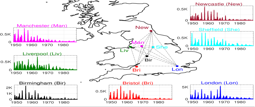
Figure 1: Weekly Reports of Measles and Chickenpox in 7 Major Cities of England and Wales: London (Lon), Bristol (Bri), Liverpool (Liv), Manchester (Man), Newcastle (New), Birmingham (Bir), Sheffield (She)

Symbol(s)	Expression(s)	Definition(s)
${\mathcal{N}}$	$\{1,\dots,N\}$	Set of all the $N$ nodes in the network
$\pi^{i}$	-	Set of potential parents for node $i$
$\kappa_{ij},\theta_{ij}$	-	Gamma distribution hyperparameters for link $ij$
$N_{T},M,N_{B}$	$N_{T}=M\times N_{B}$	Length of observed data, Number of blocks, Length of each block
${\boldsymbol{\gamma}}_{1},{\boldsymbol{\gamma}}_{2}$	${\boldsymbol{\gamma}}_{j}=(\gamma_{j}^{1},\dots,\gamma_{j}^{N})$, $j=1,2$	Hyperparameters of observed data before and after being infected
${\mathbf{B}}_{b}$	$[M(b-1)+1,\dots,Mb]^{T}$	Vector of time indices in block $b$
${\mathbf{d}}_{{\mathbf{B}}_{b}}$	$\{{\mathbf{d}}_{{\mathbf{B}}_{b}}^{1},\dots,{\mathbf{d}}_{{\mathbf{B}}_{b}}^{N}\}$	Set of data received in block $b$
${\mathbf{z}}_{b}$	$[z_{b}^{1},\dots,z_{b}^{N}]^{T}$	Random vector of parents in block $b$
${\mathbf{t}}_{b}$	$[t_{b}^{1},\dots,t_{b}^{N}]^{T}$	Random vector of infection times in block $b$
${\boldsymbol{\alpha}}_{b}$	$[\alpha_{b}^{1},\dots,\alpha_{b}^{N}]^{T}$	Random matrix of link strengths in block $b$
${\mathbf{x}}_{b}$	$({\mathbf{z}}_{b},{\mathbf{t}}_{b},{\boldsymbol{\alpha}}_{b})$	Infection parameters in block $b$
$p_{b}^{i}$	$1-e^{-\alpha_{b}^{iz_{b}^{i}}}$	Parameter of geometric distribution in block $b$
${\mathbf{x}}_{b}^{MAP}$	$(\hat{{\mathbf{z}}}_{b},\hat{{\mathbf{t}}}_{b},\hat{{\boldsymbol{\alpha}}}_{b})$	MAP estimates of infection parameters in block $b$
${\mathcal{C}}_{b}^{i}$	$\{k|z_{b}^{k}=i\}$	Set of node $i$’s children in block $b$
$\pi_{b}^{i}$	$\{k|k\in\pi^{i},t_{b}^{k}\neq\phi,t_{b}^{k}<t_{b}^{i}\}$	Set of node $i$’s potential parents in block $b$
${\mathbf{z}}_{b}^{\overline{i}}$	$[z_{b}^{1},\dots,z_{b}^{i-1},z_{b}^{i+1},\dots,z_{b}^{N}]^{T}$	Vector of parents except node $i$ in block $b$
${\mathbf{t}}_{b}^{\overline{i}}$	$[t_{b}^{1},\dots,t_{b}^{i-1},t_{b}^{i+1},\dots,t_{b}^{N}]^{T}$	Vector of infection times except node $i$ in block $b$
${\boldsymbol{\alpha}}_{b}^{\overline{ij}}$	$[\alpha_{b}^{i1},\dots,\alpha_{b}^{i(j-1)},\alpha_{b}^{i(j+1)},\dots,\alpha_{b}^{iN}]^{T}$	Vector of node $i$’s link strengths except for link $ij$ in block $b$
${\mathbf{x}}_{b}^{m}$	$({\mathbf{z}}_{b}^{m},{\mathbf{t}}_{b}^{m},{\boldsymbol{\alpha}}_{b}^{m})$	The $m^{\text{th}}$ sample from the distribution $f({\mathbf{x}}_{b}|{\mathbf{d}}_{{\mathbf{B}}_{1:b}})$ in block $b$
$r_{b}$	-	Geometric parameter in the proposal for infection times in block $b$
${\mathbf{t}}_{b}^{ML}$	$[{t_{b}^{ML}}^{1},\dots,{t_{b}^{ML}}^{N}]^{T}$	Vector of maximum likelihood changepoints of ${\mathbf{d}}_{{\mathbf{B}}_{b}}$
$N_{thin},N_{burn}$	-	Thinning and burn-in factors
$N_{MCMC},N_{s}$	$N_{MCMC}=N_{s}\times N_{thin}+N_{burn}$	Number of generated and stored particles

TABLE I: Summary of Notations Used in the Paper

II Related Work

In this section, we review the existing research most closely related to this paper. We first discuss the studies that assume the cascades (infection times) are perfectly observed and propose methods to infer just the network structure (II-A). Then in II-B, we describe the few existing studies that have the same assumption as this paper and clarify how this paper contributes to this body of literature. The key assumption is that neither the network structure nor the infection times are perfectly or directly observed. In II-C, we survey methods for detecting the moment of time at which the statistical characteristics of multiple time series change. These methods do not involve any notion of an underlying diffusion network that induces relationships between the time series.

II-A Network Inference with Perfect Cascade Observation

Most of the earlier work exploring diffusion network inference techniques assumes that cascades are perfectly observed, i.e., the infection times are exactly known. [4] models diffusion processes as discrete networks of continuous temporal processes occurring at different rates. Given the infection times, the goal is to infer the parental relationships and estimate the link strengths that maximize the likelihood of the observed data. An algorithm called NETRATE is developed to solve the convex optimization problem. [5] uses a tree-shaped graph of the parental relationships inferred from observed cascades of different contagions to infer the complete set of edges of the graph (for example a friendship graph in a social network). The proposed NETINF algorithm is used to find the maximum likelihood graph conditioned on the set of observed cascades.

[10] uses the same setup as [4], but it assumes that the underlying network structure is not static and infection pathways change over time. A stochastic convex optimization is employed to infer the dynamic network and an online inference algorithm called INFOPATH is developed to solve it. [11] studies how the network evolution affects the diffusion process and proposes a joint continuous-time model to account for co-evolutionary dynamics between these two processes.

[12] considers inferring the network structure as an intermediate task and focuses on estimating joint properties of networks and diffusion processes such as the node influence score of a contagion. The network structure (parental relationships and link strengths) is assumed to be hidden and the infection times are observed. A Bayesian framework is used to calculate the expectation of the hidden parameters under the posterior distribution. Instead of inferring the network structure, [2] and [3] focus on the global influence a node has on the rate of diffusion through the network. The authors develop a linear influence model in which the growth in the number of newly infected nodes is expressed as a function of the infection times of the previously infected nodes. [2] shows that the influence function of each node can be estimated using a simple least squares procedure by modelling it in a non-parametric way. [3] uses the same linear influence model, but introduces sparsity in the estimated influence matrix and applies regularization penalties to take into account the nodes’ centralities.

II-B Network Inference without Perfect Cascade Observation

We now review the existing inference techniques for scenarios where cascades are not perfectly observed. Assuming that the infection times are only partially observed and the diffusion trace is incomplete, [13] develops a two-stage framework to pinpoint the infection source. After learning a continuous-time diffusion network model based on the historical diffusion trace in the first stage, the source of an incomplete diffusion trace is identified by maximizing its likelihood under the learned model. Importance sampling approximation is used to find optimal solutions. Using a four state infection model (Susceptible, Exposed, Infected, and Recovered), [8] assumes that partially observed probabilistic information about the state of each node is provided, but the exact state transition times (infection times) are not observed. The underlying network is inferred by minimizing the expected loss over all realizations of the unobservable trace. The loss function is the negative log-likelihood of node state probabilities at each observed time point in a realization of infection times. Although the network structure can be detected using a convex optimization problem, the transition (infection) times are not estimated.

[14] studies the theoretical learnability of tree-like graphs given the initial and final set of infected nodes. The traces are defined as sets of unordered nodes and the authors strive to reconstruct the underlying network. Their proposed algorithm works by observing the relation that a particular vertex’s infection has on the likelihood of infection at other locations in the tree. The goal in [15] is to reconstruct the so-called node couplings using Dynamic Message Passing (DMP) equations. The authors assume that the cascade observations are only partially available and define coupling of nodes $i$ and $j$ as the probability that the infected node $i$ transmits the contagion to its susceptible neighbour $j$.

In this paper, we improve upon these existing methods by proposing an approach to simultaneously infer the structure and cascade trace of a diffusion process when the infection times are completely unavailable. The batch inference approach presented in this paper (see Section IV) was introduced in an earlier conference paper [16], but here we include more extensive experimental results and develop an online version of the inference algorithm.

II-C Changepoint Detection

Another sizeable, related body of literature addresses detecting abrupt changes in the statistical structure of multiple time series. The moments in time that divide time series into distinct homogeneous segments are referred to as changepoints. We refer the reader to [17] for a detailed discussion of the topic.

Most changepoint detection, or time series segmentation, methods strive to detect single and multiple changepoints in univariate [18, 17, 19] or independent multivariate [20] time series. More closely related to our work is the approach in [21], which involves an underlying Gaussian graphical model that captures the correlation structure between multivariate time series. There is no notion of a diffusion process; the model captures contemporaneous correlation structure. In this paper, we strive to detect the changepoints of multiple time series in the context of a background diffusion process that dictates when the changepoints occur. We combine the indications of change in the statistical characteristics of the observed cascades with the causality relationships between nodes to infer the underlying structure as well as the infection times (i.e., the changepoints).

III System Model

We consider a set of $N$ nodes ${\mathcal{N}}=\{1,\dots,N\}$ that are exposed to a contagion $C$. We assume that $C$ originates in a subset of nodes and is transmissible to other nodes of the network. We denote the moment of time at which node $i$ receives the contagion by $t^{i}$. When node $j\in{\mathcal{N}}$ transfers the contagion to node $i\in{\mathcal{N}}$ for the first time, we say $i$ is infected by $j$. In this case, node $j$ is referred to as the parent of node $i$ and is denoted by $z^{i}$. In this paper, we focus on the Susceptible-Infected (SI) scenarios in which an arbitrary node $i$ is infected by the first node that transfers the infection to it and never recovers afterwards. Each node $i$ has a set of potential parents $\pi^{i}$, but it is infected by only one of them i.e. $z^{i}\in\pi^{i}$. The factor that determines which member of $\pi^{i}$ transfers the infection to node $i$ is the strength of the relationship between node $i$ and each of its potential parents $j\in\pi^{i}$. We denote this link strength for nodes $i$ and $j$ by $\alpha^{ij}$. The definitions of parents and candidate parents simply imply that $\forall j\in\pi^{i}:t^{j}<t^{i}$ and $\forall j\notin\pi^{i}:\alpha^{ij}=0$. Now that we have characterized both the diffusion components and the cascades, we assign a directed, weighted graph to the diffusion process. A directed edge $j\rightarrow i$ with weight $\alpha^{ij}$ exists in this graph if and only if $z^{i}=j$ . We denote this graph by $G=({\mathcal{N}},{\mathcal{E}},{\boldsymbol{\alpha}}_{N\times N})$ where ${\mathcal{E}}$ is the set of directed edges, and ${\boldsymbol{\alpha}}=[\alpha^{ij}]_{N\times N}$ is the weight matrix. Throughout the paper, we use $[\cdot]$ to denote vectors and matrices, $\{\cdot\}$ to denote sets, and $(\cdot)$ to denote finite ordered lists.

As mentioned in Section I, we focus on the scenarios where neither the network structure (i.e., parental relations and link strengths) nor the cascades (i.e., infection times) are directly observed. We assume that the only observation we get from an arbitrary node $i\in{\mathcal{N}}$ is a discrete time signal of length $N_{T}$ denoted by ${\mathbf{d}}^{i}=(d^{1}_{n},\dots,d_{n}^{N_{T}})$. We denote the set of all observed time signals by ${\mathbf{d}}=\{{\mathbf{d}}^{1},\dots,{\mathbf{d}}^{N}\}$.

In order to develop inference algorithms for the case where data arrives in a streaming fashion or in batches, we consider a setting where each node’s data arrives in $N_{B}$ blocks of length $M$. Denote the vector of time indices in block $b$ by ${\mathbf{B}}_{b}$ i.e. ${\mathbf{B}}_{b}=[M\times(b-1)+1,\dots,M\times b]^{T}$ and the data in block $b$ for all the nodes in the network by ${\mathbf{d}}_{{\mathbf{B}}_{b}}=\{{\mathbf{d}}_{{\mathbf{B}}_{b}}^{1},\dots,{\mathbf{d}}_{{\mathbf{B}}_{b}}^{N}\}$.

We denote the parent for node $i$ at the end of the $b^{\text{th}}$ block by $z_{b}^{i}$. If no infection has occurred by the end of block $b-1$, but it occurs during the $b^{\text{th}}$ block, then $z_{b-1}^{i}$ has a null-value, i.e., $z_{b-1}^{i}=\phi$, whereas $z_{b}^{i}=j$ for some $j\in\pi_{i}$. Likewise, the infection time for node $i$ and the link strength associated with link $ij$ in block $b$ are respectively denoted by $t_{b}^{i}$ and $\alpha_{b}^{ij}$. If no infection has occurred then $t_{b}^{i}$ also has a null-value $\phi$.

The parameters at the end of the $b^{\text{th}}$ block are denoted by ${\mathbf{x}}_{b}=({\mathbf{z}}_{b},{\mathbf{t}}_{b},{\boldsymbol{\alpha}}_{b})$ where ${\mathbf{z}}_{b}=[z_{b}^{1},\dots,z_{b}^{N}]^{T}$, ${\mathbf{t}}_{b}=[t_{b}^{1},\dots,t_{b}^{N}]^{T}$, and ${\boldsymbol{\alpha}}_{b}=[\alpha_{b}^{ij}]_{N\times N}$. While the set of potential parents $\pi^{i}$ is the same for all the blocks, two sets ${\mathcal{C}}_{b}^{i}$ and $\pi_{b}^{i}$ are defined as follows for each block $b$.

$${\mathcal{C}}^{i}_{b}=\{k|z_{b}^{k}=i\}\quad,\quad\pi_{b}^{i}=\{k|k\in\pi^{i},t_{b}^{k}\neq\phi,t_{b}^{k}<t_{b}^{i}\}$$

$\mathcal{C}_{b}^{i}$ is the set of nodes that node $i$ has infected before the end of the $b^{\text{th}}$ block, i.e., node $i$ is the established parent of all nodes $j\in\mathcal{C}_{b}^{i}$. $\pi_{b}^{i}\subseteq\pi^{i}$ is the subset of potential parents of node $i$ who have been infected by the end of the $b^{\text{th}}$ block. Table I lists the notation used in this paper. The goal is to infer the set of infection parameters ${\mathbf{x}}_{b}$ at the end of the $b^{\text{th}}$ block that best explains the received signals up to the end of block $b$, i.e., ${\mathbf{d}}_{{\mathbf{B}}_{1:b}}=\{{\mathbf{d}}_{{\mathbf{B}}_{1}},...,{\mathbf{d}}_{{\mathbf{B}}_{b}}\}$. More precisely, we aim to find the most probable set of parameters $(\hat{{\mathbf{z}}}_{b},\hat{{\mathbf{t}}}_{b},\hat{{\boldsymbol{\alpha}}}_{b})$ conditioned on the received signals ${\mathbf{d}}_{{\mathbf{B}}_{1:b}}$. We denote this set of Maximum A Posteriori (MAP) estimate of infection parameters by ${\mathbf{x}}^{MAP}_{b}$:

$${\mathbf{x}}^{MAP}_{b}=(\hat{{\mathbf{z}}}_{b},\hat{{\mathbf{t}}}_{b},\hat{{\boldsymbol{\alpha}}}_{b})=\underset{({\mathbf{z}}_{b},{\mathbf{t}}_{b},{\boldsymbol{\alpha}}_{b})}{\arg\max}\quad f({\mathbf{z}}_{b},{\mathbf{t}}_{b},{\boldsymbol{\alpha}}_{b}|{\mathbf{d}}_{{\mathbf{B}}_{1:b}})$$ (1)

Solving the optimization problem in (1) is challenging, especially considering the fact that the data arrives in blocks and we need to make decisions before we have access to the entire signals. Hence, we resort to Monte Carlo Markov Chain (MCMC) methods to generate samples from the posterior distribution, $f({\mathbf{z}}_{b},{\mathbf{t}}_{b},{\boldsymbol{\alpha}}_{b}|{\mathbf{d}}_{{\mathbf{B}}_{1:b}})$, and assess the underlying diffusion process based on these samples. We first describe the batch inference approach based on Gibbs Sampling (GS) that we proposed in [16]. We then extend this framework by considering the cases where no infection time is detected in the interval under study. We use this batch inference method to generate particles in the first received block of data. We then design an online inference algorithm based on Sequential Monte Carlo (SMC) techniques to find the set of infection parameters (i.e. network structure and cascade information) that best explains the observed data at the end of each block $b>1$. In order to do so, the particles for each block $b$ are obtained by updating particles of block $b-1$ using the received signals ${\mathbf{d}}_{{\mathbf{B}}_{b}}$. In order to have a unified notation throughout the paper, we use the $b$ batch sub-indices from now on for both the batch and sequential settings. For batch inference scenarios we have ${\mathbf{x}}={\mathbf{x}}_{1}=({\mathbf{z}}_{1},{\mathbf{t}}_{1},{\boldsymbol{\alpha}}_{1})$ since $N_{B}=1$ and $M=N_{T}$.

IV Batch Inference Method

Assuming that the entire data signal is available at each node, we develop a batch (offline) inference algorithm based on Gibbs Sampling. Using Bayes’ rule and due to the dependencies we clarified in Section III, the joint conditional distribution $f({\mathbf{x}}_{1}|{\mathbf{d}}_{{\mathbf{B}}_{1}})=f({\mathbf{z}}_{1},{\mathbf{t}}_{1},{\boldsymbol{\alpha}}_{1}|{\mathbf{d}}_{{\mathbf{B}}_{1}})$ is

$$f({\mathbf{x}}_{1}|{\mathbf{d}}_{{\mathbf{B}}_{1}})=\frac{f({\mathbf{d}}_{{\mathbf{B}}_{1}}|{\mathbf{t}}_{1},{\mathbf{z}}_{1},{\boldsymbol{\alpha}}_{1})f({\mathbf{t}}_{1}|{\mathbf{z}}_{1},{\boldsymbol{\alpha}}_{1})f({\mathbf{z}}_{1}|{\boldsymbol{\alpha}}_{1})f({\boldsymbol{\alpha}}_{1})}{f({\mathbf{d}}_{{\mathbf{B}}_{1}})}$$ (2)

In the rest of this section, we introduce appropriate prior distributions for components of equation (2). The priors are selected to allow flexibility in the incorporation of prior knowledge and to facilitate computation. We then use this Bayesian framework to develop methods for inferring the underlying network structure as well as the cascade traces.

IV-A Priors

As opposed to the previous methods and models (e.g. [4, 12, 16]), we accommodate scenarios where an arbitrary node $i$ may never become infected over the study period of length $N_{T}$. We indicate this case by assigning null values to the infection time and parent of node $i$, i.e., $t_{1}^{i}=\phi$ and $z_{1}^{i}=\phi$. The main building block of the diffusion model is the probability density function $f(t_{1}^{i}|z_{1}^{i},\alpha_{1}^{iz^{i}},t_{1}^{z^{i}})$, which models the conditional likelihood that node $z_{1}^{i}$ (infected at time $t_{1}^{z_{1}^{i}}$) transfers the infection to node $i$ at time $t_{1}^{i}>t_{1}^{z_{1}^{i}}$. Intuitively, the ability of an infected node to transfer the contagion to other nodes is expected to decay as time passes. Hence, the monotonic memoryless exponential distribution is a good candidate. An alternative way to motivate this model is to consider repeated interactions between the nodes, each being a Bernoulli trial with a small probability of infection.

Some authors (e.g. [4]) have studied the effect of heavy tailed Power law or non-monotonic Rayleigh distributions on the inference methods when the cascades are observed. For our prior distribution, we employ the exponential decay assumption. Since our observations ${\mathbf{d}}$ are assumed to be discrete time series, we choose the discrete counterpart of an exponential distribution for $f(t_{1}^{i}|z_{1}^{i},\alpha_{1}^{iz_{1}^{i}},t_{1}^{z_{1}^{i}})$, i.e., a geometric distribution with parameter $p_{1}^{i}=1-e^{-\alpha_{1}^{iz_{1}^{i}}}$.

Consider the case where $t_{1}^{1}\geq t_{1}^{2}\geq\dots\geq t_{1}^{N}$, employing the convention that the null infection time $\phi>N_{T}$. We have $f({\mathbf{t}}_{1}|{\mathbf{z}}_{1},{\boldsymbol{\alpha}}_{1})=\prod_{i\in{\mathcal{N}}}f(t_{1}^{i}|z_{1}^{i},{\boldsymbol{\alpha}}_{1},t_{1}^{i+1:N})$ where

$$f(t_{1}^{i}|z_{1}^{i},{\boldsymbol{\alpha}}_{1},t_{1}^{i+1:N})=\begin{cases}p_{1}^{i}(1-p_{1}^{i})^{t_{1}^{i}-t_{1}^{z_{1}^{i}}-1}&1\leq t_{1}^{i}\leq N_{T},\\ (1-p_{1}^{i})^{N_{T}}&\quad t_{1}^{i}=\phi.\end{cases}$$ (3)

The expression for $t_{1}^{i}=\phi$ is simply one minus the value of the cumulative distribution function of the random variable $t_{1}^{i}$ at time $N_{T}$. A similar expression can be obtained for any arbitrary ordering of the changepoints.

We assume that, conditioned on the link strengths, the probability that one of the nodes in the candidate parent set $v\in\pi_{i}$ is the actual parent $z_{i}$ of node $i$ is independent of the probability that a node $r\in\pi_{j}$ is the parent $z_{j}$ of node $j$. The exponential decay assumption and the fact that $z_{1}^{i}$ is the first node that transfers the infection to node $i$ makes the multinomial distribution a good candidate for capturing the prior distribution of parents given the link strength values:

$$f({\mathbf{z}}_{1}|{\boldsymbol{\alpha}}_{1})=\prod_{i\in{\mathcal{N}}}f(z_{1}^{i}|\alpha_{1}^{ij},{j\in\pi^{i}})=\prod_{i\in{\mathcal{N}}}\frac{\alpha_{1}^{iz_{1}^{i}}}{\sum_{j\in\pi^{i}}\alpha_{1}^{ij}}$$ (4)

As for the prior distribution for strength value of link $ij$, we choose a Gamma distribution, i.e., $\alpha_{1}^{ij}\sim\Gamma(\kappa_{ij},\theta_{ij})$. This choice of prior distribution allows us to model a wide range of $\alpha$ values for different links of the network. We can capture both highly informed knowledge about strong links or the uninformed case where we have little prior information about the strength of links. Therefore, assuming that link strength values of different links are independent, we have

$$f({\boldsymbol{\alpha}}_{1})=\prod_{i\in{\mathcal{N}},j\in\pi^{i}}f(\alpha_{1}^{ij})=\prod_{i\in{\mathcal{N}},j\in\pi^{i}}\frac{x^{\kappa_{ij}-1}e^{-\frac{x}{\theta_{ij}}}}{\Gamma(\kappa_{ij}){\theta_{ij}}^{\kappa_{ij}}}$$ (5)

Finally, we assume that node $i$’s observed data, ${\mathbf{d}}_{{\mathbf{B}}_{1}}^{i}$, are conditionally independent of the observations from all other nodes and that they follow the same prior distribution with two different sets of hyperparameters ${\boldsymbol{\gamma}}_{1}=(\gamma_{1}^{1},\dots,\gamma_{1}^{N})$, ${\boldsymbol{\gamma}}_{2}=(\gamma_{2}^{1},\dots,\gamma_{2}^{N})$ before and after being infected at $t^{i}$. Hence,

$$f({\mathbf{d}}_{{\mathbf{B}}_{1}}|{\mathbf{z}}_{1},{\mathbf{t}}_{1},{\boldsymbol{\alpha}}_{1}) =\prod_{i\in{\mathcal{N}}}f({\mathbf{d}}_{{\mathbf{B}}_{1}}^{i}|t_{1}^{i})$$ (6)

$$=\prod_{i\in{\mathcal{N}}}f(d^{i}_{1:t^{i}};\gamma_{1}^{i})f(d^{i}_{t^{i+1}:N_{T}};\gamma_{2}^{i})$$

The choice of prior $f(d^{i}_{1:t^{i}};\gamma_{1}^{i})$ depends on the application. We test cases where the data are independently drawn from Gaussian and Poisson distributions in our numerical simulations in Section VI, but more complex structure can be readily incorporated in the time-series model (autoregressive processes, for example). In the next section, we use the prior distributions described above to design batch and online inference methods in a Bayesian framework.

IV-B Gibbs Sampling

With the proposed distributions in (3)-(6), we can calculate the probability of any arbitrary set $({\mathbf{z}}_{1},{\mathbf{t}}_{1},{\boldsymbol{\alpha}}_{1})$ up to a constant $\frac{1}{f({\mathbf{d}}_{{\mathbf{B}}_{1}})}$ using (2). We use Gibbs Sampling (GS) to generate $N_{s}$ samples from the posterior distribution of (2). In other words, we use full conditional distributions for each of the infection parameters $z_{1}^{i},t_{1}^{i},\alpha_{1}^{ij}$ ($i,j\in{\mathcal{N}}$) to generate samples. We denote the parents and infection times of all the nodes in the network except node $i$ respectively by ${\mathbf{z}}_{1}^{\overline{i}}$, ${\mathbf{t}}_{1}^{\overline{i}}$. Also, the vector of link strengths of all node $i$’s links except the link between nodes $i$ and $j$ is denoted by ${\boldsymbol{\alpha}}_{1}^{\overline{ij}}$ . The full conditional probabilities for GS are as follows.

a) For the parent of node $i\in{\mathcal{N}}$

$$f(z_{1}^{i}|{\mathbf{d}}_{{\mathbf{B}}_{1}},{\mathbf{z}}_{1}^{\overline{i}},{\mathbf{t}}_{1},{\boldsymbol{\alpha}}_{1})\propto f(t_{1}^{i}|z_{1}^{i},\alpha_{1}^{iz_{1}^{i}},t_{1}^{z_{1}^{i}})f(z_{1}^{i}|\alpha_{1}^{ij})_{j\in\pi^{i}}$$ (7)

b) For the infection time of node $i\in{\mathcal{N}}$

$$f(t_{1}^{i}|{\mathbf{d}}_{{\mathbf{B}}_{1}},{\mathbf{z}}_{1}, {\mathbf{t}}_{1}^{\overline{i}},{\boldsymbol{\alpha}}_{1})\propto$$ (8)

$$f({\mathbf{d}}_{{\mathbf{B}}_{1}}^{i}|t_{1}^{i})f(t_{1}^{i}|z_{1}^{i},\alpha_{1}^{iz_{1}^{i}},t_{1}^{z_{1}^{i}})\prod_{k\in{\mathcal{C}}_{1}^{i}}f(t_{1}^{k}|\alpha_{1}^{ki},t_{1}^{i})$$

c) For the link strength between nodes $i\in{\mathcal{N}}$ and $j\in\pi^{i}$

$$f(\alpha_{1}^{ij}|{\mathbf{d}}_{{\mathbf{B}}_{1}},{\mathbf{z}}_{1},{\mathbf{t}}_{1},{\boldsymbol{\alpha}}^{\overline{ij}}_{1})\propto f(t_{1}^{i}|z_{1}^{i},\alpha_{1}^{iz_{1}^{i}},t_{1}^{z_{1}^{i}})f(z_{1}^{i}|{\boldsymbol{\alpha}}_{1})f(\alpha_{1}^{ij})$$ (9)

Building upon this batch inference method, we propose an online inference method in the next section. In this online approach, the batch inference method is used to make decisions about diffusion parameters in the first received block of data.

V Online Inference Method

In the online setting, the goal is to compute the filtering posterior distribution $f({\mathbf{x}}_{b}|{\mathbf{d}}_{{\mathbf{B}}_{1:b}})$. In the Bayesian framework we have,

$$f({\mathbf{x}}_{b}|{\mathbf{d}}_{{\mathbf{B}}_{1:b}})\propto\int f({\mathbf{d}}_{{\mathbf{B}}_{b}}|{\mathbf{x}}_{b})f({\mathbf{x}}_{b}|{\mathbf{x}}_{b-1})f({\mathbf{x}}_{b-1}|{\mathbf{d}}_{{\mathbf{B}}_{1:b-1}})d_{{\mathbf{x}}_{b-1}}$$ (10)

Since calculating (10) is analytically intractable in our application, we use the sequential Markov Chain Monte Carlo (SMCMC) framework proposed in [22] to obtain an approximation of this filtering distribution. In this framework, instead of striving to directly sample from $f({\mathbf{x}}_{b}|{\mathbf{d}}_{{\mathbf{B}}_{1:b}})$, which has complexity issues due to the need to perform the marginalization captured by the integral in (10), we sample from the joint posterior distribution $f({\mathbf{x}}_{b},{\mathbf{x}}_{b-1}|{\mathbf{d}}_{{\mathbf{B}}_{1:b}})$ where

$$f({\mathbf{x}}_{b},{\mathbf{x}}_{b-1}|{\mathbf{d}}_{{\mathbf{B}}_{1:b}})=\frac{f({\mathbf{d}}_{{\mathbf{B}}_{b}}|{\mathbf{x}}_{b})f({\mathbf{x}}_{b}|{\mathbf{x}}_{b-1})f({\mathbf{x}}_{b-1}|{\mathbf{d}}_{{\mathbf{B}}_{1:b-1}})}{f({\mathbf{d}}_{{\mathbf{B}}_{b}}|{\mathbf{d}}_{{\mathbf{B}}_{1:b-1}})}$$ (11)

In the sequential MCMC approach, we maintain a set of particles that provides a sample-based approximation to the distribution of interest $f({\mathbf{x}}_{b}|{\mathbf{d}}_{{\mathbf{B}}_{1:b}})$. After processing block $b-1$, since the posterior distribution $f({\mathbf{x}}_{b-1}|{\mathbf{d}}_{{\mathbf{B}}_{1:b-1}})$ does not have a closed form representation, it is approximated with an empirical distribution based on the particle set $\{{\mathbf{x}}_{b-1}^{j}|j=1,\dots,N_{s}\}$:

$$f({\mathbf{x}}_{b-1}|{\mathbf{d}}_{{\mathbf{B}}_{1:b-1}})=\frac{1}{N_{s}}\sum_{j=1}^{N_{s}}\delta({\mathbf{x}}_{b-1}-{\mathbf{x}}_{b-1}^{j})$$ (12)

Hence, the target distribution $f({\mathbf{x}}_{b},{\mathbf{x}}_{b-1}|{\mathbf{d}}_{{\mathbf{B}}_{1:b}})$ that we wish to sample from can be approximated as

$$\begin{cases}\frac{f({\mathbf{d}}_{{\mathbf{B}}_{b}}|{\mathbf{x}}_{b})f({\mathbf{x}}_{b}|{\mathbf{x}}_{b-1}^{s})}{\sum_{j=1}^{N_{s}}f({\mathbf{d}}_{{\mathbf{B}}_{b}}|{\mathbf{x}}_{b-1}^{j})}&\text{if }{\mathbf{x}}_{b-1}\in\{{\mathbf{x}}_{b-1}^{s}|s=1,\dots,N_{s}\},\\ 0&\text{otherwise}.\end{cases}$$ (13)

Here, $f({\mathbf{x}}_{b}|{\mathbf{x}}_{b-1}^{s})$ is referred to as the transition distribution. We will derive an appropriate expression for this probability distribution in Section V-A.

Algorithm 1 presents our proposed online inference method based on the MCMC-based particle algorithm used in [22]. As mentioned earlier, we use the batch inference method described in section IV to generate a set of $N_{s}$ particles in the first block of the data and use it as the initial particle set for the SMC procedure of next blocks. In each block $b>1$ of the data, the SMC procedure consists of two main steps. The first step, joint draw, is a joint Metropolis-Hastings (MH) proposal step in which instead of sampling from $f({\mathbf{x}}_{b},{\mathbf{x}}_{b-1}|{\mathbf{d}}_{{\mathbf{B}}_{1:b}})$, we sample from the proposal distribution $q({\mathbf{x}}_{b},{\mathbf{x}}_{b-1}|{\mathbf{x}}_{b}^{m-1},{\mathbf{x}}_{b-1}^{m-1})$ and accept the proposed samples with probability $\rho$. Lines 11-13 of Algorithm 1 describe the components of the proposal distributions. The proposal distributions and the MH acceptance ratio are respectively derived in V-B and V-C. The second step of the SMC procedure, refinement, is an individual refinement GS step where ${\mathbf{x}}_{b}$ is updated by sampling from $f({\mathbf{x}}_{b}|{\mathbf{x}}_{b-1}^{m},{\mathbf{d}}_{{\mathbf{B}}_{b}})$.

Algorithm 1 SMC-Based Online Inference Method

1:  // First block

2:  Generate $N_{s}$ samples ${\mathbf{x}}_{1}^{s}|_{s=1,\dots,N_{s}}\sim f({\mathbf{x}}_{1}|{\mathbf{d}}_{{\mathbf{B}}_{1}})$ using GS

3:  // Next blocks

4:  Initialize the particle set ${\mathcal{P}}=\{{\mathbf{x}}_{1}^{s}|s=1,\dots,N_{s}\}$

5:  Set $N_{MCMC}=N_{thin}\times N_{s}+N_{burn}$

6:  for $b=2,\dots,N_{b}$ do

7:     Calculate ${\mathbf{t}}_{b}^{ML}$ using (19)

8:     for $m=1,\dots,N_{MCMC}$ do

9:        // Joint Draw

10:        Propose ${\mathbf{x}}_{b-1}^{*}$ uniformly from ${\mathcal{P}}$

11:        Propose ${\mathbf{t}}_{b}^{*}\sim h_{{\mathbf{t}}}({\mathbf{t}}_{b}|{\mathbf{x}}_{b-1}^{*};{\mathbf{t}}_{b}^{ML})$ using (22)

12:        Propose ${\boldsymbol{\alpha}}_{b}^{*}\sim h_{{\boldsymbol{\alpha}}}({\boldsymbol{\alpha}}_{b}|{\mathbf{x}}_{b-1}^{*},{\mathbf{t}}_{b}^{*})$ using (24)

13:        Propose ${\mathbf{z}}_{b}^{*}\sim h_{{\mathbf{z}}}({\mathbf{z}}_{b}|{\mathbf{x}}_{b-1}^{*},{\mathbf{t}}_{b}^{*},{\boldsymbol{\alpha}}_{b}^{*})$ using (25)

14:        Set ${\mathbf{x}}_{b}^{*}=({\mathbf{z}}_{b}^{*},{\mathbf{t}}_{b}^{*},{\boldsymbol{\alpha}}_{b}^{*})$

15:        Calculate MH acceptance probability $\rho$ using (28)

16:        Accept $({\mathbf{x}}_{b}^{m},{\mathbf{x}}_{b-1}^{m})=({\mathbf{x}}_{b}^{*},{\mathbf{x}}_{b-1}^{*})$ with probability $\rho$

17:        // Refinement

18:        Generate ${\mathbf{x}}_{b}^{*}\sim f({\mathbf{x}}_{b}|{\mathbf{x}}_{b-1}^{m},{\mathbf{d}}_{{\mathbf{B}}_{b}})$ using GS and set ${\mathbf{x}}_{b}^{m}={\mathbf{x}}_{b}^{*}$

19:     end for

20:     Set ${\mathcal{P}}=\{{\mathbf{x}}_{b}^{N_{burn}+kN_{thin}}|k=1,\dots,N_{s}\}$

21:     Set ${\mathbf{x}}_{b}^{MAP}$ as the most repeated particle in ${\mathcal{P}}$

22:  end for

Finally, thinning and burn-in procedures are performed by storing one out of every $N_{thin}$ accepted samples after discarding the initial $N_{burn}$ samples. In the rest of this section, we derive the transition and proposal distributions and use them to calculate the MH acceptance ratio. We then explain the details of the refinement step and conclude the section by commenting on the computational complexity of Algorithm 1.

V-A Transition Distribution

Using the framework explained in Section III, we have

$$f({\mathbf{x}}_{b}|{\mathbf{x}}_{b-1}^{s}) =f({\mathbf{z}}_{b},{\mathbf{t}}_{b}|{\mathbf{x}}_{b-1}^{s},{\boldsymbol{\alpha}}_{b})f({\boldsymbol{\alpha}}_{b}|{\mathbf{x}}_{b-1}^{s})$$ (14)

$$=\prod_{i\in{\mathcal{N}}}f(t_{b}^{i},z_{b}^{i}|{\mathbf{x}}_{b-1}^{s},{\boldsymbol{\alpha}}_{b})\prod_{k\in\pi^{i}}f(\alpha_{b}^{ik})$$

Due to the characteristics of the online method, once a non-null value has been assigned to the infection parameters of a node in block $b$, this decision is respected in the following blocks. More precisely,

$$f(\alpha_{b}^{ik})=\begin{cases}\delta(\alpha_{b}^{ik}-\alpha_{b-1}^{ik})&\text{if }t_{b-1}^{i}\neq\phi,\\ \Gamma(\kappa_{ik},\theta_{ik})&\text{if }t_{b-1}^{i}=\phi,\end{cases}$$ (15)

and

$$f(t_{b}^{i},z_{b}^{i}|{\mathbf{x}}_{b-1}^{s},\alpha_{b}^{ij})_{j\in\pi_{b}^{i}}=$$ (16)

$$\begin{cases}\delta(t_{b}^{i}-t_{b-1}^{i})\delta(z_{b}^{i}-z_{b-1}^{i})&\text{if }t_{b-1}^{i}\neq\phi,\vspace{0.2cm}\\ \begin{tabular}[]{@{}c@{}}$\sum_{l\in\pi_{b}^{i}}\sum_{x=t_{b}^{l}+1}^{{\mathbf{B}}_{b}[M]}g_{1}(l,x,i)+\delta(z_{b}^{i}-\phi)\times$\\ $\delta(t_{b}^{i}-\phi)(1-\sum_{l\in\pi_{b}^{i}}\sum_{x=t_{b}^{l}+1}^{{\mathbf{B}}_{b}[M]}g_{1}(l,x,i))$\end{tabular}&\text{if }t_{b-1}^{i}=\phi,\end{cases}$$

where

$$g_{1}(l,x,i)=\frac{\alpha_{b}^{il}}{\sum_{k\in\pi^{i}}\alpha_{b}^{ik}}(p_{b}^{i})(1-p_{b}^{i})^{x-t_{b}^{l}-1}\delta(z_{b}^{i}-l)\delta(t_{b}^{i}-x)$$ (17)

and $p_{b}^{i}=1-e^{-\alpha_{b}^{iz_{b}^{i}}}$. According to (16), if node $i$ has not become infected by the end of block $b-1$, the probability that it becomes infected by node $l\in\pi_{b}^{i}$ at some time $x\in[t_{b}^{l},{\mathbf{B}}_{b}[M]]$ is $g_{1}(l,x,i)$. Equation (17) shows that this probability equals the product of the geometric and multinomial distributions respectively defined in (3) and (4). Node $i$ remains susceptible (i.e., $t_{b}^{i}=\phi$) with a probability that equals one minus the sum of the probabilities of being infected by each node $l\in\pi_{i}$ at each time step $x\in[t_{b}^{l},{\mathbf{B}}_{b}[M]]$.

V-B Proposal Distribution

As presented in line 9 of Algorithm 1, the optimal importance sampling distribution (assuming that we adopt the particle-based approximation for $f({\mathbf{x}}_{b-1}|{\mathbf{d}}_{{\mathbf{B}}_{1:b-1}})$) is:

$$q({\mathbf{x}}_{b},{\mathbf{x}}_{b-1}|{\mathbf{x}}_{b}^{m-1},{\mathbf{x}}_{b-1}^{m-1})=f({\mathbf{x}}_{b}|{\mathbf{x}}_{b-1},{\mathbf{d}}_{{\mathbf{B}}_{b}})f({\mathbf{x}}_{b-1}|{\mathbf{d}}_{{\mathbf{B}}_{1:b-1}})$$ (18)

$$=\begin{cases}\frac{f({\mathbf{d}}_{{\mathbf{B}}_{b}}|{\mathbf{x}}_{b})f({\mathbf{x}}_{b}|{\mathbf{x}}_{b-1})}{f({\mathbf{d}}_{{\mathbf{B}}_{b}}|{\mathbf{x}}_{b-1})}&\text{if }{\mathbf{x}}_{b-1}\in\{{\mathbf{x}}_{b-1}^{s},s=1,\dots,N_{s}\},\\ 0&\text{otherwise}.\end{cases}$$

Although calculating the predictive density in the denominator of (18) is not necessary for sampling, it is eventually required for calculating the acceptance ratio. To avoid numerical integration of the predictive density at every iteration, we benefit from an auxiliary parameter which can be obtained from the data. In each block $b$, we calculate the maximum likelihood changepoint of each individual time series ${\mathbf{d}}_{{\mathbf{B}}_{b}[1]:{\mathbf{B}}_{b}[M]}$ for all $i\in{\mathcal{N}}$. We denote the vector of these maximum likelihood changepoints by ${\mathbf{t}}_{b}^{ML}=[t_{b}^{ML^{1}},\dots,t_{b}^{ML^{N}}]^{T}$, where

$$t_{b}^{ML^{i}}\triangleq\arg\underset{{\mathbf{B}}_{b}[1]\leq t\leq{\mathbf{B}}_{b}[M]}{\max}f({\mathbf{d}}_{{\mathbf{B}}_{b}[1]:t};\gamma_{1}^{i})f({\mathbf{d}}_{t+1:{\mathbf{B}}_{b}[M]};\gamma_{2}^{i})$$ (19)

Using this auxiliary parameter, we design the following proposal distribution.

$$q({\mathbf{x}}_{b},{\mathbf{x}}_{b-1}|{\mathbf{x}}_{b}^{m-1},{\mathbf{x}}_{b-1}^{m-1})=h({\mathbf{x}}_{b}|{\mathbf{x}}_{b-1};{\mathbf{t}}_{b}^{ML})f({\mathbf{x}}_{b-1}|{\mathbf{d}}_{{\mathbf{B}}_{1:b-1}})$$ (20)

$$=\begin{cases}\frac{1}{N_{s}}h({\mathbf{x}}_{b}|{\mathbf{x}}_{b-1};{\mathbf{t}}_{b}^{ML})&\text{if }{\mathbf{x}}_{b-1}\in\{{\mathbf{x}}_{b-1}^{s},s=1,\dots,N_{s}\},\\ 0&\text{otherwise}.\end{cases}$$

where

$$h({\mathbf{x}}_{b}|{\mathbf{x}}_{b-1};{\mathbf{t}}_{b}^{ML})=$$ (21)

$$h_{{\mathbf{t}}}({\mathbf{t}}_{b}|{\mathbf{x}}_{b-1};{\mathbf{t}}_{b}^{ML})h_{{\boldsymbol{\alpha}}}({\boldsymbol{\alpha}}_{b}|{\mathbf{t}}_{b},{\mathbf{x}}_{b-1})h_{{\mathbf{z}}}({\mathbf{z}}_{b}|{\mathbf{t}}_{b},{\boldsymbol{\alpha}}_{b},{\mathbf{x}}_{b-1}).$$

Each component of $h({\mathbf{x}}_{b}|{\mathbf{x}}_{b-1};{\mathbf{t}}_{b}^{ML})$ is the proposal distribution for one of the infection parameters. For each node $i\in{\mathcal{N}}$, we independently propose an infection time whose distance from the maximum likelihood $t_{b}^{ML^{i}}$ follows a geometric distribution with pre-defined parameter $r_{b}^{i}$. In other words, we sample from $h_{{\mathbf{t}}}({\mathbf{t}}_{b}|{\mathbf{x}}_{b-1};{\mathbf{t}}_{b}^{ML})=\prod_{i\in{\mathcal{N}}}h_{t}^{i}(t_{b}^{i}|{\mathbf{x}}_{b-1};t_{b}^{ML^{i}})$, where

$$h_{t}^{i}(t_{b}^{i}|{\mathbf{x}}_{b-1};t_{b}^{ML^{i}})=$$ (22)

$$\begin{cases}\delta(t_{b}^{i}-t_{b-1}^{i})&t_{b-1}^{i}\neq\phi,\\ \sum_{n=1}^{M}g_{2}(n,i)+(1-\sum_{n=1}^{M}g_{2}(n,i))\delta(t_{b}^{i}-\phi)&t_{b-1}^{i}=\phi.\end{cases}$$

and

$$g_{2}(n,i)=\frac{1}{2}r_{b}^{i}(1-r_{b}^{i})^{|{\mathbf{B}}_{b}[n]-t_{b}^{ML^{i}}|}\delta(t_{b}^{i}-{\mathbf{B}}_{b}[n]).$$ (23)

Using the proposed ${\mathbf{t}}_{b}^{*}$, we propose ${\boldsymbol{\alpha}}_{b}^{*}$ by sampling from $h_{{\boldsymbol{\alpha}}}({\boldsymbol{\alpha}}_{b}|{\mathbf{t}}_{b}^{*},{\mathbf{x}}_{b-1})=\prod_{i\in{\mathcal{N}}}\prod_{k\in\pi^{i}}h_{\alpha}^{i}(\alpha_{b}^{ik}|{\mathbf{t}}_{b}^{*},{\mathbf{x}}_{b-1})$ where

$$h_{\alpha}^{i}(\alpha_{b}^{ik}|{\mathbf{t}}_{b}^{*},{\mathbf{x}}_{b-1})=\begin{cases}\delta(\alpha_{b}^{ik}-\alpha_{b-1}^{ik})&\text{if }t_{b}^{i}\neq\phi,t_{b-1}^{i}\neq\phi,\\ \Gamma(\kappa_{ki},\theta_{ki})&\text{if }t_{b-1}^{i}=\phi.\end{cases}$$ (24)

Finally, we propose ${\mathbf{z}}_{b}^{*}$ by generating samples from $h_{{\mathbf{z}}}({\mathbf{z}}_{b}|{\mathbf{t}}_{b}^{*},{\boldsymbol{\alpha}}_{b}^{*},{\mathbf{x}}_{b-1})=\prod_{i\in{\mathcal{N}}}h_{z}^{i}(z_{b}^{i}|{\mathbf{t}}_{b}^{*},{\boldsymbol{\alpha}}_{b}^{*},{\mathbf{x}}_{b-1})$, i.e.,

$$h_{z}^{i}(z_{b}^{i}|{\mathbf{t}}_{b}^{*},{\boldsymbol{\alpha}}_{b}^{*},{\mathbf{x}}_{b-1})=$$ (25)

$$\begin{cases}\delta(z_{b}^{i}-z_{b-1}^{i})&\text{if }t_{b}^{i}\neq\phi,t_{b-1}^{i}\neq\phi,\\ \delta(z_{b}^{i}-\phi)&\text{if }t_{b}^{i}=\phi,t_{b-1}^{i}=\phi,\\ \begin{tabular}[]{@{}c@{}}$\sum_{l\in\pi_{b}^{i}}\frac{\alpha_{b}^{il}}{\sum_{j\in\pi^{i}}\alpha_{b}^{ij}}\delta(z_{b}^{i}-l)$+\\ $(1-\frac{\sum_{l\in\pi_{b}^{i}}\alpha_{b}^{il}}{\sum_{j\in\pi^{i}}\alpha_{b}^{ij}})\delta(z_{b}^{i}-\phi)$\end{tabular}&\text{if }t_{b}^{i}\neq\phi,t_{b-1}^{i}=\phi.\end{cases}$$

Proposition 1 shows that the proposal $q$ is normalized. The proof is provided in Appendix A.

Proposition 1.

$h({\mathbf{x}}_{b}|{\mathbf{x}}_{b-1};{\mathbf{t}}_{b}^{ML})$ is a probability distribution function. In particular,

$$\int\sum_{{\mathbf{t}}_{b}\in{\mathcal{S}}_{1}\times\dots\times{\mathcal{S}}_{1}}\sum_{{\mathbf{z}}_{b}\in{\mathcal{S}}_{2}\times\dots\times{\mathcal{S}}_{2}}h({\mathbf{x}}_{b}|{\mathbf{x}}_{b-1};{\mathbf{t}}_{b}^{ML})d_{{\boldsymbol{\alpha}}_{b}}=1$$ (26)

where ${\mathcal{S}}_{1}=\{{\mathbf{B}}_{1}[1],\dots,{\mathbf{B}}_{b}[M],\phi\}$ and ${\mathcal{S}}_{2}=\pi_{b}^{i}\cup\{\phi\}$.

V-C Metropolis-Hastings Acceptance Ratio

The acceptance ratio of the Metropolis-Hastings sampling approach proposed in [23] is

$$\rho=$$ (27)

$$\min\left(1,\frac{f({\mathbf{x}}_{b}^{*},{\mathbf{x}}_{b-1}^{*}|{\mathbf{d}}_{{\mathbf{B}}_{1:b}})}{q({\mathbf{x}}_{b}^{*},{\mathbf{x}}_{b-1}^{*}|{\mathbf{x}}_{b}^{m-1},{\mathbf{x}}_{b-1}^{m-1})}\frac{q({\mathbf{x}}_{b}^{m-1},{\mathbf{x}}_{b-1}^{m-1}|{\mathbf{x}}_{b}^{*},{\mathbf{x}}_{b-1}^{*})}{f({\mathbf{x}}_{b}^{m-1},{\mathbf{x}}_{b-1}^{m-1}|{\mathbf{d}}_{{\mathbf{B}}_{1:b}})}\right)$$

Replacing (13) and (20) in the second argument of (27), we have

$$\frac{f({\mathbf{d}}_{{\mathbf{B}}_{b}}|{\mathbf{x}}_{b}^{*})}{f({\mathbf{d}}_{{\mathbf{B}}_{b}}|{\mathbf{x}}_{b}^{m-1})}\frac{f({\mathbf{x}}_{b}^{*}|{\mathbf{x}}_{b-1}^{*})}{f({\mathbf{x}}_{b}^{m-1}|{\mathbf{x}}_{b-1}^{m-1})}\frac{h({\mathbf{x}}_{b}^{m-1}|{\mathbf{x}}_{b-1}^{m-1};{\mathbf{t}}_{b}^{ML})}{h({\mathbf{x}}_{b}^{*}|{\mathbf{x}}_{b-1}^{*};{\mathbf{t}}_{b}^{ML})}$$ (28)

In evaluating this expression, the first ratio can be calculated directly from the likelihood expressions. The second ratio can be evaluated from (14), using (15)-(17). The third ratio can be calculated from (21), using (22)-(25).

V-D Refinement Step

The Gibbs sampling procedure in the refinement step is basically the same as the Gibbs sampling used in the batch inference. For each node $i\in{\mathcal{N}}$, each one of the diffusion parameters ($t_{b}^{i},z_{b}^{i},\alpha_{b}^{i}$) is treated as a separate parameter block and is sampled using full conditional distributions. However, some of the online inference features need to be accounted for while deriving the full conditional distributions. These distributions are derived in Appendix B.

V-E Computational Complexity

Line 7 of Algorithm 1 only needs to be performed once per block. In each block $b$, we need to evaluate the probability distributions of (19) for each node at each time ${\mathbf{B}}_{b}[1]\leq t\leq{\mathbf{B}}_{b}[M]$. Therefore, the computational complexity of finding ${\mathbf{t}}_{b}^{ML}$ for all blocks is of order $O(N_{b}NM)$. Lines 11 to 13 of the algorithm involve generating respectively $N{-}1$ geometric, $\sum_{i\in{\mathcal{N}}}|\pi_{i}|$ gamma, and $N{-}1$ multinomial random variables in the worst case. These random number generation procedures also exist in the refinement step (Line 18) and the Gibbs Sampling of the first block (Line 2). In practice, we observe that generating a gamma distributed random variable is significantly more computationally expensive than generating the other two random variables. Therefore, if we bound $\sum_{i\in{\mathcal{N}}}|\pi_{i}|$ by $N^{2}$, we observe that, depending on the values of $M$, $N$, and $N_{MCMC}$, Algorithm 1 has computational complexity of $O(N_{b}N_{MCMC}N^{2})$ or $O(N_{b}NM)$. The computation grows linearly with the number of MCMC iterations and is proportional the square of the number of nodes in the network.

VI Experiments

In this section, we investigate the efficiency of our proposed approach in modelling and solving the inference problem in different diffusion network scenarios. We first test our method in synthetic networks where the modelling assumptions are exactly met and we know the ground truth. Then, we use the approach to analyze two real-world datasets.

(a) A: $\mu_{2}=100$, $\kappa_{2}=40$

(b) B: $\mu_{2}=100$, $\kappa_{2}=2$

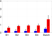
(c) C: $\mu_{2}=11$, $\kappa_{2}=40$

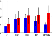
(d) D: $\mu_{2}=11$, $\kappa_{2}=2$

Figure 2: Deviations in detection of infection times

(a) A: $\mu_{2}=100$, $\kappa_{2}=40$

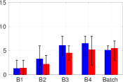
(b) B: $\mu_{2}=100$, $\kappa_{2}=2$

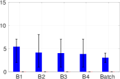
(c) C: $\mu_{2}=11$, $\kappa_{2}=40$

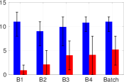
(d) D: $\mu_{2}=11$, $\kappa_{2}=2$

Figure 3: Deviations in detection of parents

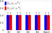
(a) A: $\mu_{2}=100$, $\kappa_{2}=40$

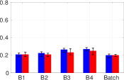
(b) B: $\mu_{2}=100$, $\kappa_{2}=2$

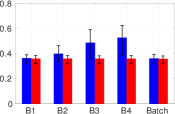
(c) C: $\mu_{2}=11$, $\kappa_{2}=40$

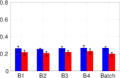
(d) D: $\mu_{2}=11$, $\kappa_{2}=2$

Figure 4: Deviations in detection of link strengths

VI-A Synthetic Data

Since we wish to evaluate the performance of the algorithms in scenarios where the modelling assumptions are exactly met, we generate a dataset based on the model described in Section III. We assume that node $1$ is the source of the infection. For each node $i>1$, we randomly construct $\pi^{i}$ by including each $j\in\{1,\dots,i-1\}$ as a potential parent for $i$ (i.e., $j\in\pi^{i}$) with probability $0.5$. Then, we uniformly choose $j\in\pi^{i}$ for each node $i$ and build a random directed tree ${\mathcal{T}}$ with edges $j\rightarrow i$. We assign the link strength matrix ${\boldsymbol{\alpha}}^{R}=[\alpha^{R}_{ij}]_{N\times N}$ to this model and call them the true link strengths. $\alpha^{R}_{ij}\neq 0$ if and only if $j\in\pi^{i}$. In this case, $\alpha^{R}_{ij}$ is drawn from a gamma distribution $\Gamma(\kappa_{1},\theta_{1})$ if $j\rightarrow i\in{\mathcal{T}}$ and from $\Gamma(\kappa_{2},\theta_{2})$ if $j\rightarrow i\notin{\mathcal{T}}$. We choose the parent of node $i$ from all the nodes $j\in\pi^{i}$ based on a random sampling with weights $\alpha^{R}_{ij}$. These parents are called true parents and are denoted by ${\mathbf{z}}^{R}=[z_{1}^{R},\dots,z_{N}^{R}]^{T}$. Knowing the values of $z^{i}$ and $\alpha^{iz^{i}}$, we then generate the true infection times ${\mathbf{t}}^{R}=[t_{1}^{R},\dots,t_{N}^{R}]^{T}$ based on the geometric distributions described in (3). After choosing the random set of true diffusion parameters $({\mathbf{z}}^{R},{\mathbf{t}}^{R},{\boldsymbol{\alpha}}^{R})$, we choose the length of time series $N_{T}$ to be 10 samples more than the maximum infection time (i.e., $N_{T}=10+\max_{i}t_{i}^{R}$). Finally, we generate data signals ${\mathbf{d}}=\{{\mathbf{d}}^{1},\dots,{\mathbf{d}}^{N}\}$ of length $N_{T}$ based on two different Gaussian distributions for before and after being infected. Hyperparameters $\gamma_{1}^{i}=(\mu_{1},\sigma_{1})$ and $\gamma_{2}^{i}=(\mu_{2},\sigma_{2})$ are used for all nodes $i\in{\mathcal{N}}$.

We aim to investigate whether incorporating the infection diffusion model can improve the estimation of infection times compared to univariate changepoint estimation. Hence, we compare two estimates of infection times: the MAP estimate $\hat{{\mathbf{t}}}$ based on the model and inference techniques described in this paper; and an estimate $\hat{{\mathbf{t}}^{\prime}}=[\hat{t^{\prime}}^{1},\dots,\hat{t^{\prime}}^{N}]^{T}$ derived by maximizing the likelihood of infection time for individual time-series, i.e, $\hat{t^{\prime}}^{i}=\arg\max_{t}f(d_{1:t}^{i};\gamma_{1}^{i})f(d_{t+1:N_{T}}^{i};\gamma_{2}^{i})$.

We examine batch and online Bayesian inference algorithms in a network of $N=20$ nodes. For the online setup, data signals are divided into four blocks of equal length (${\mathbf{B}}_{1}$ to ${\mathbf{B}}_{4}$), i.e., $M=\lfloor\frac{N_{T}}{4}\rfloor$. We test inference algorithms in four scenarios. In all of the scenarios, $\mu_{1}=10$, $\sigma_{1}=\sigma_{2}=1$, $\kappa_{1}=1$, $\theta_{1}=\theta_{2}=0.5$, and $r_{b}=0.5$. In the first scenario (Scenario $A$), $\mu_{2}=100$ and $\kappa_{2}=40$. Hence, not only can the infection times be detected with high likelihood, but also the links that demonstrate the parental relationships can be easily distinguished from the rest of the links due to their high average strengths. In Scenario $B$, $\mu_{2}=100$ and $\kappa_{2}=2$. Therefore, the difference between parent and non-parent links are not significant and the underlying network is not easily detected even though infection times are still recognizable with high likelihood. The same trend exists in Scenarios $C$ and $D$ except for the fact that in these two scenarios the means of two Gaussian distributions are close i.e. in Scenario $C$, $\mu_{2}=11$, $\kappa_{2}=40$ and in Scenario $D$, $\mu_{2}=11$, $\kappa_{2}=2$.

Figure 2 shows the mean and $95\%$ confidence intervals of deviations of the two estimates $\hat{{\mathbf{t}}}$ and $\hat{{\mathbf{t}}^{\prime}}$ from the true infection times ${\mathbf{t}}^{R}$ for 100 realizations of true diffusion parameters. The deviation between two infection time vectors (e.g., $D_{t}(\hat{{\mathbf{t}}},{\mathbf{t}}^{R})$) is defined as the average absolute difference between infection times across all nodes. When the true infection time is greater than the time index of the end of a batch $b$ (i.e., $t_{i}^{R}>{\mathbf{B}}_{b}[Mb]$), we set the true infection time to null for that batch. If either the estimated infection time of a node or its true value is null for a batch $b$, we replace the null value with the end of the batch when calculating the deviation metric. For each of the algorithms, $N_{MCMC}=10^{5}$ samples are generated, the first $N_{burn}=10^{3}$ samples are discarded, and every $N_{thin}=10^{\text{th}}$ of the rest of the samples are kept. The $i^{\text{th}}$ component of $\hat{{\mathbf{t}}}$ denotes the most observed infection time for node $i$ among the stored samples while the $i^{\text{th}}$ component of $\hat{{\mathbf{t}}^{\prime}}$ shows the maximum likelihood estimation of infection time of node $i$ while ignoring other nodes and the underlying network. As expected, the infection times are perfectly detected in the first two scenarios even though in Scenario $B$, the link strengths don’t have significant difference between parent and non-parent links. As opposed to Scenarios $A$ and $B$, deviations of detected infection times from their true values are non-zero in Scenario $C$ and they are even larger in Scenario $D$ where neither infection times nor parental relationships are easy to detect. However, we see that for both batch and online inference methods, exploiting the underlying diffusion network in detecting the infection times leads to more accurate results in average.

Next, we wish to investigate how not knowing the infection times affects the performance of detecting the parental relationships and their strengths. In order to do this, we compare our setup in which all the infection parameters are unknown with a setup in which infection times are perfectly known and ${\mathbf{z}}$ and ${\boldsymbol{\alpha}}$ are the only parameters to be detected. The MAP estimates for the case of unknown infection times are denoted by $\hat{{\mathbf{z}}}$ and $\hat{{\boldsymbol{\alpha}}}$. We use the same Gibbs sampling method to perform inference for the case when the infection times are known (except there is no longer a need to sample infection times). The MAP estimates for this latter case are denoted by $\hat{{\mathbf{z}}^{\prime}}$ and $\hat{{\boldsymbol{\alpha}}^{\prime}}$. We calculate the error metric for parent identification, $D_{z}(\hat{{\mathbf{z}}},{\mathbf{z}}^{R})$, as the average number of nodes whose parents are different in $\hat{{\mathbf{z}}}$ and ${\mathbf{z}}^{R}$. Similarly, $D_{\alpha}(\hat{{\boldsymbol{\alpha}}},{\boldsymbol{\alpha}}^{R})$ denotes the deviation between detected and true link strength values and is equal to the average over all links of the absolute difference between estimated and true $\alpha_{ij}$.

Figures 3 and 4 show the error metrics for the estimation of parents and link strengths for the batch and online algorithms. In Scenarios $A$ and $B$, when infection times are easy to infer, the knowledge of infection times provides little benefits and the error metrics are approximately the same. However, when the infection times are hard to detect (Scenarios $C$ and $D$), the deterioration in the estimation accuracy is more observable. Figure 5 shows the average percentage of samples identifying the correct parents in Scenarios C and D.

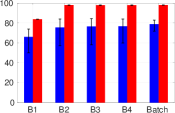
(a) C: $\mu_{2}=11$, $\kappa_{2}=40$

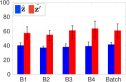
(b) D: $\mu_{2}=11$, $\kappa_{2}=2$

Figure 5: Average percentage of samples identifying the correct parents in Scenarios C and D

VI-B Measles and Chickenpox Data

We study the number of weekly reported cases of measles and chickenpox in England and Wales as shown in Figure 1. The analysis is based on the data from seven large cities (London, Bristol, Liverpool, Manchester, Newcastle, Birmingham, and Sheffield), with populations ranging from $300,000$ to $10$ million (out of a total population of approximately $50$ million). The primary infections occur every two years in the period from September to December of the following year. We focus our analysis on these time windows.

Our model for this data assumes that an infection commences in one city and then by movement of individuals between two cities emerges in one of the other cities. The model does allow for the possibility of infections arising spontaneously due to unrelated influences in multiple cities. In such a case, multiple nodes (cities) have no parent in the inferred model. This can capture scenarios in which infections are caused by interactions with other cities not included in the model (e.g., visitors from other countries). It can also explain the case when the residual infection in a city gives rise to a new outbreak, with no disease transfer from another city.

Quantitative studies (e.g. [24]) have explained the decrease in the number of reported cases in the data after widespread use of a vaccine began in $1968$. Also, studies such as [25] have justified the biennial data peaks, claiming that they were caused by exhaustion and subsequent build-up of susceptibles in the population as well as seasonal changes in virus transmission. Finally, [26] shows that once an infection starts in a region, the number of hospitalized cases can be approximated by a log-normal function of the number of days that have passed since the infection began. The number of hospitalized cases in region $i$ at the $n^{\text{th}}$ week is denoted by $h_{n}^{i}$ and defined as the cumulative number of cases minus the cumulative number of deaths and recoveries. Hence, for $n\geq t^{i}_{1}$ we have

$$h_{n}^{i}=\frac{A_{h}^{i}}{\sqrt{2\pi}\sigma_{h}^{i}7(n-t_{1}^{i})}\exp(-\frac{(\ln[7(n-t_{1}^{i})]-\mu_{h}^{i})^{2}}{2{\sigma_{h}^{i}}^{2}}).$$ (29)

Here $A_{h}^{i}$ is a constant, $\sigma_{h}$ is the variance parameter of the log-normal, and we set $\mu_{h}^{i}=\ln D_{h}^{i}+{\sigma_{h}^{i}}^{2}$, where $D_{h}^{i}=\arg\max_{n}h_{n}^{i}$. The coefficient $7$ is due to the fact that the data is reported weekly.

For each time-series, we use the log-normal function to model the data after an infection. For a candidate infection time, we find $\sigma_{h}^{i}$ and $D_{h}^{i}$ such that the Mean Square Error (MSE) is minimized. We also choose $A_{h}^{i}$ such that $d^{i}_{D_{h}^{i}}=h^{i}_{D_{h}^{i}}$. The “individual infection time estimate” is then the candidate infection time that has minimum MSE after the log-normal fit. We model the residual using a Gaussian distribution. We also assume that the data follows a normal distribution before the individual infection times, i.e.,

$$d_{n}^{i}|t_{1}^{i}\sim\begin{cases}{\mathcal{N}}(\mu_{1}^{i},\sigma_{1}^{i})\quad&\text{if }n>t_{1}^{i},\\ {\mathcal{N}}(h_{n}^{i}+\mu_{2}^{i},\sigma_{2}^{i})\quad&\text{if }n\leq t_{1}^{i}.\end{cases}$$ (30)

In these models, we use empirical variances derived from the previous time-period.

Figure 6 shows an example for 1958-1959 in Liverpool. The candidate infection times are shown by red points in Figure 6a. In 6a, the log-normal fits for each candidate infection time are shown in black. For the example of 6a, the individual infection time estimate is November $1^{\text{st}}$. The quantile-quantile plots in Figures 6b and 6c provide support for the Gaussian model. Results for other years are provided in [27].

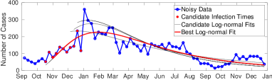
(a) Reported cases for Liverpool in Sep 1958 to Dec 1959

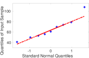
(b) Reported data before the individual infection time

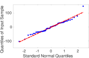
(c) Residual noise after the individual infection time

Figure 6: (a) Reported cases time series with best fit log-normals for different candidate infection times, (b) Quantile-quantile (qq) plot of the reported data before the individual infection time versus standard normal distribution, (c) qq plot of the residual noise after the individual infection time versus standard normal distribution

VI-B1 Estimating Infection Times

Figure 7 shows the reported data for the 1958-1959 study period. The individual infection time estimates are indicated by the change of color from green to red. In all the four successive biennial study periods from 1956 to 1963, Liverpool (node $3$) has the earliest individual infection time estimate. We consider this node as the source of the infection. Given the entire data for each study period, we intend to infer the underlying network as well as the infection times. We use the prior distributions proposed in (3), (4), and (5). The data is modelled as in (30), with $h_{n}^{i}$ calculated for each candidate infection time by minimizing the MSE as explained above. In each study period, we choose the hyper-parameters $\mu_{1}^{i},\sigma_{1}^{i},\mu_{2}^{i},\sigma_{2}^{i},\kappa,\theta$ based on the reported data and the individual infection time estimates for the preceding period.

Any node $j$ whose individual infection time estimate is earlier than the individual infection time estimate of node $i$ in a study period is considered to be a potential parent, i.e. $j\in\pi^{i}$, for the next study period. We generate $N_{MCMC}=10^{5}$ samples, discard the first $N_{burn}=10^{3}$, and store one out of every $N_{thin}=10$ of the rest. The means of the retained samples are used to calculate estimated infection times. These estimated infection times are shown by the black vertical lines in Figure 7. The estimated infection times are quite close to the individual estimates.

VI-B2 Predicting Infection Times

In addition to estimating the infection times, we are interested in predicting them beforehand without having access to the reported data. After we have learned a model, we can form a prediction using only the (individual) infection time estimate of the source node. This allows us to detect the onset of the infection in Liverpool and use it to predict when infections will arise in London and Manchester, for example. We use the inferred network structure for each study period to predict the infection times of the next period. For example, the infection times for 1958-1960 are predicted using the model learned by processing 1956-1958 data. For every stored sample from the distribution, we predict the infection time of node $i$ by $t_{1}^{z_{1}^{i}}+\delta^{iz_{1}^{i}}$ where $\delta^{iz_{1}^{i}}$ is the mean of a geometric distribution with parameter $1-e^{-\alpha_{1}^{iz_{1}^{i}}}$. The mean and $25-75\%$ confidence intervals of these predicted values are respectively shown by the vertical and horizontal blue lines in Figure 7. Figure 8 shows the absolute difference between the average estimated (predicted) infection times with the individual infection time estimates for all nodes except for the source.

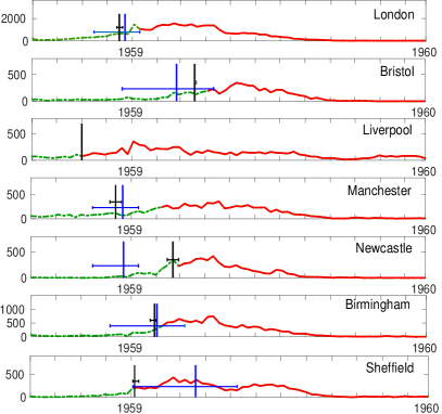
Figure 7: Number of reported cases with estimated and predicted infection times in 1958- 1959. dashed green line: susceptible state, solid red line: infected state (after individual infection time), black lines: mean and 25-75% of estimated values, blue lines: mean and 25-75% of predicted values

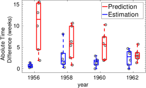
Figure 8: The absolute difference between estimated (predicted) infection times and the individual ones. The central mark of each box is the median, the edge of the box are the 25th and 75th percentiles, the whiskers extend to the highest values not considered as outliers.

VI-C Earthquake Data

In addition to estimating the infection times, our proposed inference approach can be used to detect the underlying network structure. As an example, we use our proposed diffusion framework to study seismic events in different regions of New Zealand. Seismic waves are energy waves generated by earthquakes, volcanic eruptions, and other sources of earth vibration. They travel along layers of the earth and across the surface. Each wave is generated in one location and propagates out to other regions. The epicenter of a seismic event is the location on the surface of the earth directly above the cause of the wave. Our goal is to locate the epicenter of a seismic event and compare it with the reported real location. A seismograph is a device that records earthquake waves and we consider the measuring stations equipped with seismographs as the nodes of the diffusion network. We approximate the seismic event as a propagation of energy waves between these discrete nodes. A seismogram, the graph drawn by a seismograph, is a record of the ground motion as a function of time. The recorded seismograms are used as the observed data signals in our diffusion model. Three examples are shown in Figure 9 for an earthquake that occurred on November 1st 2015.

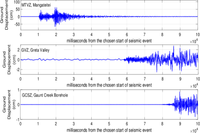
Figure 9: Three recorded seismic waveforms for an earthquake happened on November 1st 2015 (Event ID: 2015p822263)

We choose the prior distribution for link strength values by fitting a Gamma distribution to inverse values of the geographic distance between station pairs. We also assume that seismic waves follow two different Gaussian distributions before and after being infected. This ignores the oscillatory structure and correlations in the time series, but is sufficient for the estimation of the arrival of the seismic wave. We denote the individual changepoint estimate of waveform $i$ by $\hat{t^{\prime}}^{i}$. Denoting the velocity of the seismic waves in the related depth of the earth by $v$, we define the set of potential parents for node $i$ as $\pi_{i}=\{j\in{\mathcal{N}}|\hat{t^{\prime}}^{j}+\frac{D_{ij}}{v}<\hat{t^{\prime}}^{i}\}$ where $D_{ij}$ is the distance between stations $i$ and $j$. More precisely, node $i$ can only be infected by node $j$ if the time difference between their individual changepoints is larger than the time required for the seismic wave to traverse their spatial distance. The precise speed with which seismic waves travel throughout the earth depends on several factors such as composition of the rock, temperature, and pressure. They typically travel at speeds between $1$ and $14$ $\frac{Km}{s}$. In our analysis, we set $v$ to $13\frac{Km}{s}$.

Since we do not know where the source of the infection is, we assume that there is a dummy node within a radius of $D_{i0}$ of each real node. These dummy nodes are candidate sources of the infection and each is a potential parent of its corresponding node. All dummy nodes become infected at the same time, $\underset{i}{\min}(\hat{t^{\prime}}^{i}-\frac{D_{i0}}{v})$. As for the prior distribution of the infection time of node $i$, we know that it is zero for values less than $\frac{D_{iz_{1}^{i}}}{v}$. This probability increases for greater times up to a certain point and then it monotonically increases. We approximate this behaviour with a geometric distribution as in (3).

We run the batch inference algorithm on the diffusion network with $N_{MCMC}=10^{5}$, $N_{burn}=10^{3}$, and $N_{thin}=10$. For each node, we choose the node that marginally maximizes the posterior distribution as its detected parent. This marginal MAP approximation is the parent that occurs most often in the stored samples. We consider the geographical midpoint of the nodes that are infected by their dummy nodes as the approximate location of the epicenter. The detected and real epicenters of two seismic events are shown in Figure 10 where $v=13\frac{Km}{s}$ and $D_{i0}=10Km$ is used. We see that a tree-like network structure exists where the root is close to the real epicenter of the seismic event.

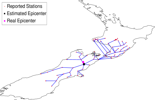
(a) Event ID: 2016p105478

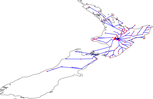
(b) Event ID: 2015p822263

Figure 10: Detected network structure for two seismic events in New Zealand, The distance between real and detected epicenters are (a) $29Km$ and (b) $15Km$

VII Conclusion

This paper presented a Bayesian framework for modeling the diffusion of some sort of a contagion over a graph structure. We formulated the diffusion process by introducing three main sets of parameters: parental relationships, the strength of connections between node pairs, and infection times. The main issue we addressed in this work was to simultaneously infer these three sets of parameters using data signals observed at each of these individual nodes. In order to do so, we applied MCMC techniques to generate samples from the posterior distribution of these parameters. One of the main contributions of this paper is to address applications in which parameters must be estimated before all of the data has been acquired. We addressed this concern by developing an online version of the inference algorithm.

We evaluated the performance of our proposed inference approaches on both synthetic and real world network scenarios. In the synthetic dataset, model assumptions are exactly met and the ground truth is perfectly known. Simulation results showed that considering the underlying network structure in estimating infection times improves accuracy compared to processing the data at each node individually. We compared the precision of detecting the network structure (parental relationships and link strengths) in scenarios with known and unknown infection times. Finally, we tested our proposed inference algorithm in practical scenarios. First, we showed how the algorithm can use the number of reported cases of a contagious disease as the observed time series to construct estimates and predictions of the time of the year when disease outbreaks occur in a particular region. We then used the inference approach to locate the epicenters of earthquakes using the seismic waveforms recorded at seismic stations.

In future work, we aim to extend our methodology, developing more sophisticated algorithms that account for more complicated infection models, e.g., the SEIR (Susceptible-Exposed-Infected-Recovered) model for observed time series. We also intend to improve our online inference method so that it can process scenarios with dynamic networks where nodes enter or leave the network or the set of potential parents changes over time.

Appendix A Proof of Proposition 1

.

Replacing (21)-(25) in (26), we can check that the integrals are separable for different nodes. Hence, (26) is equal to

$$\prod_{i\in{\mathcal{N}}}\sum_{t_{b}^{i}\in{\mathcal{S}}_{1}}h_{t}(t_{b}^{i}|{\mathbf{x}}_{b-1};{t_{b}^{ML}}^{i})\times\prod_{k\in\pi^{i}}h_{\alpha z}^{k}(t_{b}^{i})\,,$$ (31)

where

$$h_{\alpha z}^{k}(t_{b}^{i})=\int_{0}^{\infty}h_{\alpha}(\alpha_{b}^{ki}|t_{b}^{i},{\mathbf{x}}_{b-1})\sum_{z_{b}^{i}\in{\mathcal{S}}_{2}}h_{z}(z_{b}^{i}|t_{b}^{i},{\boldsymbol{\alpha}}_{b},{\mathbf{x}}_{b-1})d_{\alpha_{b}^{ki}}\,.$$ (32)

For each node $i$, we calculate the component in (31) for two cases of $t_{b-1}^{i}=\phi$ and $t_{b-1}^{i}\neq\phi$ separately. When $t_{b-1}^{i}\neq\phi$, the integral is equal to

$$\sum_{t_{b}^{i}\in{\mathcal{S}}_{1}} \delta(t_{b}^{i}-t_{b-1}^{i})\times$$ (33)

$$\prod_{k\in\pi^{i}}\int_{0}^{\infty}\sum_{z_{b}^{i}\in{\mathcal{S}}_{2}}\delta(\alpha_{b}^{ik}-\alpha_{b-1}^{ik})\delta(z_{b}^{i}-z_{b-1}^{i})d_{\alpha_{b}^{ik}}=1\,.$$

When $t_{b-1}^{i}=\phi$, we start from the innermost integral of (32)

$$\sum_{z_{b}^{i}\in{\mathcal{S}}_{2}} h_{z}(z_{b}^{i}|t_{b}^{i},{\boldsymbol{\alpha}}_{b},t_{b-1}^{i})$$

$$=\begin{cases}1&t_{b}^{i}=\phi\,,\\ 1-\frac{\sum_{l\in\pi_{b}^{i}}\alpha_{b}^{il}}{\sum_{j\in\pi^{i}}\alpha_{b}^{ij}}+\frac{\sum_{l\in\pi_{b}^{i}}\alpha_{b}^{il}}{\sum_{j\in\pi^{i}}\alpha_{b}^{ij}}&t_{b}^{i}\neq\phi\,.\end{cases}$$ (34)

Hence, $h_{\alpha z}^{k}(t_{b}^{i})=\int_{0}^{\infty}\Gamma(\kappa_{ki},\theta_{ki})d_{\alpha_{b}^{ki}}=1$. Similarly for $t_{b-1}^{i}=\phi$, $\sum_{t_{b}^{i}\in{\mathcal{S}}_{1}}h_{t}(t_{b}^{i})=1$. Therefore (31) always equals $1$ and $h({\mathbf{x}}_{b}|{\mathbf{x}}_{b-1};{\mathbf{t}}_{b}^{ML})$ is a probability distribution function. ∎

Appendix B Refinement Full Conditional Distributions

The full conditional distributions for GS in the refinement step can be derived as follows.
a) For parent of node $i\in{\mathcal{N}}$

$$f(z_{b}^{i}|{\mathbf{x}}_{b-1}^{m},{\mathbf{d}}_{{\mathbf{B}}_{b}},{\mathbf{z}}_{b}^{\overline{i}},{\mathbf{t}}_{b},{\boldsymbol{\alpha}}_{b})\propto$$ (35)

$$\begin{cases}\delta(z_{b}^{i}-\phi)&\text{if }{t^{i}}_{b-1}^{m}=\phi,t_{b}^{i}=\phi\,,\\ \delta(z_{b}^{i}-{z^{i}}_{b-1}^{m})&\text{if }{t^{i}}_{b-1}^{m}\neq\phi,t_{b}^{i}\neq\phi\,,\\ f(t_{b}^{i}|z_{b}^{i},\alpha_{b}^{iz_{b}^{i}},t_{b}^{z_{b}^{i}})f(z_{b}^{i}|\alpha_{b}^{ik})_{k\in\pi^{i}}&\text{if }{t^{i}}_{b-1}^{m}=\phi,t_{b}^{i}\neq\phi\,.\\ \end{cases}$$

b) For infection time of node $i\in{\mathcal{N}}$

$$f(t_{b}^{i}|{\mathbf{x}}_{b-1}^{m},{\mathbf{d}}_{{\mathbf{B}}_{b}},{\mathbf{z}}_{b},{\mathbf{t}}_{b}^{\overline{i}},{\boldsymbol{\alpha}}_{b})\propto$$ (36)

$$\begin{cases}\delta(t_{b}^{i}-{t^{i}}_{b-1}^{m})&\text{if }{t^{i}}_{b-1}^{m}\neq\phi\,,\\ \begin{tabular}[]{@{}c@{}}$f({\mathbf{d}}_{{\mathbf{B}}_{b}}^{i}|t_{b}^{i})f(t_{b}^{i}|z_{b}^{i},\alpha_{b}^{iz_{b}^{i}},t_{b}^{z_{b}^{i}})\times$\\ $\prod_{k\in{\mathcal{C}}_{b}^{i}}f(t_{b}^{k}|\alpha_{b}^{ki},t_{b}^{i})$\end{tabular}&\text{if }{t^{i}}_{b-1}^{m}=\phi\,.\\ \end{cases}$$

c) For link strength between nodes $i\in{\mathcal{N}}$ and $j\in\pi^{i}$

$$f(\alpha_{b}^{ij}|{\mathbf{x}}_{b-1}^{m},{\mathbf{d}}_{{\mathbf{B}}_{b}},{\mathbf{z}}_{b},{\mathbf{t}}_{b},{\boldsymbol{\alpha}}_{b}^{\overline{ij}})\propto$$ (37)

$$\begin{cases}f(\alpha_{b}^{ij})&\text{if }{t^{i}}_{b-1}^{m}=\phi,t_{b}^{i}=\phi\,,\\ \delta(\alpha_{b}^{ij}-{\alpha^{ij}}_{b-1}^{m})&\text{if }{t^{i}}_{b-1}^{m}\neq\phi,t_{b}^{i}\neq\phi\,,\\ f(t_{b}^{i}|z_{b}^{i},\alpha_{b}^{iz_{b}^{i}},t_{b}^{z_{b}^{i}})f(z_{b}^{i}|{\boldsymbol{\alpha}}_{b})f(\alpha_{b}^{ij})&\text{if }{t^{i}}_{b-1}^{m}=\phi,t_{b}^{i}\neq\phi\,.\end{cases}$$

Here ${t^{i}}_{b-1}^{m}$, ${z^{i}}_{b-1}^{m}$, and ${\alpha^{ij}}_{b-1}^{m}$ respectively denote the infection time of node $i$, the parent of node $i$, and the link strength between nodes $i$ and $j$ in the sample ${\mathbf{x}}_{b-1}^{m}$.

References

- [1] A. Guille, H. Hacid, C. Favre, and D. A. Zighed, “Information diffusion in online social networks: A survey,” ACM SIGMOD Record, vol. 42, no. 2, pp. 17–28, 2013.
- [2] J. Yang and J. Leskovec, “Modeling information diffusion in implicit networks,” in Proc. IEEE Int. Conf. Data Min. (ICDM), 2010, pp. 599–608.
- [3] Y. Wang, G. Xiang, and S.-K. Chang, “Sparse linear influence model for hot user selection on mining a social network,” in Proc. Int. Conf. Soft. Eng. and Knowl. Eng. (SEKE), 2012, pp. 1–6.
- [4] M. Gomez-Rodriguez, D. Balduzzi, and B. Schölkopf, “Uncovering the temporal dynamics of diffusion networks,” in Proc. Int. Conf. Mach. Learn. (ICML), 2011, pp. 561–568.
- [5] M. Gomez-Rodriguez, J. Leskovec, and A. Krause, “Inferring networks of diffusion and influence,” ACM Trans. Knowl. Discov. from Data, vol. 5, no. 4, p. 21, 2012.
- [6] H. N. Ozsoylev, J. Walden, M. D. Yavuz, and R. Bildik, “Investor networks in the stock market,” Rev. Financ. Stud., vol. 27, no. 5, pp. 1323–1366, 2014.
- [7] K. R. Ahern, “Network centrality and the cross section of stock returns,” Available at SSRN 2197370, 2013.
- [8] E. Sefer and C. Kingsford, “Convex risk minimization to infer networks from probabilistic diffusion data at multiple scales,” in Proc. Int. Conf. Data Eng. (ICDE), 2015, pp. 663–674.
- [9] D. A. Shamma, L. Kennedy, and E. F. Churchill, “Peaks and persistence: modeling the shape of microblog conversations,” in Proc. ACM Conf. Comput. Supported Cooperative Work and Social Comput. (CSCW), 2011, pp. 355–358.
- [10] M. Gomez-Rodriguez, J. Leskovec, and B. Schölkopf, “Structure and dynamics of information pathways in online media,” in Proc. ACM Int. Conf. Web Search and Data Min. (WSDM), 2013, pp. 23–32.
- [11] M. Farajtabar, Y. Wang, M. Gomez-Rodriguez, S. Li, H. Zha, and L. Song, “Coevolve: A joint point process model for information diffusion and network co-evolution,” in Proc. Advances in Neural Info. Process. Syst. (NIPS), 2015, pp. 1945–1953.
- [12] V. R. Embar, R. K. Pasumarthi, and I. Bhattacharya, “A bayesian framework for estimating properties of network diffusions,” in Proc. ACM SIGKDD Int. Conf. Knowl. Discov. and Data Min. (KDD), 2014, pp. 1216–1225.
- [13] M. Farajtabar, M. Gomez-Rodriguez, N. Du, M. Zamani, H. Zha, and L. Song, “Back to the past: Source identification in diffusion networks from partially observed cascades,” in Proc. Int. Conf. Artif. Intell. and Stat., 2015, pp. 232–240.
- [14] K. Amin, H. Heidari, and M. Kearns, “Learning from contagion (without timestamps),” in Proc. Int. Conf. Mach. Learn. (ICML), 2014, pp. 1845–1853.
- [15] A. Y. Lokhov and T. Misiakiewicz, “Efficient reconstruction of transmission probabilities in a spreading process from partial observations,” arXiv preprint arXiv:1509.06893, 2015.
- [16] S. Shaghaghian and M. Coates, “Bayesian inference of diffusion networks with unknown infection times,” in Proc. IEEE Int. Workshop Stat. Signal Process. (SSP), 2016, pp. 1–5.
- [17] I. A. Eckley, P. Fearnhead, and R. Killick, “Analysis of changepoint models,” Bayesian Time Series Model., pp. 205–224, 2011.
- [18] P. Fearnhead, “Exact Bayesian curve fitting and signal segmentation,” IEEE Trans. Signal Process., vol. 53, no. 6, pp. 2160–2166, 2005.
- [19] R. Killick, P. Fearnhead, and I. Eckley, “Optimal detection of changepoints with a linear computational cost,” J. American Stat. Assoc., vol. 107, no. 500, pp. 1590–1598, 2012.
- [20] D. S. Matteson and N. A. James, “A nonparametric approach for multiple change point analysis of multivariate data,” J. American Stat. Assoc., vol. 109, no. 505, pp. 334–345, 2014.
- [21] X. Xuan and K. Murphy, “Modeling changing dependency structure in multivariate time series,” in Proc. Int. Conf. Mach. learn., 2007, pp. 1055–1062.
- [22] F. Septier, S. K. Pang, A. Carmi, and S. Godsill, “On MCMC-based particle methods for Bayesian filtering: Application to multitarget tracking,” in Proc. IEEE Int. Workshop Comput. Advances in Multi-Sensor Adaptive Process. (CAMSAP), 2009, pp. 360–363.
- [23] W. K. Hastings, “Monte carlo sampling methods using markov chains and their applications,” Biometrika, vol. 57, no. 1, pp. 97–109, 1970.
- [24] B. Bolker and B. Grenfell, “Impact of vaccination on the spatial correlation and persistence of measles dynamics,” Proc. Nat. Academy Sci., vol. 93, no. 22, pp. 12 648–12 653, 1996.
- [25] B. Bolker, “Chaos and complexity in measles models: a comparative numerical study,” Math. Med. and Biol., vol. 10, no. 2, pp. 83–95, 1993.
- [26] W. Wang, Z. Wu, C. Wang, and R. Hu, “Modelling the spreading rate of controlled communicable epidemics through an entropy-based thermodynamic model,” Science China Phys., Mech., and Astro., vol. 56, no. 11, pp. 2143–2150, 2013.
- [27] S. Shaghaghian and M. Coates, “Online Bayesian inference of diffusion networks,” Dept. Elect. and Comput. Eng., McGill Univ., Montreal, QC, Tech. Rep., 2016.