Effects of $Z_{b}$ states and bottom meson loops on
$\Upsilon(4S)\to\Upsilon(1S,2S)\pi^{+}\pi^{-}$ transitions

Abstract

We study the dipion transitions $\Upsilon(4S)\rightarrow\Upsilon(nS)\pi^{+}\pi^{-}$ $(n=1,2)$. In particular, we consider the effects of the two intermediate bottomoniumlike exotic states $Z_{b}(10610)$ and $Z_{b}(10650)$ as well as bottom meson loops. The strong pion–pion final-state interactions, especially including channel coupling to $K\bar{K}$ in the $S$-wave, are taken into account model-independently by using dispersion theory. Based on a nonrelativistic effective field theory we find that the contribution from the bottom meson loops is comparable to those from the chiral contact terms and the $Z_{b}$-exchange terms. For the $\Upsilon(4S)\rightarrow\Upsilon(2S)\pi^{+}\pi^{-}$ decay, the result shows that including the effects of the $Z_{b}$-exchange and the bottom meson loops can naturally reproduce the two-hump behavior of the $\pi\pi$ mass spectra. Future angular distribution data are decisive for the identification of different production mechanisms. For the $\Upsilon(4S)\rightarrow\Upsilon(1S)\pi^{+}\pi^{-}$ decay, we show that there is a narrow dip around $1\,\text{GeV}$ in the $\pi\pi$ invariant mass distribution, caused by the final-state interactions. The distribution is clearly different from that in similar transitions from lower $\Upsilon$ states, and needs to be verified by future data with high statistics. Also we predict the decay width and the dikaon mass distribution of the $\Upsilon(4S)\rightarrow\Upsilon(1S)K^{+}K^{-}$ process.

I Introduction

The processes of dipion emission of the bottomonia $\Upsilon(mS)\to\Upsilon(nS)\pi\pi$ are important for understanding the heavy-quarkonium dynamics and low-energy QCD. Because the bottomonia are expected to be nonrelativistic and compact, the method of the QCD multipole expansion Voloshin1980 ; Novikov1981 ; Kuang1981 ; Kuang2006 is often used to study these transitions, where the pions emitted come from the hadronization of soft gluons. Though successful in describing many $\Upsilon(mS)\to\Upsilon(nS)\pi\pi$ processes, a well-known anomaly about the method of the QCD multipole expansion is that it cannot reproduce the two-hump behavior in the experimental $\pi\pi$ invariant mass spectra of the decays $\Upsilon(3S)\rightarrow\Upsilon(1S)\pi\pi$ and $\Upsilon(4S)\rightarrow\Upsilon(2S)\pi^{+}\pi^{-}$ Eichten2008 ; Guo2005 ; Guo2007:4S . In a previous study Chen2016 , we found that by including the effects of the two bottomoniumlike exotic states $Z_{b}(10610)$ and $Z_{b}(10650)$ discovered by the Belle Collaboration Belle2011:1 ; Belle2012:1 as well as the $\pi\pi$ final-state interaction (FSI), the anomaly of the $\Upsilon(3S)\rightarrow\Upsilon(1S)\pi\pi$ process can be naturally explained. Such an analysis is a modern version of the much earlier studies in Refs. Voloshin:1982ij ; Anisovich:1995zu , where an isovector $b\bar{b}q\bar{q}$ state was considered. Although the direct decay of $Z_{b}$ into $\Upsilon(4S)\pi$ is kinematically impossible, it may be illuminating to analyze the effect of the $Z_{b}$-exchange mechanism in the $\Upsilon(4S)\rightarrow\Upsilon(1S,2S)\pi^{+}\pi^{-}$ processes, which is performed in this study. In this context it is important to note that improved data on $\Upsilon(nS)$ decays are to be expected from Belle-II that will start operation soon—for a detailed discussion of prospects for various decays relevant for this study we refer to Ref. Bondar:2016hva .

The $\Upsilon(4S)$ meson is above the $B\bar{B}$ threshold and decays predominantly to $B\bar{B}$, so loop effects with intermediate bottom mesons may play an important role in $\Upsilon(4S)\to\Upsilon(nS)\pi\pi$ $(n=1,2)$. Also, the inclusion of the loops will introduce non-analyticities arising from the $B\bar{B}$ threshold needed to be taken into account in dispersion theory, which will be discussed later. Because the bottomonia are close to the open-bottom meson production threshold, the velocity of the intermediate bottom mesons is small and can be treated as an expansion parameter to build power-counting rules in a nonrelativistic effective field theory (NREFT) Guo2009:PRL ; Guo2011:effect ; Martin2013 . Within the NREFT scheme, we will calculate the dominant box diagrams in the dipion emissions of $\Upsilon(4S)$, and find that their contribution is comparable in size to the chiral contact terms and the $Z_{b}$-exchange graphs.

In the $\Upsilon(4S)\to\Upsilon(1S)\pi\pi$ process, the dipion invariant mass reaches above the $K\bar{K}$ threshold, so the coupled-channel FSI in the $S$-wave is strong and needs to be taken into account. Based on analyticity and unitarity, dispersion theory can achieve this in a model-independent way. In this study, we will use dispersion theory in the form of modified Omnès solutions, in which the left-hand-cut contribution is approximated by the sum of the $Z_{b}$-exchange mechanism and the bottom meson loops. At low energies, the amplitude should agree with the leading chiral results, so the subtraction functions can be determined by matching to chiral contact terms. For the leading contact couplings of two $S$-wave bottomonia to an even number of light pseudoscalar mesons, we will adopt the Lagrangian given in Ref. Mannel , constructed in the spirit of the chiral and the heavy-quark nonrelativistic expansions.

This paper is organized as follows. In Sec. II, we present the theoretical framework and elaborate on the calculation of the amplitudes as well as the dispersive treatment of the FSI. In Sec. III, we fit the experimental data of the $\pi\pi$ invariant mass distribution to determine the coupling constants, and discuss the contributions of different mechanisms. A summary will be given in Sec. IV.

II Theoretical framework

II.1 Lagrangians

Because in the heavy-quark limit the spin of the heavy quarks decouples, it is convenient to introduce the heavy quarkonia and heavy hadrons in terms of spin multiplets. One has $J\equiv\mathbf{\Upsilon}\cdot\bm{\sigma}+\eta_{b}$, where $\mathbf{\Upsilon}$ and $\eta_{b}$ annihilate the $\Upsilon$ and $\eta_{b}$ states, respectively, and $\bm{\sigma}$ contains the Pauli matrices Guo2011 . The bottom mesons are collected in $H_{a}=\mathbf{V}_{a}\cdot\bm{\sigma}+P_{a}$ with $P_{a}(V_{a})=(B^{(*)-},\bar{B}^{(*)0},\bar{B}_{s}^{(*)0})$, and $\bar{H}_{a}=-\bar{\mathbf{V}}_{a}\cdot\bm{\sigma}+\bar{P}_{a}$ with $\bar{P}_{a}(\bar{V}_{a})=(B^{(*)+},B^{(*)0},B_{s}^{(*)0})$ Mehen2008 .

The effective Lagrangian for the contact $\Upsilon\Upsilon^{\prime}\pi\pi$ and $\Upsilon\Upsilon^{\prime}K\bar{K}$ coupling, at the lowest order in the chiral as well as the heavy-quark expansion, reads Mannel ; Chen2016

$$\mathscr{L}_{\Upsilon\Upsilon^{\prime}\Phi\Phi}=\frac{c_{1}}{2}\langle J^{\dagger}J^{\prime}\rangle\langle u_{\mu}u^{\mu}\rangle+\frac{c_{2}}{2}\langle J^{\dagger}J^{\prime}\rangle\langle u_{\mu}u_{\nu}\rangle v^{\mu}v^{\nu}+\mathrm{h.c.}\,,$$ (1)

where $v^{\mu}=(1,\mathbf{0})$ is the velocity of the heavy quark. The Goldstone bosons of the spontaneous breaking of chiral symmetry can be parametrized as

$$u_{\mu} =i\left(u^{\dagger}\partial_{\mu}u\,-\,u\partial_{\mu}u^{\dagger}\right)\,,\qquad u=\exp\Big{(}\frac{i\Phi}{\sqrt{2}F}\Big{)}\,,$$

$$\Phi =\begin{pmatrix}{\frac{1}{\sqrt{2}}\pi^{0}+\frac{1}{\sqrt{6}}\eta_{8}}&{\pi^{+}}&{K^{+}}\\ {\pi^{-}}&{-\frac{1}{\sqrt{2}}\pi^{0}+\frac{1}{\sqrt{6}}\eta_{8}}&{K^{0}}\\ {K^{-}}&{\bar{K}^{0}}&{-\frac{2}{\sqrt{6}}\eta_{8}}\\ \end{pmatrix},$$ (2)

where $F$ is the pseudo-Goldstone boson decay constant, and we will use $F_{\pi}=92.2\,\text{MeV}$ for the pions and $F_{K}=113.0\,\text{MeV}$ for the kaons. The two operators in Eq. (1) both scale as $\mathcal{O}(q_{\pi}^{2})$ in the expansion in (soft) pion momenta $q_{\pi}$.

The leading Lagrangian for the $Z_{b}\Upsilon\pi$ interaction, which is needed in the calculation of the mechanism $\Upsilon(mS)\to Z_{b}\pi\to\Upsilon(nS)\pi\pi$, reads Guo2011

$$\mathscr{L}_{Z_{b}\Upsilon\pi}=\sum_{j=1,2}\sum_{l}C_{Z_{bj}\Upsilon(lS)\pi}\Upsilon^{i}(lS)\langle{Z^{i}_{bj}}^{\dagger}u_{\mu}\rangle v^{\mu}+\mathrm{h.c.}\,,$$ (3)

where $Z_{b1}$ and $Z_{b2}$ are used to refer to $Z_{b}(10610)$ and $Z_{b}(10650)$, respectively. The $Z_{b}$ states are collected in the matrix as

$$Z^{i}_{bj}=\left({\begin{array}[]{*{3}c}\frac{1}{\sqrt{2}}Z^{0i}_{bj}&Z^{+i}_{bj}&0\\ Z^{-i}_{bj}&-\frac{1}{\sqrt{2}}Z^{0i}_{bj}&0\\ 0&0&0\end{array}}\right)\,.$$ (4)

Note that since strange partners of the $Z_{b}$ states, $Z_{bs}$, have not been observed, we set the corresponding matrix entries in Eq. (4) to zero.

To calculate the box diagrams, we need the Lagrangian for the coupling of the $S$-wave bottomonium fields to the bottom and antibottom mesons Guo2009:PRL ,

$$\mathscr{L}_{JHH}=\frac{i\,g_{JHH}}{2}\langle J^{\dagger}H_{a}\bm{\sigma}\cdot\!\overleftrightarrow{\partial}\!\bar{H}_{a}\rangle+{\rm h.c.}\,,$$ (5)

where $A\overleftrightarrow{\partial}\!B\equiv A(\overrightarrow{\partial}B)-(\overrightarrow{\partial}A)B$. We also need the Lagrangian for the axial coupling of the Goldstone bosons to the bottom and antibottom mesons, which at leading order in heavy-flavor chiral perturbation theory is given by Burdman:1992gh ; Wise:1992hn ; Yan:1992gz ; Casalbuoni:1996pg ; Mehen2008

$$\mathscr{L}_{HH\Phi}=\frac{g_{\pi}}{2}\langle\bar{H}_{a}^{\dagger}\bm{\sigma}\cdot\mathbf{u}_{ab}\bar{H}_{b}\rangle-\frac{g_{\pi}}{2}\langle H_{a}^{\dagger}H_{b}\bm{\sigma}\cdot\mathbf{u}_{ba}\rangle,$$ (6)

where $u^{i}=-\sqrt{2}\partial^{i}\Phi/F+\mathcal{O}(\Phi^{3})$ corresponds to the three-vector components of $u_{\mu}$ as defined in Eq. (2). Here we will use $g_{\pi}=0.5$ from a recent lattice QCD calculation Bernardoni:2014kla .

II.2 Power counting of the loops

Since the $\Upsilon(4S)$ is above the $B\bar{B}$ threshold and decays predominantly into $B\bar{B}$ pairs, the loop mechanism with intermediate bottom mesons may play a significant role in the bottomonium transitions $\Upsilon(4S)\rightarrow\Upsilon(nS)\pi^{+}\pi^{-}$. In this section, we will analyze the power counting of different kinds of loops, based on NREFT Guo2009:PRL ; Guo2011:effect ; Martin2013 . In NREFT, the expansion parameter is the typical velocity of the intermediate heavy meson, namely $\nu=\sqrt{|m_{\Upsilon(lS)}-m_{B^{(*)}}-m_{B^{(*)}}|/m_{B^{(*)}}}$, and $\nu\ll 1$ since $\Upsilon(lS)$ are close to the $B^{(*)}\bar{B}^{(*)}$ thresholds. Each nonrelativistic propagator is counted as $1/\nu^{2}$, and the full integral measure $\int d^{4}l$ as $\nu^{5}$. More details of the power counting rules are elaborated in Ref. Guo2011:effect .

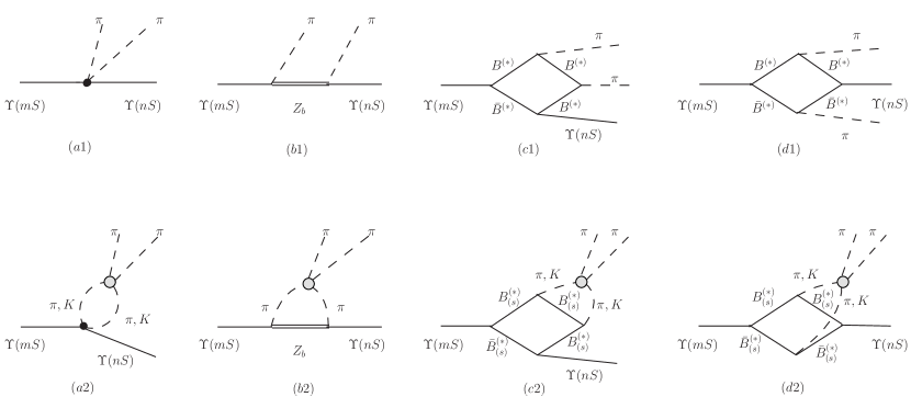
Figure 1: Feynman diagrams considered for the $\Upsilon(mS)\rightarrow\Upsilon(nS)\pi\pi$ processes. The crossed diagrams of (b1), (c1), (b2), and (c2) are not shown explicitly. The gray blob denotes the final-state interaction.

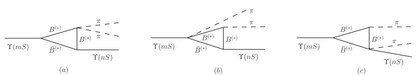
Figure 2: Subleading contributions for $\Upsilon(mS)\rightarrow\Upsilon(nS)\pi\pi$ that are suppressed in comparison to the four-point functions in Fig. 1 and hence not considered in the calculations. The corresponding power counting arguments are given in the main text.

Without considering the FSI, there are five different kinds of loop contributions, namely the box diagrams displayed in Fig. 1 (c1), (d1), and the triangle diagrams displayed in Fig. 2 (a)–(c). We analyze them one by one as follows:

1. Box diagrams, namely Fig. 1 (c1), (d1): As indicated in Eq. (6), the vertex for the axial coupling of the pion to the bottom mesons is proportional to the external momentum of the pion $q_{\pi}$. Both the vertices for the initial and final bottomonia are in a $P$-wave, and the product of the two vertices can be counted as $\mathcal{O}(\nu^{2})$, so the box diagrams are counted as $\nu^{5}\nu^{2}q_{\pi}^{2}/\nu^{8}=q_{\pi}^{2}/\nu.$ Note that these contributions thus have the same scaling in pion momenta as the leading $\Upsilon\Upsilon^{\prime}\pi\pi$ contact terms from the Lagrangian Eq. (1), but are formally enhanced by $1/\nu$ in the non-relativistic velocity parameter.

2. Fig. 2 (a): The leading $B^{(*)}B^{(*)}\pi\pi$ vertex comes from the covariant chiral derivative term $\langle H_{a}^{\dagger}(iD_{0})_{ba}H_{b}\rangle=\langle H_{a}^{\dagger}(i\partial_{0}-iV_{0})_{ba}H_{b}\rangle$ Stewart ; Mehen2006 , in which the pion pair produced by the vector current, $V^{\mu}=\frac{1}{2}(u^{\dagger}\partial^{\mu}u+u\partial^{\mu}u^{\dagger})$, cannot form a positive-parity and $C$-parity state, so this leading vertex does not contribute to the $\Upsilon(mS)\rightarrow\Upsilon(nS)\pi\pi$ processes. Isoscalar, $PC=++$ pion pairs only enter in the next order $\mathcal{O}(q_{\pi}^{2})$ from point vertices. For the vertices of the initial and final bottomonia, both of them are in $P$-waves, so the product of them can be counted as $\mathcal{O}(\nu^{2})$. These diagrams hence count as $\nu^{5}\nu^{2}q_{\pi}^{2}/\nu^{6}=\nu q_{\pi}^{2}$, and are suppressed compared to the contact terms $\propto c_{1,2}$ by the factor $\nu$.

3. Fig. 2 (b), (c): The leading $\Upsilon(lS)B^{(*)}\bar{B}^{(*)}\pi$ vertex given by $\langle J\bar{H}_{a}^{\dagger}H_{b}^{\dagger}\rangle u_{ab}^{0}$ Mehen2013 is proportional to the energy of the pion, $E_{\pi}\sim q_{\pi}$. In Fig. 2 (b), the vertex for the initial bottomonium is in an $S$-wave, and the vertex for the final bottomonium is in a $P$-wave, so the loop momentum must contract with the external momentum $q_{\pi}$ and hence the $P$-wave vertex scales as $\mathcal{O}(q_{\pi})$. For this reason, Fig. 2 (b) is counted as $\nu^{5}q_{\pi}^{3}/(\nu^{6}m_{B})=q_{\pi}^{3}/(\nu m_{B})$, where the factor $m_{B}$ has been introduced to match the dimension with the scaling for cases 1 and 2. Analogous arguments hold for Fig. 2 (c). This class of diagrams is therefore suppressed in the chiral expansion in pion momenta, compared to the $c_{1,2}$ terms.

We find thus that according to the power counting the box diagrams are dominant among the loop contributions, and the only ones not expected to be suppressed relative to the tree-level contact terms. We will therefore only calculate these in the present study. Note that all (box and triangle) loop contributions discussed here are ultraviolet-finite, and do not require the additional introduction of counterterms.

II.3 Tree-level amplitudes and box diagram calculation

First we define the Mandelstam variables in the decay process of $\Upsilon(mS)(p_{a})\to\Upsilon(nS)(p_{b})P(p_{c})P(p_{d})$

$$s =(p_{c}+p_{d})^{2},\qquad t_{P}=(p_{a}-p_{c})^{2}\,,\qquad u_{P}=(p_{a}-p_{d})^{2}\,,$$

$$3s_{0P} \equiv s+t_{P}+u_{P}=m_{\Upsilon(mS)}^{2}+m_{\Upsilon(nS)}^{2}+2m_{P}^{2}\,,$$ (7)

where $P$ denotes the pseudoscalar $\pi$ or $K$, since we also need to take into account the virtual process $\Upsilon(mS)(p_{a})\to\Upsilon(nS)(p_{b})K(p_{c})\bar{K}(p_{d})$ in the coupled-channel FSI. $t_{P}$ and $u_{P}$ can be expressed in terms of $s$ and the helicity angle $\theta$ according to

$$t_{P} =\frac{1}{2}\left[3s_{0P}-s+\kappa_{P}(s)\cos\theta\right]\,, u_{P} =\frac{1}{2}\left[3s_{0P}-s-\kappa_{P}(s)\cos\theta\right]\,,$$

$$\kappa_{P}(s) \equiv\sigma_{P}\lambda^{1/2}\big{(}m_{\Upsilon(mS)}^{2},m_{\Upsilon(nS)}^{2},s\big{)}\,, \sigma_{P} \equiv\sqrt{1-\frac{4m_{P}^{2}}{s}}\,,$$ (8)

where $\theta$ is defined as the angle between the initial $\Upsilon(mS)$ and the positive pseudoscalar in the rest frame of the $PP$ system, and $\lambda(a,b,c)=a^{2}+b^{2}+c^{2}-2(ab+ac+bc)$. We define $\mathbf{q}$ as the 3-momentum of the final bottomonium in the rest frame of the initial state with

$$|\mathbf{q}|=\frac{1}{2m_{\Upsilon(mS)}}\lambda^{1/2}\big{(}m_{\Upsilon(mS)}^{2},m_{\Upsilon(nS)}^{2},s\big{)}\,.$$ (9)

The calculation of the tree amplitudes is very similar to our previous study of $\Upsilon(3S)$ decays Chen2016 , so here we just quote the partial-wave-projected results. Parity and $C$-parity conservation require the pion pair to have even relative angular momentum $l$. We will only consider the $S$-wave and $D$-wave components in this study, neglecting the effects of higher partial waves. For the $S$-wave, the amplitudes of the chiral contact term and the $Z_{b}$-exchange term read

$$M_{0}^{\chi,P}(s) =-\frac{2}{F_{P}^{2}}\sqrt{m_{\Upsilon(mS)}m_{\Upsilon(nS)}}\bigg{\{}c_{1}\left(s-2m_{P}^{2}\right)+\frac{c_{2}}{2}\bigg{[}s+\mathbf{q}^{2}\Big{(}1-\frac{\sigma_{P}^{2}}{3}\Big{)}\bigg{]}\bigg{\}}\,,$$ (10)

$$\hat{M}_{0}^{Zb,\pi}(s) =-\frac{2\sqrt{m_{\Upsilon(mS)}m_{\Upsilon(nS)}}}{F_{\pi}^{2}\kappa_{\pi}(s)}\sum_{i=1,2}m_{Z_{bi}}C_{mn,i}\Big{\{}\big{(}s+|\mathbf{q}|^{2}\big{)}Q_{0}(y_{\pi i})-|\mathbf{q}|^{2}\sigma_{\pi}^{2}\big{[}y_{\pi i}^{2}Q_{0}(y_{\pi i})-y_{\pi i}\big{]}\Big{\}}\,,$$ (11)

where $C_{mn,i}\equiv C_{Z_{bi}\Upsilon(mS)\pi}C_{Z_{bi}\Upsilon(nS)\pi}$, $y_{\pi i}\equiv{(3s_{0\pi}-s-2m_{Z_{bi}}^{2})}/{\kappa_{\pi}(s)}$, and $Q_{0}(y)$ is a Legendre function of the second kind,

$$Q_{0}(y)=\frac{1}{2}\int_{-1}^{1}\frac{{\text{d}}z}{y-z}P_{0}(z)=\frac{1}{2}\log\frac{y+1}{y-1}$$ (12)

($P_{i}(z)$ refers to the standard Legendre polynomials). Note again that we consider the $Z_{b}$-exchange diagrams only for the process involving pions. For every heavy particle, namely the bottomonia and the $Z_{b}$ states here, a nonrelativistic normalization factor $\sqrt{M}$ has been multiplied to the expressions, with $M$ the corresponding mass. The widths of the $Z_{b}$ states are neglected in the present calculation, since their nominal values are of the order of $10\,\text{MeV}$ and thus much smaller than the gap between their masses and the $\Upsilon(lS)\pi$ threshold.

For the $D$-wave, in which $\pi\pi$ scattering is elastic to very good approximation in the energy range considered, we only consider the single-channel FSI, and therefore we just give the amplitudes of the process involving pions,

$$M_{2}^{\chi,\pi}(s) =\frac{2}{3F_{\pi}^{2}}\sqrt{m_{\Upsilon(mS)}m_{\Upsilon(nS)}}\,c_{2}|\mathbf{q}|^{2}\sigma_{\pi}^{2}\,,$$ (13)

$$\hat{M}_{2}^{Zb,\pi}(s) =-\frac{5\sqrt{m_{\Upsilon(mS)}m_{\Upsilon(nS)}}}{F_{\pi}^{2}\kappa_{\pi}(s)}\sum_{i=1,2}m_{Z_{bi}}C_{mn,i}\big{[}s+|\mathbf{q}|^{2}-|\mathbf{q}|^{2}\sigma_{\pi}^{2}y_{\pi i}^{2}\big{]}\big{[}(3y_{\pi i}^{2}-1)Q_{0}(y_{\pi i})-3y_{\pi i}\big{]}\,.$$ (14)

Type 1(c1)	$[B,\bar{B},B,B^{*}],[B,\bar{B}^{*},B,B^{*}],[B^{*},\bar{B},B^{*},B],[B,\bar{B}^{*},B^{*},B^{*}],$
	$[B^{*},\bar{B},B^{*},B^{*}],[B^{*},\bar{B}^{*},B,B^{*}],[B^{*},\bar{B}^{*},B^{*},B],[B^{*},\bar{B}^{*},B^{*},B^{*}]$
Type 1(d1)	$[B,\bar{B},\bar{B}^{*},B^{*}],[B,\bar{B}^{*},\bar{B},B^{*}],[B^{*},\bar{B}^{*},\bar{B},B],[B^{*},\bar{B},\bar{B}^{*},B],[B,\bar{B}^{*},\bar{B}^{*},B^{*}],$
	$[B^{*},\bar{B},\bar{B}^{*},B^{*}],[B^{*},\bar{B}^{*},\bar{B},B^{*}],[B^{*},\bar{B}^{*},\bar{B}^{*},B],[B^{*},\bar{B}^{*},\bar{B}^{*},B^{*}]$.

Table 1: All loops contributing in each diagram class. The mesons are listed as $[M1,M2,M3,M4]$, type 1(c1) and type 1(d1) refer to the corresponding diagrams in Fig. 1. Two more configurations appear as type 1(c1) in principle, namely $[B,\bar{B},B^{*},B^{*}]$ and $[B^{*},\bar{B},B,B^{*}]$, however, their contributions to amplitude $\mathscr{M}_{1}$, see Eq. (16), vanishes, and hence they are strongly suppressed. Flavor labels are dropped for simplicity.

Now we briefly discuss the calculation of the box diagrams. There are four intermediate bottom mesons in the box diagrams Fig. 1 (c1) and (d1), where we denote the top left one as $M1$, and the others as $M2$, $M3$, and $M4$, in counterclockwise order. The individual contributions are listed in Table 1, with the pseudoscalar or vector content of $[M1,M2,M3,M4]$ explicitly shown. For the $\Upsilon(mS)\rightarrow\Upsilon(nS)K\bar{K}$ processes, some intermediate states can be strange bottom mesons $B_{s}^{(*)}$, and there are four possibilities for each $[M1,M2,M3,M4]$ given above. For simplicity, we do not list the combinations of intermediate states in the $\Upsilon(mS)\rightarrow\Upsilon(nS)K\bar{K}$ processes explicitly.

The general amplitude for the process $\Upsilon(mS)(p_{a})\to\Upsilon(nS)(p_{b})P(p_{c})P(p_{d})$ reads

$$\mathscr{M}(\Upsilon(mS)\to\Upsilon(nS)PP)=\epsilon_{\Upsilon(mS)}^{i}\epsilon_{\Upsilon(nS)}^{j}\mathscr{M}^{ij}\big{(}\Upsilon(mS)\to\Upsilon(nS)PP\big{)}\,,$$ (15)

and $\mathscr{M}^{ij}(\Upsilon(mS)\to\Upsilon(nS)PP)$ can be decomposed as

$$\mathscr{M}^{ij}(\Upsilon(mS)\to\Upsilon(nS)PP)=\delta^{ij}\mathscr{M}_{1}+\ldots\,,$$ (16)

where we have omitted the remaining terms proportional to tensor structures built from the different momenta. For the loop amplitude, we have checked that the $\mathscr{M}_{1}$ term is indeed numerically dominant, which agrees with the argument that other contractions of the polarization vectors are suppressed in the heavy-quark nonrelativistic expansion. So in the following we will only keep the terms proportional to $\bm{\epsilon}_{\Upsilon(mS)}\cdot\bm{\epsilon}_{\Upsilon(nS)}$, as we did for the tree amplitude. Details on the analytic calculation of the box diagrams are given in Appendix A.

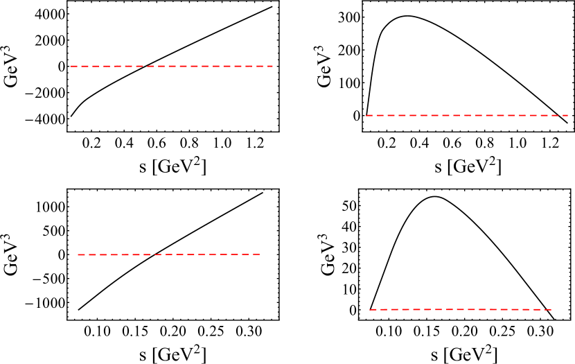
Figure 3: The $S$- (left) and $D$-wave (right) box amplitudes in $\Upsilon(4S)\to\Upsilon(1S)\pi^{+}\pi^{-}$ (top) and $\Upsilon(4S)\to\Upsilon(2S)\pi^{+}\pi^{-}$ (bottom). The black solid and red dashed lines denote the real and imaginary parts, respectively.

The partial-wave projection of the loop amplitude for the $\Upsilon(mS)\to\Upsilon(nS)PP$ process can be denoted as

$$\hat{M}_{l}^{\text{loop},P}(s)=g_{JHH(mS)}\,g_{JHH(nS)}\,\text{AmpBox}_{l}^{P}(s)\,.$$ (17)

The analytic expressions of $\text{AmpBox}_{l}^{P}(s)$ are very involved, so in Fig. 3 we only plot the numerical results for $\Upsilon(4S)\rightarrow\Upsilon(1S,2S)\pi^{+}\pi^{-}$ in the physical region. Note that the imaginary parts, which are due to the on-shell $B\bar{B}$ intermediate states, are tiny due to the smallness of phase space and the fact that the $B\bar{B}$ pair appears in a relative $P$-wave.

II.4 Final-state interactions with a dispersive approach, Omnès solution

There are strong FSIs in the $\pi\pi$ system especially in the isoscalar $S$-wave, which can be taken into account model-independently using dispersion theory. Based on the principles of unitarity and analyticity, dispersion theory determines the decay amplitudes up to some subtraction constants, which can be fixed by matching to the results of chiral effective theory. Since the mass difference between the $\Upsilon(4S)$ and the $\Upsilon(1S)$ is larger than the $K\bar{K}$ threshold, we will consider the isospin symmetric two-channel ($\pi\pi$ and $K\bar{K}$) FSI for the dominant $S$-wave component, while for the $D$-wave only single-channel $\pi\pi$ FSI will be considered.

For the $\Upsilon(mS)\rightarrow\Upsilon(nS)\pi^{+}\pi^{-}$ processes, the partial-wave expansion of the amplitude including FSI reads

$$\mathscr{M}^{\text{full}}(s,\cos\theta)=\epsilon_{\Upsilon(nS)}\cdot\epsilon_{\Upsilon(mS)}\sum_{l=0}^{\infty}\left[M_{l}^{\pi}(s)+\hat{M}_{l}^{\pi}(s)\right]P_{l}(\cos\theta)\,,$$ (18)

where $M_{l}^{\pi}(s)$ represents the right-hand cut part and accounts for $s$-channel rescattering, and the “hat functions” $\hat{M}_{l}^{\pi}(s)$ contain the left-hand cuts, contributed by crossed-channel pole terms or open-flavor loop effects. In general the box diagrams contribute to both the left-hand cuts at $t,u>(m_{B^{(*)}}+m_{B^{(*)}})^{2}$ and right-hand cut at $s>(m_{B^{(*)}}+m_{B^{(*)}})^{2}$, however, this right-hand cut is far away from the physical region, so it can be safely neglected. In this study, we approximate the left-hand cuts by the sum of the $Z_{b}$-exchange diagram and the box diagrams, $\hat{M}_{l}^{\pi}(s)=\hat{M}_{l}^{Z_{b},\pi}(s)+\hat{M}_{l}^{\text{loop},\pi}(s)$. Similar methods to approximate the left-hand-cut structures by including resonance exchange (in the case of no loops) have been applied in Refs. Moussallam-gamma ; KubisPlenter ; ZHGuo ; Kang .

Next we discuss the Omnès solution to obtain the amplitude including FSI. For simplicity first we discuss the single-channel solution, which applies for the $D$-wave case. The functions $\hat{M}_{l}(s)$ are real along the right-hand cut, so in the elastic $\pi\pi$ rescattering region the partial-wave unitarity conditions reads

$$\textrm{Im}\,M_{l}(s)=\left[M_{l}(s)+\hat{M}_{l}(s)\right]\sin\delta_{l}^{0}(s)e^{-i\delta_{l}^{0}(s)}\,.$$ (19)

In the elastic region, the phases $\delta_{l}^{I}$ of the partial-wave amplitudes of isospin $I$ and angular momentum $l$ equal the $\pi\pi$ elastic phase shifts modulo $n\pi$, as required by Watson’s theorem Watson1 ; Watson2 . The Omnès function is defined as Omnes

$$\Omega_{l}^{I}(s)=\exp\bigg{\{}\frac{s}{\pi}\int^{\infty}_{4m_{\pi}^{2}}\frac{{\text{d}}x}{x}\frac{\delta_{l}^{I}(x)}{x-s}\bigg{\}}\,,$$ (20)

which obeys $\Omega_{l}^{I}(s+i\epsilon)=e^{2i\delta_{l}^{I}}\Omega_{l}^{I}(s-i\epsilon)$. Using the Omnès function, the solution of Eq. (19) can be obtained Leutwyler96 ; Chen2016

$$M_{l}(s)=\Omega_{l}^{0}(s)\bigg{\{}P_{l}^{n-1}(s)+\frac{s^{n}}{\pi}\int_{4m_{\pi}^{2}}^{\infty}\frac{{\text{d}}x}{x^{n}}\frac{\hat{M}_{l}(x)\sin\delta_{l}^{0}(x)}{|\Omega_{l}^{0}(x)|(x-s)}\bigg{\}}\,,$$ (21)

where the polynomial $P_{l}^{n-1}(s)$ is a subtraction function. For the $D$-wave phase shift $\delta_{2}^{0}(s)$, we will use the result given by the Madrid–Kraków collaboration Pelaez , and smoothly continue it to $\pi$ for $s\to\infty$.

For the $S$-wave, we will take into account the two-channel rescattering effects. Along the right-hand cut, the two-channel unitarity conditions reads

$$\textrm{Im}\,\mathbf{M}_{0}(s)=2iT_{0}^{0\ast}(s)\Sigma(s)\left[\mathbf{M}_{0}(s)+\hat{\mathbf{M}}_{0}(s)\right]\,,$$ (22)

where the two-dimensional vectors $\mathbf{M}_{0}(s)$ and $\hat{\mathbf{M}}_{0}(s)$ contain the right-hand- and the left-hand-cut parts of both the $\pi\pi$ and the $K\bar{K}$ final states, respectively,

$$\mathbf{M}_{0}(s)=\left({\begin{array}[]{*{2}c}{M^{\pi}_{0}(s)}\\ {\frac{2}{\sqrt{3}}M^{K}_{0}(s)}\\ \end{array}}\right),\hskip 14.22636pt\hat{\mathbf{M}}_{0}(s)=\left({\begin{array}[]{*{2}c}{\hat{M}^{\pi}_{0}(s)}\\ {\frac{2}{\sqrt{3}}\hat{M}^{K}_{0}(s)}\\ \end{array}}\right)\,.$$ (23)

The two-dimensional matrices $T_{0}^{0}(s)$ and $\Sigma(s)$ are

$$T_{0}^{0}(s)=\left({\begin{array}[]{*{2}c}\frac{\eta_{0}^{0}(s)e^{2i\delta_{0}^{0}(s)}-1}{2i\sigma_{\pi}(s)}&|g_{0}^{0}(s)|e^{i\psi_{0}^{0}(s)}\\ |g_{0}^{0}(s)|e^{i\psi_{0}^{0}(s)}&\frac{\eta_{0}^{0}(s)e^{2i\left(\psi_{0}^{0}(s)-\delta_{0}^{0}(s)\right)}-1}{2i\sigma_{K}(s)}\\ \end{array}}\right)$$ (24)

and $\Sigma(s)\equiv\text{diag}\big{(}\sigma_{\pi}(s)\theta(s-4m_{\pi}^{2}),\sigma_{K}(s)\theta(s-4m_{K}^{2})\big{)}$. There are three input functions in the $T_{0}^{0}(s)$ matrix: the $\pi\pi$ $S$-wave isoscalar phase shift $\delta_{0}^{0}(s)$, for which we will use the result from the Roy equation analysis in Ref. Leutwyler2012 ; the $\pi\pi\to K\bar{K}$ $S$-wave amplitude $g_{0}^{0}(s)=|g_{0}^{0}(s)|e^{i\psi_{0}^{0}(s)}$ with modulus and phase, for which the results based on the Roy–Steiner approach in Ref. Moussallam2004 will be used. These inputs are used below the appearance of additional inelasticities from $4\pi$ intermediate states, namely up to $\sqrt{s_{0}}=1.3\,\text{GeV}$ (the $f_{0}(1370)$ resonance is known to have a significant coupling to $4\pi$ Olive:2016xmw ). Above $s_{0}$, the phases $\delta_{0}^{0}(s)$ and $\psi_{0}^{0}$ are guided smoothly to 2$\pi$ Moussallam2000

$$\delta(s)=2\pi+(\delta(s_{0})-2\pi)\frac{2}{1+(\frac{s}{s_{0}})^{3/2}}\,.$$ (25)

The inelasticity $\eta_{0}^{0}(s)$ in Eq. (24) is related to the modulus $|g_{0}^{0}(s)|$ by

$$\eta_{0}^{0}(s)=\sqrt{1-4\sigma_{\pi}(s)\sigma_{K}(s)|g_{0}^{0}(s)|^{2}\theta(s-4m_{K}^{2})}\,.$$ (26)

The numerical solution of the homogeneous two-channel unitarity relation

$$\textrm{Im}\,\Omega(s)=2iT_{0}^{0\ast}(s)\Sigma(s)\Omega(s),\hskip 28.45274pt\Omega(0)=\mathbbm{1}\,,$$ (27)

has been computed in Refs. Leutwyler90 ; Moussallam2000 ; Hoferichter:2012wf ; Daub . Using $\Omega(s)$, the solution of the inhomogeneous two-channel unitarity condition in Eq. (22) is given by

$$\mathbf{M}_{0}(s)=\Omega(s)\bigg{\{}\mathbf{P}^{n-1}(s)+\frac{s^{n}}{\pi}\int_{4m_{\pi}^{2}}^{\infty}\frac{{\text{d}}x}{x^{n}}\frac{\Omega^{-1}(x)T(x)\Sigma(x)\hat{\mathbf{M}}_{0}(x)}{x-s}\bigg{\}}\,.$$ (28)

To determine the required number of subtractions that guarantees the dispersive integrals in Eqs. (21) and (28) to converge, we need to investigate the high-energy behavior of the integrand. First it is known that for the single-channel Omnès function defined in Eq. (20), it falls off asymptotically as $s^{-k}$ if the phase shift $\delta_{l}^{I}(s)$ approaches $k\pi$ at high energies. Since the $D$-wave $\pi\pi$ phase shift, $\delta_{2}^{0}(s)$, reaches $\pi$ for high energies, we have $\Omega_{2}^{0}(s)\sim 1/s$ for large $s$. Second, the high-energy behavior of the two-channel Omnès function has been analyzed in Ref. Moussallam2000 , and the $1/s$ asymptotic behavior of $\Omega_{l}^{I}(s)$ is ensured by the asymptotic condition $\sum\delta_{l}^{I}(s)\geq 2\pi$ for $s\to\infty$, where $\sum\delta_{l}^{I}(s)$ is the sum of the eigen phase shifts. Third, we have checked that in an intermediate energy range of $1\,\text{GeV}^{2}\lesssim s\ll m_{\Upsilon}^{2}$, both the inhomogeneities contributed by the $Z_{b}$-exchange term and the box graphs term grow at most linearly in $s$. So we conclude that in the dispersive representations for $M_{2}(s)$ and $\mathbf{M}_{0}(s)$, three subtractions are sufficient to make the dispersive integrals convergent.

At low energies, the amplitudes $M_{2}(s)$ and $\mathbf{M}_{0}(s)$ should match to the results of chiral perturbation theory. Namely, in the limit of switching off the final-state interactions, $\Omega_{2}^{0}(s)=1$ and $\Omega(0)=\mathbbm{1}$, the subtraction functions agree with the chiral representations given in Eqs. (10) and (13). Since both $M_{0}^{\chi}(s)$ and $M_{2}^{\chi}(s)$ grow no faster than $\sim s^{2}$, they can be covered by the degree of the subtractions. Therefore, for the $D$-wave, the integral equation takes the form

$$M_{2}^{\pi}(s)=\Omega_{2}^{0}(s)\bigg{\{}M_{2}^{\chi,\pi}(s)+\frac{s^{3}}{\pi}\int_{4m_{\pi}^{2}}^{\infty}\frac{{\text{d}}x}{x^{3}}\frac{\hat{M}_{2}^{\pi}(x)\sin\delta_{2}^{0}(x)}{|\Omega_{2}^{0}(x)|(x-s)}\bigg{\}}\,.$$ (29)

For the $S$-wave, the integral equation reads

$$\mathbf{M}_{0}(s)=\Omega(s)\bigg{\{}\mathbf{M}_{0}^{\chi}(s)+\frac{s^{3}}{\pi}\int_{4m_{\pi}^{2}}^{\infty}\frac{{\text{d}}x}{x^{3}}\frac{\Omega^{-1}(x)T(x)\Sigma(x)\hat{\mathbf{M}}_{0}(x)}{x-s}\bigg{\}}\,,$$ (30)

where $\mathbf{M}^{\chi}_{0}(s)=\big{(}M_{0}^{\chi,\pi}(s),2/\sqrt{3}\,M_{0}^{\chi,K}(s)\big{)}^{T}$.

The differential decay width for $\Upsilon(mS)\rightarrow\Upsilon(nS)\pi^{+}\pi^{-}$ with respect to the $\pi\pi$ invariant mass and the helicity angle reads

$$\frac{{\text{d}}\Gamma}{{\text{d}}\sqrt{s}\,{\text{d}}\cos\theta}=\frac{\sqrt{s}\,\sigma_{\pi}|\mathbf{q}|}{128\pi^{3}m_{\Upsilon(mS)}^{2}}\left|M_{0}^{\pi}+\hat{M}_{0}^{\pi}+(M_{2}^{\pi}+\hat{M}_{2}^{\pi})P_{2}(\cos\theta)\right|^{2}\,.$$ (31)

III Phenomenological discussion

The experimental data considered in this work are the $\pi\pi$ invariant mass distributions of the $\Upsilon(4S)\rightarrow\Upsilon(1S,2S)\pi^{+}\pi^{-}$ decays measured by the BaBar BABAR2006 and Belle Collaborations Belle2009 .

The chiral coupling constants $c_{i}$ in Eq. (1) are different for the two decays $\Upsilon(4S)\rightarrow\Upsilon(1S)\pi^{+}\pi^{-}$ and $\Upsilon(4S)\rightarrow\Upsilon(2S)\pi^{+}\pi^{-}$, since there is no symmetry connecting the bottomonium states with different radial excitations. The mass difference between the two $Z_{b}$ states is much smaller than the difference between their masses and the $\Upsilon(lS)\pi$ $(l=1,2)$ thresholds as well as $m_{\Upsilon(4S)}-m_{\pi}$; they have the same quantum numbers and thus the same coupling structure as given by Eq. (3). So the $Z_{b}(10610)$ and $Z_{b}(10650)$ contributions are strongly correlated in the fit, and it is very difficult to distinguish their effects from each other in the processes studied in this work. Therefore we only use one $Z_{b}$, the $Z_{b}(10610)$, in our fit by setting $C_{nm,2}=0$ as in our previous analysis of $\Upsilon(3S)\to\Upsilon(1,2S)\pi\pi$ Chen2016 . For the input mass of the $Z_{b}(10610)$, we will use the heavy-quark spin symmetry conserving result given in Ref. Guo2016 . The value of $g_{JHH(4S)}$ is extracted from the measured open-bottom decay widths of the $\Upsilon(4S)$, $g_{JHH(4S)}=1.43\,\text{GeV}^{-3/2}$.

For each $\Upsilon(4S)\to\Upsilon(nS)\pi\pi$ $(n=1,2)$ process, the unknown parameters are $c_{1}$ and $c_{2}$ corresponding to the chiral contact $\Upsilon\Upsilon^{\prime}\Phi\Phi$ coupling, $C_{4n,1}$ related to the $Z_{b}$ exchange mechanism, and $g_{JHH(nS)}$ for the box diagrams. To illustrate the effects of the $Z_{b}$-exchange and the box graph mechanisms, we perform several fits by choosing different strategies. Fit I only includes the chiral contact $c_{i}$ terms; Fit II adds the $Z_{b}$-exchange terms to them. Fit III includes the chiral contact $c_{i}$ terms and the box diagrams, and finally Fit IV takes all of the contact $c_{i}$ terms, the $Z_{b}$ exchange, and the box diagrams into account. FSI is included in all fits.

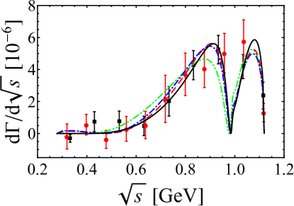
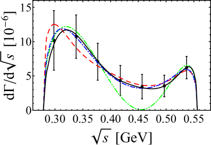
Figure 4: Fit results of the $\pi\pi$ invariant mass spectra for the decays $\Upsilon(4S)\to\Upsilon(1S)\pi^{+}\pi^{-}$ (left) and $\Upsilon(4S)\to\Upsilon(2S)\pi^{+}\pi^{-}$ (right). The solid squares and solid circles denote the data from the BaBar Collaboration BABAR2006 and Belle Collaboration Belle2009 , respectively. Fit I (green dash-dot-dotted): only including the chiral contact terms $c_{i}$, Fit II (red dashed): chiral contact terms and the $Z_{b}$-exchange term, Fit III (blue dot-dashed): chiral contact terms and box diagrams, Fit IV (black solid): including the contact terms $c_{i}$, the $Z_{b}$-exchange term, and the box diagrams. FSI is included in all fits.

In Fig. 4, the fitted results of Fits I–IV are shown as the green dash-dot-dotted, red dashed, blue dot-dashed, and black solid lines, respectively.

Table 2: Fit parameters from the best fits of the $\Upsilon(4S)\to\Upsilon(nS)\pi\pi$ $(n=1,2)$ processes.

	$~{}\Upsilon(4S)\to\Upsilon(1S)\pi^{+}\pi^{-}~{}$	$~{}\Upsilon(4S)\to\Upsilon(2S)\pi^{+}\pi^{-}~{}$
$c_{1}~{}[\text{GeV}^{-1}]$	$(9.8\pm 1.0)\times 10^{-4}$	$(1.2\pm 0.6)\times 10^{-1}$
$c_{2}~{}[\text{GeV}^{-1}]$	$(-1.6\pm 1.1)\times 10^{-4}$	$(-1.0\pm 0.6)\times 10^{-1}$
$C_{4n,1}$	$(2.6\pm 1.3)\times 10^{-4}$	$(-3.2\pm 1.8)\times 10^{-2}$
$g_{JHH(nS)}~{}[\text{GeV}^{-\frac{3}{2}}]$	$(8.6\pm 6.1)\times 10^{-5}$	$(1.7\pm 0.8)\times 10^{-2}$
${\chi^{2}}/{\rm d.o.f}$	${10.45}/{(20-4)}=0.65$	${0.04}/{(7-4)}=0.01$

The fitted parameters as well as the $\chi^{2}/\text{d.o.f.}$ of our best fit, Fit IV, are shown in Table 2. We find very different values for the parameters $c_{1}$ and $c_{2}$ from fitting the data of transitions between different $\Upsilon(lS)$ states. These low-energy constants parameterize the nonperturbative QCD matrix elements of gluonic operators between the initial and final bottomonia. For different initial and final $\Upsilon$ states, these parameters are not related to each other at the hadronic level, and can well be very different. In principle, the parameter values from the fit in this paper cannot be directly compared with those in Ref. Chen2016 , which do not include the box diagrams when analyzing the $\Upsilon(3S)$ and $\Upsilon(2S)$ dipion transitions. We thus made a new fit to the decay $\Upsilon(3S)\to\Upsilon(1S)\pi\pi$ studied therein. It turns out that the values of $c_{1}$ and $c_{2}$ decrease only by around 35% in comparison with those given in Table I of Ref. Chen2016 . Our fittings turn out to indicate the following hierarchy: $|c_{1,2}^{4\to 1}|\ll|c_{1,2}^{4\to 2}|\lesssim|c_{1,2}^{3\to 1}|\ll|c_{1,2}^{3\to 2}|$. This may be understood from the node structure of the $\Upsilon$ wave functions: for the processes with the same initial $\Upsilon$ state, the larger the difference between the principal quantum numbers, the smaller the gluonic matrix elements and thus the magnitude of the parameters. Note that the total $\chi^{2}$ value for the transition $\Upsilon(4S)\to\Upsilon(2S)\pi^{+}\pi^{-}$ is very low, $\chi^{2}/\text{d.o.f.}=0.01$. This small number reflects the observation that the fluctuation in the data appears to be significantly smaller than what the error bars allow for, which indicates that they might well be dominated by systematics.

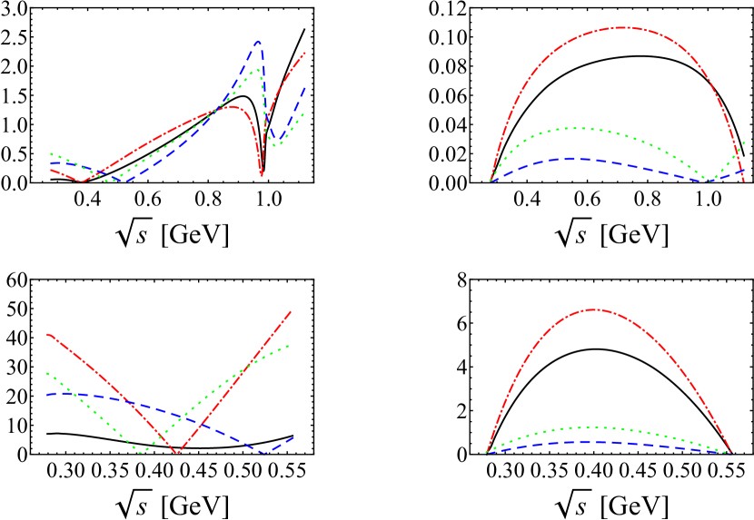
Figure 5: Moduli of the $S$- (left) and $D$-wave (right) amplitudes in $\Upsilon(4S)\to\Upsilon(1S)\pi^{+}\pi^{-}$ (top) and $\Upsilon(4S)\to\Upsilon(2S)\pi^{+}\pi^{-}$ (bottom). The black solid lines represent our best fit results, while the red dot-dashed, blue dashed, and green dotted lines correspond to the contributions from the $c_{i}$ terms, the $Z_{b}(10610)$, and the box diagrams, respectively.

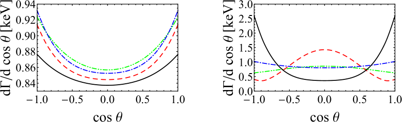
Figure 6: Theoretical predictions of the helicity angular distributions for the decays $\Upsilon(4S)\to\Upsilon(1S)\pi^{+}\pi^{-}$ (left) and $\Upsilon(4S)\to\Upsilon(2S)\pi^{+}\pi^{-}$ (right). The line style is as in Fig. 4.

Using the central values of the parameters in the best fit, in Fig. 5 we plot the moduli of the $S$- and $D$-wave amplitudes from the $c_{i}$ terms, the $Z_{b}(10610)$ state, and the box graphs for the processes $\Upsilon(4S)\to\Upsilon(1S)\pi^{+}\pi^{-}$ and $\Upsilon(4S)\to\Upsilon(2S)\pi^{+}\pi^{-}$, respectively. In addition, in Fig. 6 we show the resulting theoretical predictions for the angular distributions.

As shown in Fig. 4, including the $Z_{b}$-exchange and the box graph contributions improves the fit quality for $\Upsilon(4S)\to\Upsilon(1S)\pi^{+}\pi^{-}$ only marginally, mainly in the region around $1\,\text{GeV}$. However, for $\Upsilon(4S)\to\Upsilon(2S)\pi^{+}\pi^{-}$, the fit quality increases significantly when considering either of those two mechanisms (or both). Loop effects were already studied in the ${}^{3}P_{0}$ quark-pair-creation model in Ref. Kuang1991 , and found to be tiny for $\Upsilon(3S,2S)\to\Upsilon(2S,1S)\pi^{+}\pi^{-}$. This is probably due to the fact that $\Upsilon(3S,2S)$ are too far below the $B\bar{B}$ threshold. This situation is expected to change for the $\Upsilon(4S)$, with the open-bottom channels contributing significantly to its decay rate. In Fig. 5, one observes that for the dominant $S$-wave amplitudes, the contributions from the $c_{i}$ terms, from the $Z_{b}$-exchange term, and from the box diagram term are all of the same order. Especially, for the decay $\Upsilon(4S)\to\Upsilon(1S)\pi^{+}\pi^{-}$, the box graphs and the $Z_{b}$ exchange play a major role in the energy range around $0.95\,\text{GeV}$, and account for the better description of the data there. Note that the contribution of loops including $B_{s}$ mesons, producing kaons that subsequently rescatter into a pion pair, is entirely negligible: in the NREFT formalism, these graphs vanish at the $K\bar{K}$ threshold. For the $D$-wave, the contributions from $Z_{b}$ exchange and the box graphs are much smaller than that from the $c_{i}$ terms. We should mention that the plots in Fig. 5 correspond to using the central values of the best fit parameters. The shapes of the curves corresponding to the box diagrams and the $Z_{b}$-exchange terms are similar; however, their relative strength is not very meaningful because there is a strong correlation in the fit between the parameters $C_{41,1}$ and $J_{JHH(1S)}$. This can be easily seen from the fact that the curves for Fit II and Fit III are very similar to each other in Fig. 4 (left), which means that the $Z_{b}$-exchange and box terms can hardly be distinguished in the $\pi\pi$ invariant mass distribution of the transition $\Upsilon(4S)\to\Upsilon(1S)\pi^{+}\pi^{-}$.

Notice that in Refs. Meng2008 ; DYChen2011 , the loop contribution of the sequential process $\Upsilon(4S)\to B\bar{B}\to\Upsilon(nS)S\to\Upsilon(nS)\pi^{+}\pi^{-}(n=1,2)$, where the scalar $S$ can correspond to the $f_{0}(500)$ and the $f_{0}(980)$, has been considered. This kind of loop topology can be described by Fig. 2 (a) including FSIs, which is suppressed compared to the box graphs in NREFT. In our scheme, the FSIs are taken into account in a model-independent way, and we do not have to specify the contributing scalar resonances. Another merit of our calculation is that, instead of only obtaining the absorptive part of the loops by using Cutkosky rules Meng2008 ; DYChen2011 , we completely compute both their real and imaginary parts.

An interesting feature of the $\pi\pi$ invariant mass distribution of $\Upsilon(4S)\to\Upsilon(1S)\pi^{+}\pi^{-}$ is that the older Belle data from Ref. Belle2005 hint at a two-peak structure in the range of $m_{\pi^{+}\pi^{-}}=0.8\ldots 1.2\,\text{GeV}$, while the later measurements given in Refs. BABAR2006 ; Belle2009 do not display such a feature in any obvious way. As the mass difference between $\Upsilon(4S)$ and $\Upsilon(1S)$ is about $1.12\,\text{GeV}$, the isoscalar-scalar $f_{0}(980)$ meson, which couples strongly to $\pi\pi$, should be visible in the spectrum. With FSI described reliably in the dispersive approach, we see that the $f_{0}(980)$ indeed accounts for a dip at its mass, and a two-peak structure is naturally produced. A possible reason why such a two-peak structure is not observed in Refs. BABAR2006 ; Belle2009 may be the wide energy bins used in these experimental measurements. The fact that the $f_{0}(980)$ should be manifest in the $\pi\pi$ invariant mass distribution of $\Upsilon(4S)\to\Upsilon(1S)\pi^{+}\pi^{-}$ has already been emphasized in Ref. Guo2007:4S . The dip caused by the $f_{0}(980)$ is also present in the calculation of Ref. Surovtsev:2015hna .

For the $\Upsilon(4S)\to\Upsilon(2S)\pi^{+}\pi^{-}$ process, it is known that the two-hump behavior in the $\pi\pi$ invariant mass spectra is incompatible with the prediction from the QCD multipole expansion, resembling the case of $\Upsilon(3S)\to\Upsilon(1S)\pi\pi$ Kuang1991 ; Eichten2008 ; Chen2016 . In the formalism outlined above, the original formulation of the QCD multipole expansion appears by including only the tree-level $c_{i}$-terms, however, omitting the $\pi\pi$ FSIs. As shown by the blue dot-dashed line in the right panel of Fig. 4, including the final-state interaction can roughly reproduce a two-hump structure. However, it produces a zero in the amplitude inside the physical region and the agreement with the data is not very convincing. This feature was also observed in our previous study of $\Upsilon(3S)\to\Upsilon(1S)\pi\pi$, where, however, a simultaneous fit of the $\pi\pi$ invariant mass and the helicity angular distributions cannot reproduce the two-hump behavior in the dipion mass spectra by only using the $c_{i}$ terms Chen2016 . The angular distribution data are therefore important to distinguish the effects of different mechanisms. In Fig. 6, the theoretical predictions of the helicity angular distributions in different fit scenarios are shown. For $\Upsilon(4S)\to\Upsilon(2S)\pi^{+}\pi^{-}$, the angular distributions are distinctly different when including the $Z_{b}$-exchange and box graphs terms, hence these results can be used to check their effects when experimental data become available in the future.

Using the fit parameters given in Table 2, we can predict the decay width of $\Upsilon(4S)\rightarrow\Upsilon(1S)K^{+}K^{-}$, as well as the corresponding $K\bar{K}$ invariant mass distribution. The relevant Feynman diagrams can be obtained by replacing all external pions by kaons in Fig. 1, but without diagram (b1) due to the absence of a $Z_{b}\Upsilon K$ vertex. The $Z_{b}$ contributes also to $K\bar{K}$ through diagram (b2) due to the final-state interactions that, especially around the $K\bar{K}$ threshold, provides strong $\pi\pi\to K\bar{K}$ transitions. Most ingredients of the amplitude of the $\Upsilon(4S)\rightarrow\Upsilon(1S)K^{+}K^{-}$ process have been given in Sec. II. We omit the $K\bar{K}$ $D$-wave, which is negligible due to its strong near-threshold suppression. Within $1\sigma$ uncertainties, the prediction of the decay width of $\Upsilon(4S)\rightarrow\Upsilon(1S)K^{+}K^{-}$ is

$$\Gamma_{\Upsilon(4S)\rightarrow\Upsilon(1S)K^{+}K^{-}}=0.18_{-0.09}^{+0.21}\,\text{keV}\,,$$ (32)

corresponding to a branching fraction of $0.9^{+1.0}_{-0.4}\times 10^{-5}$, and the dikaon invariant mass spectrum is given in Fig. 7 (top left). The rapid rise of the $K\bar{K}$ invariant mass distribution in the near-threshold region is a result of the $f_{0}(980)$, in line with the dip around $1\,\text{GeV}$ in Fig. 4. Like the $\Upsilon(4S)\rightarrow\Upsilon(1S)\pi^{+}\pi^{-}$ process, there is a strong correlation between the $Z_{b}$-exchange terms and the box diagrams in the $\Upsilon(4S)\rightarrow\Upsilon(1S)K^{+}K^{-}$ process, and in Fig. 7 we also plot the contributions from the the $c_{i}$ terms (top right), the $Z_{b}(10610)$ state plus box graphs (bottom left), and their interference (bottom right), respectively. One finds that for the central values of the theoretical predictions, the $Z_{b}$-exchange term and the box graphs nearly cancel each other, and the total line shape is quite similar to the $c_{i}$ terms only. Both the rapid rise in the $m_{K\bar{K}}$ distribution and the nontrivial structure in the large $m_{\pi\pi}$ region of the dipion invariant mass distribution are due to the final-state interactions between the light mesons, depicted in Fig. 1 (c1, d1, a2, …, d2), which receive contributions from both the $Z_{b}$-exchange and box diagrams. As a result, their strong correlation in the fit to the data of the dipion transitions leads to the significant cancellation in the prediction of the $m_{K\bar{K}}$ distribution. The large spread mainly comes from the uncertainties of $Z_{b}(10610)$ plus box graphs, and the interference term. These predictions encourage future experimental measurements in this channel.

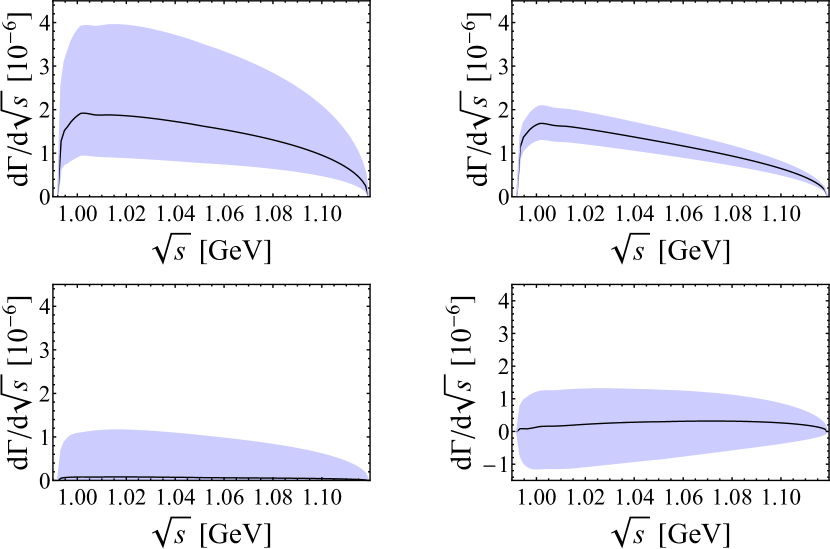
Figure 7: Theoretical prediction of the $K\bar{K}$ invariant mass spectrum for the decay $\Upsilon(4S)\to\Upsilon(1S)K^{+}K^{-}$ (top left). The contributions from the $c_{i}$ terms (top right), the $Z_{b}(10610)$ state plus box graphs (bottom left), and their interference (bottom right) are also depicted. The shaded areas corresponds to the error band.

IV Conclusions

We have studied the effects of $Z_{b}$ exchange and bottom meson loops in the decays $\Upsilon(4S)\to\Upsilon(nS)\pi\pi$ $(n=1,2)$. The bottom meson loops are treated in the NREFT scheme, in which the power counting rules indicate that the box diagrams are dominant. The strong FSIs, especially the coupled-channel FSI in the $S$-wave, are taken into account model-independently by using dispersion theory. The forms of the subtraction functions are obtained by matching to the leading chiral contact terms. Through fitting the data of the $\pi\pi$ invariant mass spectra, the couplings of the $\Upsilon\Upsilon^{\prime}\pi\pi$ and $\Upsilon B^{(*)}B^{(*)}$ vertices, as well as the product of couplings of the $Z_{b}\Upsilon\pi$ and $Z_{b}\Upsilon^{\prime}\pi$ vertices are determined (where $\Upsilon$ and $\Upsilon^{\prime}$ denote the final- and initial-state bottomonia). For the dominant $S$-wave component, it is found that the contributions from $Z_{b}$ exchange, the loops, and the chiral contact term are of the same order. For $\Upsilon(4S)\to\Upsilon(2S)\pi^{+}\pi^{-}$, including the $Z_{b}$-exchange term and the bottom meson loops naturally describes the two-hump behavior in the $\pi\pi$ invariant mass distribution. Unfortunately, the present data are insufficient to distinguish between the effects of the $Z_{b}$ exchange and the bottom meson loops. We provide theoretical predictions of the helicity angular distributions, which may be useful to identify the effects of $Z_{b}$-exchange and bottom meson loops with future experimental data. For the $\Upsilon(4S)\to\Upsilon(1S)\pi^{+}\pi^{-}$ decay, we expect that there is a dip in the $\pi\pi$ spectrum around $1\,\text{GeV}$, caused by the opening of the $K\bar{K}$ channel near the $f_{0}(980)$ resonance. This dip has probably not been observed yet in the present experimental data yet due to lack of sufficiently precise energy resolution. Improved data to resolve this issue is eagerly awaited. We also predict the decay width and the $K\bar{K}$ invariant mass distribution of the $\Upsilon(4S)\rightarrow\Upsilon(1S)K^{+}K^{-}$ process, demonstrating the usefulness of this additional measurement that should be feasible at Belle II.

Appendix A Remarks on the box diagrams and four-point integrals

In this appendix, we will discuss the calculation of the amplitudes that involve four-point loop integrals in some detail. We will start by discussing the parametrization and simplification of scalar four-point integrals. Then we will introduce a tensor reduction scheme to deal with higher-rank integrals. Finally, we will give the leading part of the corresponding integrals (proportional to $\bm{\epsilon}_{\Upsilon^{\prime}}\cdot\bm{\epsilon}_{\Upsilon}$) for the possible intermediate bottom mesons.

A.1 Scalar four-point integrals

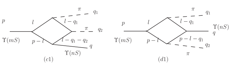
Figure 8: Kinematics used in the calculation of the four-point integrals.

Because of the simpler structure we begin with the first topology as shown in Fig. 8. The corresponding scalar integral, evaluated for the initial bottomonium at rest ($p=(M,\mathbf{0})$) and labelled $J^{(0c)}$ to be consistent with Fig. 1, reads

$$J^{(0c)} \equiv i\int\!\frac{d^{4}l}{(2\pi)^{4}}\frac{1}{[l^{2}-m_{1}^{2}+i\epsilon][(p-l)^{2}-m_{2}^{2}+i\epsilon][(l-q_{1}-q_{2})^{2}-m_{3}^{2}+i\epsilon][(l-q_{1})^{2}-m_{4}^{2}+i\epsilon]}$$

$$\simeq\frac{-i}{16m_{1}m_{2}m_{3}m_{4}}\int\!\frac{d^{4}l}{(2\pi)^{4}}\frac{1}{\left[l^{0}-\frac{\mathbf{l}^{2}}{2m_{1}}-m_{1}+i\epsilon\right]\left[l^{0}-M+\frac{\mathbf{l}^{2}}{2m_{2}}+m_{2}-i\epsilon\right]}$$

$$\times\frac{1}{\left[l^{0}-q_{1}^{0}-q_{2}^{0}-\frac{(\mathbf{l}+\mathbf{q})^{2}}{2m_{3}}-m_{3}+i\epsilon\right]\left[l^{0}-q_{1}^{0}-\frac{(\mathbf{l}-\mathbf{q}_{1})^{2}}{2m_{4}}-m_{4}+i\epsilon\right]}.$$ (33)

Performing the contour integration is straightforward since only one pole is located in the upper half-plane. We find

$$-\frac{\mu_{12}\mu_{23}\mu_{24}}{2m_{1}m_{2}m_{3}m_{4}}\int\!\frac{d^{3}l}{(2\pi)^{3}}\frac{1}{[\mathbf{l}^{2}+c_{12}-i\epsilon][\mathbf{l}^{2}+2\frac{\mu_{23}}{m_{3}}\mathbf{l}\cdot\mathbf{q}+c_{23}-i\epsilon][\mathbf{l}^{2}-2\frac{\mu_{24}}{m_{4}}\mathbf{l}\cdot\mathbf{q}_{1}+c_{24}-i\epsilon]},$$ (34)

where we defined

$$c_{12} \equiv 2\mu_{12}\left(m_{1}+m_{2}-M\right),\quad c_{23}\equiv 2\mu_{23}\left(m_{2}+m_{3}-M+q_{1}^{0}+q_{2}^{0}+\frac{\mathbf{q}^{2}}{2m_{3}}\right),$$

$$c_{24} \equiv 2\mu_{24}\left(m_{2}+m_{4}-M+q^{0}_{1}+\frac{\mathbf{q}_{1}^{2}}{2m_{4}}\right),\quad\mu_{ij}=\frac{m_{i}m_{j}}{m_{i}+m_{j}}.$$ (35)

For the second topology we immediately find

$$J^{(0d)} \equiv i\int\!\frac{d^{4}l}{(2\pi)^{4}}\frac{1}{[l^{2}-m_{1}^{2}+i\epsilon][(p-l)^{2}-m_{2}^{2}+i\epsilon][(p-q_{2}-l)^{2}-m_{3}^{2}+i\epsilon][(l-q_{1})^{2}-m_{4}^{2}+i\epsilon]}$$

$$\simeq\frac{-i}{16m_{1}m_{2}m_{3}m_{4}}\int\!\frac{d^{4}l}{(2\pi)^{4}}\frac{1}{\left[l^{0}-\frac{\mathbf{l}^{2}}{2m_{1}}-m_{1}+i\epsilon\right]\left[l^{0}-M+\frac{\mathbf{l}^{2}}{2m_{2}}+m_{2}-i\epsilon\right]}$$

$$\times\frac{1}{\left[l^{0}+q_{2}^{0}-M+\frac{(\mathbf{l}+\mathbf{q}_{2})^{2}}{2m_{3}}+m_{3}-i\epsilon\right]\left[l^{0}-q_{1}^{0}-\frac{(\mathbf{l}-\mathbf{q}_{1})^{2}}{2m_{4}}-m_{4}+i\epsilon\right]}.$$ (36)

Here the possibility for two different cuts to go on-shell leads to a slightly more complicated three-dimensional integral

$$-\frac{\mu_{12}\mu_{34}}{2m_{1}m_{2}m_{3}m_{4}}\int\!\frac{d^{3}l}{(2\pi)^{3}}\frac{1}{[\mathbf{l}^{2}+d_{12}-i\epsilon][\mathbf{l}^{2}-2\frac{\mu_{34}}{m_{4}}\mathbf{l}\cdot\mathbf{q}_{1}-2\frac{\mu_{34}}{m_{3}}\mathbf{l}\cdot\mathbf{q}_{2}+d_{34}-i\epsilon]}$$

$$\times\left[\frac{\mu_{24}}{[\mathbf{l}^{2}-2\frac{\mu_{24}}{m_{4}}\mathbf{l}\cdot\mathbf{q}_{1}+d_{24}-i\epsilon]}+\frac{\mu_{13}}{[\mathbf{l}^{2}+2\frac{\mu_{13}}{m_{3}}\mathbf{l}\cdot\mathbf{q}_{2}+d_{13}-i\epsilon]}\right],$$ (37)

where we defined

$$d_{12} \equiv 2\mu_{12}\left(m_{1}+m_{2}-M\right), d_{34} \equiv 2\mu_{34}\left(m_{3}+m_{4}-q^{0}+\frac{\mathbf{q}_{1}^{2}}{2m_{4}}+\frac{\mathbf{q}_{2}^{2}}{2m_{3}}\right),$$

$$d_{24} \equiv 2\mu_{24}\left(m_{2}+m_{4}-M+q_{1}^{0}+\frac{\mathbf{q}_{1}^{2}}{2m_{4}}\right), d_{13} \equiv 2\mu_{13}\left(m_{1}+m_{3}-M+q_{2}^{0}+\frac{\mathbf{q}_{2}^{2}}{2m_{3}}\right).$$ (38)

In both cases the remaining three-dimensional momentum integration needs to be carried out numerically.

A.2 Tensor reduction

Since each of the interactions of an $\Upsilon$ with a pair of bottom mesons scales with the momentum of the latter we will have to deal with

$$\frac{-\mu_{12}\mu_{23}\mu_{24}}{2m_{1}m_{2}m_{3}m_{4}}\int\!\frac{d^{3}l}{(2\pi)^{3}}\frac{f(l)}{[\mathbf{l}^{2}+c_{12}-i\epsilon][\mathbf{l}^{2}+2\frac{\mu_{23}}{m_{3}}\mathbf{l}\cdot\mathbf{q}+c_{23}-i\epsilon][\mathbf{l}^{2}-2\frac{\mu_{24}}{m_{4}}\mathbf{l}\cdot\mathbf{q}_{1}+c_{24}-i\epsilon]},$$ (39)

where $f(l)=\{1,\,l^{i},\,l^{i}l^{j}\}$ for the fundamental scalar, vector, and tensor integrals, respectively. Using the momentum of the final state $\Upsilon$, $\mathbf{q}$, and $\mathbf{q}_{\perp}=\mathbf{q}_{1}-\mathbf{q}(\mathbf{q}\cdot\mathbf{q}_{1})/\mathbf{q}^{2}$, a convenient parametrization reads

$$J^{(1)i} =\frac{-\mu_{12}\mu_{23}\mu_{24}}{2m_{1}m_{2}m_{3}m_{4}}\int\!\frac{d^{3}l}{(2\pi)^{3}}\frac{l^{i}}{[\mathbf{l}^{2}+c_{1}-i\epsilon][\mathbf{l}^{2}-2\frac{\mu_{23}}{m_{3}}\mathbf{l}\cdot\mathbf{q}+c_{2}-i\epsilon][\mathbf{l}^{2}-2\frac{\mu_{24}}{m_{4}}\mathbf{l}\cdot\mathbf{q}_{1}+c_{3}-i\epsilon]}$$

$$\equiv q^{i}J_{1}^{(1c)}+q_{\perp}^{i}J_{2}^{(1c)}$$ (40)

and

$$J^{(2)ij} =\frac{-\mu_{12}\mu_{23}\mu_{24}}{2m_{1}m_{2}m_{3}m_{4}}\int\!\frac{d^{3}l}{(2\pi)^{3}}\frac{l^{i}l^{j}}{[\mathbf{l}^{2}+c_{1}-i\epsilon][\mathbf{l}^{2}-2\frac{\mu_{23}}{m_{3}}\mathbf{l}\cdot\mathbf{q}+c_{2}-i\epsilon][\mathbf{l}^{2}-2\frac{\mu_{24}}{m_{4}}\mathbf{l}\cdot\mathbf{q}_{1}+c_{3}-i\epsilon]}$$

$$\equiv\left(\delta^{ij}-\frac{q^{i}q^{j}}{\mathbf{q}^{2}}-\frac{q_{\perp}^{i}q_{\perp}^{j}}{\mathbf{q}_{\perp}^{2}}\right)J_{0}^{(2c)}+\frac{q^{i}q^{j}}{\mathbf{q}^{2}}J_{1}^{(2c)}+\frac{q_{\perp}^{i}q_{\perp}^{j}}{\mathbf{q}_{\perp}^{2}}J_{2}^{(2c)}+\frac{q^{i}q_{\perp}^{j}+q_{\perp}^{i}q^{j}}{|\mathbf{q}||\mathbf{q}_{\perp}|}J_{3}^{(2c)},$$ (41)

where the scalar integrals $J^{(r)}_{m}$ can easily be disentangled and have to be evaluated numerically. The corresponding expressions for topology II can be obtained by changing the denominators accordingly.

A.3 Amplitudes

Intermediate mesons	Amplitude
$[P,P,P,V]$	$8q_{1}\cdot q_{2}J^{(2)ab}$
$[P,V,P,V]$	$-8q_{1}\cdot q_{2}J^{(2)ab}$
$[V,P,V,P]$	$4\delta^{ab}q_{1}^{i}\left(2q_{2}^{j}J^{(2)ij}+q\cdot q_{2}J^{(1)i}\right)$
$[P,V,V,V]$	$4\delta^{ab}\left(q_{1}^{i}q\cdot q_{2}-q_{2}^{i}q\cdot q_{1}\right)J^{(1)i}$
$[V,P,V,V]$	$4\delta^{ab}q_{1}^{i}\left(2q_{2}^{j}J^{(2)ij}+q\cdot q_{2}J^{(1)i}\right)$
$[V,V,P,V]$	$4\delta^{ab}\left(q_{1}^{i}q\cdot q_{2}-q_{2}^{i}q\cdot q_{1}\right)J^{(1)i}$
$[V,V,V,P]$	$8\delta^{ai}\delta^{bj}q_{1}\cdot q_{2}J^{(2)ij}+4\delta^{ab}q_{1}^{i}\left(2q_{2}^{j}J^{(2)ij}+q\cdot q_{2}J^{(1)i}\right)$
$[V,V,V,V]$	$4\delta^{ab}\left(4\delta^{ij}q_{1}\cdot q_{2}J^{(2)ij}-q_{2}^{i}q\cdot q_{1}J^{(1)i}+q_{1}^{i}\left(q\cdot q_{2}J^{(1)i}-4q_{2}^{j}J^{(2)ij}\right)\right)$

Table 3: All loops contributing to topology (c1) in Fig. 1. The mesons are listed as $[M1,M2,M3,M4]$, $P$ and $V$ denote intermediate pseudoscalar and vector mesons, respectively. The different flavors are dropped for simplicity—the full amplitude contains the sum of all possible ones.

Tables 3 and 4 list the relevant amplitudes for this calculation. We will only give the dominant amplitudes, i.e. the ones that contribute to the part proportional to $\epsilon(\Upsilon^{\prime})\cdot\epsilon(\Upsilon)$ as was explained in the main text. We further notice that all box diagrams are proportional to the overall factor $\epsilon^{a}(\Upsilon^{\prime})\,\epsilon^{b}(\Upsilon)\,g_{\pi}^{2}\,g_{J^{\prime}HH}\,g_{JHH}/F_{\pi}^{2}$.

Finally, we need to consider the different flavors of the intermediate bottom mesons. For topology (c1) with a pair of charged pions four possibilities exist: $[B^{(*)+},B^{(*)-},B^{(*)+},B^{(*)0}]$, $[B^{(*)-},B^{(*)+},B^{(*)-},{\bar{B}}^{(*)0}]$, $[B^{(*)0},{\bar{B}}^{(*)0},B^{(*)0},B^{(*)+}]$, and $[{\bar{B}}^{(*)0},B^{(*)0},{\bar{B}}^{(*)0},B^{(*)-}]$. For topology (d1) this reduces to just two: $[B^{(*)+},B^{(*)-},{\bar{B}}^{(*)0},B^{(*)0}]$ and $[{\bar{B}}^{(*)0},B^{(*)0},B^{(*)+},{\bar{B}}^{(*)-}]$. For the case of neutral pions the number of possible diagrams doubles—a factor 2 that is balanced by the factor $\sqrt{2}$ in the $SU(3)$ light-meson matrix.

Intermediate mesons	Amplitude
$[P,P,V,V]$	$8q_{1}\cdot q_{2}J^{(2)ab}$
$[P,V,P,V]$	$4\delta^{ab}\left(q_{1}\cdot q_{2}\left(2\delta^{ij}J^{(2)ij}+q_{2}^{i}J^{(1)i}\right)-q_{1}^{i}\left(2q_{2}^{j}J^{(2)ij}+q_{2}{}^{2}J^{(1)i}\right)\right)-8\delta^{ai}\delta^{bj}q_{1}\cdot q_{2}J^{(2)ij}$
$[V,V,P,P]$	$4\delta^{ab}q_{1}^{i}\left(2q_{2}^{j}J^{(2)ij}+q\cdot q_{2}J^{(1)i}\right)$
$[V,P,V,P]$	$4\delta^{ab}q_{1}^{i}\left(\left(q\cdot q_{2}+2q_{1}\cdot q_{2}\right)J^{(1)i}-2q_{2}^{j}J^{(2)ij}\right)$
$[P,V,V,V]$	$-4\delta^{ab}\left(2q_{1}^{i}q_{2}^{j}J^{(2)ij}+q_{2}^{i}\left(q_{1}\cdot q_{2}-q_{1}{}^{2}\right)J^{(1)i}\right)$
$[V,P,V,V]$	$-4\delta^{ab}q_{1}^{i}\left(2q_{2}^{j}J^{(2)ij}-\left(q\cdot q_{2}+2q_{1}\cdot q_{2}\right)J^{(1)i}\right)$
$[V,V,P,V]$	$-4\delta^{ab}\left(2q_{1}^{i}q_{2}^{j}J^{(2)ij}+q_{2}^{i}\left(q_{1}\cdot q_{2}-q_{1}{}^{2}\right)J^{(1)i}\right)$
$[V,V,V,P]$	$-4\delta^{ab}q_{1}^{i}\left(2q_{2}^{j}J^{(2)ij}+\left(q_{2}{}^{2}-q_{1}\cdot q_{2}\right)J^{(1)i}\right)$
$[V,V,V,V]$	$4\delta^{ab}\left(4\delta^{ij}q_{1}\cdot q_{2}J^{(2)ij}-q_{2}^{i}q\cdot q_{1}J^{(1)i}+q_{1}^{i}\left(q\cdot q_{2}J^{(1)i}-4q_{2}^{j}J^{(2)ij}\right)\right)$

Table 4: All loops contributing to topology (d1) in Fig. 1; see Table 3 for further notation.

References

• (1) M. B. Voloshin and V. I. Zakharov, Phys. Rev. Lett.  45, 688 (1980).
• (2) V. A. Novikov and M. A. Shifman, Z. Phys. C 8, 43 (1981).
• (3) Y. P. Kuang and T. M. Yan, Phys. Rev. D 24, 2874 (1981).
• (4) Y. P. Kuang, Front. Phys. China 1, 19 (2006) [hep-ph/0601044].
• (5) E. Eichten, S. Godfrey, H. Mahlke, and J. L. Rosner, Rev. Mod. Phys.  80, 1161 (2008) [hep-ph/0701208].
• (6) F.-K. Guo, P.-N. Shen, H.-C. Chiang, and R.-G. Ping, Nucl. Phys. A 761, 269 (2005) [hep-ph/0410204].
• (7) F.-K. Guo, P.-N. Shen, H.-C. Chiang, and R.-G. Ping, Phys. Lett. B 658, 27 (2007) [hep-ph/0601120].
• (8) Y.-H. Chen, J. T. Daub, F.-K. Guo, B. Kubis, U.-G. Meißner, and B.-S. Zou Phys. Rev. D 93, 034030 (2016) [arXiv:1512.03583 [hep-ph]].
• (9) I. Adachi [Belle Collaboration], arXiv:1105.4583 [hep-ex].
• (10) A. Bondar et al. [Belle Collaboration], Phys. Rev. Lett.  108, 122001 (2012) [arXiv:1110.2251 [hep-ex]].
• (11) M. B. Voloshin, JETP Lett.  37, 69 (1983) [Pisma Zh. Eksp. Teor. Fiz.  37, 58 (1983)].
• (12) V. V. Anisovich, D. V. Bugg, A. V. Sarantsev, and B.-S. Zou, Phys. Rev. D 51, R4619 (1995).
• (13) A. E. Bondar, R. V. Mizuk, and M. B. Voloshin, arXiv:1610.01102 [hep-ph].
• (14) F.-K. Guo, C. Hanhart, and U.-G. Meißner, Phys. Rev. Lett.  103, 082003 (2009); 104, 109901(E) (2010) [arXiv:0907.0521 [hep-ph]].
• (15) F.-K. Guo, C. Hanhart, G. Li, U.-G. Meißner, and Q. Zhao, Phys. Rev. D 83, 034013 (2011) [arXiv:1008.3632 [hep-ph]].
• (16) M. Cleven, Q. Wang, F.-K. Guo, C. Hanhart, U.-G. Meißner, and Q. Zhao, Phys. Rev. D 87, 074006 (2013) [arXiv:1301.6461 [hep-ph]].
• (17) T. Mannel and R. Urech, Z. Phys. C 73, 541 (1997) [hep-ph/9510406].
• (18) M. Cleven, F.-K. Guo, C. Hanhart, and U.-G. Meißner, Eur. Phys. J. A 47, 120 (2011) [arXiv:1107.0254 [hep-ph]].
• (19) S. Fleming and T. Mehen, Phys. Rev. D 78, 094019 (2008) [arXiv:0807.2674 [hep-ph]].
• (20) G. Burdman and J. F. Donoghue, Phys. Lett.  B 280, 287 (1992).
• (21) M. B. Wise, Phys. Rev.  D 45, R2188 (1992).
• (22) T. M. Yan, H. Y. Cheng, C. Y. Cheung, G. L. Lin, Y. C. Lin, and H. L. Yu, Phys. Rev.  D 46, 1148 (1992); 55, 5851(E) (1997).
• (23) R. Casalbuoni, A. Deandrea, N. Di Bartolomeo, R. Gatto, F. Feruglio, and G. Nardulli, Phys. Rept.  281, 145 (1997) [arXiv:hep-ph/9605342].
• (24) F. Bernardoni et al. [ALPHA Collaboration], Phys. Lett. B 740, 278 (2015) [arXiv:1404.6951 [hep-lat]].
• (25) I. W. Stewart, Nucl. Phys. B 529, 62 (1998) [hep-ph/9803227].
• (26) J. Hu and T. Mehen, Phys. Rev. D 73, 054003 (2006) [hep-ph/0511321].
• (27) T. Mehen and J. W. Powell, Phys. Rev. D 88, 034017 (2013) [arXiv:1306.5459 [hep-ph]].
• (28) R. García-Martín and B. Moussallam, Eur. Phys. J. C 70, 155 (2010) [arXiv:1006.5373 [hep-ph]].
• (29) B. Kubis and J. Plenter, Eur. Phys. J. C 75, 283 (2015) [arXiv:1504.02588 [hep-ph]].
• (30) Z.-H. Guo and J. A. Oller, Phys. Rev. D 84, 034005 (2011) [arXiv:1104.2849 [hep-ph]].
• (31) X.-W. Kang, B. Kubis, C. Hanhart, and U.-G. Meißner, Phys. Rev. D 89, 053015 (2014) [arXiv:1312.1193 [hep-ph]].
• (32) K. M. Watson, Phys. Rev.  88, 1163 (1952).
• (33) K. M. Watson, Phys. Rev.  95, 228 (1954).
• (34) R. Omnès, Nuovo Cim.  8, 316 (1958).
• (35) A. V. Anisovich and H. Leutwyler, Phys. Lett. B 375, 335 (1996) [hep-ph/9601237].
• (36) R. García-Martín, R. Kamiński, J. R. Peláez, J. Ruiz de Elvira, and F. J. Ynduráin, Phys. Rev.  D 83, 074004 (2011) [arXiv:1102.2183 [hep-ph]].
• (37) I. Caprini, G. Colangelo, and H. Leutwyler, Eur. Phys. J. C 72, 1860 (2012) [arXiv:1111.7160 [hep-ph]].
• (38) P. Büttiker, S. Descotes-Genon, and B. Moussallam, Eur. Phys. J. C 33, 409 (2004) [hep-ph/0310283].
• (39) C. Patrignani et al. [Particle Data Group Collaboration], Chin. Phys. C 40, 100001 (2016).
• (40) B. Moussallam, Eur. Phys. J. C 14, 111 (2000) [hep-ph/9909292].
• (41) J. F. Donoghue, J. Gasser, and H. Leutwyler, Nucl. Phys. B 343, 341 (1990).
• (42) M. Hoferichter, C. Ditsche, B. Kubis, and U.-G. Meißner, J. High Energy Phys. 06 (2012) 063 [arXiv:1204.6251 [hep-ph]].
• (43) J. T. Daub, C. Hanhart, and B. Kubis, J. High Energy Phys. 02 (2016) 009 [arXiv:1508.06841 [hep-ph]].
• (44) B. Aubert et al. [BaBar Collaboration], Phys. Rev. Lett.  96, 232001 (2006) [hep-ex/0604031].
• (45) A. Sokolov et al. [Belle Collaboration], Phys. Rev. D 79, 051103 (2009) [arXiv:0901.1431 [hep-ex]].
• (46) F.-K. Guo, C. Hanhart, Yu. S. Kalashnikova, P. Matuschek, R. V. Mizuk, A. V. Nefediev, Q. Wang, and J.-L. Wynen, Phys. Rev. D 93, 074031 (2016) [arXiv:1602.00940 [hep-ph]].
• (47) H. Y. Zhou and Y. P. Kuang, Phys. Rev. D 44, 756 (1991).
• (48) C. Meng and K.-T. Zhao, Phys. Rev. D 77, 074003 (2008) [arXiv:0712.3595 [hep-ph]].
• (49) D.-Y. Chen, X. Liu, and X.-Q. Li, Eur. Phys. J. C 71, 1808 (2011) [arXiv:1109.1406 [hep-ph]].
• (50) K. Abe et al. [Belle Collaboration], hep-ex/0512034.
• (51) Y. S. Surovtsev, P. Bydžovský, T. Gutsche, R. Kamiński, V. E. Lyubovitskij, and M. Nagy, Phys. Rev. D 92, 036002 (2015) [arXiv:1506.03023 [hep-ph]].