Two-dimensionalization of the flow driven by a slowly rotating impeller in a rapidly rotating fluid

Abstract

We characterize the two-dimensionalization process in the turbulent flow produced by an impeller rotating at a rate $\omega$ in a fluid rotating at a rate $\Omega$ around the same axis for Rossby number $Ro=\omega/\Omega$ down to $10^{-2}$. The flow can be described as the superposition of a large-scale vertically invariant global rotation and small-scale shear layers detached from the impeller blades. As $Ro$ decreases, the large-scale flow is subjected to azimuthal modulations. In this regime, the shear layers can be described in terms of wakes of inertial waves traveling with the blades, originating from the velocity difference between the non-axisymmetric large-scale flow and the blade rotation. The wakes are well defined and stable at low Rossby number, but they become disordered at $Ro$ of order of 1. This experiment provides insight into the route towards pure two-dimensionalization induced by a background rotation for flows driven by a non-axisymmetric rotating forcing.

I Introduction

A key feature of rapidly rotating flows is the tendency towards two-dimensionalization, a result known as the Taylor-Proudman theorem GreenspanBook ; DavidsonBook2013 ; Godeferd2015 . For asymptotically large rotation rates $\Omega$, this theorem states that the fluid motion with characteristic time much larger than the rotation period $\Omega^{-1}$, called geostrophic flow, is two-dimensional, invariant along the rotation axis (hereafter called vertical by convention). For large Reynolds number and moderate to small Rossby number (which compares the rotation period $\Omega^{-1}$ to the turbulent turnover time), such slow, large-scale, geostrophic flow may coexist with fast, three-dimensional fluctuations in the form of inertial waves Leoni2014 ; Yarom2014 ; Campagne2015 . Inertial waves are anisotropic, circularly polarized dispersive waves that propagate because of the restoring nature of the Coriolis force GreenspanBook ; McEwan1970 ; Machicoane2015 .

It was recently demonstrated by Gallet Gallet2015 that two-dimensionality can be reached exactly provided that the Rossby number is smaller than a Reynolds-number-dependent critical value. However, for most laboratory experiments, numerical simulations and geophysical flows, the Rossby number is moderate, $Ro\simeq 10^{-2}-1$, and the system is generally far from this asymptotic two-dimensional state Pedlosky1987 ; Vallis . This departure from two-dimensionality cannot be neglected in general: although most of the kinetic energy is carried by the geostrophic flow, three-dimensional fluctuations still remain responsible of most of the energy dissipation Campagne2015 ; Baqui2015 .

A question of practical interest is, for given initial or boundary conditions, to what extent a turbulent flow in a rotating frame is two-dimensional, and how the amount of two-dimensionality depends on the Reynolds and Rossby numbers. This question has received much attention, both experimentally Yarom2013 ; Campagne2014 ; Campagne2015 and numerically Bourouiba2012 ; Teitelbaum2012 ; Deusebio2014 ; Delache2014 ; Alexakis2015 . Recently, we introduced a simple configuration to address this question: it consists of an impeller rotating at a rate $\omega$ in a fluid under global rotation around the same axis at a rate $\Omega$. This configuration was first characterized at moderate to large Rossby number, $Ro=\omega/\Omega>2$, in Campagne et al. Campagne2016 , showing a strong two-dimensionalization of the mean flow associated with a reduction in turbulence intensity, and hence in turbulent drag, as $Ro$ is decreased below $\simeq O(10)$. The aim of the present paper is to explore the route towards two-dimensionality in this flow at much smaller Rossby number, down to $Ro\simeq 10^{-2}$.

A closely related configuration to investigate the transition towards two-dimensionality at low Rossby number, considered first in the pioneering work of Hide and Titman hide_titman , consists in spinning a disk in a rotating cylindrical container. At sufficiently low Rossby number, apart from boundaries, the flow is divided in two domains in solid-body rotation at angular velocity $\Omega+\omega$ (inside the cylinder tangential to the disk) and $\Omega$ (outside this cylinder), separated by a Stewartson shear layer Stewartson1957 . As the Rossby number is further decreased, this shear layer becomes unstable with respect to azimuthal modulations of increasing mode order $m$ Busse1968 . This instability, often referred to as barotropic Vallis , is generically observed in flows forced by a purely axisymmetric small differential rotation in a rapidly rotating system, in cylindrical niino1984 ; Dolzhanskii1990 ; konijnenberg ; fruh_read or spherical Hollerbach2003 ; Schaeffer2005 geometries.

The situation is more complex for a non-axisymmetric forcing, as the impeller considered here. First, the natural mode of the barotropic instability may be modified by the symmetry of the forcing (typically the number of blades for an impeller). Second, the non-axisymmetric “topography” of the forcing may be sources of inertial waves, which may delay the transition towards pure geostrophy. When excited by a disturbance moving at constant velocity, these inertial waves interfere and may form a stationary wake traveling with the disturbance Lighthill1967 ; peat1976 . In our experiment we find that, in the case of a rotating impeller, the wakes of inertial waves attached to each blade interact and produce small-scale fluctuations superimposed to the large-scale geostrophic flow, making the 2D transition in such flow richer than for a purely axisymmetric forcing.

The paper is organized as follows. Section II describes the experimental setup and particle image velocimetry measurements. The large-scale flow and the azimuthal instability as the Rossby number is decreased are described in Sec. III. The dynamics of the small-scale fluctuations are analyzed in Sec. IV. We show in particular that they can be described in terms of wakes of inertial waves generated by the velocity difference between the blades and the large-scale geostrophic flow.

II Experimental setup

The experimental setup, sketched in Fig. 1, is similar to the one described in Campagne et al. Campagne2016 , and is only briefly discussed here. A four-parallelepipedic-blade impeller rotates at a rate $\omega=0.5-90$ rpm around the vertical axis in a water-filled tank of $45\times 45$ cm² square base and 55 cm height. The impeller radius is $R=12$ cm, and each blade has a height $h=3.2$ cm and a thickness $e=0.5$ cm. The whole system is mounted on a platform rotating at a rate $\Omega$ in the range $4-30$ rpm. We restrict ourselves to the regime of cyclonic rotation, i.e. when the impeller rotates in the same direction as the platform. The Rossby number, defined as $Ro=\omega/\Omega$, covers the range $0.017-3.5$, much lower than the range $2-500$ covered in Ref. Campagne2016 . The Reynolds number $Re=\omega R^{2}/\nu$ (with $\nu$ the kinematic viscosity) is in the range $10^{3}-10^{5}$.

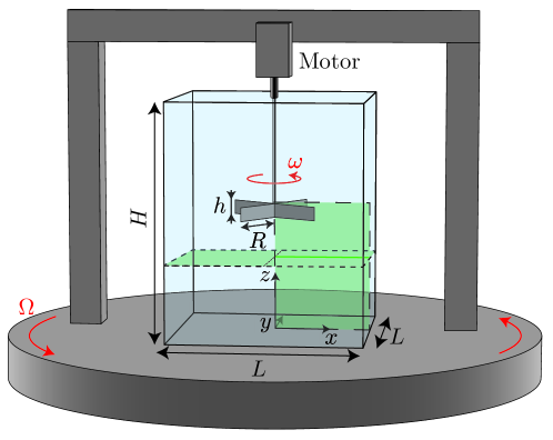
Figure 1: Experimental setup: a motor drives an impeller at a constant rotation rate $\omega$ in a water-filled tank mounted on a platform rotating at a rate $\Omega$ (in the laboratory frame, the impeller spins at a rate $\omega+\Omega$). PIV measurements are performed in the rotating frame, in a vertical or horizontal plane shown by the green areas. $H=55$ cm; $L=45$ cm; $h=3.2$ cm; $R=12$ cm.

We perform velocity measurements using a 2D particle image velocimetry (PIV) system mounted on the rotating platform, either in a vertical or a horizontal plane (green areas in Fig. 1). In the vertical configuration, the laser sheet contains the impeller axis, and the imaged plane covers a little more than one quarter of the tank section. In this configuration, 4 000 pairs of images of particles, separated by a time lag chosen between $1$ and $29$ ms within a pair, are acquired with a $2\,360\times 1\,776$ pixels camera at 10 Hz. Cross-correlation within pairs of images produces velocity fields sampled on a grid of $146\times 111$ points, with a spatial resolution of 2.1 mm. In the horizontal configuration, the laser sheet is located 10 cm below the impeller and almost the whole tank section is imaged. Between 1 500 and 15 000 images of particles are acquired at a rate from 3 to 30 Hz. Cross-correlation between successive images yields velocity fields sampled on $120\times 102$ points with a resolution of 3.6 mm.

III Large-scale geostrophic flow

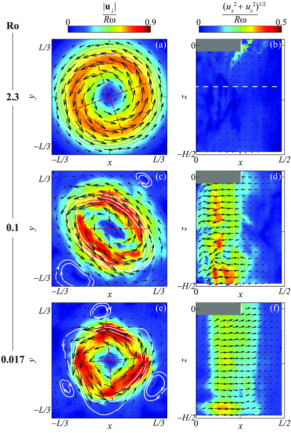
Figure 2: Flow structure for decreasing Rossby number ($Ro=2.3$, $0.1$ and $0.017$). Left column: instantaneous horizontal velocity field and streamlines in the horizontal plane, 10 cm below the impeller; colormap shows the norm $|\mathbf{u_{\perp}}|=\sqrt{u_{x}^{2}+u_{y}^{2}}$; the red dashed lines show the position of the blades located 10 cm above. Right column: instantaneous velocity field in the vertical plane $y=0$; colormap shows the norm $\sqrt{u_{x}^{2}+u_{z}^{2}}$. The gray region shows the impeller blades. The dashed line in (b) shows the height of the plane where the horizontal measurements are performed.

The main features of the flow as the Rossby number is varied are shown in Fig. 2. The horizontal structure of the flow, visible in the velocity fields and streamlines in the left panels, corresponds to a large circular vortex for $Ro=2.3$ [Fig. 2(a)]. This large-scale rotation is subjected to a barotropic instability as the Rossby number is decreased, leading to an azimuthal modulation of increasing order $m$: The intermediate value $Ro=0.1$ [Fig. 2(c)] shows an elliptical vortex (azimuthal mode $m=2$), surrounded by two counter-rotating satellite vortices, whereas the lowest value $Ro=0.017$ [Fig. 2(e)] shows a triangular vortex (azimuthal mode $m=3$) surrounded by three satellite vortices. Such azimuthal modulation with increasing mode $m$ as $Ro$ is decreased is a classical feature of barotropic instabilities in geostrophic flows Vallis , also found with a purely axisymmetric forcing such as in the flat-disk configuration of Hide and Titman hide_titman ; Busse1968 . For the low Rossby numbers considered here, the flow is approximately vertically invariant, as shown in the vertical cuts at $y=0$ in the right panels of Fig. 2 (this vertical invariance cannot be checked however in the particular case of the purely axisymmetric flow, for $Ro=2.3$, because only the velocity components in the vertical plane are measured here). In particular, no poloidal recirculation can be seen, in contrast to the large Rossby number case in which a radial ejection in the impeller plane and a pumping along the vertical axis take place (see, e.g., Fig. 4 in Ref. Campagne2015 ). Here such poloidal recirculation, which is incompatible with the Taylor-Proudman theorem in the limit of vanishing Rossby number, is already strongly inhibited at $Ro\simeq O(1)$.

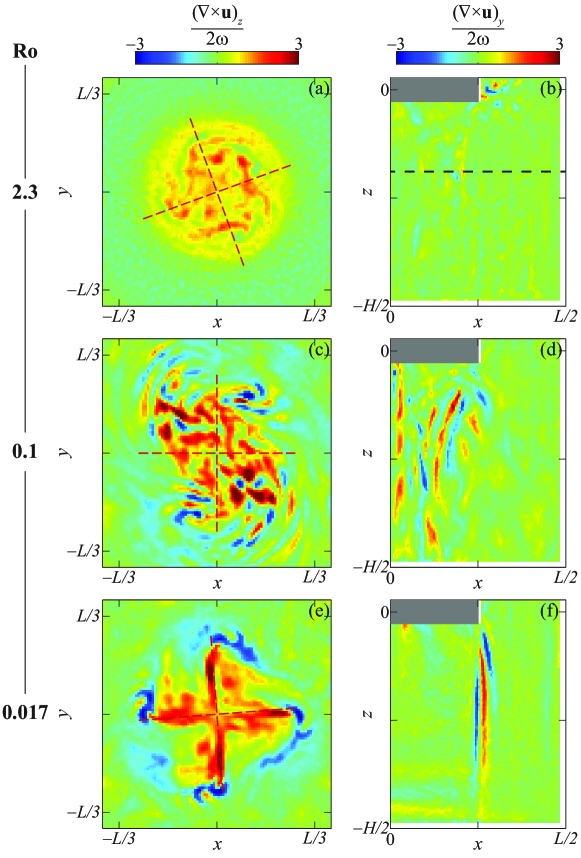
Figure 3: Vorticity fields for decreasing Rossby number ($Ro=2.3$, $0.1$ and $0.017$), revealing the small-scale features of the flow. Left column: instantaneous vertical vorticity component $(\mathbf{\nabla}\times\mathbf{u})_{z}$ at the same times than in the left column of Fig. 2. Right column: out-of-plane vorticity component $(\mathbf{\nabla}\times\mathbf{u})_{y}$ in the vertical plane $y=0$ [not at the same time than in the right column of Fig. 2 for (d) and (f)].

In addition to the large-scale geostrophic flow, we also observe small-scale three-dimensional fluctuations, mostly visible in the vorticity fields shown in Fig. 3. These vorticity fluctuations are stronger at the tip of the impeller blades for $Ro=2.3$ [Fig. 3(b)], but they are also visible in the region below the impeller [Fig. 3(a)]. As the Rossby number is decreased, vorticity sheets gradually appear below the impeller. While these vorticity sheets are disordered and fill the whole region below the impeller for $Ro=0.1$ [Figs. 3(c-d)], they become almost vertically-invariant and closely follow the shape of the impeller for $Ro=0.017$. This vertical invariance, expected in the limit of small Rossby number, is illustrated by the red cross reproducing the shape of the impeller 10 cm below it in Fig. 3(e). We further describe the dynamics of these vorticity sheets in Sec. IV.

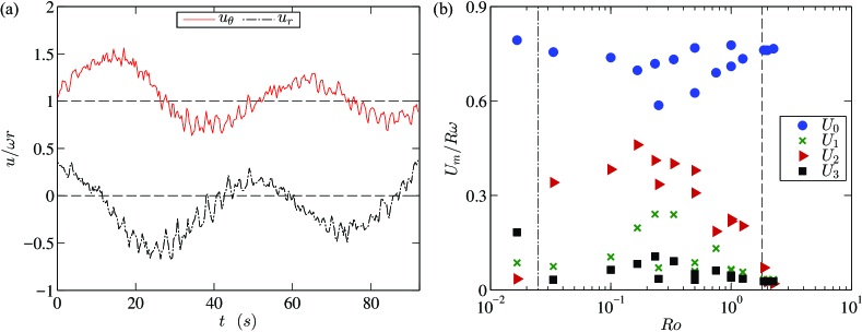
Figure 4: (a) Phase-averaged azimuthal and radial velocities, $u_{\theta}$ and $u_{r}$, as a function of time for $Ro=0.1$ at point $(x,y)=(0.4R,0)$. The main oscillation corresponds to the slow rotation of the elliptical mode $m=2$ at the angular phase velocity $\omega_{2}$. The rapid oscillations correspond to the blade crossing frequency $4\omega$. (b) Modal amplitudes $U_{m}$ of the most energetic modes $m=0-3$ as a function of the Rossby number. Vertical lines show the transition Rossby numbers $Ro_{c}^{(2-3)}$ between modes $m=2$ and 3 and $Ro_{c}^{(0-2)}$ between modes $m=0$ and 2.

For low Rossby number, the pattern of the large-scale non-axisymmetric geostrophic flow slowly rotates as a whole in the same direction as the impeller with a well-defined angular phase velocity. This is illustrated in Fig. 4(a), showing the time evolution of the azimuthal and radial velocity components at point $(x,y)=(0.4R,0)$ during one revolution of the elliptical vortex for $Ro=0.1$. The azimuthal component $u_{\theta}/\omega r$ oscillates around 1 and the radial component $u_{r}/\omega r$ oscillates around 0, both with an amplitude of order of 0.5. This indicates that, even when the axisymmetry is broken, the azimuthally averaged flow still essentially rotates at the angular velocity imposed by the impeller. The slow modulation shown in Fig. 4(a) is dominated by a mode $m=2$, but it also contains a weak mode $m=1$ (the first maximum is more pronounced than the second one), corresponding to a circular translation of the vortex axis.

We have systematically computed the modal contributions of the geostrophic flow as a function of the Rossby number. For this, we first compute for each radius $r$ and time $t$ the energy ${\cal U}^{2}_{m}(r,t)$ of the different modes $m$ from the power spectrum of the angular profile of the horizontal velocity ${\bf u}_{\perp}(r,\theta,t)$. The modal amplitude is finally obtained from a spatial (in cylindrical coordinate) and temporal average of ${\cal U}^{2}_{m}(r,t)$,

$$U_{m}=\left<\frac{4}{R^{2}}\int_{0}^{R}{\cal U}^{2}_{m}(r,t)rdr\right>^{1/2},$$ (1)

where $\langle~{}\rangle$ is the time average. Because of the non-axisymmetric boundaries of the square tank, the radial integration cannot be extended over the whole domain and is arbitrarily truncated at $r=R$. The normalization in Eq. (1) is chosen such that a solid-body rotation of angular velocity $\omega$ extending up to $r=R$ yields $U_{0}=\omega R$ and $U_{m}=0$ for $m>0$.

The amplitude $U_{m}$ of the most energetic modes $m=0-3$ are plotted in Fig. 4(b) as a function of the Rossby number. The axisymmetric contribution $m=0$ is always dominant, with a nearly constant amplitude, $U_{0}/\omega R\simeq 0.6-0.8$: these values reflect the fact that the solid-body rotation component of the flow only extends up to $r\simeq 0.7R$ (see Fig. 5 in Ref. Campagne2016 ). The amplitude of the mode $m=1$ (circular translation of the vortex core around the symmetry axis) remains moderate at all Rossby numbers, $U_{1}/\omega R\simeq 0.1-0.2$. Among the non-axisymmetric modes, the elliptical mode $m=2$ is dominant over a wide range, $Ro_{c}^{(2-3)}<Ro<Ro_{c}^{(0-2)}$, with transition Rossby numbers estimated as $Ro_{c}^{(2-3)}=0.025\pm 0.01$ and $Ro_{c}^{(0-2)}=1.75\pm 0.25$, while the triangular mode $m=3$ becomes dominant only for the smallest explored Rossby number $Ro=0.017$. Note that the data for different background rotations $\Omega$ in Fig. 4(b) suggest that the transition Rossby numbers $Ro_{c}^{(2-3)}$ and $Ro_{c}^{(0-2)}$ do not significantly depend on $\Omega$. Such critical Rossby numbers are however not expected to remain constant with $\Omega$: a weak dependence with respect to the Ekman number, $Ek=\nu/\Omega R^{2}$, is usually found in rotating-disk experiments hide_titman ; niino1984 ; fruh_read .

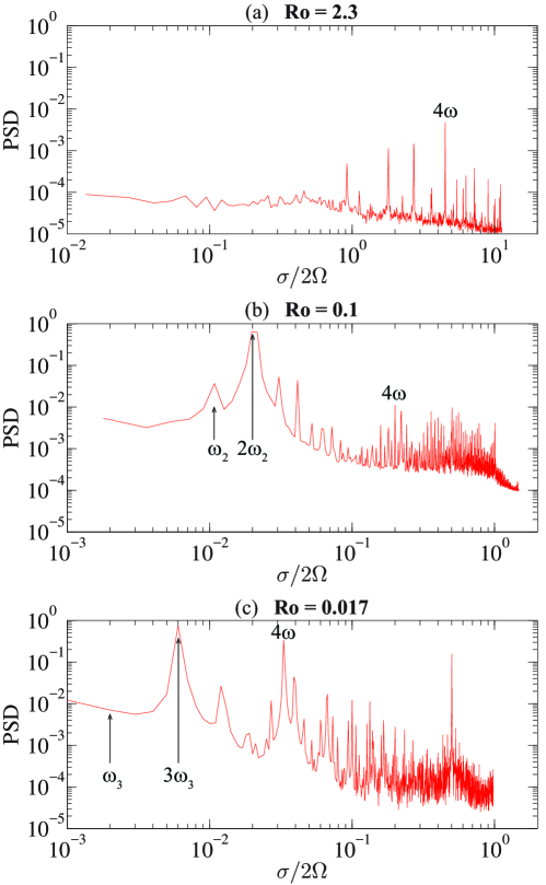
Figure 5: Temporal power spectra of the horizontal velocity field for the three Rossby numbers of Fig. 2 ($Ro=2.3$, $Ro=0.1$ and $Ro=0.017$), showing the growth of low-frequency peaks associated to the angular drift of the barotropic modes $m=2$ and $m=3$. The frequency $\sigma$ is normalized by the background vorticity $2\Omega$.

The angular phase velocity $\omega_{m}$ is further determined for each mode from a temporal Fourier analysis of the velocity measured in the horizontal plane. For all Rossby numbers, the power spectra, reported in Fig. 5, present a peak at frequency $4\omega$ corresponding to the blades motion. In addition, for $Ro<Ro_{c}^{(0-2)}$ [Figs. 5(b,c)], low-frequency peaks of larger amplitude appear: they correspond to the rotation of the non-axisymmetric geostrophic pattern. The fundamental frequency $\omega_{m}$ is only visible for $m=2$ because of the too small sampling duration for $m=3$, but its harmonic $m\omega_{m}$, which contains most of the energy, is well defined both for $m=2$ and $m=3$ [Figs. 5(b) and (c)]. The coupling of the rapid oscillations at the blade frequency $4\omega$ with the slow barotropic modulation at frequency $m\omega_{m}$ also produces a series of high-frequency harmonics at $4\omega\pm Nm\omega_{m}$, with integer $N$, surrounding the blade frequency.

The angular frequency $m\omega_{m}$ is measured for $m=2$ and $3$ from the maxima in the power spectra, and the corresponding angular phase velocity $\omega_{m}$ is reported in Fig. 6 as a function of $\omega$. We observe a linear relation, $\omega_{m}\simeq 0.2\omega$, for both $m=2$ and $3$ (note that $m=3$ is present only for the lowest Rossby number, $Ro=0.017$). This constant frequency ratio $\omega_{m}/\omega$, also observed in rotating-disk experiments hide_titman ; fruh_read , indicates that the vortex pattern, even if composed as a superposition of modes, essentially rotates as a whole. The ratio $\omega_{m}/\omega\simeq 0.2$ neither varies significantly with the background rotation $\Omega$ [see Fig. 6(b); in this plot we set $\omega_{m}=0$ for the axisymmetric mode $m=0$], here again in qualitative agreement with rotating-disk experiments.

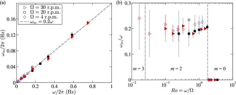
Figure 6: (a) Angular phase velocity $\omega_{m}$ of the azimuthal modes $m=2$ and 3 as a function of the impeller rotation rate $\omega$, for several platform rotation rates $\Omega$; the dashed line shows a linear fit $\omega_{m}=0.2\omega$. (b) Ratio $\omega_{m}/\omega$ versus Rossby number ($\omega_{m}$ is set to 0 for the axisymmetric mode $m=0$). Vertical lines show the transition Rossby numbers $Ro_{c}^{(2-3)}$ and $Ro_{c}^{(0-2)}$. Open (resp. filled) symbols correspond to frequency measurements in the horizontal (resp. vertical) plane. Error bars correspond to the frequency resolution of the power spectral density.

IV Wakes of Inertial waves

We now characterize the small-scale structures observed below (and above) the impeller when the azimuthal modulation of the large-scale flow is present. Figure 7(a) shows the temporal evolution of the vertical profile of the azimuthal vorticity $(\nabla\times\mathbf{u})_{y}$ at radius $r=x=0.4R$ in the case $Ro=0.1$. In this diagram the time is expressed in terms of an equivalent azimuthal coordinate $r\omega t$. We can see that almost every time a blade crosses the measurement plane (shown by vertical dashed lines) a packet of vorticity sheets of alternate sign is emitted. The thickness of the vorticity sheets along the azimuthal coordinate $r\omega t$, of order of 10 mm, is consistent with their thickness in the radial direction visible in Fig. 3(d). These vorticity packets are alternatively following and preceding the crossings of the blades, on a slow time scale given by the angular phase velocity of the geostrophic flow $m\omega_{m}$ (with $m=2$ and $\omega_{2}\simeq 0.2\omega$).

We show in the following that these packets of vorticity sheets correspond to wakes of inertial waves emitted by the blades. Such wakes originate from the azimuthal modulation of the geostrophic flow, generating a slowly evolving velocity difference

$$\Delta{\bf U}(r,\theta,t)=\omega r{\bf e}_{\theta}-{\bf u}(r,\theta,t)$$ (2)

between the blades and the fluid below and above the impeller. The radial and azimuthal components of $\Delta{\bf U}$ oscillate around 0 at frequency $m\omega_{m}$ [see Fig. 4(a)]. For instance, in the case $m=2$, when $\Delta U_{\theta}>0$, the blade is along the major axis of the ellipse and therefore rotates faster than the fluid, generating a wake behind it. On the contrary, when $\Delta U_{\theta}<0$, the blade is along the minor axis and rotates slower than the fluid, so the wake precedes the blade. In the intermediate cases, the velocity difference $\Delta{\bf U}$ is essentially radial and no clearly defined wake can be observed.

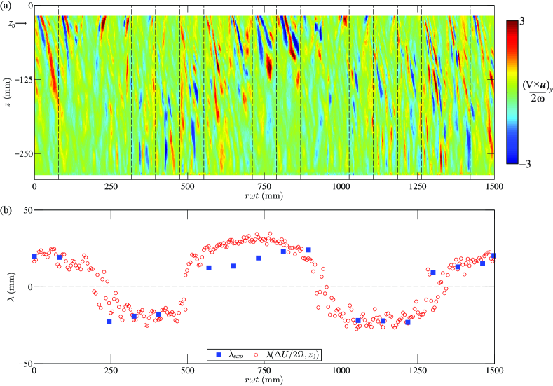
Figure 7: (a) Spatio-temporal diagram along $z$ of the azimuthal component of the vorticity $(\nabla\times\mathbf{u})_{y}$ at $Ro=0.1$, $r=x=0.4R$. The dashed lines indicate the crossings of the blades through the measurement plane. Time is expressed in terms of an effective azimuthal coordinate $r\omega t$. (b) Blue squares: horizontal wavelength in the vorticity packets induced by each blade crossing the measurement plane, measured at height $z_{0}=-30$ mm. This wavelength is computed from the vorticity autocorrelation over a window along the coordinate $r\omega t$, and its sign is set to negative when the wake precedes the blade. Red circles: predicted wavelength from Eq. (3), computed using the instantaneous azimuthal velocity difference between the fluid and the blade $\Delta U_{\theta}$.

In order to confirm this picture, we can refer to the simple model of a linear inviscid wake of inertial waves produced by the translation of a source, analyzed by Lighthill Lighthill1967 and Peat & Stevenson peat1976 . We consider a line source, invariant along $Y$, traveling at constant velocity $U$ in the direction $X>0$ normal to the rotation axis $Z$. In the frame of the source, the phase field $\varphi(X,Z)$ of the wake is such that the lines of constant phase $\varphi$ write

$$\begin{cases}X=-\lambda_{0}\dfrac{\varphi}{2\pi}\dfrac{2-\cos^{2}\theta}{\cos\theta},\\ Z=\lambda_{0}\dfrac{\varphi}{2\pi}\dfrac{\sin^{3}\theta}{\cos^{2}\theta},\end{cases}$$ (3)

where

$$\lambda_{0}=\pi U/\Omega$$ (4)

is the natural wavelength along the source trajectory, and $\theta$ a parameter ranging from $0$ to $\pi/2$. The wave field $\cos\varphi$ is shown in Fig. 8 in normalized coordinates $(X,Z)/\lambda_{0}$. The wavelength $\lambda_{0}$ is $2\pi$ times the gyration radius $U/2\Omega$ of a fluid particle oscillating horizontally at velocity $U$ and natural frequency $2\Omega$ in the inertial wave.

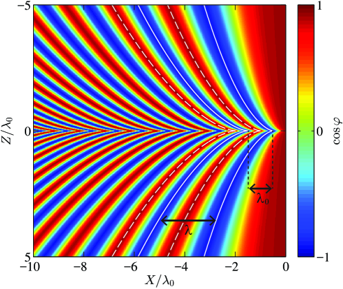
Figure 8: Phase field $\cos\varphi$ (3) of the linear inviscid wake of inertial waves produced by the translation of a line source in the direction $X>0$ at a constant velocity $U$. The axis are normalized by the natural wavelength $\lambda_{0}$ (4) along the wake axis. White lines show lines of constant phase $\varphi=\pi$, $2\pi$, $3\pi$, and $4\pi$ from right to left.

In order to compare the shape of the wave packets observed in Fig. 7(a) to the phase lines of this simplified model, we approximate the blade motion locally as a linear translation (we therefore neglect the curvature of the trajectory), so that we can identify in Eqs. (3)-(4) the source velocity $U$ to the (slowly varying in time) azimuthal component $\Delta U_{\theta}$ of the velocity difference between the blade and the fluid, and the coordinate $X$ to the equivalent azimuthal coordinate $r\omega t$.

For each wave beam, we first compute the characteristic wavelength $\lambda_{exp}$ at a fixed distance $z_{0}=-30$ mm below the impeller. We define $\lambda_{exp}$ as twice the scale corresponding to the first minimum of the vorticity autocorrelation function computed over a window of 80 mm along $X=r\omega t$ and centered on the wave beam of interest. We set the sign of $\lambda_{exp}$ as positive when the wake follows the blade and negative when it precedes it. This characteristic wavelength is plotted in Fig. 7(b), and compared with the predicted wavelength from Eq. (3), evaluated for the same value of $Z$ and for the azimuthal component $\Delta U_{\theta}$ of the velocity difference $\Delta{\bf U}$ at the same time. In spite of the simplicity of the model, we obtain a reasonable agreement between the measured and the predicted wavelength. The discrepancies can be ascribed to the various assumptions of the model which are not satisfied in the experiment: in addition to the curvature of the source trajectory, the model neglects the finite size of the source, the radial component of the velocity difference $\Delta{\bf U}$, and the variation with time of $\Delta U_{\theta}$.

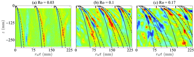
Figure 9: Spatio-temporal diagrams of the azimuthal component of the vorticity along $z$ at $(x,y)=(0.4R,0)$ for three Rossby numbers. Black lines show lines of constant phase $\varphi=\pi$, $2\pi$, $3\pi$, and $4\pi$ (from left to right) given by Eq. (3). For each wake, the origin $(X=0,Z=0)$ of the reference frame of the phase lines in Eq. (3) is taken at the center of the blade, at the time given by the blade crossing the measurement plane. The value of $\lambda_{0}$ in Eq. (3) is computed from the instantaneous azimuthal velocity difference $\Delta U_{\theta}$ between the fluid and the blade.

We further test our description by superposing the predicted phase lines (3) on the spatio-temporal diagrams in Fig. 9 for three values of the Rossby number, $Ro=0.03$, $0.1$ and $0.17$, for which the dominant mode is $m=2$. Three blade crossings are shown for each $Ro$, chosen during time intervals for which $\Delta U_{\theta}$ is positive (i.e., when the wakes follow the blades) and approximately constant. Here again a reasonable match is obtained, at least for $Ro=0.03$ and 0.1, which confirms that the small-scale fluctuations at low $Ro$ correspond to wakes of inertial waves emitted by the blades. As expected the vorticity field becomes increasingly disordered as $Ro$ increases, as the result of instabilities in the wakes or interactions of the wakes with the turbulent structures directly produced by the blade motion, and the match with the model (3) becomes worse as $Ro$ approaches $O(1)$.

V Conclusion

We have characterized in this paper the two-dimensionalization process in the flow produced by a slowly rotating impeller in a rapidly rotating fluid, extending the range of Rossby numbers of Campagne et al. Campagne2016 down to $10^{-2}$. Although two-dimensionality is already satisfied for the mean flow at $Ro\simeq O(1)$, the small scales remain three-dimensional and disordered down to $10^{-2}$. In this regime the flow can be described as the superimposition of a large-scale azimuthally modulated geostrophic flow and small-scale vorticity sheets, which correspond to wakes of inertial waves originating from the velocity difference between the impeller and the non-axisymmetric geostrophic flow. This situation is expected in general for flows produced by a non-axisymmetric rotating device, in contrast to experiments with axisymmetric forcing, as in Hide & Titman hide_titman .

We expect that this regime of disordered wakes at Rossby number $Ro\simeq 10^{-2}-1$ is a transient in the route towards pure two-dimensionalization: as the Rossby number is further decreased, the barotropic instability should lead to azimuthal modulations of increasing order $m$, associated with a decreasing velocity difference between the geostrophic flow and the impeller. In this limit the wakes produced by the blades should become vertical, a tendency already visible in Fig. 3(f), protruding the shape of the impeller to $z\rightarrow\pm\infty$, eventually leading to a pure two-dimensional flow at vanishing Rossby number. Interestingly, the disordered wake regime observed here may form, at larger Reynolds number, a particular state of inertial wave turbulence Galtier2003 ; Cambon2004 ; Nazarenko : the localized wave generation implies an upward and downward energy propagation on each side of the impeller, leading to a separation of the sign of helicity Ranjan2014 .

References

- (1) H. Greenspan, The Theory of Rotating Fluids (Cambridge University Press, Cambridge, UK, 1968).
- (2) P. A. Davidson, Turbulence in rotating, stratified and electrically conducting fluids (Cambridge University Press, Cambridge, 2013).
- (3) F. S. Godeferd and F. Moisy, Structure and dynamics of rotating turbulence: a review of recent experimental and numerical results, Applied Mechanics Reviews 67, 030802 (2015).
- (4) P. Clark di Leoni, P. J. Cobelli, P. D. Mininni, P. Dmitruk, and W. H. Matthaeus, Quantification of the strength of inertial waves in a rotating turbulent flow, Phys. Fluids 26, 035106 (2014).
- (5) E. Yarom and A. Sharon, Experimental observation of steady inertial wave turbulence in deep rotating flows, Nature Physics 10, 510 (2014).
- (6) A. Campagne, B. Gallet, F. Moisy, P.-P. Cortet, Disentangling inertial waves from eddy turbulence in a forced rotating-turbulence experiment, Phys. Rev. E 91, 043016 (2015).
- (7) A. D. McEwan, Inertial oscillations in a rotating fluid cylinder. J Fluid Mech 40, 603 (1970).
- (8) N. Machicoane, P.-P. Cortet, B. Voisin, and F. Moisy, Influence of the multipole order of the source on the decay of an inertial wave beam in a rotating fluid, Phys. Fluids 27, 066602 (2015)
- (9) B. Gallet, Exact two-dimensionalization of rapidly rotating large-Reynolds-number flows, J. Fluid Mech. 783, 412 (2015).
- (10) J. Pedlosky, Geophysical Fluid Dynamics (Springer-Verlag, New York, USA, 1987).
- (11) G. K. Vallis, Atmospheric and Oceanic Fluid Dynamics: Fundamentals and Large-scale circulation (Cambridge University Press, UK, 2006).
- (12) Y. B. Baqui and P. A. Davidson, A phenomenological theory of rotating turbulence, J. Fluid Mech. 27, 025107 (2015).
- (13) A. Campagne, B. Gallet, F. Moisy and P.-P. Cortet, Direct and inverse energy cascades in a forced rotating turbulence experiment, Phys. Fluids 26, 125112 (2014).
- (14) E. Yarom, Y. Vardi, and A. Sharon, Experimental quantification of inverse energy cascade in deep rotating turbulence, Phys. Fluids 25, 085105 (2013).
- (15) L. Bourouiba, D. N. Straub, and M. L. Waite, Non-local energy transfers in rotating turbulence at intermediate Rossby number, J. Fluid Mech. 690, 129 (2012).
- (16) T. Teitelbaum and P. D. Mininni, Decay of Batchelor and Saffman Rotating Turbulence, Phys. Rev. E 86, 066320 (2012).
- (17) E. Deusebio, G. Boffetta, E. Lindborg, S. Musacchio, Dimensional transition in rotating turbulence, Phys. Rev. E 90, 023005 (2014).
- (18) A. Delache, C. Cambon, and F. S. Godeferd, Scale by scale anisotropy in freely decaying rotating turbulence, Phys. Fluids 26, 025104 (2014).
- (19) A. Alexakis, Rotating Taylor-Green flow, J. Fluid Mech. 769, 46 (2015).
- (20) A. Campagne, N. Machicoane, B. Gallet, P.-P. Cortet, and F. Moisy, Turbulent drag in a rotating frame, J. Fluid Mech. 794, R5 (2016).
- (21) R. Hide, and C. W. Titman, Detached shear layers in a rotating fluid, J. Fluid Mech. 29, 39 (1967).
- (22) K. Stewartson, On almost rigid rotations, J. Fluid Mech. 3, 17 (1957).
- (23) F. H. Busse, Shear flow instabilities in rotating systems, J. Fluid Mech. 33, 577 (1968).
- (24) H. Niino, and N. Misawa, An experimental and theoretical study of barotropic instability, J. Atmos. Sc. 41, 1992 (1984).
- (25) F. V. Dolzhanskii, V. A. Krymov, D. Yu Manin, Stability and vortex structures of quasi-two-dimensional shear flows, Sov. Phys. Usp 33 (7), 495 (1990).
- (26) J. A. van de Konijnenberg, A. H. Nielsen, J. J. Rasmussen, and B. Stenum, Shear-flow instability in a rotating fluid, J. Fluid Mech. 387, 177 (1999).
- (27) W. G. Früh and P. L. Read, Experiments on a barotropic rotating shear layer. Part 1. Instability and steady vortices, J. Fluid Mech. 383, 143 (1999).
- (28) R. Hollerbach, Instabilities of the Stewartson layer. Part 1. The dependence on the sign of , J. Fluid Mech. 492, 289 (2003).
- (29) N. Schaeffer and P. Cardin, Quasigeostrophic Model of the Instabilities of the Stewartson Layer in Flat and Depth-Varying Containers, Phys. Fluids 17, 104111 (2005).
- (30) M. J. Lighthill, On waves generated in dispersive systems to traveling forcing effects, with applications to the dynamics of rotating fluids, J. Fluid Mech. 27, 725 (1967).
- (31) K. S. Peat and T. N. Stevenson, The phase configuration of waves around a body moving in a rotating stratified fluid, J. Fluid Mech. 75, 647 (1976).
- (32) S. Galtier, Weak inertial-wave turbulence theory, Phys. Rev. E 68, 015301 (2003).
- (33) C. Cambon, R. Rubinstein, and F. S. Godeferd, Advances in wave turbulence: rapidly rotating flows, New J. Phys. 6, 73 (2004).
- (34) S. Nazarenko, Wave Turbulence (Springer-Verlag, 2011).
- (35) A. Ranjan and P. A. Davidson, Evolution of a turbulent cloud under rotation, J. Fluid Mech. 756, 488 (2014).