Designing Sparse Reliable Pose-Graph SLAM:
A Graph-Theoretic Approach

Abstract

In this paper, we aim to design sparse D-optimal (determinant-optimal) pose-graph SLAM problems through the synthesis of sparse graphs with the maximum weighted number of spanning trees. Characterizing graphs with the maximum number of spanning trees is an open problem in general. To tackle this problem, several new theoretical results are established in this paper, including the monotone log-submodularity of the weighted number of spanning trees. By exploiting these structures, we design a complementary pair of near-optimal efficient approximation algorithms with provable guarantees. Our theoretical results are validated using random graphs and a publicly available pose-graph SLAM dataset.

1 Introduction

Graphs arise in modelling numerous phenomena across science and engineering. In particular, estimation-on-graph (EoG) is a class of (maximum likelihood) estimation problems with a natural graphical representation that arise especially in robotics and sensor networks. In such problems, each vertex corresponds to an unknown state, and each edge corresponds to a relative noisy measurement between the corresponding states. Simultaneous localization and mapping (SLAM) and sensor network localization (SNL) are two well-studied EoGs.

Designing sparse, yet “well-connected” graphs is a subtle task that frequently arises in various domains. First, note that graph sparsity—in EoGs and many other contexts—lead to computational efficiency. Hence, maintaining sparsity is often crucial. It is useful to see graph connectivity as a spectrum, as we often need to compare the connectivity of connected graphs. In engineering, well-connected graphs often exhibit desirable qualities such as reliability, robustness, and resilience to noise, outliers, and link failures. More specifically, a well-connected EoG is more resilient to a fixed noise level and results in a more reliable estimate (i.e., smaller estimation-error covariance in the Loewner ordering sense). Consequently, maintaining a sufficient connectivity is also critical. Needless to say, sparsity is, by its very essence, at odds with well-connectivity. This is the case in SLAM, where there is a trade-off between the cost of inference and the reliability of the resulting estimate. This problem is not new. Measurement selection and pose-graph pruning have been extensively studied in the SLAM literature (see, e.g., [21, 12]). However, in this paper we take a novel graph-theoretic approach by reducing the problem of designing sparse reliable SLAM problems to the purely combinatorial problem of synthesizing sparse, yet well-connected graphs. In what follows, we briefly justify this approximate reduction.

First, note that by estimation reliability we refer to the standard D-optimality criterion, defined as the determinant of the (asymptotic) maximum likelihood estimator covariance matrix. D-optimality is a standard and popular design criterion; see, e.g., [13, 16] and the references therein. Next, we have to specify how we measure graph connectivity. Among the existing combinatorial and spectral graph connectivity criteria, the number of spanning trees (sometimes referred to as graph complexity or tree-connectivity) stands out: despite its combinatorial origin, it can also be characterized solely by the spectrum of the graph Laplacian [9]. In [16, 17, 18], we shed light on the connection between the D-criterion in SLAM—and some other EoGs—and the tree-connectivity of the underlying graph. Our theoretical and empirical results demonstrate that, under some standard conditions, D-optimality in SLAM is significantly influenced by the tree-connectivity of the graph underneath. Therefore, one can accurately estimate the D-criterion without using any information about the robot’s trajectory or realized measurements (see Section 3). Intuitively speaking, our approach can be seen as a dimensionality reduction scheme for designing D-optimal SLAM problems from the joint space of trajectories and graph topologies to only the space of graph topologies [18].

Although this work is specifically motivated by the SLAM problem, designing sparse graphs with the maximum tree-connectivity has several other important applications. For example, it has been shown that tree-connectivity is associated with the D-optimal incomplete block designs [7, 5, 1]. Moreover, tree-connectivity is a major factor in maximizing the connectivity of certain random graphs that model unreliable networks under random link failure (all-terminal network reliability) [15, 30]. In particular, a classic result in network reliability theory states that if the uniformly-most reliable network exits, it must have the maximum tree-connectivity among all graphs with the same size [2, 23, 3].

Known Results.

Graphs with the maximum weighted number of spanning trees among a family of graphs with the same vertex set are called $t$-optimal. The problem of characterizing unweighted $t$-optimal graphs among the set of graphs with $n$ vertices and $m$ edges remains open and has been solved only for specific pairs of $n$ and $m$; see, e.g., [27, 5, 14, 25]. The span of these special cases is too narrow for the types of graphs that typically arise in SLAM and sensor networks. Furthermore, in many cases the $(n,m)$ constraint alone is insufficient for describing the true set of “feasible” graphs and cannot capture implicit practical constraints that exist in SLAM. Finally, it is not clear how these results can be extended to the case of (edge) weighted graphs, which are essential for representing SLAM problems, where the weight of each edge represents the precision of the corresponding pairwise measurement [18].

Contributions.

This paper addresses the problem of designing sparse $t$-optimal graphs with the ultimate goal of designing D-optimal pose-graph SLAM problems. First and foremost, we formulate a combinatorial optimization problem that captures the measurement selection and measurement pruning scenarios in SLAM. Next, we prove that the weighted number of spanning trees, under certain conditions, is a monotone log-submodular function of the edge set. To the best of our knowledge, this is a new result in graph theory. Using this result, we prove that the greedy algorithm is near-optimal. In our second approximation algorithm, we formulate this problem as an integer program that admits a straightforward convex relaxation. Our analysis sheds light on the performance of a simple deterministic rounding procedure that have also been used in more general contexts. The proposed approximation algorithms provide near-optimality certificates. The proposed graph synthesis framework can be readily applied to any application where maximizing tree-connectivity is desired.

Notation.

Throughout this paper, bold lower-case and upper-case letters are reserved for vectors and matrices, respectively. The standard basis for $\mathbb{R}^{n}$ is denoted by $\{\mathbf{e}_{i}^{n}\}_{i=1}^{n}$. Sets are shown by upper-case letters. $|\cdot|$ denotes the set cardinality. For any finite set $\mathcal{W}$, $\binom{\mathcal{W}}{k}$ is the set of all $k$-subsets of $\mathcal{W}$. We use $[n]$ to denote the set $\{1,2,\dots,n\}$. The eigenvalues of symmetric matrix $\mathbf{M}$ are denoted by $\lambda_{1}(\mathbf{M})\leq\dots\leq\lambda_{n}(\mathbf{M})$. $\mathbf{1}$, $\mathbf{I}$ and $\mathbf{0}$ denote the vector of all ones, the identity and the zero matrices with appropriate sizes, respectively. $\mathbf{S}_{1}\succ\mathbf{S}_{2}$ (resp. $\mathbf{S}_{1}\succeq\mathbf{S}_{2}$) means $\mathbf{S}_{1}-\mathbf{S}_{2}$ is positive definite (resp. positive semidefinite). Finally, $\mathop{\mathrm{diag}}(\mathbf{W}_{1},\dots,\mathbf{W}_{k})$ is the block-diagonal matrix whose main diagonal blocks are $\mathbf{W}_{1},\dots,\mathbf{W}_{k}$.

2 Preliminaries

Graph Matrices.

Throughout this paper, we usually refer to undirected graphs $\mathcal{G}=(\mathcal{V},{\mathcal{E}})$ with $n$ vertices (labeled with $[n]$) and $m$ edges. With a little abuse of notation, we call $\widetilde{\mathbf{A}}\in\{-1,0,1\}^{n\times m}$ the incidence matrix of $\mathcal{G}$ after choosing an arbitrary orientation for its edges. The Laplacian matrix of $\mathcal{G}$ is defined as $\widetilde{\mathbf{L}}\triangleq\widetilde{\mathbf{A}}\widetilde{\mathbf{A}}^{\top}$. $\widetilde{\mathbf{L}}$ can be written as $\sum_{i=1}^{m}\widetilde{\mathbf{L}}_{e_{i}}$ in which $\widetilde{\mathbf{L}}_{e_{i}}$ is the elementary Laplacian associated with edge $e_{i}=\{u_{i},v_{i}\}$, where the $(u_{i},u_{i})$ and $(v_{i},v_{i})$ entries are $1$, and the $(u_{i},v_{i})$ and $(v_{i},u_{i})$ entries are $-1$. Anchoring $v_{0}\in\mathcal{V}$ is equivalent to removing the row associated with $v_{0}$ from $\widetilde{\mathbf{A}}$. Anchoring $v_{0}$ results in the reduced incidence matrix $\mathbf{A}$ and the reduced Laplacian matrix $\mathbf{L}\triangleq\mathbf{A}\mathbf{A}^{\top}$. $\mathbf{L}$ is also known as the Dirichlet. We may assign positive weights to the edges of $\mathcal{G}$ via $w:{\mathcal{E}}\to\mathbb{R}_{>0}$. Let $\mathbf{W}\in\mathbb{R}^{m\times m}$ be the diagonal matrix whose $(i,i)$ entry is equal to the weight of the $i$th edge. The weighted Laplacian (resp. reduced weighted Laplacian) is then defined as $\widetilde{\mathbf{L}}_{w}\triangleq\widetilde{\mathbf{A}}\mathbf{W}\widetilde{\mathbf{A}}^{\top}$ (resp. $\mathbf{L}_{w}\triangleq\mathbf{A}\mathbf{W}\mathbf{A}^{\top}$). Note that the (reduced) unweighted Laplacian is a special case of the (reduced) weighted Laplacian with $\mathbf{W}=\mathbf{I}_{m}$ (i.e., when all edges have unit weight).

Spanning Trees.

A spanning tree of ${\mathcal{G}}$ is a spanning subgraph of ${\mathcal{G}}$ that is also a tree. Let $\mathbb{T}_{\mathcal{G}}$ denote the set of all spanning trees of $\mathcal{G}$. $t(\mathcal{G})\triangleq|\mathbb{T}_{\mathcal{G}}|$ denotes the number of spanning trees in $\mathcal{G}$. As a generalization, for graphs whose edges are weighted by $w:{\mathcal{E}}\to\mathbb{R}_{>0}$, we define the weighted number of spanning trees,

$$t_{w}(\mathcal{G})\triangleq\sum_{\mathcal{T}\in\mathbb{T}_{\mathcal{G}}}\mathbb{V}_{w}(\mathcal{T}).$$ (1)

We call $\mathbb{V}_{w}:\mathbb{T}_{\mathcal{G}}\to\mathbb{R}_{>0}$ the tree value function and define it as the product of the edge weights along a spanning tree. Notice that for unit edge weights, $t_{w}(\mathcal{G})$ coincides with $t(\mathcal{G})$. Thus, unless explicitly stated otherwise, we generally assume the graph is weighted. To prevent overflow and underflow, it is more convenient to work with $\log t_{w}(\mathcal{G})$. We formally define tree-connectivity as,

$$\tau_{w}(\mathcal{G})\triangleq\begin{cases}\log t_{w}(\mathcal{G})&\text{if $\mathcal{G}$ is connected,}\\ 0&\text{otherwise.}\end{cases}$$ (2)

For the purpose of this work, without loss of generality we can assume $w(e)\geq 1$ for all $e\in{\mathcal{E}}$, and thus $\tau_{w}(\mathcal{G})\geq 0$. The equality occurs only when either $\mathcal{G}$ is not connected, or when $\mathcal{G}$ is a tree whose all edges have unit weight. Kirchhoff’s seminal matrix-tree theorem is a classic result in spectral graph theory. This theorem relates the spectrum of the Laplacian matrix of graph to its number of spanning trees. The original matrix-tree theorem states that,

$$t(\mathcal{G}) =\det\mathbf{L}$$ (3)

$$=\frac{1}{n}\prod_{i=2}^{n}\lambda_{i}(\widetilde{\mathbf{L}}).$$ (4)

Here $\mathbf{L}$ is the reduced Laplacian after anchoring an arbitrary vertex. Kirchhoff’s matrix-tree theorem has been generalized to the case of edge-weighted graphs. According to the generalized theorem, $t_{w}(\mathcal{G})=\det\mathbf{L}_{w}=\frac{1}{n}\prod_{i=2}^{n}\lambda_{i}(\widetilde{\mathbf{L}}_{w})$.

Submodularity.

Suppose $\mathcal{W}$ is a finite set. Consider a set function $\xi:2^{\mathcal{W}}\to\mathbb{R}$. $\xi$ is called:

1. normalized  iff $\xi(\varnothing)=0$.

2. monotone     iff $\xi(\mathcal{B})\geq\xi(\mathcal{A})$ for every $\mathcal{A}$ and $\mathcal{B}$ s.t. $\mathcal{A}\subseteq\mathcal{B}\subseteq\mathcal{W}$.

3. submodular iff for every $\mathcal{A}$ and $\mathcal{B}$ s.t. $\mathcal{A}\subseteq\mathcal{B}\subseteq\mathcal{W}$ and $\forall s\in\mathcal{W}\setminus\mathcal{B}$ we have,

   $$\xi(\mathcal{A}\cup\{s\})-\xi(\mathcal{A})\geq\xi(\mathcal{B}\cup\{s\})-\xi(\mathcal{B}).$$ (5)

3 D-Optimality via Graph Synthesis

In this section, we discuss the connection between D-optimality and $t$-optimality in SLAM by briefly reviewing the results in [16, 17, 18]. Consider the 2-D pose-graph SLAM problem where each measurement consists of the rotation (angle) and translation between a pair of robot poses over time, corrupted by an independently-drawn additive zero-mean Gaussian noise. According to our model, the covariance matrix of the noise vector corrupting the $i$th measurement can be written as $\mathop{\mathrm{diag}}(\sigma_{p_{i}}^{2}\mathbf{I}_{2},\sigma_{\theta_{i}}^{2})$, where $\sigma_{p_{i}}^{2}$ and $\sigma_{\theta_{i}}^{2}$ denote the translational and rotational noise variances, respectively. As mentioned earlier, SLAM, as an EoG problem, admits a natural graphical representation $\mathcal{G}=(\mathcal{V},{\mathcal{E}})$ in which poses correspond to graph vertices and edges correspond to the relative measurements between the corresponding poses. Furthermore, measurement precisions are incorporated into our model by assigning positive weights to the edges of $\mathcal{G}$. Note that for each edge we have two separate weight functions $w_{p}$ and $w_{\theta}$, defined as $w_{p}:e_{i}\mapsto\sigma_{p_{i}}^{-2}$ and $w_{\theta}:e_{i}\mapsto\sigma_{\theta_{i}}^{-2}$.

Let $\mathbb{V}\mathrm{ar}[\hat{\mathbf{x}}_{\textsf{mle}}]$ be the asymptotic covariance matrix of the maximum likelihood estimator (Cramér-Rao lower bound) for estimating the trajectory $\mathbf{x}$. In [16, 17, 18], we investigated the impact of graph topology on the D-optimality criterion ($\det\mathbb{V}\mathrm{ar}[\hat{\mathbf{x}}_{\textsf{mle}}]$) in SLAM. The results presented in [18] are threefold. First, in [18, Proposition 2] it is proved that

$$-2\,\tau_{w_{p}}(\mathcal{G})-\log\det(\mathbf{L}_{w_{\theta}}+\gamma\mathbf{I})\leq\log\det\mathbb{V}\mathrm{ar}[\hat{\mathbf{x}}_{\textsf{mle}}]\leq-2\,\tau_{w_{p}}(\mathcal{G})-\tau_{w_{\theta}}(\mathcal{G})\vspace{-3pt}$$ (6)

in which $\gamma$ is a parameter whose value depends on the maximum distance between the neighbouring robot poses normalized by $\sigma_{p_{i}}^{2}$’s; e.g., this parameter shrinks by reducing the distance between the neighbouring poses, or by reducing the precision of the translational measurements (see [18, Remark 2]). Next, based on this result, it is easy to see that [18, Theorem 5],

$$\lim_{\gamma\to 0^{+}}\log\det\mathbb{V}\mathrm{ar}[\hat{\mathbf{x}}_{\textsf{mle}}]=-2\,\tau_{w_{p}}(\mathcal{G})-\tau_{w_{\theta}}(\mathcal{G}).\vspace{-3pt}$$ (7)

Note that the expression above depends only on the graphical representation of the problem. Finally, the empirical observations and Monte Carlo simulations based on a number of synthetic and real datasets indicate that the RHS of (7) provides a reasonable estimate for $\log\det\mathbb{V}\mathrm{ar}[\hat{\mathbf{x}}_{\textsf{mle}}]$ even in the non-asymptotic regime where $\gamma$ is not negligible. In what follows, we demonstrate how these results can be used in a graph-theoretic approach to the D-optimal measurement selection and pruning problems.

Measurement Selection.

Maintaining sparsity is essential for computational efficiency in SLAM, especially in long-term autonomy. Sparsity can be preserved by implementing a measurement selection policy to asses the significance of new or existing measurements. Such a vetting process can be realized by (i) assessing the significance of any new measurement before adding it to the graph, and/or (ii) pruning a subset of the acquired measurements if their contribution is deemed to be insufficient. These ideas have been investigated in the literature; for the former approach see, e.g., [13, 26], and see, e.g., [21, 12] for the latter.

Now consider the D-optimal measurement selection problem whose goal is to select the optimal $k$-subset of measurements such that the resulting $\log\det\mathbb{V}\mathrm{ar}[\hat{\mathbf{x}}_{\textsf{mle}}]$ is minimized. This problem is closely related to the D-optimal sensor selection problem for which two successful approximation algorithms have been proposed in [13] and [26] under the assumption of linear sensor models. The measurement models in SLAM are nonlinear. Nevertheless, we can still use [13, 26] after linearizing the measurement model. Note that the Fisher information matrix and $\log\det\mathbb{V}\mathrm{ar}[\hat{\mathbf{x}}_{\textsf{mle}}]$ in SLAM depend on the true $\mathbf{x}$. Since the true value of $\mathbf{x}$ is not available, in practice these terms are approximated by evaluating the Jacobian matrix at the estimate obtained by maximizing the log-likelihood function using an iterative solver.

An alternative approach would be to replace $\log\det\mathbb{V}\mathrm{ar}[\hat{\mathbf{x}}_{\textsf{mle}}]$ with a graph-theoretic objective function based on (7). Note that this is equivalent to reducing the original problem into a graph synthesis problem. The graphical approach has the following advantages:

1. Robustness: Maximum likelihood estimation in SLAM boils down to solving a non-convex optimization problem via iterative solvers. These solvers are subject to local minima. Hence, the approximated $\log\det\mathbb{V}\mathrm{ar}[\hat{\mathbf{x}}_{\textsf{mle}}]$ can be highly inaccurate and lead to misleading designs if the Jacobian is evaluated at a local minimum (see [18, Section VI] for an example). The graph-theoretic objective function based on (7), however, is independent of the trajectory $\mathbf{x}$ and, therefore, is robust to such convergence errors.

2. Flexibility: To directly compute $\log\det\mathbb{V}\mathrm{ar}[\hat{\mathbf{x}}_{\textsf{mle}}]$, we first need a nominal or estimated trajectory $\mathbf{x}$. Furthermore, for the latter we also need to know the realization of relative measurements. Therefore, any design or decisions made in this way will be confined to a particular trajectory. On the contrary, the graphical approach requires only the knowledge of the topology of the graph, and thus is more flexible. Note that the $t$-optimal topology corresponds to a range of trajectories. Therefore, the graphical approach enables us to assess the D-optimality of a particular design with minimum information and without relying on any particular—planned, nominal or estimated—trajectory.

We will investigate the problem of designing $t$-optimal graphs in Section 4.

4 Synthesis of Near-$t$-Optimal Graphs

Problem Formulation.

In this section, we formulate and tackle the combinatorial optimization problem of designing sparse graphs with the maximum weighted tree-connectivity. Since the decision variables are the edges of the graph, it is more convenient to treat the weighted tree-connectivity as a function of the edge set of the graph for a given set of vertices ($\mathcal{V}=[n]$) and a positive weight function $w:\binom{[n]}{2}\to\mathbb{R}_{\geq 1}$. $\mathsf{tree}_{n,w}:2^{\binom{[n]}{2}}\to\mathbb{R}_{\geq 0}:{\mathcal{E}}\mapsto\tau_{w}([n],{\mathcal{E}})$ takes as input a set of edges ${\mathcal{E}}$ and returns the weighted tree-connectivity of graph $([n],{\mathcal{E}})$. To simplify our notation, hereafter we drop $n$ and/or $w$ from $\mathsf{tree}_{n,w}$ (and similar terms) whenever $n$ and/or $w$ are clear from the context.

Remark 1

It is easy to see that any instance of (8) can be expressed as an instance of (9) and vice versa. Therefore, without loss of generality, in this work we only consider $k$-$\mathrm{ESP}^{\texttt{+}}$.

$1$-$\mathrm{ESP}^{\texttt{+}}$.

Consider the simple case of $k=1$. $\Delta_{uv}\triangleq\mathbf{a}_{uv}\mathbf{L}^{-1}\mathbf{a}_{uv}$ is known as the effective resistance between vertices $u$ and $v$. Here $\mathbf{a}_{uv}\in\{-1,0,1\}^{n-1}$ is the vector $\mathbf{e}_{u}^{n}-\mathbf{e}_{v}^{n}$ after crossing out the entry that corresponds to the anchored vertex. Effective resistance has emerged from several other contexts as a key factor; see, e.g., [8]. In [19, Lemma 3.1] it is shown that the optimal choice in $1$-$\mathrm{ESP}^{\texttt{+}}$ is the candidate edge with the maximum $w(e)\Delta_{e}$. The effective resistance can be efficiently computed by performing a Cholesky decomposition on the reduced weighted Laplacian matrix of the base graph ${\mathbf{L}}_{\text{init}}$ and solving a triangular linear system (see [19]). In the worst case and for a dense base graph $1$-$\mathrm{ESP}^{\texttt{+}}$ can be solved in $O(n^{3}+c\,n^{2})$ time.

4.1 Approximation Algorithms for $k$-$\mathrm{ESP}^{\texttt{+}}$

Solving the general case of $k$-$\mathrm{ESP}^{\texttt{+}}$ by exhaustive search requires examining $\binom{c}{k}$ graphs. This is not practical even when $c$ is bounded (e.g., for $c=30$ and $k=10$ we need to perform more than $3\times 10^{7}$ Cholesky factorizations). Here we propose a complementary pair of approximation algorithms.

4.1.1 I: Greedy.

The greedy algorithm finds an approximate solution to $k$-$\mathrm{ESP}^{\texttt{+}}$ by decomposing it into a sequence of $k$ $1$-$\mathrm{ESP}^{\texttt{+}}$ problems, each of which can be solved using the procedure outlined above. After solving each subproblem, the optimal edge is moved from the candidate set to the base graph. The next $1$-$\mathrm{ESP}^{\texttt{+}}$ subproblem is defined using the updated candidate set and the updated base graph. If the graph is dense, a naive implementation of the greedy algorithm requires less than $O(kcn^{3})$ operations. An efficient implementation of this approach that requires $O(n^{3}+kcn^{2})$ time is described in [19, Algorithm 1].

Analysis.

Let ${\mathcal{G}}_{\text{init}}=([n],{{{\mathcal{E}}}_{\text{init}}})$ be a connected base graph and $w:\binom{[n]}{2}\to\mathbb{R}_{\geq 1}$. Consider the following function.

$$\mathcal{X}_{w}:{\mathcal{E}}\mapsto\mathsf{tree}({{\mathcal{E}}\cup{{{\mathcal{E}}}_{\text{init}}}})-\mathsf{tree}({{{{\mathcal{E}}}_{\text{init}}}}).$$ (10)

In $k$-$\mathrm{ESP}^{\texttt{+}}$, we restrict the domain of $\mathcal{X}_{w}$ to $2^{\mathcal{C}^{\texttt{+}}}$. Note that $\mathsf{tree}({{{{\mathcal{E}}}_{\text{init}}}})$ is a constant and, therefore, we can express the objective function in $k$-$\mathrm{ESP}^{\texttt{+}}$ using $\mathcal{X}_{w}$,

$$\underset{{\mathcal{E}}\subseteq\mathcal{C}^{\texttt{+}}}{\text{maximize}} \mathcal{X}_{w}({\mathcal{E}})\quad\text{\normalsize subject to}\quad|{\mathcal{E}}|=k.$$ (11)

Theorem 4.1

$\mathcal{X}_{w}$ is normalized, monotone and submodular.

Proof

Omitted due to space limitation—see the technical report [19].

Maximizing an arbitrary monotone submodular function subject to a cardinality constraint can be NP-hard in general (see, e.g., the Maximum Coverage problem [11]). Nemhauser et al. [24] in their seminal work have shown that the greedy algorithm is a constant-factor approximation algorithm with a factor of $\eta\triangleq(1-1/e)\approx 0.63$ for any (normalized) monotone submodular function subject to a cardinality constraint. Let $\mathsf{OPT}$ be the optimum value of (8), ${\mathcal{E}}_{\text{greedy}}$ be the edges selected by the greedy algorithm, $\tau_{\text{greedy}}\triangleq\mathsf{tree}({\mathcal{E}}_{\text{greedy}}\cup{{{\mathcal{E}}}_{\text{init}}})$ and $\tau_{\text{init}}\triangleq\mathsf{tree}({{{\mathcal{E}}}_{\text{init}}})$.

Corollary 1

$\tau_{\text{greedy}}\geq\eta\,\mathsf{OPT}+(1-\eta)\,\tau_{\text{init}}$.

4.1.2 II: Convex Relaxation.

In this section, we design an approximation algorithm for $k$-$\mathrm{ESP}^{\texttt{+}}$ through convex relaxation. We begin by assigning an auxiliary variable $0\leq\pi_{i}\leq 1$ to each candidate edge $e_{i}\in\mathcal{C}^{\texttt{+}}$. The idea is to reformulate the problem such that finding the optimal set of candidate edges is equivalent to finding the optimal value for $\pi_{i}$’s. Let $\boldsymbol{\pi}\triangleq[\pi_{1}\,\,\pi_{2}\,\,\cdots\,\,\pi_{c}]^{\top}$ be the stacked vector of auxiliary variables. Define,

$$\mathbf{L}_{w}(\boldsymbol{\pi})\triangleq{\mathbf{L}}_{\text{init}}+\sum_{\mathclap{e_{i}\in\mathcal{C}^{\texttt{+}}}}\pi_{i}w(e_{i})\mathbf{L}_{e_{i}}=\mathbf{A}\mathbf{W}^{\pi}\mathbf{A}^{\top},$$ (12)

where $\mathbf{L}_{e_{i}}$ is the reduced elementary Laplacian, $\mathbf{A}$ is the reduced incidence matrix of $\mathcal{G}_{\bullet}\triangleq([n],{{{\mathcal{E}}}_{\text{init}}}\cup\mathcal{C}^{\texttt{+}})$, and $\mathbf{W}^{\pi}$ is the diagonal matrix of edge weights assigned by the following weight function,

$$w^{\pi}(e_{i})=\begin{cases}\pi_{i}w(e_{i})&e_{i}\in\mathcal{C}^{\texttt{+}},\\ w(e_{i})&e_{i}\notin\mathcal{C}^{\texttt{+}}.\end{cases}$$ (13)

Lemma 1

If ${\mathcal{G}}_{\text{init}}$ is connected, $\mathbf{L}_{w}(\boldsymbol{\pi})$ is positive definite for any $\boldsymbol{\pi}\in[0,1]^{c}$.

As before, for convenience we assume ${\mathcal{G}}_{\text{init}}$ is connected. Consider the following optimization problems over $\boldsymbol{\pi}$.

$$\underset{\boldsymbol{\pi}}{\text{maximize}} \log\det{\mathbf{L}_{w}(\boldsymbol{\pi})}$$ (P₁)

subject to $$\|\boldsymbol{\pi}\|_{0}=k,$$

$$0\leq\pi_{i}\leq{1},\,\forall i\in[c].$$

$$\underset{\boldsymbol{\pi}}{\text{maximize}} \log\det{\mathbf{L}_{w}(\boldsymbol{\pi})} {}^{\prime}_{1}$$ (P)

subject to $$\|\boldsymbol{\pi}\|_{1}=k,$$

$$\pi_{i}\in\{0,1\},\,\forall i\in[c].$$

P₁ is equivalent to our original definition of $k$-$\mathrm{ESP}^{\texttt{+}}$. First, note that from the generalized matrix-tree theorem we know that the objective function is equal to the weighted tree-connectivity of graph $\mathcal{G}_{\bullet}=([n],{{{\mathcal{E}}}_{\text{init}}}\cup\mathcal{C}^{\texttt{+}})$ whose edges are weighted by $w^{\pi}$. The auxiliary variables act as selectors: the $i$th candidate edge is selected iff $\pi_{i}=1$. The combinatorial difficulty of $k$-$\mathrm{ESP}^{\texttt{+}}$ here is embodied in the non-convex $\ell_{0}$-norm constraint. It is easy to see that in P₁, at the optimal solution, auxiliary variables take binary values. This is why the integer program P${}^{\prime}_{1}$ is equivalent to P₁. A natural choice for relaxing P${}^{\prime}_{1}$ is to replace $\pi_{i}\in\{0,1\}$ with $0\leq\pi_{i}\leq 1$; i.e.,

$$\underset{\boldsymbol{\pi}}{\text{maximize}} \log\det{\mathbf{L}_{w}(\boldsymbol{\pi})}$$ (P₂)

subject to $$\|\boldsymbol{\pi}\|_{1}=k,$$

$$0\leq\pi_{i}\leq{1},\,\forall i\in[c].$$

The feasible set of P₂ contains that of P${}^{\prime}_{1}$. Hence, the optimum value of P₂ is an upper bound for the optimum of P₁ (or, equivalently, P${}^{\prime}_{1}$). Note that the $\ell_{1}$-norm constraint here is identical to $\sum_{i=1}^{c}\pi_{i}=k$. P₂ is a convex optimization problem since the objective function (tree-connectivity) is concave and the constraints are linear and affine in $\boldsymbol{\pi}$. In fact, P₂ is an instance of the $\mathrm{MAXDET}$ problem [29] subject to additional affine constraints on $\boldsymbol{\pi}$. It is worth noting that P₂ can be reached also by relaxing the non-convex $\ell_{0}$-norm constraint in P₁ into the convex $\ell_{1}$-norm constraint $\|\boldsymbol{\pi}\|_{1}=k$. Furthermore, P₂ is also closely related to a $\ell_{1}$-regularised variant of $\mathrm{MAXDET}$,

$$\underset{\boldsymbol{\pi}}{\text{maximize}} \log\det{\mathbf{L}_{w}(\boldsymbol{\pi})}-\lambda\,\|\boldsymbol{\pi}\|_{1}$$ (P₃)

subject to $$0\leq\pi_{i}\leq{1},\,\forall i\in[c].$$

This problem is a penalized form of P₂; these two problems are equivalent for some positive value of $\lambda$. Problem P₃ is also a convex optimization problem for any non-negative $\lambda$. The $\ell_{1}$-norm in P₃ penalizes the loss of sparsity, while the log-determinant rewards stronger tree-connectivity. $\lambda$ is a parameter that controls the sparsity of the resulting graph; i.e., a larger $\lambda$ yields a sparser vector of selectors $\boldsymbol{\pi}$. P₃ is closely related to graphical lasso [6]. P₂ (and P₃) can be solved globally in polynomial time using interior-point methods [4, 13]. After finding a globally optimal solution $\boldsymbol{\pi}^{\star}$ for the relaxed problem P₂, we ultimately need to map it into a feasible $\boldsymbol{\pi}$ for P${}^{\prime}_{1}$; i.e., choosing $k$ edges from the candidate set $\mathcal{C}^{\texttt{+}}$.

Lemma 2

$\boldsymbol{\pi}^{\star}$ is an optimal solution for $k$-$\mathrm{ESP}^{\texttt{+}}$ iff $\boldsymbol{\pi}^{\star}\in\{0,1\}^{c}$.

Rounding.

In general, $\boldsymbol{\pi}^{\star}$ may contain fractional values that need to be mapped into feasible integral values for P${}^{\prime}_{1}$ by a rounding procedure that sets $k$ auxiliary variables to one and others to zero. The most intuitive deterministic rounding policy is to pick the $k$ edges with the largest $\pi^{\star}_{i}$’s.

The idea behind the convex relaxation technique described so far can be seen as a graph-theoretic special case of the algorithm proposed in [13]. However, it is not clear yet how the solution of the relaxed convex problem P₂ is related to that of the original non-convex $k$-$\mathrm{ESP}^{\texttt{+}}$ in the integer program P${}^{\prime}_{1}$. To answer this question, consider the following randomized strategy. We may attempt to find a suboptimal solution for $k$-$\mathrm{ESP}^{\texttt{+}}$ by randomly sampling candidates. In this case, for the $i$th candidate edge, we flip a coin whose probability of heads is $\pi_{i}$ (independent of other candidates). We then select that candidate edge if the coin lands on head.

Theorem 4.2

Let the random variables $k^{\ast}$ and $t_{w}^{\ast}$ denote, respectively, the number of chosen candidate edges and the corresponding weighted number of spanning trees achieved by the above randomized algorithm. Then,

$$\mathbb{E}\,[k^{\ast}] =\sum_{i=1}^{c}\pi_{i},$$ (14)

$$\mathbb{E}\,[t_{w}^{\ast}] =\det\mathbf{L}_{w}(\boldsymbol{\pi}).$$ (15)

Proof

See [19] for the proof.

According to Theorem 4.2, the randomized algorithm described above on average selects $\sum_{i=1}^{c}\pi_{i}$ candidate edges and achieves $\det\mathbf{L}_{w}(\boldsymbol{\pi})$ weighted number of spanning trees in expectation. Note that these two terms appear in the constraints and objective of the relaxed problem P₂, respectively. Therefore, the relaxed problem can be interpreted as the problem of finding the optimal sampling probabilities $\boldsymbol{\pi}$ for the randomized algorithm described above. This offers a new narrative:

Corollary 2

The objective in P₂ is to find the optimal probabilities $\boldsymbol{\pi}^{\star}$ for sampling edges from $\mathcal{C}^{\texttt{+}}$ such that the weighted number of spanning trees is maximized in expectation, while the expected number of newly selected edges is equal to $k$.

In other words, P₂ can be seen as a convex relaxation of P₁ at the expense of maximizing the objective and satisfying the constraint, both in expectation. This new interpretation can be used as a basis for designing randomized rounding procedures based on the randomized technique described above. If one uses $\boldsymbol{\pi}^{\star}$ (the fractional solution of the relaxed problem P₂) in the aforementioned randomized rounding scheme, Theorem 4.2 ensures that, on average, such a method attains $\det\mathbf{L}(\boldsymbol{\pi}^{\star})$ by picking $k$ new edges in expectation. Finally, we note that this new interpretation sheds light on why the deterministic rounding policy described earlier performs well in practice. Note that randomly sampling candidate edges with the probabilities in $\boldsymbol{\pi}^{\star}$ does not necessarily result in a feasible solution for P${}^{\prime}_{1}$. That being said, consider every feasible outcome in which exactly $k$ candidate edges are selected by the randomized algorithm with probabilities in $\boldsymbol{\pi}^{\star}$. It is easy to show that the deterministic procedure described earlier (picking $k$ candidates with the largest $\pi^{\star}_{i}$’s) is in fact selecting the most probable feasible outcome (given that exactly $k$ candidates have been selected).

4.1.3 Near-Optimality Certificates.

It is impractical to compute $\mathsf{OPT}$ via exhaustive search in large problems. Nevertheless, the approximation algorithms described above yield lower and upper bounds for $\mathsf{OPT}$ that can be quite tight in practice. Let $\tau^{\star}_{\text{cvx}}$ be the optimum value of P₂. Moreover, let $\tau_{\text{cvx}}$ be the suboptimal value obtained after rounding the solution of P₂ (e.g., picking the $k$ largest $\pi_{i}^{\star}$’s). The following corollary readily follows from the analysis of the greedy and convex approximation algorithms.

Corollary 3

$$\max\,\Big{\{}\tau_{\text{greedy}},\tau_{\text{cvx}}\Big{\}}\leq\mathsf{OPT}\leq\min\,\Big{\{}\mathcal{U}_{\text{greedy}},\tau^{\star}_{\text{cvx}}\Big{\}}$$ (16)

where $\mathcal{U}_{\text{greedy}}\triangleq\zeta\tau_{\text{greedy}}+(1-\zeta)\tau_{\text{init}}$ in which $\zeta\triangleq\eta^{-1}\approx 1.58$.

The bounds in Corollary 3 can be computed by running the greedy and convex relaxation algorithms. Whenever $\mathsf{OPT}$ is beyond reach, the upper bound can be used to asses the quality of any feasible design. Let $\mathcal{S}$ be an arbitrary $k$-subset of $\mathcal{C}^{\texttt{+}}$ and $\tau_{\mathcal{S}}\triangleq\mathsf{tree}(\mathcal{S}\cup{{{\mathcal{E}}}_{\text{init}}})$. $\mathcal{S}$ can be, e.g., the solution of greedy algorithm, the solution of P₂ after rounding, an existing design (e.g., an existing pose-graph problem) or a suboptimal solution proposed by a third party. Let $\mathcal{L}$ and $\mathcal{U}$ denote the lower and upper bounds in (16), respectively. From Corollary 3 we have,

$$\max\,\Big{\{}0,\mathcal{L}-\tau_{\mathcal{S}}\Big{\}}\leq\underbrace{\mathsf{OPT}-\tau_{\mathcal{S}}}_{\text{optimality gap}}\leq\mathcal{U}-\tau_{\mathcal{S}}.$$ (17)

Therefore, $\mathcal{U}-\tau_{\mathcal{S}}$ (or similarly, $\mathcal{U}/\tau_{\mathcal{S}}\geq\mathsf{OPT}/\tau_{\mathcal{S}}$) can be used as a near-optimality certificate for an arbitrary design $\mathcal{S}$.

4.1.4 Two Weight Functions.

In the synthesis problem studied so far, it was implicitly assumed that each edge is weighted by a single weight function. This is not necessarily the case in SLAM, where each measurement has two components, each of which has its own precision, i.e., $w_{p}$ and $w_{\theta}$ in (7). Hence, we need to revisit the synthesis problem in a more general setting, where multiple weight functions assign weights, simultaneously, to a single edge. It turns out that the proposed approximation algorithms and their analyses can be easily generalized to handle this case.

1. Greedy Algorithm: For the greedy algorithm, we just need to replace $\mathcal{X}_{w}$ with $\mathcal{Y}_{w}:{\mathcal{E}}\mapsto 2\,\mathcal{X}_{w_{p}}({\mathcal{E}})+\mathcal{X}_{w_{\theta}}({\mathcal{E}})$; see (7). Note that $\mathcal{Y}_{w}$ is a linear combination of normalized monotone submodular functions with positive weights, and therefore is also normalized, monotone and submodular.

2. Convex Relaxation: The convex relaxation technique can be generalized to the case of multi-weighted edges by replacing the concave objective function $\log\det\mathbf{L}_{w}(\boldsymbol{\pi})$ with $2\,\log\det\mathbf{L}_{w_{p}}(\boldsymbol{\pi})+\log\det\mathbf{L}_{w_{\theta}}(\boldsymbol{\pi})$, which is also concave.

Remark 2

Recall that our goal was to design sparse, yet reliable SLAM problems. So far we considered the problem of designing D-optimal SLAM problems with a given number of edges. The dual approach would be to find the sparsest SLAM problem such that the determinant of the estimation-error covariance is less than a desired threshold. Take for example the following scenario: find the sparsest SLAM problem by selecting loop-closure measurements from a given set of candidates such that the resulting D-criterion is $50\%$ smaller than that of dead reckoning. The dual problem can be written as,

$$\underset{{\mathcal{E}}\subseteq\mathcal{C}^{\texttt{+}}}{\text{minimize}} |{\mathcal{E}}|\quad\text{\normalsize subject to}\quad\mathcal{X}_{w}({\mathcal{E}})\geq\tau_{\textsf{min}}.$$ (18)

in which $\tau_{\textsf{min}}$ is given. In [19] we have shown that our proposed approximation algorithms and their analyses can be easily modified to address the dual problem. Due to space limitation, we have to refrain from discussing the dual problem in this paper.

4.2 Experimental Results

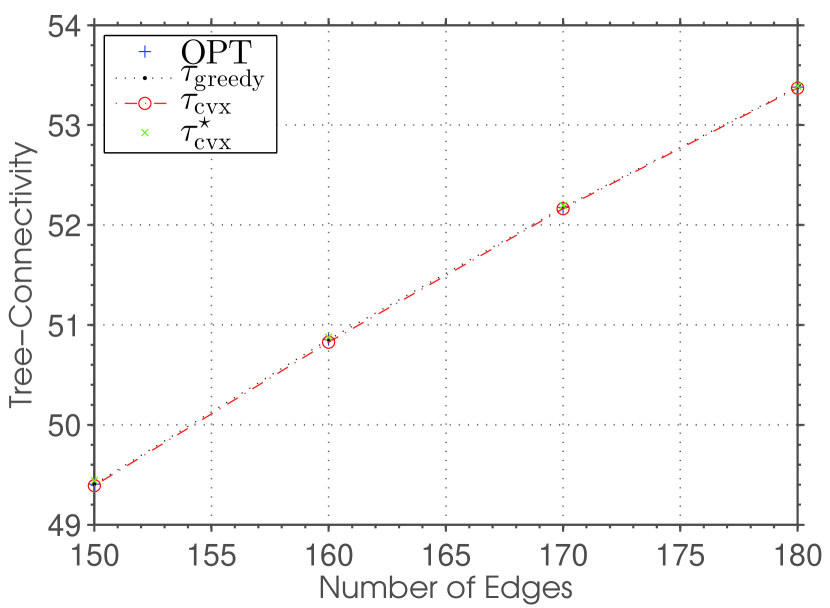
(a) $n=20$, $k=5$

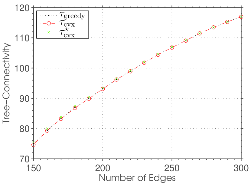
(b) $n=50$, $k=5$

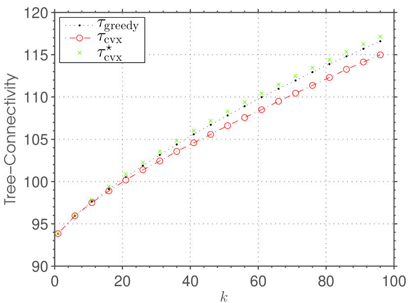
(c) $n=50$, $|{{{\mathcal{E}}}_{\text{init}}}|=200$

Figure 1: $k$-$\mathrm{ESP}^{\texttt{+}}$ on randomly generated graphs with $\mathcal{C}^{\texttt{+}}=\binom{[n]}{2}\setminus{{{\mathcal{E}}}_{\text{init}}}$.

The proposed algorithms were implemented in MATLAB. P₂ is modelled using YALMIP [22] and solved using SDPT$3$ [28].

4.2.1 Random Graphs.

Figure 1 illustrates the performance of our approximate algorithms in randomly generated graphs. The set of candidates in these experiments is $\mathcal{C}^{\texttt{+}}=\binom{[n]}{2}\setminus{{{\mathcal{E}}}_{\text{init}}}$. Figures 1(a) and 1(b) show the resulting tree-connectivity as a function of the number of randomly generated edges for a fixed $k=5$ and, respectively, $n=20$ and $n=50$. Our results indicate that both algorithms exhibit remarkable performances for $k=5$. Note that computing $\mathsf{OPT}$ by exhaustive search is only feasible in small instances such as Figure 1(a). Nevertheless, computing the exact $\mathsf{OPT}$ is not crucial for evaluating our approximate algorithms, as Corollary 3 guarantees that $\tau^{\star}_{\text{greedy}}\leq\mathsf{OPT}\leq{\tau}^{\star}_{\text{cvx}}$; i.e., the space between each black $\mathrm{\cdot}$ and the corresponding green $\times$. Figure 1(c) shows the results obtained for varying $k$. The optimality gap for $\tau_{\text{cvx}}$ gradually grows as the planning horizon $k$ increases. Our greedy algorithm, however, still yields a near-optimal approximation.

4.2.2 Real Pose-Graph Dataset.

We also evaluated the proposed algorithms on the Intel Research Lab dataset as a popular pose-graph SLAM benchmark. In this scenario, ${{{\mathcal{E}}}_{\text{init}}}$ is chosen to be the set of odometry edges, and $\mathcal{C}^{\texttt{+}}$ is the set of loop closures. The parameters in this graph are $n=943$, $|{{{\mathcal{E}}}_{\text{init}}}|=942$ and $|\mathcal{C}^{\texttt{+}}|=895$. Note that computing the true $\mathsf{OPT}$ via exhaustive search is clearly impractical; e.g., for $k=100$, there are more than $10^{134}$ possible graphs. For the edge weights, we are using the original information (precisions) reported in the dataset. Since the translational and rotational measurements have different precisions, two weight functions—$w_{p}$ and $w_{\theta}$—assign weights to each edge of the graph, and the objective is to maximize $2\,\tau_{w_{p}}(\mathcal{G})+\tau_{w_{\theta}}(\mathcal{G})$. Figure 2 shows the resulting objective value for the greedy and convex relaxation approximation algorithms, as well as the upper bounds ($\mathcal{U}$) in Corollary 3. According to Figure 2, both algorithms have successfully found near-$t$-optimal (near-D-optimal) designs. The greedy algorithm has outperformed the convex relaxation with the simple deterministic (sorting) rounding procedure. For small values of $k$, the upper bound $\mathcal{U}$ on $\mathsf{OPT}$ is given by $\mathcal{U}_{\text{greedy}}$ (blue curve). However, for $k\geq 60$, the convex relaxation provides a significantly tighter upper bound on $\mathsf{OPT}$ (green curve). In this dataset, YALMIP+SDPT3 on an Intel Core i5-2400 operating at 3.1 GHz can solve the convex program in about $20$-$50$ seconds, while a naive implementation of the greedy algorithm (without using rank-one updates) can solve the case with $k=400$ in about $25$ seconds.

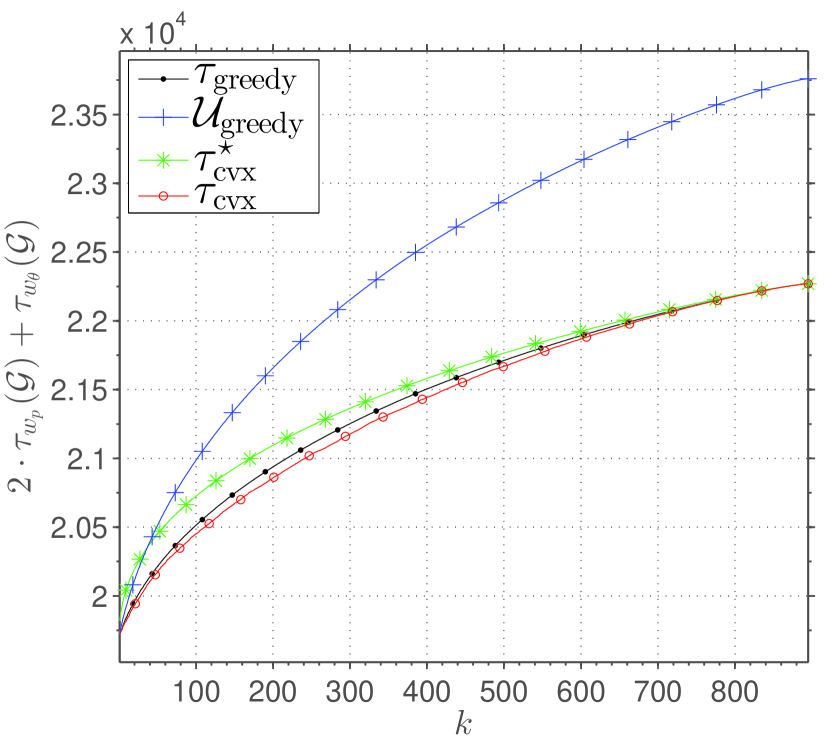
(a) Performance of the proposed approximation algorithms.

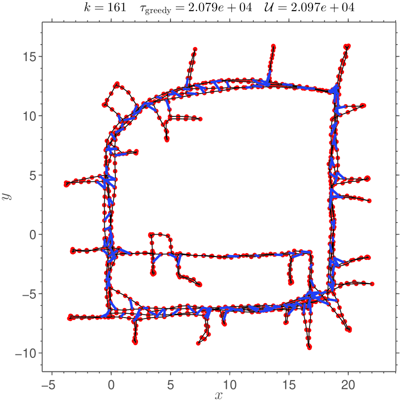
(b) Greedy design for $k=161$ loop closures (out of $895$). Loop-closure edges are shown in blue.

Figure 2: $k$-$\mathrm{ESP}^{\texttt{+}}$ for pose-graph SLAM on the Intel Research Lab dataset.

5 Conclusion

We presented a graph-theoretic approach to the problem of designing sparse reliable (i.e., near-D-optimal) pose-graph SLAM. This paper demonstrated that this problem boils down to a combinatorial optimization problem whose goal is to find a sparse graph with the maximum weighted number of spanning trees. The problem of characterizing $t$-optimal graphs is an open problem with—to the best of our knowledge—no known efficient algorithm. We designed two efficient approximation algorithms with provable guarantees and near-optimality certificates. First and foremost, we introduced a new submodular graph invariant, i.e., weighted tree-connectivity. This was used to guarantee that the greedy algorithm is a constant-factor approximation algorithm for this problem with a factor of $(1-1/e)$ (up to a constant normalizer). In another approach, we formulated the original combinatorial optimization problem as an integer program that admits a natural convex relaxation. We discussed deterministic and randomized rounding schemes. Our analysis sheds light on the connection between the original and the relaxed problems. Finally, we evaluated the performance of the proposed approximation algorithms using random graphs and a real pose-graph SLAM dataset. Although this paper specifically targeted SLAM, we note that the proposed algorithms can be readily used to synthesize near-$t$-optimal graphs in any domain where maximizing tree-connectivity is useful. See, e.g., [10, 20, 3, 19] for applications in Chemistry, RNA modelling, network reliability under random link failure and estimation over sensor networks, respectively.

References

- [1] Bailey, R.A., Cameron, P.J.: Combinatorics of optimal designs. Surveys in Combinatorics 365 (2009) 19–73
- [2] Bauer, D., Boesch, F.T., Suffel, C., Van Slyke, R.: On the validity of a reduction of reliable network design to a graph extremal problem. Circuits and Systems, IEEE Transactions on 34(12) (1987) 1579–1581
- [3] Boesch, F.T., Satyanarayana, A., Suffel, C.L.: A survey of some network reliability analysis and synthesis results. Networks 54(2) (2009) 99–107
- [4] Boyd, S., Vandenberghe, L.: Convex optimization. Cambridge university press (2004)
- [5] Cheng, C.S.: Maximizing the total number of spanning trees in a graph: two related problems in graph theory and optimum design theory. Journal of Combinatorial Theory, Series B 31(2) (1981) 240–248
- [6] Friedman, J., Hastie, T., Tibshirani, R.: Sparse inverse covariance estimation with the graphical lasso. Biostatistics 9(3) (2008) 432–441
- [7] Gaffke, N.: D-optimal block designs with at most six varieties. Journal of Statistical Planning and Inference 6(2) (1982) 183–200
- [8] Ghosh, A., Boyd, S., Saberi, A.: Minimizing effective resistance of a graph. SIAM review 50(1) (2008) 37–66
- [9] Godsil, C., Royle, G.: Algebraic graph theory. Graduate Texts in Mathematics Series. Springer London, Limited (2001)
- [10] Gutman, I., Mallion, R., Essam, J.: Counting the spanning trees of a labelled molecular-graph. Molecular Physics 50(4) (1983) 859–877
- [11] Hochbaum, D.S.: Approximation algorithms for NP-hard problems. PWS Publishing Co. (1996)
- [12] Huang, G., Kaess, M., Leonard, J.J.: Consistent sparsification for graph optimization. In: Mobile Robots (ECMR), 2013 European Conference on, IEEE (2013) 150–157
- [13] Joshi, S., Boyd, S.: Sensor selection via convex optimization. Signal Processing, IEEE Transactions on 57(2) (2009) 451–462
- [14] Kelmans, A.K.: On graphs with the maximum number of spanning trees. Random Structures & Algorithms 9(1-2) (1996) 177–192
- [15] Kelmans, A.K., Kimelfeld, B.: Multiplicative submodularity of a matrix’s principal minor as a function of the set of its rows and some combinatorial applications. Discrete Mathematics 44(1) (1983) 113–116
- [16] Khosoussi, K., Huang, S., Dissanayake, G.: Novel insights into the impact of graph structure on SLAM. In: Proceedings of IEEE/RSJ International Conference on Intelligent Robots and Systems (IROS), 2014. (2014) 2707–2714
- [17] Khosoussi, K., Huang, S., Dissanayake, G.: Good, bad and ugly graphs for SLAM. RSS Workshop on the problem of mobile sensors (2015)
- [18] Khosoussi, K., Huang, S., Dissanayake, G.: Tree-connectivity: A metric to evaluate the graphical structure of SLAM problems. Proceedings of the IEEE International Conference on Robotics and Automation (ICRA) (2016)
- [19] Khosoussi, K., Sukhatme, G.S., Huang, S., Dissanayake, G.: Maximizing the weighted number of spanning trees: Near--optimal graphs. arXiv:1604.01116 (2016)
- [20] Kim, N., Petingi, L., Schlick, T.: Network theory tools for RNA modeling. WSEAS transactions on mathematics 9(12) (2013) 941
- [21] Kretzschmar, H., Stachniss, C., Grisetti, G.: Efficient information-theoretic graph pruning for graph-based slam with laser range finders. In: Intelligent Robots and Systems (IROS), 2011 IEEE/RSJ International Conference on. (2011) 865 –871
- [22] Löfberg, J.: Yalmip : A toolbox for modeling and optimization in MATLAB. In: Proceedings of the CACSD Conference, Taipei, Taiwan (2004)
- [23] Myrvold, W.: Reliable network synthesis: Some recent developments. In: Proceedings of International Conference on Graph Theory, Combinatorics, Algorithms, and Applications. (1996)
- [24] Nemhauser, G.L., Wolsey, L.A., Fisher, M.L.: An analysis of approximations for maximizing submodular set functions - I. Mathematical Programming 14(1) (1978) 265–294
- [25] Petingi, L., Rodriguez, J.: A new technique for the characterization of graphs with a maximum number of spanning trees. Discrete mathematics 244(1) (2002) 351–373
- [26] Shamaiah, M., Banerjee, S., Vikalo, H.: Greedy sensor selection: Leveraging submodularity. In: 49th IEEE conference on decision and control (CDC), IEEE (2010) 2572–2577
- [27] Shier, D.: Maximizing the number of spanning trees in a graph with n nodes and m edges. Journal Research National Bureau of Standards, Section B 78 (1974) 193–196
- [28] Tütüncü, R.H., Toh, K.C., Todd, M.J.: Solving semidefinite-quadratic-linear programs using sdpt3. Mathematical programming 95(2) (2003) 189–217
- [29] Vandenberghe, L., Boyd, S., Wu, S.P.: Determinant maximization with linear matrix inequality constraints. SIAM journal on matrix analysis and applications 19(2) (1998) 499–533
- [30] Weichenberg, G., Chan, V.W., Médard, M.: High-reliability topological architectures for networks under stress. Selected Areas in Communications, IEEE Journal on 22(9) (2004) 1830–1845