The Gaia-ESO Survey: the inner disk, intermediate-age open cluster Trumpler 23

Abstract

Context. Trumpler 23 is a moderately populated, intermediate-age open cluster within the solar circle at a R${}_{\mathrm{GC}}\sim$ 6 kpc. It is in a crowded field very close to the Galactic plane and the color-magnitude diagram shows significant field contamination and possible differential reddening; it is a relatively understudied cluster for these reasons, but its location makes it a key object for determining Galactic abundance distributions.

Aims. New data from the Gaia-ESO Survey enable the first ever radial velocity and spectroscopic metallicity measurements for this cluster. We aim to use velocities to isolate cluster members, providing more leverage for determining cluster parameters.

Methods. Gaia-ESO Survey data for 167 potential members have yielded radial velocity measurements, which were used to determine the systemic velocity of the cluster and membership of individual stars. Atmospheric parameters were also used as a check on membership when available. Literature photometry was used to re-determine cluster parameters based on radial velocity member stars only; theoretical isochrones are fit in the $V$, $V-I$ diagram. Cluster abundance measurements of ten radial-velocity member stars with high-resolution spectroscopy are presented for 24 elements. These abundances have been compared to local disk stars, and where possible placed within the context of literature gradient studies.

Results. We find Trumpler 23 to have an age of 0.80 $\pm$ 0.10 Gyr, significant differential reddening with an estimated mean cluster E($V-I$) of 1.02${}^{+0.14}_{-0.09}$, and an apparent distance modulus of 14.15 $\pm$ 0.20. We find an average cluster metallicity of [Fe/H] = 0.14 $\pm$ 0.03 dex, a solar [$\alpha$/Fe] abundance, and notably subsolar [s-process/Fe] abundances.

1 Introduction

Open clusters (OCs) are very useful tools for the study of physics on stellar and Galactic scales. The astrophysical properties of stars can be isolated by studying a single-age population of stars in multiple evolutionary states; nucleosynthesis can also be probed with precise measurements of abundances of clusters in different age ranges. Because the dispersion in abundances between unevolved stars in a single cluster is typically small or nonexistent (see, e.g., Randich et al. 2006; De Silva et al. 2006; Liu et al. 2016), many cluster stars can be used to gain a more accurate measurement of the primordial cluster abundance. Since a cluster is composed of a single age population, the evolutionary states of stars can be relatively easily determined with a color-magnitude diagram. Cluster parameters (age, distance, reddening, metallicity) can also be determined in this way, allowing clusters to be placed within the larger context of the evolution of the Galaxy.
A current topic of active research is the determination of radial abundance gradients for various groups of chemical elements across different regions of the Galactic disk. Open clusters and field stars can both be used as tracers of the chemical history of the disk, but clusters have more easily determined ages and distances, putting constraints on different epochs of Galaxy formation. They are also found at a large range of Galactocentric radii and ages, ranging from millions of years old to approximately 10 Gyr old (Salaris et al. 2004) and $\sim$5 to 24 kpc from the center of the Galaxy (Magrini et al. 2010; Carraro & Costa 2007). Recent efforts have been made to provide a uniform age scale for OCs (Salaris et al. 2004; Bragaglia & Tosi 2006), and to probe the outer regions of the disk (e.g., Carraro et al. 2004; Bragaglia et al. 2008; Sestito et al. 2008; Yong et al. 2012; Cantat-Gaudin et al. 2016), the solar neighborhood (e.g., Frinchaboy et al. 2013), and the inner disk (Magrini et al. 2010; Jacobson et al. 2016). However, relatively few OCs well inside the solar circle (R_GC $<$ 7 kpc) have parameter determinations due to observational challenges, and the measurements that do exist can be difficult to compare from study to study.
Several large studies address the need for observational data of many clusters exploring the Galactic parameter space on a common analysis and abundance scale, such as RAVE (Conrad et al. 2014), LAMOST (Deng et al. 2012), OCCASO (Casamiquela et al. 2016), and OCCAM as part of APOGEE (Frinchaboy et al. 2013; Cunha et al. 2016). The Gaia-ESO Survey (GES) is a public spectroscopic survey of stars in all components of the Milky Way using VLT FLAMES planned as a complement to the Gaia mission (Gilmore et al. 2012; Randich et al. 2013). Observations and data analysis are currently underway, and the completed survey will cover some 100,000 stars in the Galaxy and $\sim$70 OCs. The GES will measure at least 12 elements (Na, Mg, Si, Ca, Ti, V, Cr, Mn, Fe, Co, Sr, Zr, and Ba) for a few thousand field stars and the full sample of OCs with high-resolution spectroscopy. This is one of a series of papers on OC data obtained and analyzed by GES focusing on the intermediate-age inner disk cluster Trumpler 23.
Trumpler 23 is a moderately well-populated OC located in the 4th quadrant of the Galaxy at $l$ = 328.86^∘, $b$ = -0.47^∘, close to the plane of the Galaxy toward the Galactic center. It is approximately 0.6 Gyr old and 2 kpc from the Sun (Carraro et al. 2006), well inside the solar circle at an R_GC $\sim$ 6 kpc. Due to previously noted complications with crowding, differential reddening (DR) and possible tidal effects (Bonatto & Bica 2007) membership determination via photometry is difficult and no previous spectroscopic studies exist. However, its location and characteristics make it an interesting candidate for further study. The GES is well positioned to take full advantage of Tr 23 observations because of its uniform data analysis pipelines and large potential number of comparison clusters at various Galactocentric radii (Magrini et al. 2014, Jacobson et al. 2016).
The paper is structured as follows: in Section 2 we review previous literature studies of Trumpler 23; in Section 3 we describe the structure of the Gaia-ESO Survey and observations; in Section 4 we perform radial velocity membership selection; in Section 5 we detail atmospheric parameter determinations of target stars; in Section 6 we determine our own set of cluster parameters using literature photometry; in Section 7 we discuss abundance measurements; and in Section 8 we summarize our points and conclude.

2 Cluster parameters from the literature

Trumpler (1930) first described Tr 23 as a sparse cluster of relatively faint stars not easily distinguished from its surroundings. The first data on Tr 23 were provided by van den Bergh & Hagen (1975) as part of a two-color survey of southern OCs; they classified it as a moderately well-populated cluster with a diameter of 6$\arcmin$.
There are two existing photometric studies of Trumpler 23 by Carraro et al. (2006) and Bonatto & Bica (2007). Carraro et al. obtained Johnson-Cousins $V,I_{c}$ photometry for $\sim$11000 stars in the field of Tr 23. They noted that the main sequence is unusually broad, which they attributed to DR or perhaps a high cluster binary fraction. They also pointed out that Tr 23 may be undergoing strong tidal interactions with the Galaxy because of its apparent elongated shape on the sky. They used Padova isochrones (Girardi et al. 2000a) to estimate a cluster age of 0.6 $\pm$ 0.1 Gyr assuming solar metallicity, although they noted that the age could vary from 0.5 to 1.5 Gyr depending on the true cluster metallicity. They also found a high reddening E($V-I$) = 1.05 $\pm$ 0.05 (converted to an E($B-V$) = 0.84), and derived cluster parameters of (m $-$ M)_V = 14.35 $\pm$ 0.20, and d_⊙ = 2.2 kpc (corresponding to a Galactocentric radius of 6.2 kpc if R_⊙ = 8.0 kpc).
Bonatto & Bica (2007) examined six clusters inside the solar circle that are located in crowded fields, including Tr 23. They used 2MASS $J$, $H$, and $K_{s}$ photometry to correct for field contamination and derive cluster parameters for Tr 23. In the cleaned CMD, the Tr 23 main sequence in $J$, $J-H$ is still unusually broad. The authors found evidence of DR in an 80$\arcmin$ $\times$ 80$\arcmin$ field around Tr 23. The profile of the cluster after color-magnitude filtering is irregular across declination, and field star counts drop significantly toward higher declinations. The radial distribution of assumed photometric members in the Tr 23 field is not well-fit by a two-parameter King model, and does not appear to be a smooth distribution, which they also attribute to significant DR. The authors also noted that the inner disk clusters studied have unusually high mass densities and small limiting radii compared to solar neighborhood OCs, which would suggest strong Galactic tidal effects on Tr 23. Using Padova isochrones of solar metallicity as in Carraro et al. (2006), they found a significantly lower reddening of E($B-V$) = 0.58 $\pm$ 0.03, an age of 0.9 $\pm$ 0.1 Gyr, and a distance d_⊙ = 1.9 $\pm$ 0.1 kpc.

3 Observations

3.1 Gaia-ESO survey methods

Data for GES are taken with FLAMES (Fiber Large Array Multi-Element Spectrograph) on the VLT at the European Southern Observatory. FLAMES has two instruments, the medium-resolution multi-object spectrograph GIRAFFE and the high-resolution UVES (Ultraviolet and Visual Echelle Spectrograph) (Pasquini et al. 2002). The target selection, observation, data reduction, atmospheric parameter determination, and abundance measurements are handled by specific working groups (WGs) within the collaboration. Parameter and abundance determinations for each target are typically done by multiple subgroups within WGs called abundance analysis nodes, and the results of individual nodes are combined within each WG; the WG values are then homogenized to yield final recommended parameters. This structure produces homogenous parameter determinations while allowing WGs to specialize in different types of stars. The data described here come from the fourth internal data release (GESviDR4Final) which comprises a (re-)analysis of all available spectra taken before July 2014 using an updated linelist (Heiter et al. 2015) and analysis techniques. For more details about the data reduction, which will not be discussed here, see Sacco et al. (2014) and Lewis et al. (in prep).
Analysis of the GIRAFFE FGK star atmospheric parameters and abundances (using solar abundances by Grevesse et al. 2007) is handled by WG 10 (Recio-Blanco et al., in prep), UVES FGK star parameters and abundances by WG 11 (Smiljanic et al. 2014), and the homogenization of results from different subgroups by WG 15 (Hourihane et al., in prep). Smiljanic et al. (2014) describes in detail the methods used by individual nodes and the process of obtaining stellar parameters and abundances for FGK stars using UVES data. Multiple WG11 nodes measure abundances and atmospheric parameters using the same atomic data, solar abundances, and model atmospheres, but different methods. Some nodes determine atmospheric parameters using equivalent widths and minimizing abundance trends with excitation potential, line strength, etc., and some nodes compare observed spectra to spectral libraries. For abundance determinations, some nodes use automated or semi-automated equivalent width determinations and some use spectral synthesis software. The abundance homogenization process of GES makes use of a number of calibrating objects (clusters with many stars) to assess the precision of each abundance analysis technique, and Gaia benchmark stars (individually well-studied stars with independently determined atmospheric parameters) to test the accuracy of abundance measurements and atmospheric parameters (Pancino et al., in prep.). Node measurements of benchmark and calibration stars are used to evaluate the performance of each node in different parameter spaces; a final WG value for each star is determined by weighting each node’s value by its accuracy in determining benchmark parameters. These weights are also used in determining final abundances. The evaluation of calibration and benchmark star abundances determined by individual nodes also ensure that uncertainties given for stellar abundances reflect the inherent uncertainties in the various measurement techniques.

3.2 Target selection for GES

For intermediate-age OCs with prominent red clumps, GES targets are selected as follows: likely clump stars are observed with UVES, so that the most time-intensive targets are most likely to be members, followed by probable red giants if the clump is sparse. Main sequence stars down to $V$ = 19 are observed with GIRAFFE, using the HR9B setup primarily for stars of spectral type A to F and the HR15N setup for cooler stars. General GES target selection methods are outlined in Bragaglia et al. (in prep.).
The field of Tr 23 is crowded, reaching 50% field star contamination at 5$\arcmin$ (Carraro et al. 2006); careful target selection is required. Targets were chosen based on both the Carraro et al. (2006) $VI$ photometry and 2MASS $J$, $H$, and $K$. 151 apparent main-sequence and giant stars were selected as GIRAFFE targets with 13.5 $<$ $V$ $<$ 18 within 6$\arcmin$ of the cluster center in order to limit field contamination, which increases with both distance from the cluster center and $V$ magnitude. Tr 23 has a distinct red clump with relatively high membership probabilities, so 16 stars out of 21 in or near the clump and within 6$\arcmin$ of the cluster center were selected as UVES targets.
Data were taken on the nights of 28 and 29 July and 13 and 14 September 2013. 54 GIRAFFE targets were observed with the HR15N setup only (6470-6790$\rm\AA$ and R = 17,000), 81 stars were observed with the HR9B setup only (5143-5356$\rm\AA$ and R = 25,900), and 16 targets were observed with both. UVES targets were observed with the U580 setup (4800-5800$\rm\AA$ and R = 47,000). The typical signal-to-noise ratios achieved for the HR15N, HR9B, and U580 setups are $\sim$160, 60, and 90, respectively. The CMD and coordinates of target stars are shown in Figure 1.

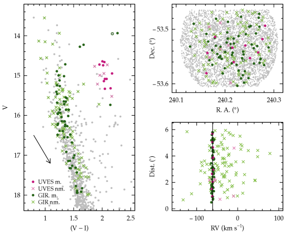
Figure 1: Left: CMD of Trumpler 23 of photometry from Carraro et al. (2006) with all stars within 6$\arcmin$ marked as small grey dots, UVES cluster members as purple circles, UVES non-members as light purple crosses, GIRAFFE cluster members as dark green circles, and GIRAFFE non-members as light green crosses. Star 18, targeted by GIRAFFE, is a cluster member by radial velocity but has inconsistent atmospheric parameters (see Section 6) so it is marked with an open green circle. A reddening vector is also marked in the lower left. Top right: the same symbols showing the coordinates of all stars observed in the Gaia-ESO survey and Carraro et al. (2006) stars within 6$\arcmin$. Lower right: the same symbols showing distance from the cluster center vs. radial velocity of all observed stars except for one GIRAFFE non-member at +459 km s^-1. The cluster systemic velocity is marked as a solid line.

4 Membership determination

Because Tr 23 has heavy field star contamination, radial velocities are very important in determining membership. GIRAFFE radial velocities have a typical error of $\sim$0.4 km s^-1, although stars with the highest rotational velocities or lowest SNR have errors up to several km s^-1 (Jackson et al. 2015); UVES radial velocity errors are around 0.6 km s^-1  (Sacco et al. 2014). Figure 2 shows a histogram of UVES and GIRAFFE target velocities from $-140$ to 80 km s^-1 (excluding the most discrepant GIRAFFE star). There is a clear peak in the velocity distribution around $-60$ km s^-1, but a wide range of field star velocities. Using an iterative 2$\sigma$ clipping technique on the mean until $<5\%$ of stars were eliminated as outliers (13 iterations), we have determined a cluster velocity of $-61.3\pm 1.9$ km s^-1 (s.d.) from 70 member stars within 2$\sigma$ of the mean. Thus, ten out of the total of 16 UVES target stars have radial velocities consistent with the cluster compared to 60 out of 151 GIRAFFE targets (20 observed with HR15N setup only, 21 observed with HR9B setup only, and nine observed with both). The cluster radial velocity dispersion of 1.9 km s^-1  is slightly higher than typical for OCs; Mermilliod et al. (2009) find a typical dispersion on cluster radial velocities of $\sim$1 km s^-1. However, considering the errors on the velocities and possible contamination by field stars and unresolved binaries, this is a reasonable dispersion.
As is clear from Fig. 2, the field of Tr 23 has a significant number of field stars at a range of radial velocities, some of which will fall within the cluster radial velocity range (the minimum radial velocity of member stars selected by sigma clipping is $-64.9$ km s^-1 and the maximum is $-57.3$ km s^-1). We have used a Besançon star count model (http://model.obs-besancon.fr/) to estimate the number of field stars falling within the cluster radial velocity limits (Robin et al. 2003). Figure 2 shows the observed radial velocity distribution overlaid with the field radial velocity distribution predicted by the model. The predicted distribution is scaled to the total number of stars observed divided by the number of stars in the Carraro et al. (2006) photometry in the same $V$ mag range. The scaled model predicts that $\sim$15 field stars fall within the selected bounds of the cluster radial velocity distribution. This is a rough scaling, but it reproduces reasonably well the field star velocity distribution, including the long tail of the observed field star distribution toward higher radial velocities typically observed in the disk. The reverse scenario, where member stars which are spectroscopic binaries happen to fall outside of the cluster radial velocity distribution, is also possible; however, this possibility will not affect conclusions drawn in this work.

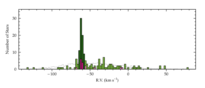
Figure 2: Stellar radial velocity distribution of GIRAFFE and UVES target objects using the same color scheme as in Figure 1. The dotted line represents a Besançon star count model for the same field as the Carraro et al. (2006) photometry, scaled as the number of field stars observed in GES divided by the total number of field stars in the same color and magnitude range.

5 Atmospheric parameters

Effective temperatures were determined for 31 of the 60 GIRAFFE radial velocity members; atmospheric parameters (when available) are listed along with metallicities, coordinates, photometry, and velocities in Table 1 (here and in other tables and figures we use $\xi$ to represent microturbulent velocity). Due to methods of pipeline analysis and limitations of the data, some GIRAFFE stars do not have atmospheric parameter determinations, or only partial parameter sets. 46 out of 91 GIRAFFE radial velocity non-members also have at least partial parameter determinations; these are given in Table 2.
Figure 3 shows UVES [Fe/H] plotted against radial velocities for 14 UVES targets with fully determined parameters; two UVES targets with highly discrepant radial velocities are not shown. Radial velocity (RV) members are marked as filled circles, potential binary members as open circles, and non-members as crosses. Dashed lines indicate the UVES member mean values and dotted lines mark 2$\sigma$ from the mean.
Star 74 has a radial velocity 3$\sigma$ from the determined cluster velocity, and star 86 is 2.5$\sigma$ from the cluster radial velocity. Stars 74 and 86 may be binary members, but we will consider them non-members for the purpose of evaluating cluster parameters. Stars 56, 89, 131, and 147 are more than 4$\sigma$ from the mean cluster radial velocity, so we consider them non-members. Table 3 gives UVES target photometry, coordinates, radial velocities, atmospheric parameters, and membership status.
The weighted mean [Fe/H] of the ten UVES radial velocity cluster members is 0.14 $\pm$ 0.03 (s.d.), with a typical stellar [Fe/H] error of 0.10 dex. The weighted mean of the 20 GIRAFFE radial velocity cluster members with abundance determinations is 0.15 $\pm$ 0.17 (s.d.) with a typical stellar [Fe/H] error of 0.28 dex. The two determinations show excellent agreement, suggesting that the sometimes systematic differences in UVES and GIRAFFE abundances seen in earlier releases have been eliminated. The weighted average of both the UVES and GIRAFFE radial velocity member [Fe/H] is 0.14, with an error on the mean of 0.03 dex; we have adopted this as the cluster [Fe/H].
With a Galactocentric distance of only 6 kpc, Tr 23 is one of the few intermediate-age clusters we can use to probe the inner Galactic disk. Its clear super-solar metallicity makes it especially interesting in the context of the behavior of the abundance gradient inside the solar circle. Magrini et al. (2010), from a new sample of three inner disk open clusters, along with a selection of clusters from the literature, found evidence that the gradient increased strongly toward the Galactic center, but their sample included only one cluster inside 6.5 kpc, and only three inside 7 kpc. The GES survey now provides abundances on a uniform metallicity scale for nine clusters inside this limit, with Tr 23 being among the three closest to the Galactic center. As shown in Jacobson et al. (2016), this GES cluster sample can be described by a linear relationship of increasing metallicity with decreasing Galactocentric distance with a slope of -0.10 $\pm$0.02 dex kpc^-1. The abundance of Tr 23 falls neatly on this relationship, substantiating the gradual rather than a steepening increase in metallicity in these innermost regions.

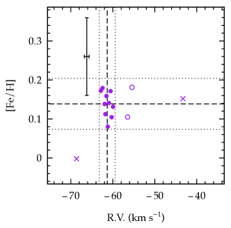
Figure 3: UVES target [Fe/H] against radial velocity. Ten RV members are marked as filled circles, two possible binary members as open circles, and two non-members as crosses (two additional non-members lie outside the bounds of this plot). Dashed and dotted lines indicate the mean and 2$\sigma$ boundaries respectively.

6 Re-determined cluster parameters

With radial velocity membership and [Fe/H] determinations as a guide, we have determined a refined set of cluster parameters from the member CMD. Member selection narrows the main sequence (MS) somewhat (see Fig. 1), although the width still allows for some degeneracy in CMD fitting. Carraro et al. (2006) suggest that stars in the field of Tr 23 past the main-sequence turn-off (TO) might be blue stragglers, but all of the objects observed by GES in this region are radial velocity non-members, so these may in fact be mostly field stars. None of the seven potential blue stragglers observed have determined metallicities; only one has a RV within 4$\sigma$ of the cluster average, and the others are more than 10$\sigma$ from the cluster RV. There are also four GIRAFFE radial velocity members that appear to be evolved stars based on their photometry. Two of these stars have determined atmospheric parameters: one appears to be on the subgiant branch and has parameters that are consistent with its location on the CMD. The other, star 18, which is marked as an open circle in Figure 1, appears to be on either the giant branch or AGB but has parameters that would indicate it is actually a dwarf; it is likely an interloper hidden in the radial velocity distribution of the cluster. We did not include this star in the isochrone fitting. The two apparent giants without atmospheric parameter determinations were treated as members.
The red clump is pronounced and well-populated, but also appears unusually extended, covering $\sim$0.7 magnitudes in $V$ and 0.3 in $V-I$. As mentioned above, the width of the MS ($\sim$0.2 in $V-I$) is much larger than the photometric errors for $V$ $<$ 18, and may be attributable to DR or a high cluster binary fraction. We discuss the binary possibility at the end of the section. If the cause of the width of the MS is DR, one might expect stars on the redder side of the MS to appear in different locations on the sky than stars on the apparent blue side of the MS. Figure 4 shows main sequence members with 16 $<$ $V$ $<$ 18 divided into two groups, a blue edge and red edge of the MS, and the location of stars in these two groups on the sky. The two color groups appear to separate into four stripes on the sky, with the DR mainly occurring along the declination axis as found by Bonatto & Bica (2007), although the size of the cluster (and the plot in Figure 4) is significantly smaller than the $80\arcmin\times 80\arcmin$ area on the sky they use to examine the DR. The Galactic plane is at an angle of $\sim$ -27^o from the axis of right ascension in this figure, so the direction of the DR corresponds to Galactic latitude, with stars on the red edge of the MS appearing in two groups at higher average latitudes than stars on the blue edge of the MS. At a distance of 2.2 kpc the angular extent of radial velocity members corresponds to 6 parsecs. Tr 23 is only 50 pc above the plane, so it is likely that reddening would vary with shallow angles out of the plane; DR of this magnitude (A${}_{V}\sim 0.5$) in the direction of the bulge has been reported across small fields on the order of parsecs (Ortolani et al. 1990; Gonzalez et al. 2012). The spread in $V$ and $V-I$ of the clump also roughly correspond with the dimensions of the reddening vector shown in Figure 1 (left panel).

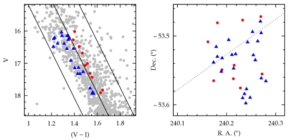
Figure 4: Left: a zoomed-in version of the CMD in Figure 1, with possible blue and red main sequences marked as triangles and circles. Right: plot of the right ascension and declination of these stars using the same symbols for each group, with a dotted line marking constant Galactic latitude b = -0.47.

We have attempted to correct for DR in the field of Tr 23. For a complete discussion of the methods used, we refer the reader to Donati et al. (2014); briefly, we selected an area of the MS below the TO but above areas of highest field contamination and set a fiducial line along the MS, then iteratively calculated the median DR for each MS star and a group of its nearest neighbors, and binned the results on the sky to get the final corrections. However, our corrections for the DR effects did not yield a marked improvement in the definition of the MS when considering all stars in the field or the member stars only (which go out to 6$\arcmin$ from the cluster center; see Fig. 1). Therefore, we fitted isochrones and derived cluster parameters based on the uncorrected photometry, fitting the blue edge of the MS which seems reasonably well defined. We do not have membership determinations for enough clump stars to look at the possibility of DR as a cause of its extended $V$ mag range, but seven of the ten apparent clump stars fall in a fairly narrow range in $V-I$ of 2.00 to 2.08. We can thus use the red clump for a reasonable assessment of the general reddening across Tr 23, though we estimate the error in the reddening conservatively. The algorithm we use for the DR correction does consistently estimate a reddening variability of $\pm$0.1 in $V-I$, which matches well the width of the clump in $V-I$ and our estimated uncertainty on our E($V-I$) discussed below.
We have used PARSEC (Bressan et al. 2012), BaSTI (Pietrinferni et al. 2004), and Dartmouth (Dotter et al. 2008) isochrones to determine the age, reddening, and distance of Tr 23 based on the selected member stars and cluster metallicity. Metallicity values were set relative to a solar Z = 0.0152 where possible; an input of Z = 0.021 was used for the PARSEC and Dartmouth models, and the closest option of Z = 0.0198 was selected for the BaSTI models. The isochrones were also selected to have a solar [$\alpha$/Fe] ratio (see Section 7.2). Figure 5 shows the cluster CMD with Carraro et al. (2006) photometry for stars within 6$\arcmin$ of the cluster center in gray, cluster members as black circles, non-members as orange dots, and selected isochrones for each model set in blue, with intervals corresponding to $\pm$0.1 Gyr in red and green. Table 4 gives the best fit parameters for each isochrone, and values found in the literature.

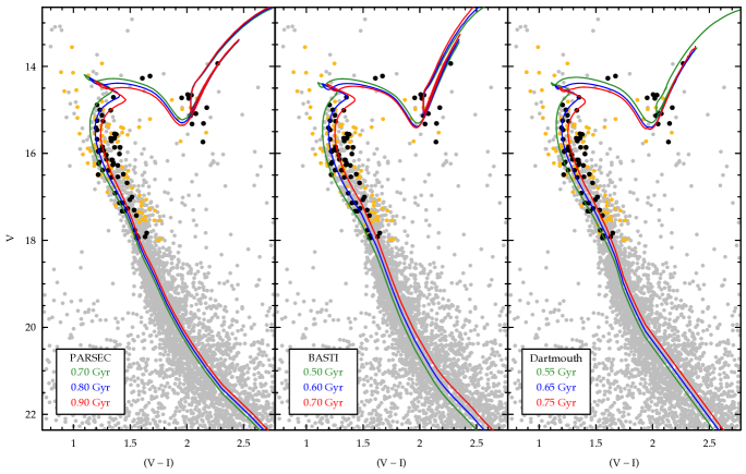
Figure 5: Tr 23 CMD with Carraro et al. (2006) photometry in grey, cluster members in black circles, non-members in orange dots, and isochrones. Left panel is PARSEC isochrones of 0.7, 0.8, and 0.9 Gyr; middle panel is BASTI isochrones of 0.5, 0.6, and 0.7 Gyr; right panel is Dartmouth isochrones of 0.55, 0.65, and 0.75 Gyr in green, blue, and red, respectively. Adopted reddening and distance moduli are given in Table 4.

The PARSEC 0.8 Gyr isochrone provides a good fit to the TO and a reasonable fit to the blue edge of the lower MS. The reddening can be adjusted to provide a good fit to the center of the red clump, as well as the star that appears to be on the red giant branch. The E($V-I$) for this fit is 1.02${}^{+0.14}_{-0.09}$, where errors are based on fitting either edge of the clump as defined by the ten UVES radial velocity members; two of these that are separated from the group in ($V-I$) cannot be well fit by any of the isochrones while also fitting the main clump. This is likely due to DR, so the errors on our reddening estimates encompass the DR effects on the field. We have used the extinction coefficients of Dean et al. (1978) to derive an E($B-V$) of 0.82${}^{+0.11}_{-0.08}$. The apparent distance modulus for this fit is (m-M)_V = 14.15, with a corresponding solar distance of 2.1 kpc.
The BaSTI 0.6 Gyr isochrone provides a good fit to the lower main sequence and TO region, but the giant and subgiant branches are not as well fit. Here, we use the BaSTI models with convective overshooting in order to obtain a good fit to the lower main sequence. The E($V-I$) required to match this isochrone to the red clump is 1.09${}^{+0.14}_{-0.09}$ with a corresponding E($B-V$) of 0.87${}^{+0.11}_{-0.08}$. The best fit distance modulus is 14.50 (d_⊙ = 2.3 kpc).
The Dartmouth 0.65 Gyr isochrone fits the turnoff region well, but the blue side of the lower main sequence is not well reproduced, and the red clump and AGB do not fit some stars. The 0.65 Gyr isochrone results in a E($V-I$) of 1.10${}^{+0.14}_{-0.09}$ and an E($B-V$) of 0.88${}^{+0.11}_{-0.08}$. The best fit distance modulus is (m-M)_V = 14.45 (d_⊙ = 2.2 kpc). The distance moduli and solar distances we have derived from each of the three models are thus also in agreement.
We can check the ages we have determined with each set of isochrones by plotting HR diagrams. Figure 6 shows the same models as in Figure 5 in log(g) vs. T_eff space, with GIRAFFE and UVES stars with atmospheric parameter determinations overplotted. The errors on many of the points are large enough that these diagrams are not extremely useful in determining the age, but all stars are consistent with these sets of parameters within their error bars and the uncertainties on the isochrone age. The PARSEC isochrones fit the clump star gravities better than the BaSTI and Dartmouth models, which appear to slightly underestimate clump gravities by $\sim$0.1 dex. We can also check our reddening determination with UVES effective temperatures; using the color-temperature relations of Alonso et al. (1999), we find $V-I$ colors for UVES member stars and use these to find a simple reddening estimate. In this way we find a typical E($V-I$) of 1.09 $\pm$ 0.07 (s.d.). This is consistent with the reddening derived by isochrone fitting for all three sets of isochrones, with a range in calculated E$(V-I)$ of 0.19. Errors in effective temperature of $\sim$100 K could also change the calculated E($V-I$) by 0.04 mag.

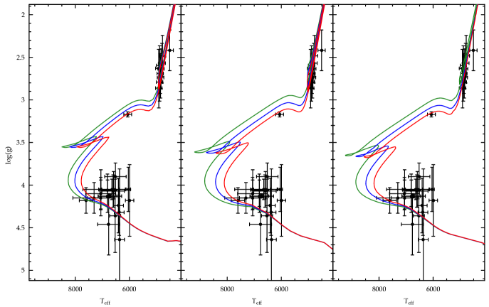
Figure 6: Tr 23 gravities vs. effective temperatures of cluster members in black with isochrones. Panels and lines the are same as in Figure 5.

It is notable that, although the UVES member stars occupy a small range in temperature ($\sim$150K excluding a single outlier in Fig. 3), there is a spread in log(g) of about 0.4 dex. The typical errors on stellar gravities for the UVES stars are $\sim$0.2 dex, so this is not a highly significant spread, but it is also worth considering the evolutionary effects that might cause a real spread in red clump gravities. Girardi et al. (2000b) examine the $V$ magnitude spread in clump stars in OCs NGC 752 and NGC 7789, and postulate that although OCs show no evidence of different age stellar populations that would lead to a stellar mass difference large enough to cause a separation in the clump, mass loss on the RGB is not well understood and it may be possible that some stars in an intermediate age OC would lose enough mass to undergo a helium flash while other cluster stars with slightly more mass would not. Stars that do experience a helium flash would of course be significantly more luminous than those that do not, and this effect would cause a difference in the $V$ magnitude of the lower mass stars as well. The limit for core helium flash to occur is $\sim$2.0 M_⊙, and our model isochrones predict a clump star mass for Tr 23 of 2.3 to 2.5M_⊙ without significant mass loss. This effect of a secondary red clump has only been observed in clusters older than 1 Gyr, most recently in NGC 419 ($\sim$1.4 Gyr; see Girardi et al. 2009), so this is a less likely explanation for the $V$ mag dispersion of the clump than DR or binary stars. There are several evolutionary effects that would cause mass loss prior to the red clump stage (see Donati et al. 2014), but these scenarios still would not involve mass loss of the degree necessary for an OC $<$ 1 Gyr old.
For all three models we estimate an error on the ages of 0.1 Gyr, as that is the smallest difference that visibly affects the quality of the fit given the width of the main sequence. The ages we have derived using the three different sets of isochrones are consistent with each other, as are the reddenings. The error on the distance modulus is difficult to determine given the width of the MS and $V$ mag range of the clump, but we have chosen 0.2 mag because that is the amount required to shift the isochrone vertically by the margin seen in the example fits to the MS in Fig. 5. This results in an error on the solar distance of 0.2 kpc, and an error on the Galactocentric distance of 0.15 kpc. None of the three models fit the member photometry perfectly, but the PARSEC models provide the best overall fit, so we adopt a cluster age of 0.8 $\pm$ 0.1 Gyr, an apparent distance modulus of 14.15 $\pm$ 0.20, and a solar distance of 2.10 $\pm$ 0.20 kpc.
These cluster parameters are consistent with those in the literature except for the reddening; the PARSEC E($B-V$) of 0.82${}^{+0.11}_{-0.08}$ is consistent with the Carraro et al. (2006) value but not the Bonatto & Bica (2007) E($B-V$) of 0.58. As the cluster appears to have variable reddening, it is perhaps not surprising that the calculated reddening would vary depending on the fitting method. Even with member selection, the MS is still broad in ($J-H$) and the clump spreads across $\sim$0.7 mag in $J$. Fitting isochrones to $J$, $J-H$ and $J$, $J-K$ space gives little additional leverage on cluster parameters, partly because of the lack of narrowing in the clump and MS and partly because models predict less change in these colors with cluster age, so we do not utilize this parameter space. It is useful to note that since none of the studies of Tr 23 use $B$ photometry, these E($B-V$) values are subject to differences in color conversions. When fitting isochrones to the 2MASS photometry of members we observe an E($J-H$) of 0.21 for Tr 23 while Bonatto & Bica (2007) find an E($J-H$) of 0.18; this is within the errors we would expect due to the size of the clump in ($J-H$) of $\sim$0.1 mag.
It would seem that the field of Tr 23 either has strong DR or the width of the MS is caused by effects unrelated to extinction. The width of the lower member MS in both ($V-I$) and ($J-H$) might be explained by binaries, as a variation in $V$ of 0.75 mag caused by pairs of equal-mass stars would encompass most member stars with $V$ below 16. However, there is a clump of stars with 15.5 $<$ $V$ $<$ 16 that are too far from the MS to be fully explained by binary stars. If we assume that the separation between the two apparent main sequences shown in Fig. 4 is entirely due to binaries, the binary fraction of the cluster would be at least 30%. This would appear to require the maximum separation of 0.7 mag (i.e., equal mass stars) for most of the ten stars we have marked as the reddened MS, so the actual binary fraction of the cluster might be significantly higher. Observational estimates of the fraction of short-period ($<$ 10⁴ days) binaries in OCs typically fall at $\sim$20% (Duchêne et al. 1999; Mermilliod et al. 2008; Milliman et al. 2014); total binary fractions may be substantially higher. A mixture of DR and binary widening of the MS is perhaps the most likely scenario, and could explain well the full extent of the MS; however, the two effects are difficult to disentangle without more extensive cluster membership data.

7 Abundance analysis

Tables 5, 6, and 7 give stellar abundances of UVES cluster radial velocity members for light and $\alpha$ elements, Fe peak elements, and neutron-capture elements, respectively. The errors for each stellar measurement are based on the line-by-line abundance variations and differences in stellar abundances between abundance analysis nodes. Some abundance measurements (C I) are based on the measurements of a single node but most involve contributions from multiple nodes. The stellar error is then calculated by taking the median absolute deviation (MAD) of different node measurements of line abundances. For a set of abundances for one line from different nodes, the absolute values of the differences between the individual values and the group median are combined and the medians of all of these values is taken as the stellar error. Table 8 gives cluster averages, standard deviations, errors on each cluster mean (representative of internal errors), and the median stellar error on the abundance (more representative of external errors) for each species measured relative to iron. Reference solar abundances from Grevesse et al. (2007) are also given.
The Tr 23 averages and dispersions are based on the ten UVES radial velocity members as indicated in Table 3; we note that cluster standard deviations and errors on the mean are based on the stellar measurements of the element only, and do not include errors on Fe or errors due to atmospheric parameter errors. In the following discussion, we reference the standard deviations as errors on the given cluster average abundances since these more closely reflect the stellar abundance errors (due to different measurement techniques and line-by-line analysis as described in Section 3).
Star 128 is about 300K cooler than the other nine clump stars that are radial velocity members. Its abundances differ from the other clump stars for several elements; it is 2$\sigma$ from the cluster average for C, Na, Co, and Ni. However, given the number of stars considered, we might expect one cluster member to be outside of the 2$\sigma$ boundary for at least some elements. Figure 7 shows [X/H] ratios for clump stars vs. [Fe/H]. Members are marked as filled circles; stars 74 and 86 have velocities 2 to 3 $\sigma$ from the cluster mean but may be binary cluster members, so we mark them on the element distribution plots as open circles. These two stars do not distinguish themselves from the radial velocity member abundances in any clear way; star 86 is 2$\sigma$ from the cluster average Y II, but again the deviation for a single element is not significant in itself.
We do not see any evidence of a spread in cluster abundances for the elements measured; in Table 8 the standard deviations of [X/Fe] ratios are smaller than the median stellar error for all elements except sodium. The standard deviation on the cluster [Na/Fe] abundance is slightly higher than the median stellar Na error, but this difference is probably not significant, as any real enhancements in stellar Na within the cluster should occur along the RGB. Assuming that all stars targeted with UVES are indeed clump stars, we do not expect to see large variations in [Na/Fe] as the stars are all in the same evolutionary state.
Figure 8 shows cluster averages for Tr 23 and four inner-disk OCs analyzed in previous GES papers vs. atomic number; agreement is generally good except for a few elements discussed in the following sections. We note that this figure is based on iDR4 abundances, with averages re-calculated from member stars selected in Friel et al. (2014) (NGC 4815), Cantat-Gaudin et al. (2014) (NGC6705), Magrini et al. (2015) (Be 81), and Donati et al. (2014) (Tr 20).

Figure 7: Tr 23 stellar [X/H] abundances with representative stellar error bars. Filled circles are radial velocity members, and open circles are possible binary members. Dashed lines indicate 2$\sigma$ from the cluster average as calculated based on RV member abundances.

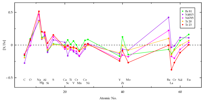
Figure 8: Tr 23 and previously analyzed GES OC abundances vs. atomic number. All abundance ratios are taken from iDR4 analyses and normalized to Grevesse et al. (2007) solar abundances.

7.1 Light elements

We find cluster averages for carbon and oxygen of –0.15 $\pm$ 0.09 dex and +0.08 $\pm$ 0.07 dex respectively. Tautvaišienė et al. (2010) find roughly solar [O/Fe] ratios, and consistent [C/Fe] ratios of $\sim$ -0.2 dex, for Galactic clump stars. The [Fe/H] and [C/Fe] abundances determined by GES for intermediate-age OC Trumpler 20 (Tautvaišienė et al. 2015) at +0.10 and –0.20 dex are similar to those we find for Tr 23; abundances for NGC 4815 and NGC 6705, two clusters closer in age to Tr 23, have solar [Fe/H] abundances but also show subsolar [C/Fe] ratios of –0.16 and –0.08 dex, respectively. All three of these clusters fall at similar Galactocentric radii as Tr 23. As shown in Tautvaišienė et al. (2015), models from Magrini et al. (2009) and Romano et al. (2010) predict solar or slightly subsolar [O/Fe] abundances for an R_GC = 6 kpc, although GES measurements for NGC 4815 and NGC 6705 [O/Fe] are +0.13 dex (Tr 20 stars could not be measured due to telluric contamination of the O feature). Unlike C, stellar evolution models predict that O abundances of evolved stars are primordial. The Tr 23 dispersion in [C/Fe] is slightly larger than [O/Fe], although as with Na we do not expect to observe any significant dispersion in the carbon abundance from clump stars alone.
Tr 23 is significantly enhanced in sodium, with an average measured [Na/Fe] = +0.52 $\pm$ 0.09 dex. We calculate NLTE corrections following Smiljanic et al. (2016) and find a typical correction $<$Na_NLTE – Na${}_{\mathrm{LTE}}>$ = –0.10 dex for Tr 23 clump stars, and a cluster average [Na/Fe]_NLTE of +0.42 $\pm$ 0.08 dex. Smiljanic et al. (2016) also study Na abundances for field dwarfs and giants and find that giant abundances are systematically higher than dwarf abundances for a range of metallicities. Some mixing of products of the NeNa cycle is expected during the first dredge-up stage (El Eid & Champagne 1995), so Na increases in giants may be a real result of stellar evolution, or partly real and partly due to systematic effects. Models of [Na/Fe] for different stellar TO masses from Lagarde et al. (2012) predict an NLTE [Na/Fe] of +0.3 for solar [Fe/H] stars at M_TO = 3M_⊙, including the effects of stellar rotation. [Na/Fe] abundances for other GES OCs seem to match the model predictions, including the youngest of the selected GES clusters, NGC 6705, at 0.3 Gyr and [Na/Fe]_NLTE = 0.38 $\pm$ 0.11. The Tr 23 [Na/Fe] abundance is higher than the Lagarde et al. (2012) rotational mixing models predict for its turnoff mass (M_TO = 2.1M_⊙; see Table 4), but it falls within the giant field star and OC distributions in Smiljanic et al. (2016) and follows the same general trend of increasing [Na/Fe] abundance with increasing TO mass.
We find an [Al/Fe] abundance of +0.20 $\pm$ 0.05 dex; compared to OC aluminum abundances in Smiljanic et al. (2016), which are based on a solar $\epsilon$(Al) = 6.44, the Tr 23 average is typical for solar-metallicity field giants, though it is on the upper edge of the dwarf star distributions in Smiljanic et al. (2016) and Bensby et al. (2014). Once the typical NLTE correction for giants from Smiljanic et al. (2016) of -0.05 dex is applied, the cluster average on that scale becomes +0.08 dex, supporting their finding that OC giants are not enhanced in [Al/Fe] relative to model predictions of Lagarde et al. (2012).

7.2 $\alpha$-elements

Tr 23 has roughly solar [$\alpha$/Fe] ratios for all elements except magnesium. We find an enhanced [Mg/Fe] = +0.20 $\pm$ 0.07, inconsistent with the cluster [Si/Fe], [Ca/Fe] and [Ti/Fe] of 0.03 $\pm$ 0.05, –0.04 $\pm$ 0.03, and –0.04 $\pm$ 0.04, respectively. Previous GES abundance studies have also found enhanced [Mg/Fe] in OCs (see Magrini et al. 2014) compared to other $\alpha$-elements by about 0.2 dex. We note that three Mg lines at $\sim$6300$\mathrm{\AA}$ which are commonly measured via equivalent widths may be affected by a Ca autoionization feature that increases the measured abundances by about 0.2 dex in solar metallicity red giants (Overbeek et al. 2015). However, Magrini et al. (2015) note that O and Mg are almost entirely produced in type II supernovae while Si, Ca, and Ti can have considerable contributions (50 to 70%) from SN Ia; Tr 23 abundances for these two groups are consistent with each other within errors.
$\alpha$-element measurements for the three previously mentioned inner disk GES OCs were presented in Magrini et al. (2014); they find solar or slightly subsolar [Si/Fe], [Ca/Fe], and [Ti/Fe] abundances consistent with solar metallicity field stars of the inner disk and bulge. Cepheid data from Andrievsky et al. (2002) also indicate that [$\alpha$/Fe] ratios in the inner disk are roughly solar and show little relationship with R_GC.

7.3 Fe peak elements

Sc, V, Cr, Mn, Co, and Ni ratios to Fe are all roughly solar. The inner disk clusters also show little variation in these abundances.

7.4 Neutron-capture elements

Y, Zr, Mo, Ba, La, and Ce are majority slow neutron-capture (s-process) elements. There are multiple nucleosynthesis pathways for s-process elements (see, e.g., Travaglio et al. 2004), but AGB stars are thought to be the most significant contributors for young clusters. There is a continuing debate about the size of the contribution from AGB stars; supersolar abundances measured in young OCs for some elements, primarily Ba, suggest that the role of low-mass AGB stars is larger than once thought (D’Orazi et al. 2009; Maiorca et al. 2011; Mishenina et al. 2015). However, other s-process elements do not always show the same enhancement. Jacobson & Friel (2013) measured [Zr/Fe] and [La/Fe] abundances in a sample of 19 OCs and found that the scatter in cluster abundance, particularly for ages $<$ 3 Gyr, is larger than the magnitude of the trends in these elements with age.
OCs younger than 3 Gyr are generally found to have solar or supersolar s-process abundances (Maiorca et al. 2011); Tr 23, however, is subsolar in all measured s-process elements except Ba. We may further subdivide s-process elements into light (Y, Zr, Mo) and heavy (Ba, La, Ce); each of these groups should have very similar abundances. The neutron flux inside AGB stars, as well as the metallicity (i.e., the number of Fe ’seeds’ for neutrons to build on), may affect the relative abundances of the light vs. heavy elements, but the abundances of nuclei of similar atomic weight should strongly correlate. We plot GES cluster averages for neutron-capture elements with age along with literature data from Maiorca et al. (2011) (Y, Zr, La, and Ce), D’Orazi et al. (2009) (Ba), and Overbeek et al. (2016) (Mo, Nd, and Eu) in Figure 9. Colors for GES OCs in Figure 9 are the same as Figure 8 except that M67 is marked in blue (the M67 average is based on giant stars only). The error bars in Figure 9 represent the standard deviations of stellar abundances; the errors on mean cluster abundances are sometimes smaller than the points, particularly for Tr 20 (42 member stars) and N6705 (27 member stars). All literature abundances have been placed on the solar abundance scale of Grevesse et al. (2007). We see in Figure 9 that the GES clusters, and particularly Tr 23, have lower s-process abundances than literature clusters of the same ages. If we look specifically at M67, which is represented in Figure 9 in the literature sample as well as the GES sample (at 4.3 Gyr), we see systematic offsets between the GES and literature abundances, particularly for the light s-process elements. The GES M67 abundances are lower than found by Maiorca et al. (2011) and Overbeek et al. (2016) by 0.1 to 0.2 dex for the light s-process elements, and if we consider these as indicative of systematic offsets between the GES and literature abundance scales, the GES clusters are not significantly lower in light s-process elements than literature clusters of the same ages. However, the M67 heavy s-process element abundances of the two samples agree well, and the younger GES OCs have lower average abundances than literature clusters in their age group. Tr 23 in particular falls below the range of literature abundances for Ba, La, and Ce. We also see a suggestion of large [Ba/Fe] increases ($\sim$0.4 dex) for the youngest two GES clusters (N4815 and N6705) relative to the older clusters, which is not reflected in La or Ce abundances, or the light s-process elements.
In Figure 10 we plot the same GES and literature data against Galactocentric radius using the same colors and abundance error bars as in Figure 9, but with point types marking different age groups; filled circles are clusters $\leq$ 1 Gyr old, crosses are clusters between 1 and 5 Gyr, and open circles are clusters older than 5 Gyr. Looking at all age groups together, we see no clear sign of a relationship between [s-/Fe] abundances and Galactocentric radius. The literature [Zr/Fe] and [La/Fe] samples are not large enough for definite interpretation, but when the systematic differences between M67 values are taken into account, the inner disk (GES) clusters are at the same [Y/Fe], [Mo/Fe], and [Ce/Fe] abundances as literature clusters in the solar neighborhood. [Ba/Fe] shows suggestions of a decrease in the inner disk based on the GES cluster abundances, but in the larger D’Orazi et al. (2009) sample there is considerable scatter around the solar neighborhood, so more data points would be needed in the inner disk to confirm the decrease. When looking at the individual age groups, other than Ba abundances in young OCs there does not seem to be much of a gradient in the light or heavy s-process elements for any of the three age bins.
Nd is a mixed r- and s-process element, and Eu is a majority r-process element, with 42 and 98% solar abundance formed via the r-process, respectively (Sneden et al. 2008). r-process elements are formed in high neutron flux environments, most likely type II supernovae or neutron star mergers. Because these involve different mass ranges of stars than the s-process we necessarily expect relationships of r-process element abundances with cluster age to be different than for the s-process. For Tr 23, we find a solar [Eu/Fe] ratio of 0.00 $\pm$ 0.08 dex and slightly subsolar [Nd/Fe] of -0.12 $\pm$ 0.16. These are similar to the other GES OC abundances in Figure 8, although Tr23 still has the lowest abundances for both elements. In Figure 9 we see that the Tr 23 [Nd/Fe] abundance is within the literature OC distribution although it is on the low end; the other GES clusters match the literature Nd distribution well. The [Eu/Fe] abundances for Tr 23 and the other GES OCs are higher than literature abundances, but if we correct for the apparent offset in measured M67 Eu abundances, the GES OCs are only slightly enhanced in Eu relative to the literature abundances for young clusters.
In Figure 10, [Nd/Fe] does seem to increase with Galactocentric radius, largely due to clusters more than 14 kpc from the Galactic center and especially Be 31 (at 16 kpc) which is based on a single star displaying unusual abundance patterns (Overbeek et al. 2016; Yong et al. 2005). For [Eu/Fe], the intermediate age clusters do show some increase with R_GC; the youngest clusters do not appear to have a gradient, but they also do not probe the outer regions of the disk (beyond 13 kpc) where we see significant increases for older clusters.
It would seem from these data that the inner disk clusters are modestly enhanced in Eu and significantly deficient in heavy s-process element abundances relative to other OCs of similar ages. The scatter in the inner disk clusters, however, is similar to scatter in young clusters in the literature for both r- and s-process elements. The scatter observed in neutron-capture abundances among the GES OCs of similar ages and similar Galactocentric radii (Br 81, N4815, N6705, and Tr 23 are all younger than 1 Gyr and within 7 kpc of the Galactic center) is significant given the small errors on the means; this scatter may be due to localized abundance inhomogeneities in the interstellar medium (ISM). Maiorca et al. (2012) model s-process yields for AGB stars of different masses and different mass C¹³ pockets (the primary source of neutrons in low-mass AGB stars) and show that moderately metal-poor AGB stars of 2 M_⊙ overproduce light s-process elements relative to heavy s-process elements, whereas a star of 1.5 M_⊙ with a larger C¹³ pocket would produce higher yields of heavy s-process elements than light s-process elements. They further note that the factors determining the size of the C¹³ pocket in low-mass stars are not well understood or constrained by observations; it may be that the gas from which Tr 23 formed was preferentially enriched by higher-mass AGB stars which left it deficient in heavy s-process elements, although we would typically expect the inner disk to have old enough stellar populations so that very low-mass AGB stars could have already enriched the ISM. It is also possible that different low-mass AGB stars might have different C¹³ pocket masses (the physical factors driving the pocket mass are unclear so there could be some variation) and produce the light and heavy s-process elements with different efficiencies.
Radial migration may also play a role in moderating any existing gradients and increasing scatter at different Galactocentric radii and ages. Most clusters, however, are not expected to move more than a few kpc and likely occur primarily in the outer disk (Bird et al. 2012), so this cannot be the sole explanation for the behavior of heavy s-process elements in Tr 23.

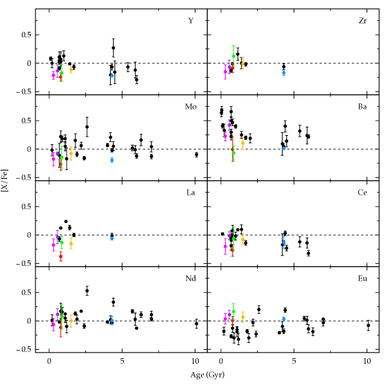
Figure 9: Tr 23 [X/Fe] abundances vs. age in red and M67 abundances in blue compared to literature OC abundances from D’Orazi et al. (2009); Maiorca et al. (2011); Overbeek et al. (2016) in black and other GES OCs the same colors as Figure 8.

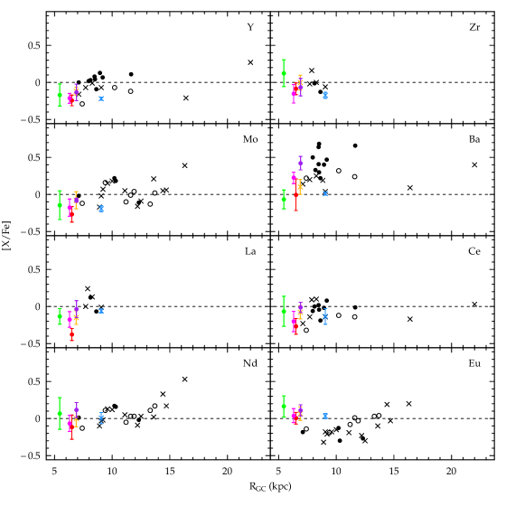
Figure 10: Tr 23 [X/Fe] abundances vs. Galactocentric radius; colors are the same as in Figure 9. Filled circles are clusters $<$ 1 Gyr old, crosses are clusters 2 to 5 Gyr old, and open circles are clusters $>$ 5 Gyr old.

8 Summary and conclusions

The Gaia-ESO Survey has provided the first spectroscopy of the inner disk open cluster Trumpler 23, which has only two existing photometry studies (Carraro et al. 2006; Bonatto & Bica 2007) – it is only 20 pc above the plane of the Galaxy. We use Gaia-ESO radial velocity measurements to find a cluster systemic radial velocity of -61.3 $\pm$ 1.9 km s^-1 (s.d.), and isolate 70 stars out of 167 observed as radial velocity members. We are also able to use GES atmospheric parameters to remove a field star present in the selected cluster radial velocity distribution. Based on our radial velocity membership criteria, we derive an [Fe/H] of +0.14 $\pm$ 0.03 consistent with other OCs in this area of the disk.
Using only stars we have selected as radial velocity members, we re-determine cluster parameters by fitting PARSEC, BaSTI, and Dartmouth isochrones to $V$, $V-I$ photometry from Carraro et al. (2006). With these three sets of model isochrones, we derive ages from 0.60 to 0.80 Gyr, E($V-I$) from 1.02 to 1.10, and distance moduli from 14.15 to 14.50. We adopt the PARSEC isochrone parameters of 0.80 $\pm$ 0.10 Gyr, E($V-I$) = 1.02${}^{+0.14}_{-0.09}$ (E($B-V$) = 0.82${}^{+0.11}_{-0.08}$), and (m$-$M)_V = 14.15 $\pm$ 0.20 (d = 2.10 $\pm$ 0.20, R_GC = 6.30). Our cluster parameters agree within the errors with determinations from both previous photometry studies except for the Bonatto & Bica (2007) E($B-V$) which is substantially lower than ours at 0.58 $\pm$ 0.03. However, the Bonatto & Bica (2007) reddening is based on isochrone fitting to 2MASS $J,H,K$ photometry, and the color relations used may be the source of the discrepancy. We find an apparent spread in the lower MS which is likely due to broadening from both DR and binaries.
We also present ten member star abundances for 23 elements plus iron, based on high-resolution UVES spectra. We find that the cluster has an approximately solar [$\alpha$/Fe] ratio, though with enhanced [Mg/Fe]. It also has an unusually high [Na/Fe] of 0.42 $\pm$ 0.08 which is not seen in other intermediate-age inner disk open clusters analyzed by GES; it does however generally agree with previous findings of increasing [Na/Fe] abundances with increasing cluster turn-off mass. [C/Fe] and [O/Fe] abundances are typical of open clusters; because our high-resolution data was taken for clump stars only we cannot examine changes in C or Na with evolutionary state, and we find no evidence of internal spread in the cluster for any elements. Tr 23 has a solar r-process ratio (as measured by Eu) but appears to be deficient in s-process elements, particularly La, Ce, and Ba; this may be due in part to radial migration, localized enrichment of the ISM, or varying efficiencies of neutron sources in AGB stars.

Table 1: Parameters for Trumpler 23 Radial Velocity Members with GIRAFFE Data

IDa	GES ID	$V^{a}$	$V-I^{a}$	RA	Dec.	Teff	log(g)	$\xi$	[Fe/H]	Vr
		(mag)	(mag)	(deg.)	(deg.)	(K)	(cm s-2)	(km s-1)	(dex)	(km s-1)
18	16005705-5333242	13.950	2.179	240.23771	-53.55672	5501 $\pm$ 150	4.42 $\pm$ 0.02	1.12 $\pm$ 0.02	0.65 $\pm$ 0.29	-62.86 $\pm$ 0.10
19	16004034-5333240	13.938	2.271	240.16808	-53.55667	$\ldots$	$\ldots$	$\ldots$	$\ldots$	-61.17 $\pm$ 0.10
42	16005086-5332030	14.229	1.673	240.21192	-53.53417	6063 $\pm$ 145	3.17 $\pm$ 0.03	1.58 $\pm$ 0.05	$\ldots$	-62.63 $\pm$ 0.10
49	16003972-5331217	14.277	1.607	240.16550	-53.52269	$\ldots$	$\ldots$	$\ldots$	$\ldots$	-59.64 $\pm$ 0.13
112	16004929-5331023	14.717	1.352	240.20538	-53.51731	$\ldots$	$\ldots$	$\ldots$	$\ldots$	-62.53 $\pm$ 0.16
141	16005986-5329431	14.889	1.207	240.24942	-53.49531	$\ldots$	$\ldots$	$\ldots$	$\ldots$	-62.43 $\pm$ 0.18
149	16010227-5333466	15.013	1.329	240.25946	-53.56294	$\ldots$	$\ldots$	$\ldots$	$\ldots$	-64.65 $\pm$ 1.27
165	16004809-5332301	15.123	1.251	240.20038	-53.54169	$\ldots$	$\ldots$	$\ldots$	$\ldots$	-64.21 $\pm$ 0.11
172	16005462-5330451	14.998	1.234	240.22758	-53.51253	$\ldots$	$\ldots$	$\ldots$	$\ldots$	-62.72 $\pm$ 0.21
179	16004639-5333149	15.263	1.259	240.19329	-53.55414	$\ldots$	$\ldots$	$\ldots$	$\ldots$	-62.81 $\pm$ 0.51
197	16005412-5336140	15.735	2.141	240.22550	-53.60389	$\ldots$	$\ldots$	$\ldots$	$\ldots$	-64.29 $\pm$ 0.11
199	16010556-5333133	15.245	1.208	240.27317	-53.55369	$\ldots$	$\ldots$	$\ldots$	$\ldots$	-60.00 $\pm$ 0.50
246	16004693-5334523	15.460	1.210	240.19554	-53.58119	$\ldots$	$\ldots$	$\ldots$	$\ldots$	-64.70 $\pm$ 0.32
254	16010935-5332003	15.410	1.196	240.28896	-53.53342	$\ldots$	$\ldots$	$\ldots$	$\ldots$	-61.79 $\pm$ 0.68
257	16004424-5332421	15.552	1.360	240.18433	-53.54503	7530 $\pm$ 44	$\ldots$	$\ldots$	$\ldots$	-60.12 $\pm$ 0.25
260	16004496-5333060	15.567	1.378	240.18733	-53.55167	$\ldots$	$\ldots$	$\ldots$	$\ldots$	-63.87 $\pm$ 1.72
286	16005715-5332459	15.654	1.361	240.23812	-53.54608	$\ldots$	$\ldots$	$\ldots$	$\ldots$	-57.42 $\pm$ 2.13
297	16005224-5331009	15.647	1.328	240.21767	-53.51692	7755 $\pm$ 52	$\ldots$	$\ldots$	$\ldots$	-63.40 $\pm$ 0.45
301	16004889-5331273	15.717	1.335	240.20371	-53.52425	7621 $\pm$ 54	$\ldots$	$\ldots$	$\ldots$	-60.65 $\pm$ 0.34
312	16005370-5333549	15.679	1.210	240.22375	-53.56525	7924 $\pm$ 63	$\ldots$	$\ldots$	$\ldots$	-62.62 $\pm$ 0.42
319	16003077-5331541	15.860	1.412	240.12821	-53.53169	6039 $\pm$ 83	4.05 $\pm$ 0.26	$\ldots$	0.04 $\pm$ 0.20	-58.00 $\pm$ 0.24
320	16005689-5332277	15.860	1.364	240.23704	-53.54103	$\ldots$	$\ldots$	$\ldots$	$\ldots$	-61.01 $\pm$ 1.22
379	16010382-5331502	15.855	1.258	240.26592	-53.53061	7987 $\pm$ 60	$\ldots$	$\ldots$	$\ldots$	-59.56 $\pm$ 0.25
386	16005638-5333098	15.926	1.238	240.23492	-53.55272	7852 $\pm$ 61	$\ldots$	$\ldots$	$\ldots$	-63.87 $\pm$ 0.49
391	16004787-5334169	15.952	1.219	240.19946	-53.57136	$\ldots$	$\ldots$	$\ldots$	$\ldots$	-59.38 $\pm$ 2.02
392	16005131-5333440	16.016	1.403	240.21379	-53.56222	$\ldots$	$\ldots$	$\ldots$	$\ldots$	-58.80 $\pm$ 0.48
393	16003266-5329243	15.964	1.222	240.13608	-53.49008	$\ldots$	$\ldots$	$\ldots$	$\ldots$	-61.24 $\pm$ 1.94
401	16004946-5329113	15.937	1.268	240.20608	-53.48647	$\ldots$	$\ldots$	$\ldots$	$\ldots$	-57.41 $\pm$ 7.53
406	16004295-5330566	16.153	1.344	240.17896	-53.51572	$\ldots$	$\ldots$	$\ldots$	$\ldots$	-60.35 $\pm$ 2.04
413	16010069-5329384	16.040	1.288	240.25287	-53.49400	$\ldots$	$\ldots$	$\ldots$	$\ldots$	-61.17 $\pm$ 4.45
419	16005951-5335225	16.151	1.337	240.24796	-53.58958	$\ldots$	$\ldots$	$\ldots$	$\ldots$	-62.60 $\pm$ 3.36
429	16004544-5333062	16.146	1.292	240.18933	-53.55172	$\ldots$	$\ldots$	$\ldots$	$\ldots$	-61.19 $\pm$ 3.68
478	16010204-5332060	16.232	1.352	240.25850	-53.53500	$\ldots$	$\ldots$	$\ldots$	$\ldots$	-62.07 $\pm$ 2.28
484	16005062-5331383	16.208	1.228	240.21092	-53.52731	$\ldots$	$\ldots$	$\ldots$	$\ldots$	-62.26 $\pm$ 0.39
489	16010489-5329440	16.270	1.347	240.27038	-53.49556	$\ldots$	$\ldots$	$\ldots$	$\ldots$	-61.10 $\pm$ 0.53
496	16010476-5328190	16.273	1.389	240.26983	-53.47194	$\ldots$	$\ldots$	$\ldots$	$\ldots$	-62.97 $\pm$ 1.91
501	16010497-5333409	16.240	1.220	240.27071	-53.56136	8177 $\pm$ 82	$\ldots$	$\ldots$	$\ldots$	-61.24 $\pm$ 0.32
509	16004168-5332182	16.393	1.311	240.17367	-53.53839	$\ldots$	$\ldots$	$\ldots$	$\ldots$	-62.82 $\pm$ 0.53
531	16005584-5328374	16.480	1.441	240.23267	-53.47706	7712 $\pm$ 79	$\ldots$	$\ldots$	$\ldots$	-58.26 $\pm$ 0.76
556	16010454-5328438	16.387	1.254	240.26892	-53.47883	$\ldots$	$\ldots$	$\ldots$	$\ldots$	-61.19 $\pm$ 0.86
576	16005741-5335518	16.547	1.392	240.23921	-53.59772	8021 $\pm$ 84	$\ldots$	$\ldots$	$\ldots$	-57.85 $\pm$ 0.50
579	16010723-5333561	16.485	1.217	240.28012	-53.56558	7582 $\pm$ 82	$\ldots$	$\ldots$	$\ldots$	-60.58 $\pm$ 0.46
623	16010108-5331400	16.550	1.335	240.25450	-53.52778	7604 $\pm$ 249	4.18 $\pm$ 0.15	$\ldots$	0.02 $\pm$ 0.20	-60.06 $\pm$ 0.46
634	16005175-5332339	16.682	1.471	240.21562	-53.54275	7306 $\pm$ 783	4.15 $\pm$ 0.18	$\ldots$	-0.07 $\pm$ 0.46	-64.20 $\pm$ 0.57
792	16005774-5334375	16.915	1.369	240.24058	-53.57708	6812 $\pm$ 307	4.06 $\pm$ 0.19	$\ldots$	0.19 $\pm$ 0.30	-59.04 $\pm$ 0.58
815	16004357-5328513	17.005	1.514	240.18154	-53.48092	6722 $\pm$ 435	4.13 $\pm$ 0.02	$\ldots$	0.32 $\pm$ 0.35	-62.09 $\pm$ 0.53
821	16004569-5332567	17.063	1.497	240.19037	-53.54908	7058 $\pm$ 488	4.15 $\pm$ 0.21	$\ldots$	0.11 $\pm$ 0.15	-64.93 $\pm$ 0.66
877	16004906-5330204	17.137	1.436	240.20442	-53.50567	6809 $\pm$ 344	4.13 $\pm$ 0.19	$\ldots$	0.25 $\pm$ 0.36	-58.10 $\pm$ 0.97
922	16005585-5335245	17.148	1.403	240.23271	-53.59014	7062 $\pm$ 553	4.10 $\pm$ 0.19	$\ldots$	-0.07 $\pm$ 0.46	-61.26 $\pm$ 0.70
981	16004581-5331557	17.266	1.476	240.19088	-53.53214	6766 $\pm$ 407	4.46 $\pm$ 0.36	$\ldots$	0.20 $\pm$ 0.40	-64.23 $\pm$ 0.98
1004	16005827-5330323	17.325	1.449	240.24279	-53.50897	7055 $\pm$ 666	4.05 $\pm$ 0.23	$\ldots$	0.12 $\pm$ 0.14	-60.44 $\pm$ 0.36
1012	16010533-5333195	17.311	1.535	240.27221	-53.55542	6378 $\pm$ 181	4.32 $\pm$ 0.27	$\ldots$	0.17 $\pm$ 0.18	-60.91 $\pm$ 0.32
1016	16004350-5331482	17.327	1.429	240.18125	-53.53006	6584 $\pm$ 440	4.05 $\pm$ 0.21	$\ldots$	0.30 $\pm$ 0.42	-60.13 $\pm$ 1.01
1061	16004174-5333545	17.432	1.555	240.17392	-53.56514	6406 $\pm$ 186	4.24 $\pm$ 0.32	$\ldots$	0.06 $\pm$ 0.15	-58.33 $\pm$ 0.29
1355	16005469-5334324	17.828	1.647	240.22788	-53.57567	5993 $\pm$ 156	4.18 $\pm$ 0.42	$\ldots$	-0.02 $\pm$ 0.21	-57.32 $\pm$ 0.32
1358	16005146-5332497	17.773	1.538	240.21442	-53.54714	6517 $\pm$ 397	3.90 $\pm$ 0.16	$\ldots$	0.27 $\pm$ 0.28	-60.99 $\pm$ 1.09
1436	16003891-5330304	17.913	1.629	240.16213	-53.50844	6364 $\pm$ 181	4.64 $\pm$ 0.83	$\ldots$	0.25 $\pm$ 0.20	-60.30 $\pm$ 0.77
1483	16005675-5335029	17.896	1.560	240.23646	-53.58414	6527 $\pm$ 203	4.36 $\pm$ 0.43	$\ldots$	0.25 $\pm$ 0.25	-60.39 $\pm$ 0.45
1491	16010323-5330273	17.938	1.556	240.26346	-53.50758	6647 $\pm$ 492	4.05 $\pm$ 0.12	$\ldots$	0.39 $\pm$ 0.43	-61.07 $\pm$ 0.36
1528	16005241-5331345	17.940	1.567	240.21838	-53.52625	6602 $\pm$ 414	4.07 $\pm$ 0.19	$\ldots$	0.27 $\pm$ 0.38	-63.36 $\pm$ 0.61

Table 2: Parameters for Trumpler 23 Radial Velocity Non-members with GIRAFFE Data

IDa	GES ID	$V^{a}$	$V-I^{a}$	RA	Dec.	Teff	log(g)	$\xi$	[Fe/H]	Vr
		(mag)	(mag)	(deg.)	(deg.)	(K)	(cm s-2)	(km s-1)	(dex)	(km s-1)
36	16005835-5329550	13.553	0.988	240.24312	-53.49861	$\ldots$	$\ldots$	$\ldots$	$\ldots$	-54.36 $\pm$ 0.11
39	16004521-5332044	13.938	1.249	240.18838	-53.53456	$\ldots$	$\ldots$	$\ldots$	$\ldots$	-132.95 $\pm$ 0.10
71	16004917-5333257	14.151	0.998	240.20487	-53.55714	$\ldots$	$\ldots$	$\ldots$	$\ldots$	41.98 $\pm$ 0.61
73	16004353-5330424	14.210	1.132	240.18138	-53.51178	$\ldots$	$\ldots$	$\ldots$	$\ldots$	-10.06 $\pm$ 0.10
80	16005170-5333015	14.133	0.889	240.21542	-53.55042	$\ldots$	$\ldots$	$\ldots$	$\ldots$	-20.20 $\pm$ 0.11
104	16003549-5331214	14.552	1.026	240.14787	-53.52261	$\ldots$	$\ldots$	$\ldots$	$\ldots$	-38.57 $\pm$ 0.50
129	16003881-5331400	14.806	1.253	240.16171	-53.52778	$\ldots$	$\ldots$	$\ldots$	$\ldots$	-38.33 $\pm$ 0.11
135	16004252-5330337	14.568	0.921	240.17717	-53.50936	$\ldots$	$\ldots$	$\ldots$	$\ldots$	-32.38 $\pm$ 0.54
145	16010286-5328087	15.213	1.674	240.26192	-53.46908	$\ldots$	$\ldots$	$\ldots$	$\ldots$	-32.90 $\pm$ 0.17
146	16003985-5333514	14.988	1.259	240.16604	-53.56428	$\ldots$	$\ldots$	$\ldots$	$\ldots$	-55.06 $\pm$ 0.10
183	16005980-5334552	15.188	1.033	240.24917	-53.58200	$\ldots$	$\ldots$	$\ldots$	$\ldots$	-38.10 $\pm$ 2.32
189	16005475-5335022	15.400	1.576	240.22813	-53.58394	$\ldots$	$\ldots$	$\ldots$	$\ldots$	78.38 $\pm$ 0.14
191	16003979-5329242	15.183	1.191	240.16579	-53.49006	5083 $\pm$ 93	4.55 $\pm$ 0.04	0.74 $\pm$ 0.04	0.18 $\pm$ 0.14	-31.70 $\pm$ 0.10
208	16005846-5335490	15.342	1.314	240.24358	-53.59694	$\ldots$	$\ldots$	$\ldots$	$\ldots$	-55.99 $\pm$ 1.56
209	16005739-5332261	15.225	1.208	240.23913	-53.54058	$\ldots$	$\ldots$	$\ldots$	$\ldots$	-68.80 $\pm$ 0.14
212	16010451-5332442	15.240	1.204	240.26879	-53.54561	$\ldots$	$\ldots$	$\ldots$	$\ldots$	-50.19 $\pm$ 0.10
213	16005402-5331231	15.721	1.944	240.22508	-53.52308	5257 $\pm$ 108	3.16 $\pm$ 0.05	1.41 $\pm$ 0.03	-0.10 $\pm$ 0.24	13.86 $\pm$ 0.12
214	16004351-5333456	15.403	1.418	240.18129	-53.56267	$\ldots$	$\ldots$	$\ldots$	$\ldots$	-31.21 $\pm$ 0.10
216	16004226-5335450	15.356	1.243	240.17608	-53.59583	$\ldots$	$\ldots$	$\ldots$	$\ldots$	-68.53 $\pm$ 2.95
217	16003389-5330469	15.449	1.248	240.14121	-53.51303	$\ldots$	$\ldots$	$\ldots$	$\ldots$	-48.00 $\pm$ 1.70
219	16010922-5330561	14.936	1.035	240.28842	-53.51558	$\ldots$	$\ldots$	$\ldots$	$\ldots$	-21.27 $\pm$ 3.42
222	16005026-5333580	15.377	1.306	240.20942	-53.56611	$\ldots$	$\ldots$	$\ldots$	$\ldots$	-3.47 $\pm$ 1.08
225	16010322-5332285	15.431	1.437	240.26342	-53.54125	$\ldots$	$\ldots$	$\ldots$	$\ldots$	-51.04 $\pm$ 1.60
226	16010444-5330031	15.351	1.302	240.26850	-53.50086	$\ldots$	$\ldots$	$\ldots$	$\ldots$	-68.84 $\pm$ 2.72
247	16004890-5328089	15.524	1.430	240.20375	-53.46914	$\ldots$	$\ldots$	$\ldots$	$\ldots$	-16.31 $\pm$ 0.16
252	16010967-5332235	15.573	1.476	240.29029	-53.53986	$\ldots$	$\ldots$	$\ldots$	$\ldots$	-55.20 $\pm$ 0.10
255	16003791-5331140	15.552	1.056	240.15796	-53.52056	$\ldots$	$\ldots$	$\ldots$	$\ldots$	-44.08 $\pm$ 3.49
261	16004556-5332159	15.611	1.393	240.18983	-53.53775	4542 $\pm$ 144	4.61 $\pm$ 0.43	$\ldots$	0.15 $\pm$ 0.16	-24.98 $\pm$ 0.24
262	16010496-5332496	15.541	1.331	240.27067	-53.54711	6614 $\pm$ 305	4.15 $\pm$ 0.23	$\ldots$	-0.04 $\pm$ 0.19	7.52 $\pm$ 0.24
276	16005205-5335459	15.598	1.257	240.21687	-53.59608	$\ldots$	$\ldots$	$\ldots$	$\ldots$	-35.45 $\pm$ 0.25
279	16004926-5333097	15.545	1.183	240.20525	-53.55269	$\ldots$	$\ldots$	$\ldots$	$\ldots$	-91.20 $\pm$ 0.15
303	16010676-5333432	15.714	1.328	240.27817	-53.56200	$\ldots$	$\ldots$	$\ldots$	$\ldots$	-37.55 $\pm$ 1.11
304	16004058-5329583	15.734	1.385	240.16908	-53.49953	$\ldots$	$\ldots$	$\ldots$	$\ldots$	-66.25 $\pm$ 0.11
314	16003652-5330052	15.699	1.223	240.15217	-53.50144	$\ldots$	$\ldots$	$\ldots$	$\ldots$	-80.31 $\pm$ 0.10
315	16003754-5333550	15.724	1.274	240.15642	-53.56528	7582 $\pm$ 48	$\ldots$	$\ldots$	$\ldots$	-31.20 $\pm$ 0.41
331	16003799-5334228	15.874	1.409	240.15829	-53.57300	6569 $\pm$ 39	4.46 $\pm$ 0.08	$\ldots$	0.45 $\pm$ 0.03	-4.58 $\pm$ 0.33
344	16004804-5333020	15.849	1.386	240.20017	-53.55056	$\ldots$	$\ldots$	$\ldots$	$\ldots$	-14.73 $\pm$ 0.24
353	16010155-5328151	15.795	1.191	240.25646	-53.47086	$\ldots$	$\ldots$	$\ldots$	$\ldots$	458.82 $\pm$ 0.10
366	16010826-5331372	15.808	1.243	240.28442	-53.52700	4967 $\pm$ 151	4.56 $\pm$ 0.36	$\ldots$	0.04 $\pm$ 0.14	5.64 $\pm$ 0.24
370	16003334-5329569	15.889	1.124	240.13892	-53.49914	5897 $\pm$ 101	4.16 $\pm$ 0.06	1.17 $\pm$ 0.03	-0.18 $\pm$ 0.15	-28.76 $\pm$ 0.10
373	16004375-5335538	15.970	1.278	240.18229	-53.59828	$\ldots$	$\ldots$	$\ldots$	$\ldots$	-33.92 $\pm$ 0.13
381	16004932-5332384	15.945	1.149	240.20550	-53.54400	5365 $\pm$ 87	4.27 $\pm$ 0.02	1.50 $\pm$ 0.07	0.09 $\pm$ 0.18	-24.87 $\pm$ 0.11
382	16005577-5329141	15.867	1.199	240.23237	-53.48725	$\ldots$	$\ldots$	$\ldots$	$\ldots$	-86.37 $\pm$ 0.12
384	16004196-5335545	16.039	1.273	240.17483	-53.59847	$\ldots$	$\ldots$	$\ldots$	$\ldots$	-25.35 $\pm$ 0.36
446	16010350-5329301	16.023	1.081	240.26458	-53.49169	8034 $\pm$ 67	$\ldots$	$\ldots$	$\ldots$	-45.83 $\pm$ 0.61
464	16005229-5333251	16.178	1.310	240.21787	-53.55697	$\ldots$	$\ldots$	$\ldots$	$\ldots$	-33.96 $\pm$ 0.15
476	16005961-5331283	16.310	1.428	240.24838	-53.52453	$\ldots$	$\ldots$	$\ldots$	$\ldots$	-67.45 $\pm$ 8.35
492	16003558-5329192	16.222	1.183	240.14825	-53.48867	$\ldots$	$\ldots$	$\ldots$	$\ldots$	-75.27 $\pm$ 0.11
494	16005700-5330159	16.400	1.484	240.23750	-53.50442	6535 $\pm$ 54	3.81 $\pm$ 0.11	$\ldots$	0.44 $\pm$ 0.04	-47.43 $\pm$ 0.27
497	16003142-5330137	16.385	1.294	240.13092	-53.50381	6051 $\pm$ 125	4.31 $\pm$ 0.39	$\ldots$	-0.01 $\pm$ 0.25	-35.71 $\pm$ 0.24
499	16005117-5330529	16.336	1.335	240.21321	-53.51469	$\ldots$	$\ldots$	$\ldots$	$\ldots$	-65.98 $\pm$ 1.25
514	16005793-5329383	16.287	1.184	240.24138	-53.49397	5319 $\pm$ 109	4.69 $\pm$ 0.05	1.79 $\pm$ 0.03	-0.19 $\pm$ 0.20	-37.19 $\pm$ 0.12
526	16005684-5329384	16.338	1.302	240.23683	-53.49400	$\ldots$	$\ldots$	$\ldots$	$\ldots$	-22.16 $\pm$ 0.18
530	16010748-5333272	16.347	1.335	240.28117	-53.55756	$\ldots$	$\ldots$	$\ldots$	$\ldots$	-17.90 $\pm$ 3.91
540	16005040-5331031	16.433	1.319	240.21000	-53.51753	$\ldots$	$\ldots$	$\ldots$	$\ldots$	-112.42 $\pm$ 0.75
542	16005288-5331550	16.475	1.458	240.22033	-53.53194	$\ldots$	$\ldots$	$\ldots$	$\ldots$	-12.73 $\pm$ 1.35
543	16005553-5330246	16.316	1.315	240.23138	-53.50683	7410 $\pm$ 74	$\ldots$	$\ldots$	$\ldots$	-4.35 $\pm$ 0.56
560	16003787-5331536	16.561	1.476	240.15779	-53.53156	7080 $\pm$ 718	4.15 $\pm$ 0.21	$\ldots$	0.12 $\pm$ 0.14	-54.37 $\pm$ 0.63
572	16003903-5333026	16.487	1.333	240.16262	-53.55072	$\ldots$	$\ldots$	$\ldots$	$\ldots$	-69.24 $\pm$ 4.01
584	16011001-5331319	16.534	1.449	240.29171	-53.52553	6717 $\pm$ 294	4.00 $\pm$ 0.11	$\ldots$	0.15 $\pm$ 0.32	-29.77 $\pm$ 0.41
585	16005947-5328024	16.519	1.217	240.24779	-53.46733	4933 $\pm$ 166	4.64 $\pm$ 0.20	$\ldots$	0.04 $\pm$ 0.15	10.43 $\pm$ 0.24
591	16004161-5333182	16.486	1.241	240.17337	-53.55506	5188 $\pm$ 51	4.56 $\pm$ 0.34	$\ldots$	0.02 $\pm$ 0.13	42.31 $\pm$ 0.25
621	16005269-5333085	16.576	1.304	240.21954	-53.55236	7556 $\pm$ 80	$\ldots$	$\ldots$	$\ldots$	-66.27 $\pm$ 0.60
651	16004658-5334434	16.222	1.128	240.19408	-53.57872	$\ldots$	$\ldots$	$\ldots$	$\ldots$	-14.61 $\pm$ 0.22
659	16003500-5334335	16.710	1.477	240.14583	-53.57597	6752 $\pm$ 62	4.15 $\pm$ 0.12	$\ldots$	0.45 $\pm$ 0.05	-47.11 $\pm$ 0.64
685	16005470-5334459	16.770	1.361	240.22792	-53.57942	4755 $\pm$ 142	4.66 $\pm$ 0.22	$\ldots$	-0.14 $\pm$ 0.13	48.50 $\pm$ 0.24
709	16004956-5329564	16.808	1.517	240.20650	-53.49900	6189 $\pm$ 124	3.99 $\pm$ 0.19	$\ldots$	0.02 $\pm$ 0.23	-40.43 $\pm$ 0.30
747	16003312-5332533	16.962	1.581	240.13800	-53.54814	6100 $\pm$ 310	4.24 $\pm$ 0.23	$\ldots$	0.30 $\pm$ 0.30	-88.39 $\pm$ 0.25
779	16005584-5333412	16.893	1.300	240.23267	-53.56144	7674 $\pm$ 568	4.17 $\pm$ 0.15	$\ldots$	0.02 $\pm$ 0.20	-49.88 $\pm$ 0.49
787	16004146-5328081	17.063	1.641	240.17275	-53.46892	6509 $\pm$ 263	4.22 $\pm$ 0.40	$\ldots$	0.32 $\pm$ 0.25	-32.88 $\pm$ 0.46
828	16004452-5329038	17.111	1.596	240.18550	-53.48439	6273 $\pm$ 204	4.27 $\pm$ 0.35	$\ldots$	0.08 $\pm$ 0.21	-34.78 $\pm$ 0.26
878	16005429-5329248	17.198	1.596	240.22621	-53.49022	5914 $\pm$ 206	4.04 $\pm$ 0.25	$\ldots$	-0.25 $\pm$ 0.17	-90.02 $\pm$ 0.27
907	16003886-5335108	17.263	1.669	240.16192	-53.58633	8142 $\pm$ 117	$\ldots$	$\ldots$	$\ldots$	-20.97 $\pm$ 0.42
920	16005372-5328100	17.313	1.716	240.22383	-53.46944	6355 $\pm$ 168	3.93 $\pm$ 0.03	$\ldots$	0.20 $\pm$ 0.21	-37.29 $\pm$ 0.26
982	16003991-5335351	17.319	1.523	240.16629	-53.59308	4479 $\pm$ 118	4.79 $\pm$ 0.25	$\ldots$	-0.03 $\pm$ 0.13	48.80 $\pm$ 0.25
990	16005659-5327535	17.349	1.573	240.23579	-53.46486	5794 $\pm$ 73	4.49 $\pm$ 0.19	$\ldots$	-0.21 $\pm$ 0.16	25.82 $\pm$ 0.29
992	16004925-5334087	17.205	1.373	240.20521	-53.56908	6824 $\pm$ 318	4.25 $\pm$ 0.05	$\ldots$	0.29 $\pm$ 0.27	-26.79 $\pm$ 0.38
996	16004583-5330286	17.369	1.603	240.19096	-53.50794	5649 $\pm$ 43	4.29 $\pm$ 0.05	$\ldots$	0.00 $\pm$ 0.15	-0.65 $\pm$ 0.27
1060	16010238-5331368	17.449	1.629	240.25992	-53.52689	6369 $\pm$ 193	4.56 $\pm$ 0.46	$\ldots$	0.29 $\pm$ 0.23	-22.50 $\pm$ 0.42
1088	16004767-5332334	17.543	1.760	240.19862	-53.54261	5497 $\pm$ 114	4.32 $\pm$ 0.10	$\ldots$	-0.08 $\pm$ 0.21	12.24 $\pm$ 0.27
1111	16005412-5328296	17.541	1.712	240.22550	-53.47489	6285 $\pm$ 177	4.27 $\pm$ 0.26	$\ldots$	0.10 $\pm$ 0.14	13.44 $\pm$ 0.31
1112	16005823-5333282	17.465	1.554	240.24263	-53.55783	6253 $\pm$ 389	4.17 $\pm$ 0.39	$\ldots$	0.14 $\pm$ 0.33	-80.74 $\pm$ 0.28
1133	16010614-5329010	17.518	1.607	240.27558	-53.48361	5941 $\pm$ 136	4.26 $\pm$ 0.05	$\ldots$	0.19 $\pm$ 0.12	-11.01 $\pm$ 0.25
1139	16005380-5336063	17.546	1.635	240.22417	-53.60175	5966 $\pm$ 155	4.26 $\pm$ 0.26	$\ldots$	0.02 $\pm$ 0.15	-40.47 $\pm$ 0.27
1183	16005857-5329161	17.582	1.580	240.24404	-53.48781	5882 $\pm$ 115	4.10 $\pm$ 0.15	$\ldots$	0.16 $\pm$ 0.15	-32.19 $\pm$ 0.28
1244	16004689-5328513	17.640	1.516	240.19538	-53.48092	6082 $\pm$ 252	4.37 $\pm$ 0.22	$\ldots$	0.11 $\pm$ 0.21	16.70 $\pm$ 0.27
1416	16003805-5331267	17.828	1.527	240.15854	-53.52408	6325 $\pm$ 602	4.01 $\pm$ 0.19	$\ldots$	0.02 $\pm$ 0.24	-68.03 $\pm$ 1.22
1437	16005817-5334494	17.869	1.556	240.24238	-53.58039	5274 $\pm$ 109	4.71 $\pm$ 0.37	$\ldots$	0.04 $\pm$ 0.12	7.75 $\pm$ 0.27
1466	16004240-5332325	17.976	1.768	240.17667	-53.54236	5890 $\pm$ 169	4.12 $\pm$ 0.18	$\ldots$	0.37 $\pm$ 0.16	-24.58 $\pm$ 0.26
1475	16005947-5330396	17.923	1.635	240.24779	-53.51100	6169 $\pm$ 120	4.63 $\pm$ 0.77	$\ldots$	-0.01 $\pm$ 0.31	-54.25 $\pm$ 0.47
1487	16010669-5328395	17.988	1.740	240.27787	-53.47764	5238 $\pm$ 115	3.99 $\pm$ 0.32	$\ldots$	0.19 $\pm$ 0.29	-123.55 $\pm$ 0.26

Table 3: Parameters for Trumpler 23 Targets with UVES Data

IDa	GES ID	Va	V-Ia	RA	Dec	S/N	RV	Teff	$\log$ g	$\xi$	[Fe/H]	RV Mem.?
		(mag)	(mag)	(deg.)	(deg.)		(km s-1)	(K)	(cm s-2)	(km s-1)	(dex)
52	16005168-5332013	14.644	2.006	240.21533	-53.53369	126	-62.83 $\pm$ 0.57	4881 $\pm$ 117	2.60 $\pm$ 0.23	1.71 $\pm$ 0.16	0.17 $\pm$ 0.10	Y
55	16003935-5332367	14.662	2.039	240.16396	-53.54353	133	-60.94 $\pm$ 0.57	4796 $\pm$ 123	2.57 $\pm$ 0.23	1.47 $\pm$ 0.13	0.14 $\pm$ 0.10	Y
56	16004035-5333047	14.731	2.089	240.16813	-53.55131	125	-68.64 $\pm$ 0.57	4897 $\pm$ 121	3.40 $\pm$ 0.26	1.26 $\pm$ 0.16	0.00 $\pm$ 0.13	N
58	16010433-5332336	14.743	2.017	240.26804	-53.54267	66	-60.53 $\pm$ 0.57	4776 $\pm$ 122	2.48 $\pm$ 0.24	1.68 $\pm$ 0.18	0.17 $\pm$ 0.10	Y
59	16010770-5329374	14.949	2.175	240.28208	-53.49372	124	-61.52 $\pm$ 0.57	4832 $\pm$ 115	2.64 $\pm$ 0.23	1.47 $\pm$ 0.12	0.16 $\pm$ 0.10	Y
64	16005220-5333362	14.721	1.953	240.21750	-53.56006	114	-62.45 $\pm$ 0.57	4917 $\pm$ 116	2.63 $\pm$ 0.22	1.64 $\pm$ 0.13	0.18 $\pm$ 0.10	Y
74	16004569-5329177	14.769	1.867	240.19038	-53.48825	120	-55.40 $\pm$ 0.57	5008 $\pm$ 123	2.98 $\pm$ 0.23	1.45 $\pm$ 0.04	0.18 $\pm$ 0.10	N
86	16004025-5329439	14.992	1.958	240.16771	-53.49553	111	-56.47 $\pm$ 0.57	4912 $\pm$ 125	2.77 $\pm$ 0.24	1.51 $\pm$ 0.14	0.11 $\pm$ 0.10	N
89	16004572-5332095	14.948	2.031	240.19050	-53.53597	84	-43.27 $\pm$ 0.57	4900 $\pm$ 125	2.68 $\pm$ 0.26	1.53 $\pm$ 0.14	0.15 $\pm$ 0.10	N
92	16005798-5331476	15.086	2.077	240.24158	-53.52989	83	-59.95 $\pm$ 0.57	4863 $\pm$ 118	2.69 $\pm$ 0.24	1.46 $\pm$ 0.07	0.13 $\pm$ 0.10	Y
97	16010639-5331056	15.082	2.046	240.27663	-53.51822	56	-61.94 $\pm$ 0.57	4848 $\pm$ 121	2.74 $\pm$ 0.24	1.76 $\pm$ 0.17	0.14 $\pm$ 0.11	Y
105	16010025-5333101	15.138	2.031	240.25104	-53.55281	84	-60.24 $\pm$ 0.57	4884 $\pm$ 119	2.79 $\pm$ 0.22	1.53 $\pm$ 0.25	0.10 $\pm$ 0.10	Y
128	16003885-5334507	15.320	2.148	240.16188	-53.58075	80	-61.15 $\pm$ 0.57	4509 $\pm$ 135	2.42 $\pm$ 0.24	1.49 $\pm$ 0.29	0.08 $\pm$ 0.10	Y
131	16005072-5335536	15.213	1.918	240.21133	-53.59822	50	-8.95 $\pm$ 0.57	4878 $\pm$ 126	2.95 $\pm$ 0.24	1.48 $\pm$ 0.05	0.19 $\pm$ 0.10	N
137	16004312-5330509	15.331	2.046	240.17967	-53.51414	89	-61.79 $\pm$ 0.57	4913 $\pm$ 121	2.86 $\pm$ 0.23	1.60 $\pm$ 0.25	0.11 $\pm$ 0.10	Y
147	16004973-5331459	15.522	2.168	240.20721	-53.52942	72	-10.31 $\pm$ 0.57	4449 $\pm$ 126	2.43 $\pm$ 0.24	1.64 $\pm$ 0.17	0.21 $\pm$ 0.09	N

Table 4: Isochrone Fit Parameters

Model	Age	E(V-I)	E(B-V)	(m-M)V	d⊙	RGC	MTO
	(Gyr)	(mag)	(mag)	(mag)	(kpc)	(kpc)	(M⊙)
PARSEC	0.80 $\pm$ 0.10	1.02${}^{+0.14}_{-0.09}$	0.82${}^{+0.11}_{-0.08}$	14.15 $\pm$ 0.20	2.10 $\pm$ 0.20	6.30 $\pm$ 0.15	2.05
BASTI	0.60 $\pm$ 0.10	1.09${}^{+0.14}_{-0.09}$	0.87${}^{+0.11}_{-0.08}$	14.50 $\pm$ 0.20	2.29 $\pm$ 0.20	6.15 $\pm$ 0.15	2.17
Dartmouth	0.65 $\pm$ 0.10	1.10${}^{+0.14}_{-0.09}$	0.88${}^{+0.11}_{-0.08}$	14.45 $\pm$ 0.20	2.21 $\pm$ 0.20	6.22 $\pm$ 0.15	2.16
Padova (Carraro et al. 2006)	0.60 $\pm$ 0.10	1.05 $\pm$ 0.05	0.84 $\pm$ 0.04	14.35 $\pm$ 0.20	2.23 $\pm$ 0.20	6.20 $\pm$ 0.15	$\ldots$
Padova (Bonatto & Bica 2007)	0.9 $\pm$ 0.1	$\ldots$	0.58 $\pm$ 0.03	13.19 $\pm$ 0.11	1.9 $\pm$ 0.1	6.45 $\pm$ 0.08	$\ldots$

Table 5: UVES Target Light and $\alpha$-Element Abundances

ID	C I	O I	Na I	Mg I	Al I	Si I	S I	Ca I	Ti I
52	8.33 $\pm$ 0.13	8.95 $\pm$ 0.25	6.92 $\pm$ 0.08	7.87 $\pm$ 0.12	6.70 $\pm$ 0.06	7.72 $\pm$ 0.07	7.44 $\pm$ 0.07	6.36 $\pm$ 0.08	4.98 $\pm$ 0.08
55	8.44 $\pm$ 0.13	8.91 $\pm$ 0.14	6.82 $\pm$ 0.06	7.87 $\pm$ 0.12	6.67 $\pm$ 0.07	7.62 $\pm$ 0.07	7.39 $\pm$ 0.07	6.43 $\pm$ 0.09	4.98 $\pm$ 0.08
58	8.45 $\pm$ 0.13	8.80 $\pm$ 0.11	6.78 $\pm$ 0.05	7.91 $\pm$ 0.12	6.70 $\pm$ 0.07	7.60 $\pm$ 0.07	7.35 $\pm$ 0.07	6.36 $\pm$ 0.08	4.95 $\pm$ 0.08
59	8.28 $\pm$ 0.13	8.79 $\pm$ 0.33	6.90 $\pm$ 0.08	7.86 $\pm$ 0.12	6.65 $\pm$ 0.07	7.71 $\pm$ 0.07	7.41 $\pm$ 0.07	6.48 $\pm$ 0.08	5.06 $\pm$ 0.08
64	8.40 $\pm$ 0.13	8.92 $\pm$ 0.23	6.80 $\pm$ 0.06	7.88 $\pm$ 0.12	6.68 $\pm$ 0.07	7.64 $\pm$ 0.07	7.38 $\pm$ 0.07	6.43 $\pm$ 0.08	4.93 $\pm$ 0.09
92	8.34 $\pm$ 0.13	8.81 $\pm$ 0.12	6.85 $\pm$ 0.06	7.82 $\pm$ 0.12	6.65 $\pm$ 0.07	7.66 $\pm$ 0.07	7.42 $\pm$ 0.07	6.36 $\pm$ 0.08	4.92 $\pm$ 0.09
97	8.40 $\pm$ 0.13	8.85 $\pm$ 0.12	6.79 $\pm$ 0.05	7.78 $\pm$ 0.12	6.71 $\pm$ 0.07	7.66 $\pm$ 0.07	7.46 $\pm$ 0.07	6.33 $\pm$ 0.08	4.96 $\pm$ 0.08
105	8.25 $\pm$ 0.13	8.80 $\pm$ 0.12	6.81 $\pm$ 0.05	7.67 $\pm$ 0.12	6.70 $\pm$ 0.06	7.67 $\pm$ 0.07	7.43 $\pm$ 0.07	6.42 $\pm$ 0.08	4.94 $\pm$ 0.08
128	8.47 $\pm$ 0.13	8.84 $\pm$ 0.12	6.61 $\pm$ 0.08	7.95 $\pm$ 0.12	6.71 $\pm$ 0.07	7.63 $\pm$ 0.07	7.45 $\pm$ 0.07	6.36 $\pm$ 0.09	5.02 $\pm$ 0.08
137	8.24 $\pm$ 0.13	8.93 $\pm$ 0.12	6.78 $\pm$ 0.06	7.92 $\pm$ 0.12	6.69 $\pm$ 0.06	7.69 $\pm$ 0.07	7.42 $\pm$ 0.07	6.42 $\pm$ 0.08	5.05 $\pm$ 0.09

Table 6: UVES Target Fe-Peak Abundances

ID	Sc I	V I	Cr I	Mn I	Fe I	Fe II	Co I	Ni I
52	3.24 $\pm$ 0.10	4.09 $\pm$ 0.09	5.72 $\pm$ 0.12	5.46 $\pm$ 0.12	7.57 $\pm$ 0.10	7.66 $\pm$ 0.09	5.05 $\pm$ 0.11	6.38 $\pm$ 0.09
55	3.42 $\pm$ 0.08	4.10 $\pm$ 0.09	5.73 $\pm$ 0.13	5.39 $\pm$ 0.12	7.61 $\pm$ 0.10	7.65 $\pm$ 0.09	5.06 $\pm$ 0.10	6.40 $\pm$ 0.10
58	3.35 $\pm$ 0.08	4.07 $\pm$ 0.08	5.66 $\pm$ 0.10	5.39 $\pm$ 0.11	7.56 $\pm$ 0.10	7.55 $\pm$ 0.09	5.02 $\pm$ 0.10	6.33 $\pm$ 0.10
59	3.36 $\pm$ 0.09	4.15 $\pm$ 0.09	5.78 $\pm$ 0.11	5.36 $\pm$ 0.12	7.63 $\pm$ 0.10	7.70 $\pm$ 0.09	5.10 $\pm$ 0.10	6.44 $\pm$ 0.10
64	3.24 $\pm$ 0.10	4.05 $\pm$ 0.09	5.66 $\pm$ 0.12	5.53 $\pm$ 0.14	7.57 $\pm$ 0.09	7.63 $\pm$ 0.09	5.03 $\pm$ 0.10	6.37 $\pm$ 0.10
92	3.29 $\pm$ 0.09	4.05 $\pm$ 0.09	5.67 $\pm$ 0.11	5.36 $\pm$ 0.14	7.55 $\pm$ 0.10	7.58 $\pm$ 0.09	5.00 $\pm$ 0.10	6.30 $\pm$ 0.11
97	3.04 $\pm$ 0.07	4.04 $\pm$ 0.08	5.66 $\pm$ 0.11	5.38 $\pm$ 0.11	7.50 $\pm$ 0.10	7.58 $\pm$ 0.09	5.06 $\pm$ 0.09	6.31 $\pm$ 0.10
105	3.27 $\pm$ 0.09	4.09 $\pm$ 0.09	5.73 $\pm$ 0.12	5.39 $\pm$ 0.13	7.55 $\pm$ 0.09	7.63 $\pm$ 0.08	4.98 $\pm$ 0.10	6.33 $\pm$ 0.10
128	3.28 $\pm$ 0.09	4.13 $\pm$ 0.09	5.72 $\pm$ 0.11	5.41 $\pm$ 0.13	7.58 $\pm$ 0.10	7.52 $\pm$ 0.10	5.16 $\pm$ 0.10	6.47 $\pm$ 0.10
137	3.37 $\pm$ 0.10	4.13 $\pm$ 0.09	5.76 $\pm$ 0.11	5.46 $\pm$ 0.13	7.58 $\pm$ 0.10	7.64 $\pm$ 0.08	5.04 $\pm$ 0.10	6.35 $\pm$ 0.12

Table 7: UVES Target Neutron-Capture Element Abundances

ID	Y II	Zr I	Mo I	Ba II	La II	Ce II	Nd II	Eu II
52	2.10 $\pm$ 0.11	2.58 $\pm$ 0.15	1.71 $\pm$ 0.10	2.32 $\pm$ 0.15	0.96 $\pm$ 0.15	1.77 $\pm$ 0.15	1.34 $\pm$ 0.17	0.68 $\pm$ 0.17
55	2.14 $\pm$ 0.11	2.56 $\pm$ 0.15	1.77 $\pm$ 0.10	2.28 $\pm$ 0.15	1.06 $\pm$ 0.15	1.62 $\pm$ 0.14	1.45 $\pm$ 0.17	0.76 $\pm$ 0.10
58	2.09 $\pm$ 0.11	2.54 $\pm$ 0.14	1.71 $\pm$ 0.10	2.11 $\pm$ 0.14	0.87 $\pm$ 0.15	1.72 $\pm$ 0.15	1.39 $\pm$ 0.18	0.72 $\pm$ 0.10
59	2.06 $\pm$ 0.10	2.76 $\pm$ 0.13	1.72 $\pm$ 0.10	2.48 $\pm$ 0.15	0.83 $\pm$ 0.15	1.51 $\pm$ 0.13	1.60 $\pm$ 0.15	0.72 $\pm$ 0.15
64	2.16 $\pm$ 0.11	2.57 $\pm$ 0.15	1.77 $\pm$ 0.10	2.86 $\pm$ 0.15	0.93 $\pm$ 0.15	1.57 $\pm$ 0.14	1.36 $\pm$ 0.16	0.65 $\pm$ 0.17
92	2.13 $\pm$ 0.12	2.58 $\pm$ 0.13	1.75 $\pm$ 0.10	2.32 $\pm$ 0.15	0.90 $\pm$ 0.15	1.47 $\pm$ 0.13	1.42 $\pm$ 0.16	0.59 $\pm$ 0.16
97	2.11 $\pm$ 0.10	2.57 $\pm$ 0.14	1.98 $\pm$ 0.10	1.98 $\pm$ 0.14	0.85 $\pm$ 0.15	1.63 $\pm$ 0.13	1.58 $\pm$ 0.15	0.79 $\pm$ 0.10
105	2.18 $\pm$ 0.12	2.71 $\pm$ 0.14	1.75 $\pm$ 0.11	2.31 $\pm$ 0.14	0.86 $\pm$ 0.15	1.59 $\pm$ 0.14	1.43 $\pm$ 0.19	0.69 $\pm$ 0.16
128	2.14 $\pm$ 0.11	2.54 $\pm$ 0.14	1.78 $\pm$ 0.10	2.23 $\pm$ 0.14	0.90 $\pm$ 0.15	1.44 $\pm$ 0.21	1.76 $\pm$ 0.15	0.66 $\pm$ 0.10
137	2.20 $\pm$ 0.12	2.73 $\pm$ 0.13	1.78 $\pm$ 0.10	2.42 $\pm$ 0.14	1.01 $\pm$ 0.15	1.64 $\pm$ 0.15	1.65 $\pm$ 0.18	0.62 $\pm$ 0.17

Table 8: Cluster Average Element Abundances

	G07	[X/Fe]a	$\sigma$X	$\sigma$X	$\delta$X
Species	solar	(dex)	(stdev)	(err. mean)	(med. st. error)
C I	8.39	-0.15	0.09	0.03	0.13
O I	8.66	0.08	0.07	0.02	0.12
Na Ib	6.17	0.42	0.08	0.03	0.06
Mg I	7.53	0.20	0.07	0.02	0.12
Al I	6.37	0.20	0.05	0.02	0.07
Si I	7.51	0.03	0.05	0.02	0.07
S I	7.14	0.16	0.06	0.02	0.07
Ca I	6.31	-0.04	0.03	0.01	0.08
Sc I	3.17	0.00	0.08	0.02	0.09
Ti I	4.90	-0.04	0.04	0.01	0.08
V I	4.00	-0.03	0.02	0.01	0.09
Cr I	5.64	-0.05	0.03	0.01	0.11
Mn I	5.39	-0.10	0.06	0.02	0.13
Fe I	7.45	7.57	0.04	0.01	0.10
Fe II	7.45	7.61	0.06	0.02	0.09
Co I	4.92	0.01	0.05	0.02	0.10
Ni I	6.23	0.02	0.04	0.01	0.10
Y II	2.21	-0.24	0.07	0.02	0.11
Zr I	2.58	-0.09	0.08	0.02	0.14
Mo I	1.92	-0.27	0.10	0.03	0.10
Ba II	2.17	-0.03	0.08	0.02	0.15
La II	1.13	-0.38	0.08	0.03	0.15
Ce II	1.70	-0.27	0.11	0.03	0.14
Nd II	1.45	-0.12	0.16	0.05	0.17
Eu II	0.52	0.00	0.08	0.02	0.16