A cubic scaling algorithm for excited states calculations in particle-particle random phase approximation

Abstract.

The particle-particle random phase approximation (pp-RPA) has been shown to be capable of describing double, Rydberg, and charge transfer excitations, for which the conventional time-dependent density functional theory (TDDFT) might not be suitable. It is thus desirable to reduce the computational cost of pp-RPA so that it can be efficiently applied to larger molecules and even solids. This paper introduces an $O(N^{3})$ algorithm, where $N$ is the number of orbitals, based on an interpolative separable density fitting technique and the Jacobi-Davidson eigensolver to calculate a few low-lying excitations in the pp-RPA framework. The size of the pp-RPA matrix can also be reduced by keeping only a small portion of orbitals with orbital energy close to the Fermi energy. This reduced system leads to a smaller prefactor of the cubic scaling algorithm, while keeping the accuracy for the low-lying excitation energies.

1. Introduction

While the time-dependent density functional theory (TDDFT) [TDDFT, Runge1984] has been widely used in the prediction of electronic excited states in large systems because of its low computational cost and satisfying accuracy, it is known however that TDDFT is not able to well describe double, Rydberg, charge transfer, and extended $\pi$-systems excitations [Dreuw2005], which limits its applications in many practical problems. This motivates the development of the particle-particle random phase approximation (pp-RPA) [Aggelen2013, Peng2013, Scuseria2013] for excited state calculations. It has been shown that the pp-RPA gives quite accurate prediction of electronic excited states in moderate size molecular systems [PengYang:2014, YangYang:2014].

However, the application of the pp-RPA is still limited to small size systems due to its expensive computational cost. Suppose $N$ is the size of a given Hamiltonian after discretization, a naive implementation takes $O(N^{6})$ operations to solve the pp-RPA equation, where $N$ is the number of orbitals. Recently, [YangYang:2014] proposed an $O(N^{4})$ algorithm that is comparable with other commonly used methods, e.g., configuration interaction singles (CIS) and TDDFT methods. To make the application of the pp-RPA feasible to larger systems, this paper proposes an $O(NN_{\text{aux}}^{2}+N^{2}N_{\text{aux}}+N^{2}N_{\text{grid}})$ algorithm based on a newly developed technique, the interpolative separable density fitting in [Lu2015, Lu2015Preprint]. Here $N_{\mathrm{aux}}$ is the number of auxiliary basis functions used in the density fitting and $N_{\mathrm{grid}}$ is the total number of real space grid points, both scale linearly with $N$, and hence the overall scaling of the proposed algorithm is $O(N^{3})$.

In the numerical linear algebra point of view, the excited states calculation in pp-RPA amounts to solving a generalized eigenvalue problem. When focusing on low-lying excitations, the smallest (in terms of the magnitude) few eigenpairs are desired. We refer the readers to [PengYang:2014] for the formal derivation of the pp-RPA theory.

To simplify the discussion, let us consider systems in the domain with periodic boundary condition, and without loss of generality, assumed to be $\mathbb{T}=[0,1]^{d}$ . After discretization (such as the pseudo-spectral method employed in our numerical examples), the number of total spatial grid points is denoted by $N_{\text{grid}}$. Thus the Hamiltonian operator $H$ becomes an $N_{\mathrm{grid}}\times N_{\mathrm{grid}}$ real symmetric matrix. $\{(\epsilon_{p},\phi_{p})\}_{p=1,\dots,N_{\mathrm{grid}}}$ denote the $N_{\text{grid}}$ eigenpairs of $H$:

(1) $$H\phi_{p}=\epsilon_{p}\phi_{p},\qquad\forall\,p=1,\ldots,N_{\mathrm{grid}}.$$

The eigenvectors $\phi_{p}$ will be referred as orbitals and the associated eigenvalues as orbital energy. According to the Pauli’s exclusion principle, the low-lying eigenstates are occupied. The number of occupied orbitals is denoted by $N_{\text{occ}}$ (throughout this work, we assume that the $N_{\text{occ}}$-th eigenvalue is non-degenerate, i.e., $\epsilon_{N_{\text{occ}}}<\epsilon_{N_{\text{occ}}+1}$). The rest of the orbitals are virtual ones (also known as unoccupied orbitals). The virtual orbitals have higher orbital energy than the occupied ones; the eigenvalues are separated by the Fermi energy:

(2) $$\epsilon_{F}=\frac{1}{2}\bigl{(}\epsilon_{N_{\text{occ}}}+\epsilon_{N_{\text{occ}}+1}\bigr{)}.$$

Therefore, the occupied orbitals have energy less than the Fermi energy while the virtual ones have energy higher than $\epsilon_{F}$.

We follow the convention of quantum chemistry literature to use indices $i$, $j$, $k$, and $l$ to index occupied orbitals, $a$, $b$, $c$, and $d$ for virtual orbitals, and $p$, $q$, $r$, and $s$ for unspecified orbitals. Assume that we consider the first $N_{\text{vir}}$ virtual orbitals (ordered by eigenvalues) and $N=N_{\text{occ}}+N_{\text{vir}}$ denotes the total number of orbitals under consideration, the generalized eigenvalue problem of pp-RPA is given by

(3) $$\begin{pmatrix}A&B\\ B^{\top}&C\end{pmatrix}\begin{pmatrix}X\\ Y\end{pmatrix}=\omega\begin{pmatrix}I_{p}\\ &-I_{h}\end{pmatrix}\begin{pmatrix}X\\ Y\end{pmatrix},$$

where $I_{p}$ and $I_{h}$ are identity matrices of dimension $N_{p}=\binom{N_{\text{occ}}}{2}$ and $N_{h}=\binom{N_{\text{vir}}}{2}$, respectively, and entries in matrices $A$, $B$, and $C$ are defined via

$$A_{ijkl}=\langle ij\rvert\lvert kl\rangle+\delta_{ik}\delta_{jl}(\epsilon_{i}+\epsilon_{j}-2\epsilon_{F}),$$

$$B_{ijcd}=\langle ij\rvert\lvert cd\rangle,$$

$$C_{abcd}=\langle ab\rvert\lvert cd\rangle-\delta_{ac}\delta_{bd}(\epsilon_{a}+\epsilon_{b}-2\epsilon_{F}),$$

for $1\leq j<i\leq N_{\text{occ}}$, $1\leq l<k\leq N_{\text{occ}}$, $N_{\text{occ}}+1\leq b<a\leq N$, and $N_{\text{occ}}+1\leq d<c\leq N$, where

$$\langle pq\rvert\lvert rs\rangle=\langle pq\mid rs\rangle-\langle pq\mid sr\rangle,$$

and

$$\langle pq\mid rs\rangle=\iint_{\mathbb{T}\times\mathbb{T}}\phi_{p}(r_{1})\phi_{q}(r_{2})\phi_{r}(r_{1})\phi_{s}(r_{2})v_{c}(r_{1}-r_{2})\,\mathrm{d}r_{1}\,\mathrm{d}r_{2}$$

is the four-center two-electron repulsion integral. Here $v_{c}(\cdot)$ is the periodic Coulomb kernel (due to our choice of the periodic boundary condition) given by the fundamental solution of the Poisson equation with a periodic boundary condition on $\mathbb{T}$:

(4) $$-\Delta v_{c}(\cdot)=4\pi(\delta(\cdot)-1),$$

where $\delta(\cdot)$ is the Dirac delta function.

The dimension of pp-RPA matrix

(5) $$\begin{pmatrix}A&B\\ B^{\top}&C\end{pmatrix}$$

is $O(N^{2})\times O(N^{2})$; and thus constructing the whole pp-RPA matrix takes at least $O(N^{4})$ operations, since it contains $O(N^{4})$ entries. The action of this matrix to a vector also scales as $O(N^{4})$ in general. Thus, the standard approach for the generalized eigenvalue problem (3) has a computational cost at least $O(N^{4})$ for getting a single eigenpair.

In this work, we propose an $O(N^{3})$ scaling algorithm to obtain a few eigenpairs of the generalized eigenvalue problem above. The observation is that if an iterative algorithm such as the Jacobi-Davidson eigensolver [JDgeig, Gerard2000] is used, the computational bottleneck is to apply the pp-RPA matrix to a vector (referred as matvec in the sequel); in particular, it is not necessary to construct the matrix for matvec. An $O(N^{3})$ matvec is available by an efficient representation of the electron repulsion integral tensor enabled by the recently proposed interpolative separable density fitting in [Lu2015, Lu2015Preprint]. Combined with the Jacobi-Davidson iterative eigensolver, this gives a cubic scaling algorithm for the pp-RPA excitation energy calculation.

The rest of the paper is organized as follows. Section 2.1 introduces an $O(N^{2}N_{\text{grid}})$ interpolative separable density fitting (ISDF). Section 2.2 describes an $O(NN_{\text{aux}}^{2}+N^{2}N_{\text{aux}})$ matvec based on the results of the ISDF. Section 2.3 briefly revisits the Jacobi-Davidson eigensolver and discusses a preconditioner for applying to pp-RPA. Section 2.4 proposes a truncated pp-RPA model to reduce the prefactor of our cubic scaling algorithm. Numerical examples are provided in Section 3 to support the proposed algorithm.

2. Algorithm

In this section, we describe the proposed cubic scaling algorithm in detail. In what follows, we will use capital letters to denote matrices, e.g., $A(x,y)$ represents a matrix denoted by $A$ with row index $x$ and column index $y$, $A^{\top}$ is the transpose of $A$, and $A^{*}$ is the complex conjugate transpose of $A$.

2.1. Interpolative separable density fitting

Recall that the pp-RPA matrix (5) involves the four-center two-electron repulsion integrals for a given set of orbitals $\{\phi_{p}\}_{1\leq p\leq N}\subset L^{2}(\mathbb{T})$ as

$$\langle pq\mid rs\rangle=\iint_{\mathbb{T}\times\mathbb{T}}\phi_{p}(x)\phi_{q}(y)\phi_{r}(x)\phi_{s}(y)v_{c}(x-y)\,\mathrm{d}x\,\mathrm{d}y.$$

To obtain such integrals for all possible $p,q,r,s$, we can first evaluate

(6) $$V_{qs}(x)=\int_{\mathbb{T}}\phi_{q}(y)\phi_{s}(y)v_{c}(x-y)\,\mathrm{d}y$$

using FFT with cost $O(N^{2}N_{\mathrm{grid}})$. The repulsion integral can then be obtained as

(7) $$\langle pq\mid rs\rangle=\int_{\mathbb{T}}\phi_{p}(x)\phi_{r}(x)V_{qs}(x)\,\mathrm{d}x,$$

which scales as $O(N^{4}N_{\mathrm{grid}})$. The $O(N^{4}N_{\text{grid}})$ scaling makes it prohibitively expensive to construct the pp-RPA matrix if $N$ (and hence $N_{\mathrm{grid}}$) is large, which motivates the development of efficient representation of the electron repulsion integral, in particular the density fitting approach (also known as the resolution of identity approach) for pair density (see e.g., [Dunlap1979, Xinguo2012, Sodt2006, Weigend1998143]).

The idea behind the density fitting approach is to explore the (numerically) low-rank structure of the pair density, viewed as a matrix with indices $(pq,x)$:

$$\Phi_{pq}(x)=\phi_{p}(x)\phi_{q}(x)\in\mathbb{R}^{N^{2}\times N_{\text{grid}}}.$$

Viewing the periodic Coulomb kernel as a matrix $v_{c}(x,y)$, the electron repulsion integrals can be considered as entries in the matrix $\Phi v_{c}\Phi^{\top}$. Therefore, if we could find a low-rank approximation of $\Phi$ in the sense that

(8) $$\Phi_{pq}(x)\approx\sum_{\mu}S_{pq}^{\mu}P_{\mu}(x),$$

where $\mu=1,2,\dots,N_{\text{aux}}$ labels the auxiliary basis functions $\{P_{\mu}(x)\}$, with $N_{\mathrm{aux}}=O(N)$, then the electron repulsion integrals can be represented as

(9) $$\langle pq\mid rs\rangle\approx\sum_{\mu\nu}V(\mu,\nu)S_{pr}^{\mu}S_{qs}^{\nu},$$

and

(10) $$\langle pq\mid sr\rangle\approx\sum_{\mu\nu}V(\mu,\nu)S_{ps}^{\mu}S_{qr}^{\nu},$$

where $V(\mu,\nu)=\sum_{x,y}P_{\mu}(x)v_{c}(x,y)P_{\nu}(y)$. The drawback of the density fitting approach though is that the factor $S$ introduced in (8) remains to be a large $N^{2}\times N_{\mathrm{aux}}$ matrix. This leads to higher computational complexity when applying the pp-RPA matrix to a vector. This can be understood as the indices $pqrs$ in the representation (9) and (10) are not separable.

The interpolative separable density fitting (ISDF) was proposed in [Lu2015, Lu2015Preprint] aiming at a more efficient representation. The main idea is to apply a randomized column selection algorithm [Liberty18122007] to obtain a low-rank interpolative decomposition such that columns in $S$ are actually the important columns of $\Phi$, i.e., we obtain a subset $\{\mu\}$ in the spacial grid points $\{x\}$ such that we have a rank-one factorization

$$S_{pq}^{\mu}=\phi_{p}(\mu)\phi_{q}(\mu)$$

for a fixed $\mu$, and a low-rank approximation

$$\Phi_{pq}(x)\approx\sum_{\mu}\phi_{p}(\mu)\phi_{q}(\mu)P_{\mu}(x),$$

where the number of grid points of the subset $\{\mu\}$ is $N_{\mathrm{aux}}=O(N)$. Denote $M\in\mathbb{R}^{N\times N_{\mathrm{aux}}}$ the matrix consisting of $\{\phi_{p}(\mu)\}_{1\leq p\leq N}$ as its rows, we have

$$\Phi_{pq}(x)\approx\sum_{\mu}M_{p}(\mu)M_{q}(\mu)P_{\mu}(x).$$

Hence, once the interpolative separable density fitting is available, the repulsion integrals can be represented via the tensor hypercontraction format [Hohenstein, Parrish2012]

$$\langle pq\mid rs\rangle\approx\sum_{\mu\nu}V(\mu,\nu)M_{p}(\mu)M_{r}(\mu)M_{q}(\nu)M_{s}(\nu),$$

and similarly

$$\langle pq\mid sr\rangle\approx\sum_{\mu\nu}V(\mu,\nu)M_{p}(\mu)M_{s}(\mu)M_{q}(\nu)M_{r}(\nu).$$

The main difference between the above two equations and those in (9)–(10) is the separable dependence on the indices $p$, $q$, $r$, and $s$. As we shall see later, taking advantage of this separable dependence is the key idea for a fast matvec to apply the pp-RPA matrix.

Direct construction of an ISDF of $\Phi$ is expensive since $\Phi$ is a large matrix of size $N^{2}\times N_{\text{grid}}$. Instead, the method in [Lu2015Preprint] chooses $O(\sqrt{N})$ representative row vectors from the resulting matrix of a random linear combination of

(11) $$[\phi_{1}(x),\phi_{2}(x),\dots,\phi_{N}(x)]^{T}\in\mathbb{R}^{N\times N_{\text{grid}}}.$$

These $O(\sqrt{N})$ representative row vectors form a matrix $U$ of size $O(\sqrt{N}\times N_{\text{grid}})$ as a compressed representation of the matrix in (11). Instead of working on the ISDF of of $\Phi$ of size $N^{2}\times N_{\text{grid}}$, it is cheaper to construct the ISDF of the matrix

$$\Xi(ij,x)=\widebar{U}(i,x)U(j,x)$$

of size $O(N)\times N_{\text{grid}}$.

Detailed algorithms in [Lu2015Preprint] are recalled below. An auxiliary column selection algorithm is given in Algorithm 1 and the main algorithm for interpolative separable density fitting is described in Algorithm 2. In these algorithms, we will adopt MATLAB notations for submatrices.

Input : A matrix $M\in\mathbb{C}^{m\times n}$, error tolerance $\epsilon$

Output : An $m\times n_{0}$ submatrix $M_{0}$ of $M$ and an $n_{0}\times n$ matrix $P$, such that $M\approx M_{0}P$

1

2Compute the pivoted QR decomposition $[Q,R,E]=\mathsf{qr}(M)$, i.e.,

$$QR=ME,$$

where $E$ is an $n\times n$ permutation matrix, $Q$ is an $m\times m$ unitary matrix, and $R$ is an $m\times n$ upper triangular matrix with diagonal entries in decreasing order;

3Set $n_{0}$ such that

$$|R(n_{0},n_{0})|\geq\epsilon\,|R(1,1)|>|R(n_{0}+1,n_{0}+1)|;$$

4Set $M_{0}=(ME)(:,1:n_{0})$, the first $n_{0}$ columns of $ME$;

5Compute $P=R^{-1}(1:n_{0},1:n_{0})R(1:n_{0},:)E^{-1}$.

Algorithm 1 Column selection algorithm based on pivoted QR.

Input : Orbitals $\{\phi_{p}(x)\}_{1\leq p\leq N}$, error tolerance $\epsilon$, and a column selection parameter $c$

Output : Selected grid points $\{\mu\}\subset\{x\}$ and an auxiliary matrix $S$, such that

$$\Phi(pq,x)=\phi_{p}(x)\phi_{q}(x)\approx\sum_{\mu}M_{p}(\mu)M_{q}(\mu)S(\mu,x).$$

1

2Reshape the orbital functions $\phi_{p}(x)$ as a matrix $\phi(p,x)$;

3Compute the discrete Fourier transform of $\phi$ left multiplied by a random diagonal matrix:

$$\widehat{\phi}(\xi,x)=\sum_{p=1}^{N}e^{-2\pi i\xi p/(N)}\eta_{p}\phi(p,x),$$

for all $\xi$, $1\leq\xi\leq N$, where $\eta_{p}$ is a random unit complex number for each $p$;

4Choose a submatrix $U$ of $\widehat{\phi}$ by randomly choosing $r=c\sqrt{N}$ rows;

5Construct an $r^{2}\times N$ matrix $\Xi$ such that

$$\Xi(ij,x)=\widebar{U}(i,x)U(j,x)$$

for all $x$, $1\leq i\leq r$, and $1\leq j\leq r$, where $(ij)$ is viewed as the row index of $M$ instead of the product of $i$ and $j$;

6Apply Algorithm 1 on the $r^{2}\times N$ matrix $\Xi$ with the parameter $\epsilon$ to find important columns of $\Xi$ with indices $\{\mu\}\subset\{x\}$ and an auxiliary matrix $S$, such that

$$\Xi(pq,x)\approx\sum_{\mu}\Xi(pq,\mu)S(\mu,x);$$

Find the submatrix $M$ of $D$ with column indices $\{\mu\}$ and finally we have

$$\Phi(pq,x)=\phi_{p}(x)\phi_{q}(x)\approx\sum_{\mu}M_{p}(\mu)M_{q}(\mu)S(\mu,x).$$

Algorithm 2 Interpolative separable density fitting.

The computational cost in Algorithm 1 is $O(m^{2}n)$, dominated by the QR factorization of $M$, since $n_{0}$ (the number of columns selected) is assumed to be smaller than $m$ or $n$ and we have assumed $m\leq n$. In Algorithm 2, the dominant cost is the application of Algorithm 1 on a matrix of size $O(N)\times N_{\text{grid}}$ in Step $5$, since other steps take operations less than $N^{2}N_{\text{grid}}$. In sum, given a set of orbitals $\{\phi_{p}(x)\}_{1\leq p\leq N}$, the computational cost to obtain the interpolative separable density fitting is $O(N^{2}N_{\text{grid}})$ operations.

2.2. Cubic scaling matvec

In the previous subsection, we have introduced Algorithm 1 and 2 to construct the interpolative separable density fitting from a set of given orbitals $\{\phi_{p}(x)\}_{1\leq p\leq N}$. The output of Algorithm 2 is a set of selected grid points $\{\mu\}\subset\{x\}$, compressed orbitals $\{M_{p}(\mu)\}$, and an auxiliary matrix $P$, such that

$$\Phi(pq,x)=\phi_{p}(x)\phi_{q}(x)\approx\sum_{\mu}M_{p}(\mu)M_{q}(\mu)P_{\mu}(x).$$

An immediate result of the above equation is the following interpolative separable density fitting for repulsion integrals

(12) $$\langle pq\mid rs\rangle\approx\sum_{\mu\nu}V(\mu,\nu)M_{p}(\mu)M_{r}(\mu)M_{q}(\nu)M_{s}(\nu),$$

and similarly

(13) $$\langle pq\mid sr\rangle\approx\sum_{\mu\nu}V(\mu,\nu)M_{p}(\mu)M_{s}(\mu)M_{q}(\nu)M_{r}(\nu).$$

We now exploit this representation for a cubic scaling matvec of the pp-RPA matrix.

When we apply the pp-RPA matrix

(14) $$\begin{pmatrix}A&B\\ B^{\top}&C\end{pmatrix}=\begin{pmatrix}D_{p}\\ &D_{h}\end{pmatrix}+\begin{pmatrix}\langle ij\rvert\lvert kl\rangle&\langle ij\rvert\lvert cd\rangle\\ \langle ab\rvert\lvert kl\rangle&\langle ab\rvert\lvert cd\rangle\end{pmatrix}$$

to a vector $(g,h)^{\top}$ where $g\in\mathbb{R}^{N_{\text{occ}}(N_{\text{occ}}-1)/2}$ and $h\in\mathbb{R}^{N_{\text{vir}}(N_{\text{vir}}-1)/2}$, the action of the diagonal matrices $D_{p}$ and $D_{h}$ is simple. Thus, let us focus on how to compute $(A-D_{p})g$, $Bh$, $B^{\top}g$, and $(C-D_{h})h$. Since the entries in $A$, $B$, and $C$ have similar definitions and structures, it is sufficient to illustrate how to compute $(A-D_{p})g$ with cubic scaling.

By definition

$$(A-D_{p})_{ijkl}=\langle ij\rvert\lvert kl\rangle$$

with $(ij)$ as the row index of $A-D_{p}$ and $(kl)$ as its column index for $1\leq j<i\leq N_{\text{occ}}$ and $1\leq l<k\leq N_{\text{occ}}$. Hence, we also use $(kl)$ as the row indices of $g\in\mathbb{R}^{N_{\text{occ}}(N_{\text{occ}}-1)/2}$. Taking the representation of the electron repulsion integral (12)–(13), we have

(15) $$\sum_{kl}\langle ij\mid kl\rangle g_{kl} =\sum_{kl}\sum_{\mu\nu}V(\mu,\nu)M_{i}(\mu)M_{k}(\mu)M_{j}(\nu)M_{l}(\nu)g_{kl}$$

$$=\sum_{\mu}M_{i}(\mu)\Biggl{(}\sum_{\nu}M_{j}(\nu)V(\mu,\nu)\sum_{k}M_{k}(\mu)\biggl{(}\sum_{l}M_{l}(\nu)g_{kl}\biggr{)}\Biggr{)},$$

and similarly

(16) $$\sum_{kl}\langle ij\mid lk\rangle g_{kl} =\sum_{kl}\sum_{\mu\nu}V(\mu,\nu)M_{i}(\mu)M_{l}(\mu)M_{j}(\nu)M_{k}(\nu)g_{kl}$$

$$=\sum_{\mu}M_{i}(\mu)\Biggl{(}\sum_{\nu}M_{j}(\nu)V(\mu,\nu)\sum_{l}M_{l}(\mu)\biggl{(}\sum_{k}M_{k}(\nu)g_{kl}\biggr{)}\Biggr{)}.$$

The key observation is that all the above calculation for all index pairs $(ij)$, $1\leq j<i\leq N_{\text{occ}}$, can be done in cubic scaling cost as follows. Let us take the summation $\sum_{kl}\langle ij\mid kl\rangle g_{kl}$ as an example, the algorithm goes as follows

• Step $1$: compute $E(k,\nu)=\sum_{l}M_{l}(\nu)g_{kl}$ for all $\nu$ and $k$ with $O(N^{2}N_{\mathrm{aux}})$ operations;

• Step $2$: compute $F(\mu,\nu)=\sum_{k}M_{k}(\mu)E(k,v)$ for all $\mu$ and $\nu$ with $O(NN_{\mathrm{aux}}^{2})$ operations;

• Step $3$: compute $G(j,\mu)=\sum_{\nu}M_{j}(\nu)V(\mu,\nu)F(\mu,\nu)$ for all $\mu$ and $j$ with $O(NN_{\mathrm{aux}}^{2})$ operations;

• Step $4$: compute $\sum_{kl}\langle ij\mid kl\rangle g_{kl}=\sum_{\mu}M_{i}(\mu)G(b,\mu)$ for all $i$ and $j$ with $O(N^{2}N_{\mathrm{aux}})$ operations.

Similarly, $\sum_{kl}\langle ij\mid lk\rangle g_{kl}$ for all index pairs $(ij)$ can be computed in $O(NN_{\mathrm{aux}}^{2}+N^{2}N_{\mathrm{aux}})$ operations too.

In sum, we have obtained an $O(NN_{\mathrm{aux}}^{2}+N^{2}N_{\mathrm{aux}})$ algorithm to evaluate $(A-D_{p})g$. As a result, we have a cubic scaling matvec for $Ag$. We can compute $Bh$, $B^{\top}g$, and $Ch$ similarly and arrive at an $O(NN_{\mathrm{aux}}^{2}+N^{2}N_{\mathrm{aux}})$ matvec to apply the pp-RPA matrix.

2.3. Jacobi-Davidson eigensolver

The Jacobi-Davidson generalized eigensolver [JDgeig, Gerard2000] is a matrix-free method (e.g., only matvec operation is required) and allows to use a preconditioner for solving linear systems in its inner iteration to accelerate the overall convergence. For completeness, a detailed description of the algorithm is given in Appendix A.

Empirically we observe in our numerical examples that pp-RPA matrices are usually strongly diagonally dominant (although this observation has not been verified in theory), the diagonal part of these matrices can be chosen as the preconditioner of the Jacobi-Davidson eigensolver. Note that the computational cost for all repulsion integrals in the diagonal part takes $O(N^{2}N_{\text{grid}})$ operations and memory by (6) and (7). To avoid this expensive computation and memory request, we choose the following diagonal matrix as the preconditioner instead of the exact diagonal of the pp-RPA matrix:

(17) $$P=\begin{pmatrix}D_{p}\\ &D_{h}\end{pmatrix},$$

where $D_{p}$ and $D_{h}$ are defined in (14).

In each iteration of the Jacobi-Davidson eigensolver, the dominant cost is applying the pp-RPA matrix to $O(1)$ vectors and solving one linear system of a shifted pp-PRA matrix. Since the GMRES [GMRES] is applied to solve this linear system with a fixed number of iterations, the complexity of the linear system solver is the same as that of the matvec, which is $O(N^{2}N_{\text{aux}}+N_{\text{aux}}^{2}N)$. Since the number of iterations in the eigensolver depends on the accuracy of GMRES and we have fixed the number of iterations in GMRES, a good preconditioner is important to improve the convergence of the eigensolver. As we shall see later in Section 3, numerical examples show that the preconditioner in (3) is sufficiently good to reduce the number of iterations in the Jacobi-Davidson eigensolver and keep this number roughly independent of the problem size. Therefore, our proposed algorithm can compute $O(1)$ eigenpairs with $O(N^{2}N_{\text{aux}}+N_{\text{aux}}^{2}N)$ operations.

2.4. Truncation of orbital space in the pp-PRA model

In the original pp-RPA model proposed in [Aggelen2013, Peng2013, Scuseria2013], the pp-RPA matrix involves all orbitals $\{\phi_{p}(x)\}_{1\leq p\leq N_{\text{grid}}}$ of the $N_{\text{grid}}\times N_{\text{grid}}$ Hamiltonian matrix $H$. Recall its definition

(18) $$\begin{pmatrix}A&B\\ B^{\top}&C\end{pmatrix}\begin{pmatrix}X\\ Y\end{pmatrix}=\omega\begin{pmatrix}I_{p}\\ &-I_{h}\end{pmatrix}\begin{pmatrix}X\\ Y\end{pmatrix},$$

where $I_{p}$ and $I_{h}$ are identity matrices of size $p=\binom{N_{\text{occ}}}{2}$ and $h=\binom{N_{\text{vir}}}{2}$ (where $N_{\text{vir}}+N_{\text{occ}}=N=N_{\text{grid}}$), respectively, and entries in matrices $A$, $B$, and $C$ are defined via

$$A_{ijkl}=\langle ij\rvert\lvert kl\rangle+\delta_{ik}\delta_{jl}(\epsilon_{i}+\epsilon_{j}-2\epsilon_{F}),$$

$$B_{ijcd}=\langle ij\rvert\lvert cd\rangle,$$

$$C_{abcd}=\langle ab\rvert\lvert cd\rangle-\delta_{ac}\delta_{bd}(\epsilon_{a}+\epsilon_{b}-2\epsilon_{F}),$$

for all $1\leq j<i\leq N_{\text{occ}}$, $1\leq l<k\leq N_{\text{occ}}$, $N_{\text{occ}}+1\leq b<a\leq N_{\text{grid}}$, and $N_{\text{occ}}+1\leq d<c\leq N_{\text{grid}}$. The lowest (the smallest magnitude) eigenpairs of the above generalized eigenvalue problem is able to predict electronic excited states. Note that

1. the pp-RPA matrix is usually strongly diagonally dominant; and

2. the diagonal entries of the pp-RPA matrix is essentially governed by $(\epsilon_{i}+\epsilon_{j}-2\epsilon_{F})$ and $(\epsilon_{a}+\epsilon_{b}-2\epsilon_{F})$.

It is reasonable to reduce the system size of the pp-RPA equation by only keeping a small portion of orbitals with orbital energy close to the Fermi energy $\epsilon_{F}$, while maintaining the lowest eigenvalues approximately the same. In other words, we can use ${N}_{\text{vir}}$ virtual orbitals with orbital energy closest to $\epsilon_{F}$ and ${N}_{\text{occ}}$ occupied orbitals with orbital energy closest to $\epsilon_{F}$ in the construction of the pp-RPA matrix. We will test ${N}_{\text{occ}}$ far less than the total number of occupied orbitals and ${N}_{\text{vir}}$ far less than the total number of virtual orbitals, i.e., $N={N}_{\text{occ}}+{N}_{\text{vir}}\ll{N}_{\text{grid}}$. This reduced system leads to a much smaller prefactor of the cubic scaling algorithm while keeping the accuracy of the excited state prediction. Numerical examples with varying problem sizes in Section 3 show that it is sufficient to use $10$ percents of the occupied and virtual orbitals to keep four-digit relative accuracy in estimating the first three positive eigenvalues close to zero and the first three negative eigenvalues close to zero. Note that a different active-space truncation of the pp-RPA matrix was proposed very recently in [ZhangYang], which can be combined with the truncation studied here and will be explored in future works.

3. Numerical examples

We now present numerical results to support the efficiency of the proposed algorithm. In the first part, we verify the cubic scaling of the matvec proposed in Section 2.2. In the second part, we show that the proposed preconditioner in (17) is able to keep the number of iterations in the Jacobi-Davidson eigensolver roughly independent of the problem size. Finally, we provide various examples to support the truncation of orbital space in pp-RPA as in Section 2.4.

3.1. Tests for the cubic scaling matvec

In the first part, we verify that the matvec proposed in Section 2.2 is cubic scaling numerically. By the interpolative separable density fitting technique in [Lu2015Preprint], we construct small matrix factors $M$, select a set of important spacial grid points $\{\mu\}\subset\{x\}$, and compute the matvec of the pp-RPA matrix via the method detailed in Equation (15) and (16). It has been shown in [Lu2015Preprint] that the construction of $M$ and the selection of $\{\mu\}$ take $O(N^{2}N_{\text{grid}})$ operations. Hence, to verify the cubic scaling of the matvec, it is sufficient to show that for an $N\times N$ matrix $M$, an $N\times N$ matrix $V$, and an $N^{2}\times 1$ vector $g_{kl}$, the computation of Equation (15) takes $O(N^{3})$ operations for $N^{2}$ index pairs $(ij)$. Therefore, we generate $M$, $V$, and $g_{kl}$ randomly with different values of $N$, evaluate Equation (15), and summarize the runtime in Figure 1. As shown in Figure 1, the evaluation of Equation (15) is cubic scaling as soon as $N$ is sufficiently large. Therefore, the cubic scaling matvec for apply the pp-RPA matrix has been verified.

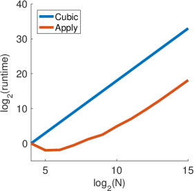
Figure 1. The scaling test of the evaluation of Equation (15) with an $N\times N$ matrix $M$, an $N\times N$ matrix $V$, and an $N^{2}\times 1$ vector $g_{kl}$. The runtime of the evaluation is recorded for different problem sizes $N$. Red: $\log_{2}(\text{runtime})$ as a function in $\log_{2}(N)$. Blue: ground truth cubic scaling line as a reference. The scaling is cubic when $N$ is sufficiently large.

3.2. Tests for the preconditioner

In the second part, we use synthetic Hamiltonian to construct approximate pp-RPA matrices. The Hamiltonian matrix $H$ is a discrete representation of the Hamiltonian operator

(19) $$\left(-\frac{\Delta}{2}+V(\mathbf{r})\right)\phi_{j}(\mathbf{r})=\epsilon_{j}\phi_{j}(\mathbf{r}),\qquad\mathbf{r}\in\ell\mathbb{T}^{d}:=[0,\ell)^{d},$$

with a periodic boundary condition and $d=1$ or $2$, where $V(\mathbf{r})$ is the potential field, $\epsilon_{j}$ is the orbital energy of the corresponding Kohn-Sham orbital, $\phi_{j}(\mathbf{r})$. It is convenient to rescale the system to the unit square via the transformation $\ell\mathbf{x}=\mathbf{r}$:

(20) $$\left(-\frac{\Delta}{2}+\ell^{d}V(\ell\mathbf{x})\right)\phi_{j}(\mathbf{x})=\epsilon_{j}\ell^{d}\phi_{j}(\mathbf{x}),\qquad\mathbf{x}\in\mathbb{T}^{d}:=[0,1)^{d},$$

and discretize the new system with the pseudo-spectral method. Let $V_{0}(\mathbf{r})$ be a Gaussian well on the unit domain $[0,1)^{d}$ (see Figure 2 (left) for an example when $d=2$) and extend it periodically with period $1$ to obtain $V(x)$ defined on $\ell\mathbb{T}^{d}:=[0,\ell)^{d}$. We randomly remove one Gaussian well from $V(x)$ to construct a non-trivial potential field and rescale it to $\ell^{d}V(\ell\mathbf{x})$ on the unit domain $[0,1)^{d}$ (see Figure 2 (right) for a two-dimensional example). The number of grid points per dimension within one period is set to $4$. Once the Hamiltonian is available, we compute its eigenpairs by direct diagonalization to obtain its orbitals $\{\phi_{p}\}_{1\leq p\leq N_{\text{grid}}}$ and the corresponding orbital energy $\{\epsilon_{p}\}_{1\leq p\leq N_{\text{grid}}}$.

We will use one-dimensional Hamiltonian matrices (i.e. $d=1$) to verify the efficiency of the proposed preconditioner in (17). The Jacobi-Davidson eigensolver in Algorithm 3 in the appendix is applied to compute the generalized eigenvalue closest to zero in the generalized eigenvalue problem (3), without any preconditioner and with the preconditioner in (17). Parameters in Algorithm 3 are $\epsilon=1e-10$, $m_{\min}=k_{\max}+5$, $m_{\max}=m_{\min}+5$, and $\text{mx}=400k_{\max}$. The initial nontrivial vector $\nu_{0}$ is one realization of a random vector such that each entry is a random variable with a uniform distribution in $[0,2]$.

Table 1 and 2 summarize the number of iterations and the accuracy of the eigensolver, respectively. As in the generalized eigenvalue problem (3), suppose the generalized eigenpair computed is $\left(\omega,\bigl{(}\begin{smallmatrix}X\\ Y\end{smallmatrix}\bigr{)}\right)$, the accuracy in Table 2 is defined to be the $2$-norm

$$\left\lVert\begin{pmatrix}A&B\\ B^{\top}&C\end{pmatrix}\begin{pmatrix}X\\ Y\end{pmatrix}-\omega\begin{pmatrix}I_{p}\\ &-I_{h}\end{pmatrix}\begin{pmatrix}X\\ Y\end{pmatrix}\right\rVert.$$

These results show that the proposed preconditioner is able to keep the number of iterations in the eigensolver roughly independent of the problem size, and the accuracy is usually higher in the presence of the preconditioner.

$\ell$	4	8	16	32	64	128
preconditioned	46	60	56	60	54	57
non-preconditioned	160	246	316	414	581	826

Table 1. The number of iterations in the Jacobi-Davidson eigensolver with and without a preconditioner. This table summarizes results for one-dimensional Hamiltonian matrices with different number of Gaussian wells $\ell$. The preconditioned eigensolver needs a number of iterations roughly independent of the problem size.

$\ell$	4	8	16	32	64	128
preconditioned	1.0e-09	1.1e-09	1.0e-09	1.2e-09	1.6e-08	5.6e-08
non-preconditioned	4.5e-10	7.1e-09	1.0e-08	6.0e-08	2.2e-02	2.4e-07

Table 2. The accuracy of the Jacobi-Davidson eigensolver with and without a preconditioner. This table summarizes results for one-dimensional Hamiltonian matrices with different number of Gaussian wells $\ell$.

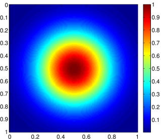
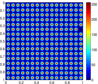
Figure 2. Left: the periodic function $V_{0}(\mathbf{r})$ is a Gaussian well on the unit square $[0,1)^{2}$. Right: the potential energy operator $\ell^{2}V(\mathbf{r})$ with $\ell=16$.

3.3. Tests for the truncated pp-RPA model

In this section, we construct Hamiltonian matrices, orbitals, and orbital energies using the same method in Section 3.2. We will conduct two sets of test to verify the truncation of orbital spaces in the pp-RPA model. In these tests, the Jacobi-Davidson eigensolver in Algorithm 3 in the appendix is applied to compute $k_{\max}$ (sufficiently many) generalized eigenvalues close to zero of pp-RPA matrices such that we able to obtain three positive eigenvalues closest to zero and three negative eigenvalues closest to zero. Other parameters in Algorithm 3 are $\epsilon=1e-10$, $m_{\min}=k_{\max}+5$, $m_{\max}=m_{\min}+5$, and $\text{mx}=400k_{\max}$. The initial nontrivial vector $\nu_{0}$ is one realization of a random vector such that each entry is a random variable with a uniform distribution in $[0,2]$.

In the first test, we verify the proposed truncated pp-RPA model by directly constructing the whole pp-RPA matrix in (18) (i.e., computing the repulsion integrals by naive summations) with different values of $N_{\text{vir}}$ and $N_{\text{occ}}$. When $N_{\text{vir}}$ and $N_{\text{occ}}$ are the total numbers of virtual and occupied orbitals, we obtain the original pp-RPA matrix in [Aggelen2013, Peng2013, Scuseria2013]. Let pct denote the percentage of occupied and virtual orbitals (with orbital energy closest to $\epsilon_{F}$) we used in the truncated pp-RPA model. We generate truncated pp-RPA matrices with $\text{pct}=0.05$, $0.1$, $0.2$, $0.3$, and $0.4$, compute three smallest positive eigenvalues and three largest negative eigenvalues by the Jacobi-Davidson method (denoted by $\text{val}_{\text{app}}\in\mathbb{R}^{6}$), compare these eigenvalues with those from the original pp-RPA matrix (denoted by $\text{val}_{\text{org}}\in\mathbb{R}^{6}$) via the relative difference below

(21) $$\text{err}=\max\bigl{\{}|\text{val}_{\text{app}}(k)-\text{val}_{\text{org}}(k)|/|\text{val}_{\text{org}}(k)|\bigr{\}}_{1\leq k\leq 6}.$$

Note that when $N_{\text{grid}}$ is small, $\text{pct}\cdot N_{\text{grid}}$ might be too small to establish a meaningful pp-RPA equation. Therefore, if $N_{\text{vir}}$ and $N_{\text{occ}}$ are smaller than $4$ due to a small pct, we will update $N_{\text{vir}}$ and $N_{\text{occ}}$ to $4$.

Table 3 and Table 4 summarize the relative difference err in these comparisons for one-dimensional and two-dimensional Hamiltonian matrices, respectively. These results show that, to estimate three smallest positive eigenvalues and three largest negative eigenvalues of the original pp-RPA matrix (i.e., the pp-RPA matrix constructed with all $N_{\text{grid}}$ orbitals using the naive implementation) within $4$-digits accuracy, it is sufficient to use only $10$ percents of both the occupied and the virtual orbitals to construct a truncated pp-RPA matrix via the naive implementation.

$\ell\backslash$ pct	0.05	0.1	0.2	0.3	0.4
4	9.9e-07	9.9e-07	9.9e-07	9.9e-07	1.8e-07
8	1.9e-07	1.9e-07	1.6e-07	1.4e-07	1.4e-07
16	2.8e-08	2.3e-08	2.2e-08	1.6e-08	1.0e-08
32	2.9e-09	2.5e-09	1.2e-09	3.8e-10	1.9e-10

Table 3. The relative difference err defined in (21) of three smallest positive eigenvalues and three largest negative eigenvalues of the original pp-RPA matrix and the truncated pp-RPA matrices constructed with different values of pct. Naive implementation is used in both cases. This table summarizes results for one-dimensional Hamiltonian matrices with different number of Gaussian wells $\ell=4$, $8$, $16$, and $32$.

$\ell\backslash$ pct	0.05	0.1	0.2	0.3	0.4
2	3.2e-04	1.8e-04	5.7e-05	2.3e-05	1.5e-05
3	5.0e-06	3.4e-06	3.2e-06	3.1e-06	3.1e-06

Table 4. The relative difference err defined in (21) of three smallest positive eigenvalues and three largest negative eigenvalues of the original pp-RPA matrix and the truncated pp-RPA matrices constructed with different values of pct. Naive implementation is used in both cases. This table summarizes results for two-dimensional Hamiltonian matrices with different number of Gaussian wells $\ell^{2}=4$ and $9$.

In the second test, we verify the truncated pp-RPA model by applying the proposed fast matvec to compute the eigenvalues of the truncated pp-RPA matrices with different values of $N_{\text{vir}}$ and $N_{\text{occ}}$. When $N_{\text{vir}}$ and $N_{\text{occ}}$ are the total numbers of virtual and occupied orbitals, we approximately obtain the original pp-RPA matrix in [Aggelen2013, Peng2013, Scuseria2013] up to some error introduced by the density fitting. In the construction of the interpolative separable density fitting, we set the parameter $\epsilon=1e-7$ and $c=10$. Again, we generate truncated pp-RPA matrices with $\text{pct}=0.05$, $0.1$, $0.2$, $0.3$, and $0.4$, compute three smallest positive eigenvalues and three largest negative eigenvalues by the Jacobi-Davidson method (denoted by $\text{val}_{\text{app}}\in\mathbb{R}^{6}$), compare these eigenvalues with those from the original pp-RPA matrix (denoted by $\text{val}_{\text{org}}\in\mathbb{R}^{6}$) by computing the relative difference as in (21). Since in the first test, we have computed the ground truth eigenvalues from the exact pp-RPA matrix by direct evaluation, we reuse these eigenvalues if available, instead of using the eigenvalues of the truncated pp-RPA matrix when $\text{pct}=1$.

Table 5 and Table 6 summarize these comparisons for one-dimensional and two-dimensional Hamiltonian matrices, respectively. These results lead to the same conclusion as in the first test.

$\ell\backslash$ pct	0.05	0.1	0.2	0.3	0.4
4	9.9e-07	9.9e-07	9.9e-07	9.9e-07	1.8e-07
8	1.9e-07	1.9e-07	1.6e-07	1.4e-07	1.4e-07
16	2.8e-08	2.3e-08	2.2e-08	1.6e-08	1.0e-08
32	2.9e-09	2.5e-09	1.2e-09	3.8e-10	1.9e-10
64	3.0e-10	1.4e-10	4.3e-11	2.1e-11	9.6e-12
128	1.6e-11	6.5e-12	2.4e-12	5.0e-08	5.7e-13
256	8.3e-13	4.0e-13	1.5e-13	7.0e-14	3.5e-14

Table 5. The relative difference err defined in (21) of three smallest positive eigenvalues and three largest negative eigenvalues of the original pp-RPA matrix and the truncated pp-RPA matrices constructed with different values of pct. This table summarizes results for one-dimensional Hamiltonian matrices with different number of Gaussian wells $\ell=4$, $8$, $\dots$, and $256$. The cubic scaling algorithm is used for truncated pp-RPA, for the original pp-RPA, naive implementation is used when $\ell=4$, $\dots$, and $32$, and cubic scaling algorithm is used when $\ell=64$, $128$, and $256$ since the naive algorithm is too slow.

$\ell\backslash$ pct	0.05	0.1	0.2	0.3	0.4
2	3.2e-04	1.8e-04	5.7e-05	2.3e-05	1.5e-05
3	5.0e-06	3.4e-06	3.2e-06	2.8e-05	3.1e-06
4	2.8e-05	2.1e-05	1.8e-05	1.7e-05	1.3e-05
5	9.1e-05	9.1e-05	9.1e-05	1.2e-06	7.7e-07

Table 6. The relative difference err defined in (21) of three smallest positive eigenvalues and three largest negative eigenvalues of the original pp-RPA matrix and the truncated pp-RPA matrices constructed with different values of pct. This table summarizes results for two-dimensional Hamiltonian matrices with different number of Gaussian wells $\ell^{2}=4$, $9$, $16$, and $25$. The cubic scaling algorithm is used for truncated pp-RPA, for the original pp-RPA, naive implementation is used when $\ell^{2}=4$ and $9$, and cubic scaling algorithm is used when $\ell^{2}=16$ and $25$ since the naive algorithm is too slow.

Appendix A The Jacobi-Davidson eigensolver

In Algorithm 3 we describe the Jacobi-Davidson algorithm [JDgeig, Gerard2000] to compute $k_{\max}$ generalized eigenpairs with generalized eigenvalues closest to a target $\tau$. In particular, if low-lying excitations are desired, we can take $\tau=0$ in the algorithm. The algorithm description follows the lecture note by Peter Arbenz available at http://people.inf.ethz.ch/arbenz/ewp/Lnotes/chapter12.pdf, and the codes are available at Gerard L.G. Sleijpen’s personal homepage: http://www.staff.science.uu.nl/~sleij101/.

1

Input : Square matrices $A$ and $B$ in $\mathbb{C}^{n\times n}$, $\tau$, $k_{\max}$, the accuracy parameter $\epsilon$, restart parameters $m_{\min}$ and $m_{\max}$, the maximum number of iterations mx.

Output : $Q$ and $Z\in\mathbb{C}^{n\times k_{\max}}$, $R^{A}$ and $R^{B}\in\mathbb{C}^{k_{\max}\times k_{\max}}$ s.t.$AQ=ZR^{A}$ and $BQ=ZR^{B}$. The $k_{\max}$ interior generalized eigenvalues close to the target $\tau$ are $\{R^{A}_{k,k}/R^{B}_{k,k}\}_{1\leq k\leq k_{\max}}$.

2

3Choose a nontrivial vector $v_{0}$; $k=0$; $\nu_{0}=1/\sqrt{1+|\tau|^{2}}$; $\mu_{0}=-\tau\nu_{0}$; $m=0$; $\text{itr}=0$;

4$Q=[]$; $Z=[]$; $S=[]$; $T=[]$;

5while $k<k_{\max}$ and $\text{itr}<\text{mx}$ do

6       Orthogonalize $t\leftarrow t-V_{m}V_{m}^{*}t$;

7      $\text{itr}\leftarrow\text{itr}+1$; $m=m+1$; $v_{m}=t/\|t\|$; $v^{A}_{m}=Av_{m}$; $v^{B}_{m}=Bv_{m}$; $w=\nu_{0}v^{A}_{m}+\mu_{0}v^{B}_{m}$;

8      Orthogonalize: $w\leftarrow w-Z_{k}Z_{k}^{*}w$; $w\leftarrow w-W_{m-1}W_{m-1}^{*}w$; $w_{m}=w/\|w\|$;

9      $\displaystyle M^{A}\leftarrow\begin{pmatrix}M^{A}&W_{m-1}^{*}v^{A}_{m}\\ w_{m}^{*}V^{A}_{m-1}&w_{m}^{*}v^{A}_{m}\end{pmatrix};\quad M^{B}\leftarrow\begin{pmatrix}M^{B}&W_{m-1}^{*}v^{B}_{m}\\ w_{m}^{*}V^{B}_{m-1}&w_{m}^{*}v_{m}^{B}\end{pmatrix};$

10      Compute the $QZ$ decomposition $M^{A}S^{R}=S^{L}T^{A}$, $M^{B}S^{R}=S^{L}T^{B}$, such that $|T^{A}_{i,i}/T^{B}_{i,i}-\tau|\leq|T^{A}_{i+1,i+1}/T^{B}_{i+1,i+1}-\tau|$ (the Rayleigh-Ritz step);

11      $u=Vs^{R}_{1}$; $p=W_{j}s^{L}_{1}$; $u^{A}=V^{A}s^{R}_{1}$; $u^{B}=V^{B}s^{R}_{1}$; $\zeta=T^{A}_{1,1}$; $\eta=T^{B}_{1,1}$;

12      $r=\eta u^{A}-\zeta u^{B}$; $\widetilde{a}=Z^{*}u^{B}$; $\widetilde{b}=Z^{*}u^{B}$; $\widetilde{r}=r-Z(\eta\widetilde{a}-\zeta\widetilde{b})$;

13      while $\|\widetilde{r}\|<\epsilon$ do

14             $\displaystyle R^{A}\leftarrow\begin{pmatrix}R^{A}&\widetilde{a}\\ 0^{\top}&\zeta\end{pmatrix};\quad R^{B}\leftarrow\begin{pmatrix}R^{B}&\widetilde{b}\\ 0^{\top}&\eta\end{pmatrix};$

15            $Q\leftarrow[Q,u]$; $Z\leftarrow[Z,p]$; $k\leftarrow k+1$; $m\leftarrow m-1$;

16            if $k=k_{\max}$ then

17                   return $(Q,Z,R^{A},R^{B})$

18            

19            for $i=1,\dots,m$ do

20                   $v_{i}=Vs^{R}_{i+1}$; $v^{A}_{i}=V^{A}s^{R}_{i+1}$; $v^{B}_{i}=V^{B}s^{R}_{i+1}$;

21                  $w_{i}=Ws^{L}_{i+1}$; $s^{R}_{i}=s^{L}_{i}=e_{i}$;

22            

23            $M^{A}$, $M^{B}$ is the lower $m\times m$ block of $T^{A}$, $T^{B}$, respectively.

24            $u=u_{1}$; $p=w_{1}$; $u^{A}=v^{A}_{1}$; $u^{B}=v^{B}_{1}$; $\zeta=T^{A}_{1,1}$; $\eta=T^{B}_{1,1}$;

25            $r=\eta u^{A}-\zeta u^{B}$; $\widetilde{a}=Z^{*}u^{A}$; $\widetilde{b}=Z^{*}u^{B}$; $\widetilde{r}=r-Z(\eta\widetilde{a}-\zeta\widetilde{b})$;

26      

27      if $m\geq m_{max}$ then

28             for $i=2,\dots,m_{\min}$ do

29                   $v_{i}=Vs^{R}_{i}$; $v^{A}_{i}=V^{A}s^{R}_{i}$; $v^{B}_{i}=V^{B}s^{R}_{i}$; $w_{i}=Ws^{L}_{i}$;

30            

31            $M^{A}$, $M^{B}$ is the leading $m_{\min}\times m_{\min}$ block of $T^{A}$, $T^{B}$, respectively.

32            $v_{1}=u$; $v^{A}_{1}=u^{A}$;$v^{B}_{1}=u^{B}$; $w_{1}=p$; $m=m_{\min}$.

33      

34      $\widetilde{Q}=[Q,u]$; $\widetilde{Z}=[X,p]$;

35      (Approximately) solve the correction equation for $t\perp\widetilde{Q}$ using GMRES, $(I-\widetilde{Z}\widetilde{Z}^{*})(\eta A-\zeta B)(I-\widetilde{Q}\widetilde{Q}^{*})t=-r$, where $r=\eta Au^{A}-\zeta Bu^{B}$.

36

Algorithm 3 Jacobi-Davidson QZ method for $k_{\max}$ interior eigenvalues close to $\tau$.