Astronomy Letters, 2017, Vol. 43, Issue 3

THE GALAXY KINEMATICS FROM OB STARS

WITH PROPER MOTIONS FROM THE GAIA DR1 CATALOG

V.V. Bobylev, A.T. Bajkova

Central (Pulkovo) Astronomical Observatory, Russian Academy of Sciences

We consider two previously studied samples of OB stars with different distance scales. The first one consists of massive spectroscopic binary stars with photometric distances, and the second one  — with the distances determined along the lines of interstellar calcium. The OB-stars are located at distances up to 7 kpc from the Sun. They are identified with the Gaia DR1 catalog. It is shown that the use of the proper motions, taken from the Gaia DR1 catalog, allows to reduce random errors of determination of the Galactic rotation parameters in comparison with the previously known ones. From the analysis of 208 OB stars from the Gaia DR1 catalog with proper motions and parallaxes with relative errors less than 200% were found the following values of kinematic parameters: $(U,V)_{\odot}=(8.67,6.63)\pm(0.88,0.98)$ km s^-1, $\Omega_{0}=27.35\pm 0.77$ km s^-1 kpc^-1, $\Omega^{{}^{\prime}}_{0}=-4.13\pm 0.13$ km s^-1 kpc^-2, $\Omega^{{}^{\prime\prime}}_{0}=0.672\pm 0.070$ km s^-1 kpc^-3, the Oort constants $A=-16.53\pm 0.52$ km s^-1 kpc^-1 and $B=10.82\pm 0.93$ km s^-1 kpc^-1, linear circular velocity of the Local Standard of Rest around the Galactic center $V_{0}=219\pm 8$ km s^-1 for an adopted value of $R_{0}=8.0\pm 0.2$ kpc. In addition the Galactic rotation parameters were obtained from only line-of-sight velocities of the same stars. From the comparison of these two values of $\Omega^{{}^{\prime}}_{0}$ a distance scale of the Gaia DR1 catalog was determined as a value close to unit, namely 0.96. From 238 OB-stars of the united sample with photometric distances for stars of the first sample and distances in the calcium scale for stars of the second sample, line-of-sight velocities and proper motions from the Gaia DR1 catalog, were found the following values of the kinematic parameters: $(U,V,W)_{\odot}=(8.19,9.28,8.79)\pm(0.74,0.92,0.74)$ km s^-1, $\Omega_{0}=31.53\pm 0.54$ km s^-1 kpc^-1, $\Omega^{{}^{\prime}}_{0}=-4.44\pm 0.12$ km s^-1 kpc^-2, $\Omega^{{}^{\prime\prime}}_{0}=0.706\pm 0.100$ km s ^-1 kpc^-3, here Oort constants: $A=-17.77\pm 0.46$ km s^-1 kpc^-1, $B=13.76\pm 0.71$ km s^-1 kpc^-1 and $V_{0}=252\pm 8$ km s^-1.

INTRODUCTION

From the combination of the first year Gaia observational data(Prusti et al., 2016) with the positions and proper motions of Tycho-2 (Høg et al., 2000) stars was created the Gaia DR1 catalog. It is referred to as TGAS (Tycho–Gaia Astrometric Solution, Mihalik, et al., 2015; Brown et al., 2016; Lindegren et al., 2016), and contains parallaxes and proper motion of about 2 million brightest stars (up to $\sim 11.^{m}5$).

Random errors of data included in the Gaia DR1 catalog are comparable or less than those given in the HIPPARCOS (1997) and Tycho-2 catalogs. Average errors of parallaxes are about 0.3 mas (milliarcseconds). It means that with distances with errors of about 10% it is possible to cover the Solar neighborhood with a radius only of about 300 pc. Therefore, when studying the structure and kinematics of the Galaxy at larger distances from the Sun (3 kpc, and more) currently remains relevant approach using photometric or other distance scales.

For most of the TGAS stars an average error of proper motion is about 1 mas/yr (milliarcseconds per year). But for a significant number ($\sim$94000) of the HIPPARCOS catalog stars this error is an order of magnitude smaller and is about 0.06 mas/yr (Brown et al., 2016). Therefore, the analysis of their spatial velocities using high-precision proper motions is of great interest.

In this work two samples of OB stars are used. The first sample consists of young massive OB stars with photometric estimates of distances, most of them are spectroscopic binary stars. This sample was compiled by Bobylev&Bajkova (2013; 2015) on published sources, and it contains about 300 OB stars. The second sample basically consists of single OB stars, with distances defined by the spectral lines of interstellar calcium. These distances are determined by Megier et al. (2005; 2009) and Galazutdinov et al. (2015). The study of this sample with star proper motions from the HIPPARCOS catalog was made by Bobylev&Bajkova (2011; 2015).

The aim of this work is testing of the distance scale of the Gaia DR1 catalog, re-determining the Galactic rotation parameters from data on OB stars with proper motions from the Gaia DR1 catalog. We analyze full spatial velocities of OB stars as well as the velocities determined only from proper motions or only from line-of-sight velocities.

METHODS

From observations we know three components of the star velocity: the line-of-sight velocity $V_{r}$ and the two projections of the tangential velocity $V_{l}=4.74r\mu_{l}\cos b$ and $V_{b}=4.74r\mu_{b},$ directed along the Galactic longitude $l$ and latitude $b$ respectively and expressed in km s^-1. Here the coefficient 4.74 is the ratio of the number of kilometers in astronomical unit by the number of seconds in a tropical year, and $r$ is a heliocentric distance of the star in kpc. The components of a proper motion of $\mu_{l}\cos b$ and $\mu_{b}$ are expressed in the mas yr^-1. The velocities $U,V,W$ directed along the rectangular Galactic coordinate axes are calculated via the components of $V_{r},V_{l},V_{b}$:

$$\begin{array}[]{lll}U=V_{r}\cos l\cos b-V_{l}\sin l-V_{b}\cos l\sin b,\\ V=V_{r}\sin l\cos b+V_{l}\cos l-V_{b}\sin l\sin b,\\ W=V_{r}\sin b+V_{b}\cos b,\end{array}$$ (1)

where $U$ is directed from the Sun to the Galactic center, $V$ is in the direction of Galactic rotation, and $W$ is directed toward the north Galactic pole. We can find two velocities, $V_{R}$ directed radially away from the Galactic center and $V_{circ}$ orthogonal to it and pointing in the direction of Galactic rotation, based on the following relations:

$$\begin{array}[]{lll}V_{circ}=U\sin\theta+(V_{0}+V)\cos\theta,\\ V_{R}=-U\cos\theta+(V_{0}+V)\sin\theta,\end{array}$$ (2)

where the position angle $\theta$ satisfies to the ratio $\tan\theta=y/(R_{0}-x)$, and $x,y,z$ are rectangular heliocentric coordinates of the star (velocities $U,V,W$ are directed along the axes $x,y,z$ respectively).

To determine the parameters of the Galactic rotation curve, we use the equation derived from Bottlinger’s formulas in which the angular velocity $\Omega$ was expanded in a series to terms of the second order of smallness in $r/R_{0}$:

$$\begin{array}[]{lll}V_{r}=-U_{\odot}\cos b\cos l-V_{\odot}\cos b\sin l\\ -W_{\odot}\sin b+R_{0}(R-R_{0})\sin l\cos b\Omega^{{}^{\prime}}_{0}+0.5R_{0}(R-R_{0})^{2}\sin l\cos b\Omega^{{}^{\prime\prime}}_{0},\end{array}$$ (3)

$$\begin{array}[]{lll}V_{l}=U_{\odot}\sin l-V_{\odot}\cos l-r\Omega_{0}\cos b\\ +(R-R_{0})(R_{0}\cos l-r\cos b)\Omega^{{}^{\prime}}_{0}+0.5(R-R_{0})^{2}(R_{0}\cos l-r\cos b)\Omega^{{}^{\prime\prime}}_{0},\end{array}$$ (4)

$$\begin{array}[]{lll}V_{b}=U_{\odot}\cos l\sin b+V_{\odot}\sin l\sin b\\ -W_{\odot}\cos b-R_{0}(R-R_{0})\sin l\sin b\Omega^{{}^{\prime}}_{0}-0.5R_{0}(R-R_{0})^{2}\sin l\sin b\Omega^{{}^{\prime\prime}}_{0},\end{array}$$ (5)

where $R$ is the distance from the star to the Galactic rotation axis,

$$R^{2}=r^{2}\cos^{2}b-2R_{0}r\cos b\cos l+R^{2}_{0}.$$ (6)

$\Omega_{0}$ is the angular velocity of Galactic rotation at the solar distance $R_{0}$, the parameters $\Omega^{{}^{\prime}}_{0}$ and $\Omega^{{}^{\prime\prime}}$ are the corresponding derivatives of the angular velocity, and $V_{0}=|R_{0}\Omega_{0}|$.

It is necessary to adopt a certain value of the distance $R_{0}$. One of the most reliable estimates of this value $R_{0}=8.28\pm 0.29$ kpc obtained by Gillessen et al. (2009) from the analysis of the orbits of the stars, moving around the supermassive black hole at the center of the Galaxy. From masers with trigonometric parallaxes Reid et al. (2014) found $R_{0}=8.34\pm 0.16$ kpc. From analysis of kinematics of the masers Bobylev&Bajkova (2014) estimated $R_{0}=8.3\pm 0.2$ kpc, in work by Bajkova&Bobylev (2015) it is found $R_{0}=8.03\pm 0.12$ kpc, Rastorguev et al.(2016) obtained $R_{0}=8.40\pm 0.12$ kpc. Recent analysis of the orbits of stars moving around the supermassive black hole at the center of the Galaxy gave an estimate $R_{0}=7.86\pm 0.2$ kpc (Boehle et al., 2016). In the present work the adopted value $R_{0}=8.0\pm 0.2$ kpc.

The influence of the spiral density wave in the radial, $V_{R},$ and residual tangential, $\Delta V_{circ},$ velocities is periodic with an amplitude of $\sim$10 km s${}^{-1}.$ According to the linear theory of density waves (Lin and Shu 1964), it is described by the following relations:

$$\begin{array}[]{lll}V_{R}=-f_{R}\cos\chi,\\ \Delta V_{circ}=f_{\theta}\sin\chi,\end{array}$$ (7)

where

$$\chi=m[\cot(i)\ln(R/R_{0})-\theta]+\chi_{\odot}$$ (8)

is the phase of the spiral density wave ($m$ is the number of spiral arms, $i$ is the pitch angle of the spiral pattern, $\chi_{\odot}$ is the radial phase of the Sun in the spiral density wave); $f_{R}$ and $f_{\theta}$ are the radial and tangential velocity perturbation amplitudes, which are assumed to be positive.

We apply a spectral analysis to study the periodicities in the velocities $V_{R}$ and $\Delta V_{circ}$. The wavelength $\lambda$ (the distance between adjacent spiral arm segments measured along the radial direction) is calculated from the relation

$$\frac{2\pi R_{0}}{\lambda}=m\cot(i).$$ (9)

Let there be a series of measured velocities $V_{R_{n}}$ (these can be both radial, $V_{R}$ and residual tangential, $\Delta V_{\theta},$ velocities), $n=1,\dots,N$, where $N$ is the number of objects. The objective of our spectral analysis is to extract a periodicity from the data series in accordance with the adopted model describing a spiral density wave with parameters $f_{R},\lambda(i)$ and $\chi_{\odot}$.

Having taken into account the logarithmic character of the spiral density wave and the position angles of the objects $\theta_{n},$ our spectral (periodogram) analysis of the series of velocity perturbations is reduced to calculating the square of the amplitude (power spectrum) of the standard Fourier transform (Bajkova&Bobylev 2012):

$$\bar{V}_{\lambda_{k}}=\frac{1}{N}\sum_{n=1}^{N}V^{{}^{\prime}}_{n}(R^{{}^{\prime}}_{n})\exp\Bigl{(}-j\frac{2\pi R^{{}^{\prime}}_{n}}{\lambda_{k}}\Bigr{)},$$ (10)

where $\bar{V}_{\lambda_{k}}$ is the $k$th harmonic of the Fourier transform with wavelength $\lambda_{k}=D/k,D$ is the period of the series being analyzed,

$$\begin{array}[]{lll}R^{{}^{\prime}}_{n}=R_{\circ}\ln(R_{n}/R_{\circ}),\\ V^{{}^{\prime}}_{n}(R^{{}^{\prime}}_{n})=V_{n}(R^{{}^{\prime}}_{n})\times\exp(jm\theta_{n}).\end{array}$$ (11)

The algorithm of searching for periodicities modified to properly determine not only the wavelength but also the amplitude of the perturbations is described in detail in Bajkova and Bobylev (2012).

The peak value of the power spectrum $S_{peak}$ corresponds to the sought-for wavelength $\lambda$. The pitch angle of the spiral density wave is found from the expression (9). Amplitude and phase of perturbations we obtain by the fit of the harmonic with found wavelength to the measured data. To evaluate the amplitude of perturbations the following relation can also be used:

$$f_{R}(f_{\theta})=\sqrt{4\times S_{peak}}.$$ (12)

So, our approach consists of two stages: a)constructing a smooth Galactic rotation curve, and b)spectral analysis of radial $V_{R},$ and residual tangential $\Delta V_{circ}$ velocities. Similar approach has been applied by Bobylev et al. (2008) for studying the kinematics of young Galactic objects, by Bobylev&Bajkova (2012) for analysis of the Cepheids, and by Bobylev&Bajkova (2013; 2015) to determine the Galactic rotation curve from data on massive OB-stars.

DATA

In the present work we use the following two samples of OB stars: 1) the sample of spectroscopic binary OB stars and 2) the sample of OB stars with distances determined by the spectral lines of the interstellar Ca II.

The catalog of massive spectroscopic binary stars is described by Bobylev&Bajkova (2013; 2015). There we considered the systems with the spectra of the main component no later than B2.5 and different super giants with luminosity classes Ia and Iab. In addition, from the HIPPARCOS catalog we took all the B2.5-stars with relative errors of parallaxes less than 10%. For all stars in this catalog, there are estimates of distances, line-of sight velocities and proper motions. In the end, were collected data on 120 spectroscopic binary and single stars that do not have properties of “runaway” stars, because their residual velocities do not exceed 40–50 km s^-1. We identified 98 stars from this catalog with the stars of Gaia DR1 catalog.

The spectroscopic method of determining star distances using broadening of the absorption lines of the interstellar ionized atoms Ca II, Na I, or K I is well known. Megier et al. (2005; 2009) bound the scale of the equivalent widths to trigonometric parallaxes of the HIPPARCOS catalogue. It turned out that the Ca II spectral line widths are measured with the most high accuracy, therefore we call this scale as a calcium scale. According to the estimates of Megier et al. (2009), the average accuracy of individual distance to OB stars is approximately 15%.

From the analysis of several kinematic parameters obtained from data on distant OB stars of this sample, Bobylev&Bajkova (2011) showed the need for small, no more than 20%, reducing of the scale of distances to stars which are further 0.8 kpc from the Sun. Accounting for the measurements of Galazutdinov et al. (2015), the whole sample contains 340 OB stars, 168 stars of which were identified with the stars of the Gaia DR1 catalog.

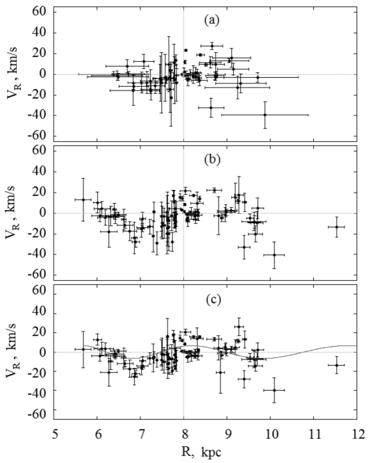
Figure 1: Radial velocities $V_{R}$ versus $R$ of spectroscopic binary OB stars: a) with distances with relative errors less than 60% and proper motions from the Gaia DR1 catalog, b)  with photometric distances and proper motions from the HIPPARCOS catalog, c) with photometric distances and proper motions from the Gaia DR1 catalog.

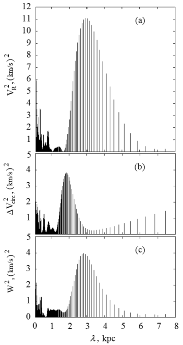
Figure 2: Power spectra for the spectroscopic binary OB stars with photometric distances and proper motions from the Gaia DR1 catalog: a) of the radial velocities $V_{R}$, b) of the residual circular rotation velocities $\Delta V_{circ}$ b) and c) of the vertical $W$ velocities.

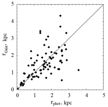
Figure 3: The distances to the stars from the Gaia DR1 catalog versus distances to the same stars, determined by the photometric method; a straight line corresponds to the correlation equal to 1.

RESULTS AND DISCUSSION

The system of conditional equations (3)–(5) was solved by the least squares method with the following weights $w_{r}=S_{0}/\sqrt{S_{0}^{2}+\sigma^{2}_{V_{r}}},$ $w_{l}=S_{0}/\sqrt{S_{0}^{2}+\sigma^{2}_{V_{l}}}$ and $w_{b}=S_{0}/\sqrt{S_{0}^{2}+\sigma^{2}_{V_{b}}},$ where $S_{0}$ is a “cosmic” dispersion, $\sigma_{V_{r}},\sigma_{V_{l}},\sigma_{V_{b}}$  are appropriate error variances of the observational velocities. The value of $S_{0}$ is comparable to the mean square residual $\sigma_{0}$ (error of unit weight) in the solution of conditional equations (3)–(5). In the present work $S_{0}=8$ km s^-1 is adopted. For the exclusion of runaway stars, we use the following restriction:

$$\begin{array}[]{lll}\sqrt{U^{2}+V^{2}+W^{2}}<80~{}\hbox{km s${}^{-1}$},\end{array}$$ (13)

where the velocities $U,V,W$ are residual, they are exempt from differential rotation of the Galaxy using found pre-rotation parameters (or already known). Solutions are searched in two iterations with the exception of large residuals according to the criterion $3\sigma$.

Sample of spectroscopic binary stars

In the first step for 98 spectroscopic binary stars subject to the criterion of (13) the original photometric distances and proper motions were taken from the HIPPARCOS and Tycho-2 catalogs. From these data were found the following kinematic parameters:

$$\begin{array}[]{lll}(U_{\odot},V_{\odot},W_{\odot})=(2.7,9.2,10.4)\pm(1.0,1.2,1.1)~{}\hbox{km s${}^{-1}$},\\ \Omega_{0}=~{}28.95\pm 0.84~{}\hbox{km s${}^{-1}$ kpc${}^{-1}$},\\ \Omega^{{}^{\prime}}_{0}=-4.15\pm 0.17~{}\hbox{km s${}^{-1}$ kpc${}^{-2}$},\\ \Omega^{{}^{\prime\prime}}_{0}=~{}1.019\pm 0.155~{}\hbox{km s${}^{-1}$ kpc${}^{-3}$}.\end{array}$$ (14)

In this solution, the error of unit weight is $\sigma_{0}=9.7$ km s^-1, the Oort constants: $A=-16.61\pm 0.69$ km s^-1 kpc^-1 and $B=12.35\pm 1.08$ km s^-1 kpc^-1. The number of equations was 268.

The solution (14) should be compared with the obtained by Bobylev&Bajkova (2015) from data on 120 OB stars of this sample: $(U_{\odot},V_{\odot},W_{\odot})=(2.8,9.2,9.3)\pm(1.0,1.2,1.0)$ km s^-1, $\Omega_{0}=29.3\pm 0.8$ km s^-1 kpc^-1, $\Omega^{{}^{\prime}}_{0}=-4.28\pm 0.15$ km s^-1 kpc^-2, $\Omega^{{}^{\prime\prime}}_{0}=0.957\pm 0.128$ km s^-1 kpc^-3, where the value of the error of unit weight is $\sigma_{0}=10.5$ km s^-1, the linear velocity of the Galactic rotation $V_{0}=234\pm 14$ km s^-1 (for $R_{0}=8.0\pm 0.4$ kpc), and the Oort constants: $A=-17.1\pm 0.6$ km s^-1 kpc^-1 and $B=12.2\pm 1.0$ km s^-1 kpc^-1.

In the second step for these 98 stars the original photometric distances and proper motions from the Gaia DR1 catalog were taken. From these data we found the following kinematic parameters:

$$\begin{array}[]{lll}(U_{\odot},V_{\odot},W_{\odot})=(3.8,8.5,8.4)\pm(0.9,1.1,0.9)~{}\hbox{km s${}^{-1}$},\\ \Omega_{0}=~{}30.91\pm 0.74~{}\hbox{km s${}^{-1}$ kpc${}^{-1}$},\\ \Omega^{{}^{\prime}}_{0}=-4.27\pm 0.15~{}\hbox{km s${}^{-1}$ kpc${}^{-2}$},\\ \Omega^{{}^{\prime\prime}}_{0}=~{}0.911\pm 0.130~{}\hbox{km s${}^{-1}$ kpc${}^{-3}$}.\end{array}$$ (15)

In this solution, the error of unit weight is $\sigma_{0}=8.3$ km s^-1, the Oort constants: $A=-17.08\pm 0.59$ km s^-1 kpc^-1 and $B=13.83\pm 0.95$ km s^-1 kpc^-1. The number of equations was 265.

In Fig. 1 the radial velocities $V_{R}$ versus $R$ are shown for three cases. The first case represents 60 spectroscopic binary stars with distances with relative errors less than 60% and the proper motions taken from the Gaia DR1 catalog. In the second case the stars with the photometric distances and the proper motions from the HIPPARCOS, Tycho-2 and UCAC4 catalogs were used, as in the solution (14). In the third case the spectroscopic binary OB stars with the photometric distances and the proper motions from the Gaia DR1 catalog were used, as in the solution (15).

Based on the parameters of the rotation curve represented by the solution (15), we obtained the residual tangential velocities $\Delta V_{circ}$. In Fig. 2 the power spectra of the radial velocities $V_{R}$, the residual tangential velocities $\Delta V_{circ}$ and the vertical $W$ ones are shown. From figure you can see that the power spectrum of the radial velocities has the largest amplitude.

The parameters of the galactic spiral density wave were obtained using periodogram analysis of series of the residual tangential $\Delta V_{circ},$ radial $V_{R}$ and vertical $W$ velocities. The amplitudes of the tangential, radial and vertical velocity perturbations $f_{\theta}=3.9\pm 1.6$ km s^-1, $f_{R}=6.7\pm 1.2$ km s^-1, $f_{W}=4.0\pm 1.1$ km s^-1 respectively, wavelength of the perturbations $\lambda_{\theta}=1.9\pm 0.6$ kpc, $\lambda_{R}=2.9\pm 0.4$ kpc and $\lambda_{W}=2.8\pm 0.4$ kpc for adopted four-armed spiral pattern model ($m=4$). The Sun’s phase in the spiral density wave $(\chi_{\odot})_{\theta}=-132^{\circ}\pm 14^{\circ}$ from the residual tangential velocities, $(\chi_{\odot})_{R}=-157^{\circ}\pm 10^{\circ}$ from the radial velocities and $(\chi_{\odot})_{W}=-159^{\circ}\pm 11^{\circ}$ from the vertical velocities. The bottom panel of Fig. 1 shows the wave in the radial velocities, constructed from the parameters found above.

You can see that the parameters of the velocity perturbations found in the residual tangential velocities are determined with large relative errors, i.e. at these velocities is it difficult to see the direct influence of the spiral density wave, perhaps there is a more complicated picture than we have modelled. On the contrary, the parameters of the velocity perturbation, found in the radial and vertical velocities are a in good agreement with each other.

The values of the parameters of the spiral density wave found in the radial velocities $V_{R}$, are in good agreement with the estimated ones obtained for 120 stars of this sample by Bobylev&Bajkova (2015). However, in this work we see a good agreement between the parameters found in the radial and vertical velocities (except for amplitudes), while in the work of Bobylev&Bajkova (2015), it was mentioned a poor agreement between the estimates of these parameters.

Based on the 87 OB-stars with relative errors of distances from the Gaia DR1 catalog, not exceeding 200%, there was built Fig. 3. On it the distances to the stars from the Gaia DR1 catalog versus the distances to these stars determined by photometric method are given. We can see that there is practically no significant systematic differences between these two scales of distances. When the relative errors of distances from the Gaia DR1 catalog are more than 200%, the points in the figure strongly deviate upward from the straight line. Therefore, when such large errors the distances from the Gaia DR1 catalog are undesirable to use.

Sample of OB stars with the calcium distance scale

In the first step, for 160 stars of this sample that satisfy the criterion (13), the distances in the calcium scale and the proper motions from the HIPPARCOS and Tycho-2 catalogs were used. The distances of the stars were multiplied by a scaling factor 0.8, except those which are close to the Sun ($r<0.8$ kpc).

Using these stars we found the following kinematic parameters:

$$\begin{array}[]{lll}(U_{\odot},V_{\odot},W_{\odot})=(10.0,9.9,9.4)\pm(1.2,1.6,1.2)~{}\hbox{km s${}^{-1}$},\\ \Omega_{0}=~{}29.15\pm 0.93~{}\hbox{km s${}^{-1}$ kpc${}^{-1}$},\\ \Omega^{{}^{\prime}}_{0}=-4.35\pm 0.19~{}\hbox{km s${}^{-1}$ kpc${}^{-2}$},\\ \Omega^{{}^{\prime\prime}}_{0}=~{}0.874\pm 0.153~{}\hbox{km s${}^{-1}$ kpc${}^{-3}$}.\end{array}$$ (16)

In this solution, the error of unit weight is $\sigma_{0}=14.7$ km s^-1, the Oort constants: $A=-17.40\pm 0.74$ km s^-1 kpc^-1 and $B=11.75\pm 1.18$ km s^-1 kpc^-1. The number of equations was 448.

In the second step, for these 160 stars with the same distances, the proper motions were taken from the Gaia DR1 catalog. From these data the following kinematics parameters were found:

$$\begin{array}[]{lll}(U_{\odot},V_{\odot},W_{\odot})=(10.7,9.1,9.0)\pm(1.0,1.3,1.0)~{}\hbox{km s${}^{-1}$},\\ \Omega_{0}=~{}31.17\pm 0.70~{}\hbox{km s${}^{-1}$ kpc${}^{-1}$},\\ \Omega^{{}^{\prime}}_{0}=-4.54\pm 0.15~{}\hbox{km s${}^{-1}$ kpc${}^{-2}$},\\ \Omega^{{}^{\prime\prime}}_{0}=~{}0.788\pm 0.123~{}\hbox{km s${}^{-1}$ kpc${}^{-3}$}.\end{array}$$ (17)

In this solution, the error of unit weight is $\sigma_{0}=12.3$ km s^-1, the Oort constants: $A=-18.14\pm 0.59$ km s^-1 kpc^-1 and $B=13.03\pm 0.91$ km s^-1 kpc^-1. The number of equations was 465.

We can see that the use of proper motions, taken from the Gaia DR1 catalog for the analysis of the stars of both the first and the second samples, reduces random errors of estimation of the Galactic rotation parameters at comparison with the previously known results.

OB stars with data from the Gaia DR1 catalog

In the Gaia DR1 catalog there is no information allowing accurate spectral classification of stars. However, in the present work we have two samples of stars with known spectral classification. Based on this material the combined sample of 238 OB stars has been formed.

To study the distance scale and proper motions of the Gaia DR1 catalog it is interesting to determine the kinematic parameters using only the velocities $V_{l}.$ For this the system of conditional equations of the form (4) with five unknowns was solved using the least squares method. The $W$ component of the Sun velocity has been fixed as $W_{\odot}=7$ km s^-1, because it can not be determined only from equation (4).

Components $V_{l}$ have been calculated using parallaxes and proper motions from the Gaia DR1 catalog. A total number of OB stars that meet the criterion (13), and have parallaxes with relative errors less than 200%, is equal to 222. From these data we found the following kinematic parameters:

$$\begin{array}[]{lll}(U_{\odot},V_{\odot})=(8.67,6.63)\pm(0.88,0.98)~{}\hbox{km s${}^{-1}$},\\ \Omega_{0}=~{}27.35\pm 0.77~{}\hbox{km s${}^{-1}$ kpc${}^{-1}$},\\ \Omega^{{}^{\prime}}_{0}=-4.13\pm 0.13~{}\hbox{km s${}^{-1}$ kpc${}^{-2}$},\\ \Omega^{{}^{\prime\prime}}_{0}=~{}0.672\pm 0.070~{}\hbox{km s${}^{-1}$ kpc${}^{-3}$}.\end{array}$$ (18)

In this solution, the error of unit weight is $\sigma_{0}=8.0$ km s^-1, the Oort constants: $A=-16.53\pm 0.52$ km s^-1 kpc^-1 and $B=10.82\pm 0.93$ km s^-1 kpc^-1. The number of equations was 208.

For studying the distance scale of the Gaia DR1 catalog it is important to compare obtained kinematic parameters with the parameters obtained using only the line-of-sight velocities of the same stars. In this case only one equation of type (3) with four unknowns was solved. For this case we found the following kinematic parameters:

$$\begin{array}[]{lll}(U_{\odot},V_{\odot})=(6.9,10.9)\pm(1.7,1.7)~{}\hbox{km s${}^{-1}$},\\ \Omega^{{}^{\prime}}_{0}=-4.31\pm 0.26~{}\hbox{km s${}^{-1}$ kpc${}^{-2}$},\\ \Omega^{{}^{\prime\prime}}_{0}=~{}0.979\pm 0.180~{}\hbox{km s${}^{-1}$ kpc${}^{-3}$}.\end{array}$$ (19)

The number of equations was 217. The error of unit weight is $\sigma_{0}=15.6$ km s^-1, the Oort constant $A=-17.3\pm 1.0$ km s^-1 kpc^-1.

There is the well-known method of determining the correction factor of the distance scale (Zabolotskikh et al., 2002) from the comparison of the values of the parameter $\Omega^{{}^{\prime}}_{0}$, one of which does not depend on star distances when analyzing only line-of-sight velocities. Then we calculate a ratio of the $\Omega^{{}^{\prime}}_{0}$ values from solutions (18) and (19): $4.13/4.31=0.96$, which indicates that there is practically no need in correction of the distance scale of the Gaia DR1 catalog.

Finally, the system of equations (3)–(5) was solved using data on 238 OB stars (98 stars have photometric distances and 140 stars have the distances determined in calcium scale). The proper motions for all used stars were taken from the Gaia DR1 catalog. The distances of the stars from calcium scale were multiplied by a scaling factor 0.8, except those stars which are close to the Sun ($r<0.8$ kpc). As a result we have obtained the following solution:

$$\begin{array}[]{lll}(U_{\odot},V_{\odot},W_{\odot})=(8.19,9.28,8.79)\pm(0.74,0.92,0.74)~{}\hbox{km s${}^{-1}$},\\ \Omega_{0}=~{}31.53\pm 0.54~{}\hbox{km s${}^{-1}$ kpc${}^{-1}$},\\ \Omega^{{}^{\prime}}_{0}=-4.44\pm 0.12~{}\hbox{km s${}^{-1}$ kpc${}^{-2}$},\\ \Omega^{{}^{\prime\prime}}_{0}=~{}0.706\pm 0.100~{}\hbox{km s${}^{-1}$ kpc${}^{-3}$}.\end{array}$$ (20)

In this solution, the error of unit weight is $\sigma_{0}=11.1$ km s^-1, the Oort constants: $A=-17.77\pm 0.46$ km s^-1 kpc^-1 and $B=13.76\pm 0.71$ km s^-1 kpc^-1. The number of equations was 692.

Among the solutions found in the present work, the solution (20) gives the kinematic parameters with the least errors. It is interesting to compare these parameters with, for example, the estimates obtained by Rastorguev et al. (2016) from data on 130 masers with measured trigonometric parallaxes:

$$\begin{array}[]{lll}(U_{\odot},V_{\odot})=(11.40,17.23)\pm(1.33,1.09)~{}\hbox{km s${}^{-1}$},\\ \Omega_{0}=~{}28.93\pm 0.53~{}\hbox{km s${}^{-1}$ kpc${}^{-1}$},\\ \Omega^{{}^{\prime}}_{0}=-3.96\pm 0.07~{}\hbox{km s${}^{-1}$ kpc${}^{-2}$},\\ \Omega^{{}^{\prime\prime}}_{0}=~{}0.87\pm 0.03~{}\hbox{km s${}^{-1}$ kpc${}^{-3}$},\\ V_{0}=243\pm 10~{}\hbox{km s${}^{-1}$}\end{array}$$ (21)

for found value $R_{0}=8.40\pm 0.12$ kpc.

We can see that the values of the Galactic rotation parameters found by us  (15), (18), (17) and (20) are in good agreement with ones (21), but there is difference in the velocities $U_{\odot}$ and $V_{\odot}$.

CONCLUSIONS

We considered two well-studied earlier by us samples of OB stars with the different scales of distances. The first one consists of massive spectroscopic binary OB stars, the distances to which are mainly determined by photometrical method, for small part of this sample there are trigonometric or dynamic parallaxes. The second sample consists of OB stars with distances determined by lines of interstellar calcium. All these OB stars are located in wide area of the Solar neighborhood, with a radius of about 7 kpc, therefore they are well suited for studying the Galactic rotation. The identification of these stars with the Gaia DR1 catalog is fulfilled.

It is shown, that the use of the proper motions from the Gaia DR1 catalog,reduces random errors of the sought-for Galactic rotation parameters in comparison with the parameters previously determined.

From the analysis of only proper motions of 208 OB stars from the Gaia DR1 catalog with a relative error of parallaxes less than 200%, the following values of the kinematic parameters were found: $(U,V)_{\odot}=(8.67,6.63)\pm(0.88,0.98)$ km s^-1, $\Omega_{0}=27.35\pm 0.77$ km s^-1 kpc^-1, $\Omega^{{}^{\prime}}_{0}=-4.13\pm 0.13$ km s^-1 kpc^-2, $\Omega^{{}^{\prime\prime}}_{0}=0.672\pm 0.070$ km s^-1 kpc^-3, the values of the Oort constants: $A=-16.53\pm 0.52$ km s^-1 kpc^-1 and $B=10.82\pm 0.93$ km s^-1 kpc^-1, circular linear rotation velocity of the Local Standard of Rest around the axis of rotation of the Galaxy is equal to $V_{0}=219\pm 8$ km s^-1 for an adopted value of $R_{0}=8.0\pm 0.2$ kpc. This solution is the most interesting result of this work, because there were used completely new observational data. The parameters found show, that despite of large errors of the parallaxes, there is a good agreement with the values determined using only line-of-sight velocities of these OB stars. From comparison of the two values of $\Omega^{{}^{\prime}}_{0}$, the first of which was obtained using only proper motions and the second one — only line-of-sight velocities (which does not depend on star distances), we found that the correction coefficient of the distance scale of the Gaia DR1 catalog is equal to 0.96.

By another approach, for 238 OB stars we used line-of-sight velocities, the photometric distances for 98 stars of the first sample and the distances in calcium scale for 140 stars of the second sample, and the proper motions for all stars from the Gaia DR1 catalog. From these data we obtained the following values of the kinematic parameters: $(U,V,W)_{\odot}=(8.19,9.28,8.79)\pm(0.74,0.92,0.74)$ km s^-1, $\Omega_{0}=31.53\pm 0.54$ km s^-1 kpc^-1, $\Omega^{{}^{\prime}}_{0}=-4.44\pm 0.12$ km s^-1 kpc^-2, $\Omega^{{}^{\prime\prime}}_{0}=0.706\pm 0.100$ km s^-1 kpc^-3, The Oort constants: $A=-17.77\pm 0.46$ km s^-1 kpc^-1 and $B=13.76\pm 0.71$ km s^-1 kpc^-1. The linear circular velocity of the Local Standard of Rest $V_{0}=252\pm 8$ km s^-1 for adopted $R_{0}=8.0\pm 0.2$ kpc.

In our opinion, the distance scale of the first sample is the best one. For 98 stars of this sample, using their photometric distances, line-of-sight velocities, as well as proper motions from the Gaia DR1 catalog we obtained the solution (15). The parameters of the galactic spiral density wave were obtained using spectral (periodogram) analysis of series of the residual tangential $\Delta V_{circ},$ radial $V_{R}$ and vertical $W$ velocities of this sample. The amplitudes of the tangential, radial and vertical velocity perturbations $f_{\theta}=3.9\pm 1.6$ km s^-1, $f_{R}=6.7\pm 1.2$ km s^-1, $f_{W}=4.0\pm 1.1$ km s^-1 respectively, the wavelength of the perturbations $\lambda_{\theta}=1.9\pm 0.6$ kpc, $\lambda_{R}=2.9\pm 0.4$ kpc and $\lambda_{W}=2.8\pm 0.4$ kpc for the accepted four-armed model of the spiral pattern ($m=4$). Phase of the Sun in the spiral density wave: $(\chi_{\odot})_{\theta}=-132^{\circ}\pm 14^{\circ}$ from residual tangential velocities, $(\chi_{\odot})_{R}=-157^{\circ}\pm 10^{\circ}$ from radial velocities and $(\chi_{\odot})_{W}=-159^{\circ}\pm 11^{\circ}$ from vertical velocities.

ACKNOWLEDGEMENTS

This work was supported by the “Transient and Explosive Processes in Astrophysics” Program P–7 of the Presidium of the Russian Academy of Sciences.

REFERENCES

1.A.T. Bajkova, V.V. Bobylev, Astron. Lett. 38, 549 (2012).

2.A.T. Bajkova, V.V. Bobylev, Baltic Astronomy 24, 43 (2015).

3.V.V. Bobylev, A.T. Bajkova, A.S. Stepanishchev, Astron. Lett., 34, 515 (2008).

4.V.V. Bobylev, A.T. Bajkova, Astron. Lett. 37, 526 (2011).

5.V.V. Bobylev, A.T. Bajkova, Astron. Lett. 38, 638 (2012).

6.V.V. Bobylev, A.T. Bajkova, Astron. Lett. 39, 532 (2013).

7.V.V. Bobylev, A.T. Bajkova, Astron. Lett. 40, 389 (2014).

8.V.V. Bobylev, A.T. Bajkova, Astron. Lett. 41, 473 (2015).

9. A. Boehle, A.M. Ghez, R. Schodel, L. Meyer, S. Yelda, S. Albers, G.D. Martinez, E.E. Becklin, et al., arXiv: 160705726 (2016).

10.A.G.A. Brown, A. Vallenari, T. Prusti,J. de Bruijne, F. Mignard, R. Drimmel, et al., arXiv: 1609.04172, (2016).

11.G.A. Galazutdinov, A. Strobel, F.A. Musaev, A. Bondar, and J. Krełowski, PASP 127, 126 (2015).

12.S. Gillessen, F. Eisenhauer, T.K. Fritz, H. Bartko, K. Dodds-Eden, O. Pfuhl, T. Ott, and R. Genzel, Astroph. J. 707, L114 (2009).

13.E. Høg, C. Fabricius, V.V. Makarov, U. Bastian, P. Schwekendiek, A. Wicenec, S. Urban, T. Corbin, and G. Wycoff, Astron. Astrophys. 355, L 27 (2000).

14.C.C. Lin, F.H. Shu, Astrophys. J. 140, 646 (1964).

15.L. Lindegren, U. Lammers, U. Bastian, J. Hernandez, S. Klioner, D. Hobbs, A. Bombrun, D. Michalik, et al., arXiv: 1609.04303 (2016).

16.A. Megier, A. Strobel, A. Bondar, F.A. Musaev, I. Han, J. Krełowski, and G.A. Galazutdinov, Astrophys. J. 634, 451 (2005).

17.A. Megier, A. Strobel, G.A. Galazutdinov, and J. Krełowski, Astron. Astrophys. 507, 833 (2009).

18.D. Michalik, L. Lindegren, and D. Hobbs, Astron. Astrophys. 574, A115 (2015).

19.T. Prusti, J.H.J. de Bruijne, A.G.A. Brown, A. Vallenari, C. Babusiaux, C.A.L. Bailer-Jones, U. Bastian, M. Biermann, et al., arXiv: 1609.04153, (2016).

20.A.S. Rastorguev, M.V. Zabolotskikh, A.K. Dambis, N.D. Utkin, A.T. Bajkova, and V.V. Bobylev, arXiv: 1603.09124 (2016).

21.M.J. Reid, K.M. Menten, A. Brunthaler, X.W. Zheng, T.M. Dame, Y. Xu, Y. Wu, B. Zhang, et al., Astrophys. J. 783, 130 (2014).

22. The HIPPARCOS and Tycho Catalogues, ESA SP–1200 (1997).

23.M.V. Zabolotskikh, et al., Astron. Lett. 28, 454 (2002).