Quasi-Normal Modes from Non-Commutative Matrix Dynamics

Abstract

We explore similarities between the process of relaxation in the BMN matrix model and the physics of black holes in AdS/CFT. Focusing on Dyson-fluid solutions of the matrix model, we perform numerical simulations of the real time dynamics of the system. By quenching the equilibrium distribution we study quasi-normal oscillations of scalar single trace observables, we isolate the lowest quasi-normal mode, and we determine its frequencies as function of the energy. Considering the BMN matrix model as a truncation of $\mathcal{N}=4$ SYM, we also compute the frequencies of the quasi-normal modes of the dual scalar fields in the AdS₅-Schwarzschild background. We compare the results, and we find a surprising similarity.

I Introduction

One of the most fascinating phenomena in statistical systems is certainly the emergence of the macroscopic laws of physics. Worth mentioning are some results obtained from the study of random matrices: In the seminal paper Dyson Dyson showed that the dynamics of the eigenvalues of a random matrix resembles that of a “Coulomb gas”. More recently, Blaizot and Nowak pointed out Blaizot:2009ex that the time evolution of the one-particle density of this Coulomb gas is related to the Burgers equation of fluid dynamics. In this work we consider a similar problem for the BMN matrix model Berenstein:2002jq , and we study the classical time evolution of an analogous “Dyson fluid” distribution, defined by the ensemble of initial conditions of each independent matrix element. We will show that qualitatively the Dyson fluid of the BMN matrix model vibrates as a black hole in AdS. The intuition behind the emergence of this unique type of collective behavior comes from the AdS/CFT correspondence, which we briefly review in the second part of this paper.

The dynamics of the classical BMN matrix model is non-commutative, and there are two features that have to be emphasized. In the first place, the dynamical system is chaotic Gur-Ari:2015rcq , therefore during the time evolution any localized ensemble of initial conditions will spread over the allowed phase space. Secondly, the expectation values of the observables equilibrate at late times Asplund:2011qj , meaning that all the elements in the ensemble populate the phase space according to a time-independent distribution. Such equilibrium distribution is not connected perturbatively to the vacuum configuration of the matrix model, and we generate it numerically by molecular dynamics. Once the system has equilibrated, we study fluctuations close-to-equilibrium by activating a gauge invariant quench protocol which induces specific deformations of the equilibrium distribution. The quench protocol is novel, and allows us to perturb the system in a controlled manner. Ought to the expansive nature of the Hamiltonian flow, we then expect the ensemble to quickly approach a new equilibrium. The observables re-equilibrate via quasi-normal oscillations which are characterized by a complex frequency, i.e  a damping rate and a ringing frequency. The lowest quasi-normal mode of twist two single trace scalar operators is isolated, and its frequency analyzed as a function of the parameter of the ensemble. Our results extend and consolidate into a unified statistical framework the interesting work of Asplund:2012tg .

The BMN matrix model can be obtained as a classical consistent truncation of $\mathcal{N}=4$ SYM in $4d$. Moreover, $\mathcal{N}=4$ SYM is famously known to admit an holographic description at strong ’t Hooft coupling. Holography provides a unique realization of the idea that, for a class of gauge theories, the large-N limit of correlation functions is controlled by a master field configuration Gopakumar:1994iq . It is unique because the master field configuration is found to be a solution of a classical gravitational problem in Anti-de-Sitter space with prescribed boundary conditions. From independent field theory computations, there is nowadays a compelling evidence that in certain supersymmetric cases holography indeed provides the master field configuration at strong ’t Hooft coupling Gomis:2008qa ; Buchel:2013id ; Benini:2015eyy . However, under the generic assumptions of the AdS/CFT duality, any solution of the gravitation problem is in correspondence with a field configuration in the dual field theory. In the class of finite energy solutions, the most interesting ones are certainly black hole solutions undergoing non trivial real-time dynamics  Bantilan:2012vu .

In the brane engineering of $\mathcal{N}=4$ SYM, the Dyson fluid represents a simple statistical model for a non-commutative ensemble of matrices at finite energy, in which the off-diagonal degrees of freedom of the branes are fluctuating. The phase space interpretation of the dynamics is complex, but we can look at simpler “geometrical” objects: these are the distribution of eigenvalues associated to gauge invariant operators, which we will show to be non trivial, and to have a finite large-N behavior. This is a very different notion of geometry compared to that offered by the AdS/CFT correspondence. Bearing in mind the impossibility of a direct comparison, we would like to understand, in a dynamical setting, how much these two notions of geometry are far from each other, and in particular we would like to ask how much the process of relaxation in the BMN Dyson fluid differs from that of a black hole in AdS. Since the late time relaxation of a black hole is determined by the spectrum of quasi-normal modes at the equilibrium, we shall answer our curiosity by considering the AdS₅-Schwarzschild black hole as prototype. We will find that the parametric behavior of the quasi-normal frequencies in the two systems is surprisingly similar. We can interpret these similarities as an indication that a proper path integral formulation of the full $\mathcal{N}=4$ Dyson fluid might shed new light on the ensemble of black hole microstates. Even though a-priori our comparison has been rather disparate, another possibility, which we have not explored in this paper, would be to study the expectation value of operators of large $R$-charge, as the BMN operators, and look for the limiting behavior of their quasi-normal frequencies. We should emphasize that the computation we have performed in the matrix model in order to extract the quasi-normal frequencies is highly non trivial, and numerically challenging. The same would be true for the quasi-normal frequencies in the dual black hole background, since the latter is only known numerically Costa:2014wya .

The rest of the paper is organized as follows: In Section ${\bf I}$, we fix our notation and we introduce the BMN matrix model. In Section ${\bf II}$ we describe the statistical framework which will be used to define our Dyson fluid. In particular, we discuss our “big-bang” initial condition, and we clarify some important aspects concerning the interplay between observables, gauge invariance, and non-commutativity. In Section ${\bf III}$ we study the dynamics of the system from the “big-bang” to the equilibration: We explain how the process of equilibration is related to chaos, and we prove that the joint probability distribution at the equilibrium does not factorize. In Section ${\bf IV}$ we describe our gauge invariant quench protocol, and we then study the quasi-normal oscillations of the scalar operators in the ${\bf 20}$ of $SO(6)$. In Section ${\bf V}$, we take a short detour into the AdS/CFT, and we compute in the AdS₅-Schwarzschild black hole background the quasi-normal modes of the scalar fields representing the ${\bf 20}$ of $SO(6)$. In Section ${\bf VI}$ we compare the behavior of the the frequencies of the quasi-normal modes in the Dyson fluid and in the black hole background. Finally, in Section ${\bf VII}$ we conclude with a summary and an outlook.

II I.  The BMN Matrix Model

We consider a set of $N\times N$ hermitian matrices $X_{I}(t)$ and the action:

$$\mathcal{S}_{BMN} = \int dt\leavevmode\nobreak\ \sum_{I}\,\mathscr{L}_{I}-\sum_{i}\,\mathscr{V}_{i}-\sum_{a}\,\mathscr{V}_{a}\leavevmode\nobreak\ ,$$ (1)

where

$$\mathscr{L}_{I} = {\rm{Tr}}\,\Big{[}\begin{array}[]{l}\frac{1}{2}\end{array}(D_{t}X_{I})^{2}\begin{array}[]{l}+\ \frac{1}{4}\sum_{J}\end{array}[X_{I},X_{J}]^{2}\,\Big{]}\,,$$ (4)

$$\mathscr{V}_{i} = {\rm{Tr}}\,\Big{[}\begin{array}[]{l}\frac{1}{2}\left(\frac{\mathfrak{m}}{6}\right)^{2}\end{array}X_{i}^{2}\Big{]}\,,$$ (6)

$$\mathscr{V}_{a} = {\rm{Tr}}\,\Big{[}\begin{array}[]{l}\frac{1}{2}\left(\frac{\mathfrak{m}}{3}\right)^{2}\end{array}X_{a}^{2}\begin{array}[]{l}+\,\frac{\mathfrak{m}}{3}\sum_{bc}\end{array}i\varepsilon_{abc}\,X_{a}X_{b}X_{c}\Big{]}\,,\qquad$$ (9)

and $D_{t}X_{I}\equiv\partial_{t}X_{I}-i[A_{t},X_{I}]$. The notation is as follows. No distinction is made between an upper and a lower index. We use capital letters $I,J$, to label the whole set of matrices $\{1,\ldots,n_{tot}\}$ with $n_{tot}=9$, we use instead small letters of the type $a$ and $i$ to label two complementary subsets of $\{1,\ldots,n_{tot}\}$, respectively: $1\leq a\leq r$ with $r=3$ and $r+1\leq i\leq n_{tot}$. The generalization to arbitrary $n_{tot}$ and $r$ is straightforward. The values of $n_{tot}=9$ and $r=3$ correspond to the bosonic truncation of the BMN supersymmetric matrix model Berenstein:2002jq . The Lagrangian

$$\mathcal{S}_{BFSS}=\int dt\leavevmode\nobreak\ \sum_{I}\,\mathscr{L}_{I}$$ (10)

is known as the BFSS matrix model Banks:1996vh . Mass terms in the BMN matrix model will not be important for the dynamics of the Dyson fluid, the main differences between BFSS and BMN come from the cubic interaction.

The action (1) is invariant under local $U(N)$ gauge transformations,

$$X_{I} \ \rightarrow\ UX_{I}U^{\dagger}\leavevmode\nobreak\ ,$$ (11)

$$A_{t} \ \rightarrow\ UA_{t}U^{\dagger}-i(\partial_{t}U)U^{\dagger}\leavevmode\nobreak\ .$$ (12)

with $U(t)$ a generic matrix in $U(N)$. The BFSS matrix model has maximal $SO(9)$ global symmetry, whereas the global symmetry group of the BMN matrix model is reduced by the mass terms to $SO(3)\times SO(6)$.

II.1 Equations of Motions

The Euler-Lagrange equations for the matrices $X_{I}$ are:

$$\rule{0.0pt}{14.22636pt}D_{t}^{2}\,X_{i} = \sum_{J}[X_{J},[X_{i},X_{J}]]-\begin{array}[]{l}\left(\frac{\mathfrak{m}}{6}\right)^{2}\end{array}X_{i}\leavevmode\nobreak\ ,\rule{28.45274pt}{0.0pt}$$ (14)

$$D_{t}^{2}\,X_{a} = \sum_{J}[X_{J},[X_{a},X_{J}]]-\begin{array}[]{l}\left(\frac{\mathfrak{m}}{3}\right)^{2}\end{array}X_{a}+\rule{28.45274pt}{0.0pt}$$ (17)

$$\rule{85.35826pt}{0.0pt}-i\mathfrak{m}\,\varepsilon_{abc}X_{b}X_{c}\leavevmode\nobreak\ .$$

Degrees of freedom described by ${\rm{Tr}}[X_{I}]$ are completely decoupled, in particular

$$\partial_{t}^{2}\,{\rm{Tr}}[X_{I}] = -\begin{array}[]{l}\big{(}\sum_{j}\left(\frac{\mathfrak{m}}{6}\right)^{2}\delta_{jI}+\sum_{a}\left(\frac{\mathfrak{m}}{3}\right)^{2}\delta_{aI}\big{)}\end{array}{\rm{Tr}}[X_{I}]\leavevmode\nobreak\ .$$ (19)

Hence, the set of interacting degrees of freedom coincides with the set of hermitian and traceless matrices. It is then convenient to parametrize the $X_{I}$ in terms of the generators ${\mathbb{T}}^{m}$ in the fundamental of $\mathfrak{su}(N)$,

$$X^{I}=\sum_{m}^{N^{2}-1}x^{I}_{m}\,{\bf T}^{m}\leavevmode\nobreak\ ,\qquad\forall\,I\leavevmode\nobreak\ .$$ (20)

The r.h.s of the equations of motions can be written as

$$D_{t}^{2}\,x^{i}_{m}\begin{array}[]{l}+\left(\frac{\mathfrak{m}}{6}\right)^{2}\end{array}x^{i}_{m}=\sum_{J,n,p}{\cal R}^{mn}_{J}{\cal R}^{np}_{J}x^{i}_{p}\rule{28.45274pt}{0.0pt}$$ (22)

$$D_{t}^{2}\,x^{a}_{m}\begin{array}[]{l}+\left(\frac{\mathfrak{m}}{3}\right)^{2}\end{array}x^{a}_{m}=\sum_{J,n,p}{\cal R}^{mn}_{J}{\cal R}^{np}_{J}x^{a}_{p}+\rule{22.76228pt}{0.0pt}$$ (24)

$$\rule{130.88284pt}{0.0pt}\begin{array}[]{l}+\frac{\mathfrak{m}}{2}\end{array}\varepsilon_{abc}f^{pqm}x^{b}_{p}x^{c}_{q}\leavevmode\nobreak\ ,$$ (26)

where ${\cal R}^{mn}_{J}=\sum_{q}f^{mqn}x_{q}^{J}$ and $[{\bf T}^{m},{\bf T}^{n}]=if^{mnp}{\bf T}^{p}$.

The gauge field $A_{t}$ has no kinetic term, and its equation of motion becomes a constraint:

$$\sum_{I}[D_{t}X_{I},X_{I}]=0\leavevmode\nobreak\ .$$ (27)

The phase space $\mathcal{P}$ associated to our dynamical system is described by all the degrees of freedom in the variables $X_{I=1\ldots 9}$, and $P_{I=1\ldots 9}$, where

$$P_{I}\equiv\frac{\partial\mathscr{L}}{\partial(\partial_{t}X_{I})}=D_{t}X_{I}\leavevmode\nobreak\ .$$ (28)

A point $\mathcal{X}\in\mathcal{P}$ represents a configuration of matrices and momenta denoted as $\mathcal{X}=\{(X_{I},P_{I})\}_{I=1\dots 9}$, or equivalently $\mathcal{X}=(\{\vec{x}_{m}\},\{\vec{p}_{m}\})$ where the index $m$ runs over the basis $\{{\mathbb{T}}^{m}\}_{m=1}^{N^{2}-1}$ of generators, and the vector notation stands for $\vec{x}_{m}=(x^{1}_{m},\ldots,x^{9}_{m})$.

In the Hamiltonian formalism,

$$\mathcal{H} = \begin{array}[]{l}\frac{1}{2}\end{array}\sum_{I}{\rm{Tr}}\Big{(}P_{I}^{2}+iA_{t}[X_{I},P_{I}]\Big{)}$$ (32)

$$\begin{array}[]{l}-\ \frac{1}{4}\end{array}\sum_{IJ}\ [X_{I},X_{J}]^{2}+\sum_{i}\,\mathscr{V}_{i}+\sum_{a}\,\mathscr{V}_{a}\leavevmode\nobreak\ ,$$

and the equations of motions (14)-(17) become equivalent to the 1st order system

$$\partial_{t}X_{I} = P_{I}+i[A_{t},X_{I}]\,,$$ (33)

$$\partial_{t}P_{I} = +i[A_{t},P_{I}]-\sum_{J\in\{a,i\}}\frac{\partial\,\mathscr{V}_{J}}{\partial X_{I}}\leavevmode\nobreak\ ,$$ (34)

supplemented by the constraint (27): $\sum_{I}[P_{I},X_{I}]=0$. The integral form of the equations of motion defines the Hamiltonian flow $\ \varphi:I\times\mathcal{P}\rightarrow\mathcal{P}$, where $I\subset\mathbb{R}$ is a interval of time, and $\varphi$ is a map such that for each initial point $\mathcal{X}^{(0)}$ in phase space, the path $\gamma(t):=\varphi_{t}(\mathcal{X}^{(0)})$ is the unique curve with initial condition $\gamma(0)=\mathcal{X}^{(0)}$. The flow commutes with the action of the global symmetries of the Hamiltonian.

II.2 Conserved Charges

In the BMN matrix model, the conserved quantities are the energy $E$ and the Noether charges of the $SO(3)\times SO(6)$ symmetry group. The energy is obtained by evaluating the Hamiltonian $\mathcal{H}$ given in (32). The $SO(3)$ and $SO(6)$ charges, dubbed $L_{c=1,2,3}$ and $J_{q=1,\ldots,15}$, respectively, are

$$L_{c}={\rm{Tr}}\big{(}X_{a}\,\mathbb{A}_{c}^{ab}P_{b}\big{)},\quad J_{q}={\rm{Tr}}\big{(}X_{i}\,\mathbb{Y}_{q}^{ij}P_{j}\big{)}\leavevmode\nobreak\ .$$ (35)

where the matrices $\{\mathbb{A}_{c}\}^{c=1,2,3}$, and $\{\mathbb{Y}_{q}\}^{q=1,\ldots,15}$ generate rotations in $\mathbb{R}^{3}$, and $\mathbb{R}^{6}$, respectively.

The canonical form of $\mathbb{A}_{k}$ is that of an anti-symmetric matrix whose upper triangular part has $0$ everywhere, except for $+1$ in the position $({\bar{a}},{\bar{c}})$, corresponding to the plane $(X_{\bar{a}},X_{\bar{c}})$ which is being rotated. Similarly for $\mathbb{Y}_{q}$. For example, the combination ${\rm{Tr}}\big{(}X_{5}P_{9}-X_{9}P_{5}\big{)}$ is the charge associated to rotations in the plane $(X_{5},X_{9})$. From the equations of motion (34)-(33), it can be explicitly checked that

$$\frac{dL_{c}}{dt}=\frac{dJ_{q}}{dt}=0\,,\qquad\forall\ k,\,q\leavevmode\nobreak\ .$$ (36)

III II.  Statistics and Dynamics

In the previous section we have introduced the BMN matrix model as a dynamical system focusing on various aspects of the time evolution of a single configuration. In this section we describe a more general framework in which the degrees of freedom are interpreted as the microscopic elements of a statistical ensemble. The statistical framework that we are advocating is an example of a“Dyson fluid”, and constitutes our starting point for the study of non-equilibrium dynamics in the BMN matrix model.

The definition of equilibrium that we shall use throughout the paper is the following. Given: a set of initial conditions, and an algebra of observables, a dynamical system is said to be at the equilibrium w.r.t. the given initial conditions, if the expectation value of any observable in the algebra is time independent. Let us point out that the when a statistical equilibrium is reached, the microscopic degrees of freedom are not necessarily steady, and in fact they can have an highly non trivial dynamics. As we are going to show, the process of equilibration in the BMN matrix model has precisely this feature.

Before presenting our numerical results we describe in great detail our choice of initial conditions, and we emphasize some important properties of the observables that we shall study. Several aspects of our analysis will be generic, therefore we expect our results to provide the key elements towards the understanding of the process of equilibration in non-commutative dynamical systems.

III.1 Big-Bang Initial Conditions

We consider the following class of out-of-equilibrium initial conditions:

$$A_{t}=0\leavevmode\nobreak\ ,\qquad X_{I}=0\leavevmode\nobreak\ ,\qquad P_{I}\in\leavevmode\nobreak\ {TGU}\leavevmode\nobreak\ ,$$ (37)

where TGU stands for “Traceless Gaussian Unitary ensemble”. In practice, the momenta are parametrized as:

$$P^{I}=\sum_{m}^{N^{2}-1}p^{I}_{m}\,{\bf T}^{m}\qquad\forall\,I\leavevmode\nobreak\ ,$$ (38)

and each coefficient $p^{I}_{m}$ is extracted randomly from a single gaussian distribution, which we take to have standard deviation $\sigma$ and zero mean. Because of this property, we expect $[P_{I},P_{J}]\neq 0$ for all of the randomly generated initial conditions, apart from a set of zero measure. The constraint (27) is satisfied at the initial time, and therefore $A_{t}$ will remain zero during the time evolution.

Intuitively, we designed the initial conditions (37) having in mind a big-bang in which the variables $\{X_{I}\}$ start at the origin with random momenta. As soon as the $\{X_{I}\}$ do not commute, interactions are turned on. This can be understood by looking at the force terms in (14)-(17), namely

$${\cal F}^{(3)}_{a} \propto i\varepsilon_{abc}X_{b}X_{c}\leavevmode\nobreak\ ,$$

$${\cal F}^{(4)}_{I} \propto \begin{array}[]{l}\sum_{J}\end{array}[X_{J},[X_{I},X_{J}]]\leavevmode\nobreak\ .$$ (40)

For a given initial condition we shall find $[P_{I},P_{J}]\neq 0$ at the initial time, and after an infinitesimal time step of $\delta t$,

$$X_{I}(\delta t)=X_{I}(0)+\delta t\,P_{I}(0)=\delta t\,P_{I}(0)\leavevmode\nobreak\ ,$$ (41)

thus ${\cal F}^{(3)}_{a}\neq{\cal F}^{(4)}_{I}\neq 0$. With these forces turned on, the degrees of freedom are coupled, and will evolve non trivially under the Hamiltonian flow $\varphi$.

We generate a finite set of initial conditions of the form (37)-(38), which will be denoted by $\mathcal{E}(0)$, where $\mathcal{E}$ stands for ensemble. By definition $\mathcal{E}(t)=\varphi_{t}(\mathcal{E}(0))$. Notice that $\mathcal{E}(0)$ belongs to a Lagrangian submanifold of the phase space, centered at $X_{I}=P_{I}=0$, and extended only along the directions of the momenta. The numerical integration is achieved through an improved second order leap-frog algorithm Omelyan . The time step used in the simulation is $\delta t=0.05$. The stability of the integration has been checked by increasing and decreasing $\delta t$ of a factor of two. Once the ensemble $\mathcal{E}(t)$ is obtained, we compute the expectation value of any observable $\mathcal{O}$ through the estimator,

$$\langle{\cal O}\rangle(t)\equiv\frac{1}{vol(\mathcal{E}(t))}\sum_{\mathcal{X}\in\,\mathcal{E}}O(\mathcal{X})\leavevmode\nobreak\ ,$$ (42)

where $vol(\mathcal{E}(t))$ equals the number of configurations, and we determine the error on $\langle{\cal O}\rangle$ by means of a jackknife analysis.

On $\mathcal{E}(t)$, the $SO(3)\times SO(6)$ charges vanish because the $\{X_{I}=0\}$, whereas the energy is non zero. Since the energy is purely kinematical at the initial time, we can calculate its expectation value and its standard deviation, analytically,

$$\begin{array}[]{ccl}\langle E\rangle&=&\leavevmode\nobreak\ n_{tot}(N^{2}-1)\leavevmode\nobreak\ \sigma^{2}\leavevmode\nobreak\ ,\\ \rule{0.0pt}{14.22636pt}SD[E]&=&\sqrt{2\,n_{tot}(N^{2}-1)}\leavevmode\nobreak\ \sigma^{2}\leavevmode\nobreak\ .\end{array}$$ (43)

It is convenient to define the parameter $h$ and rescale $\sigma$ in such a way that $\langle E\,\rangle$ does not depend on $N$,

$$\sigma=\sqrt{\frac{h}{N^{2}-1}}\leavevmode\nobreak\ .$$ (44)

Then, $\langle E\,\rangle=h\,n_{tot}$. For concreteness we will always specify the dependence on the expectation value of the energy by referring to ${\cal E}={\cal E}_{h}$.

The statistical framework developed so far has a general validity. For the BFSS matrix model, the study of the ensemble greatly simplifies because when $\mathfrak{m}=0$ the equations of motion enjoy the scaling symmetry: $t\rightarrow\lambda^{-1}t$ with $X_{I}\rightarrow\lambda X_{I}$ Asplund:2012tg . In particular, if two configuration in phase space are related as $\mathcal{X}_{2}=\lambda\mathcal{X}_{1}$, we find that

$$\varphi_{t/\lambda}(\mathcal{X}_{2})=\varphi_{t}(\mathcal{X}_{1})\,,\qquad E[\mathcal{X}_{2}]=\lambda^{4}E[\mathcal{X}_{1}]\leavevmode\nobreak\ .$$ (45)

Therefore, given one ensemble of fixed $h$, any other ensemble of finite energy can be generated by means of the scaling symmetry. The BMN matrix model instead, depends on the value of $\mathfrak{m}$ in a non trivial way. The strategy in this case is to keep fixed the value of $\mathfrak{m}$, and generate the one-parameter family $\mathcal{E}_{h}$ by varying $h$. There is no loss of generality in doing so, because ensembles in which $\mathfrak{m}$ has a different value can be obtained by the rescaling: $t\rightarrow\lambda^{-1}t$, $X_{I}\rightarrow\lambda X_{I}$ with $\mathfrak{m}\rightarrow\lambda\mathfrak{m}$. Let us mention that $\sigma\rightarrow\lambda^{2}\sigma$ under the scaling, because $\sigma$ generates momenta. In the numerical simulations, we will fix the value of the mass to $\mathfrak{m}=3$.

III.2 Commuting Solutions

Non interacting solutions are described by the commuting ansatz $[X_{I},X_{J}]=0$, $\forall$ $I$, $J$. In this case the equations of motion admit a simple set of time-periodic solutions. It is useful to identify such solutions, since comparing commuting versus non-commuting solutions will also clarify in which sense the latter are different.

Assuming $[X_{I},X_{J}]=0$, a common basis of eigenvectors exists such that the $X_{I=1,\ldots 9}$ are diagonal. The diagonal degrees of freedom are decoupled and become simple harmonic oscillators. Assuming $X_{I}=0$ at the initial time, $t=0$, we find

$$(X^{I})_{mn} = x^{I}_{m}(t)\,\delta_{mn}\leavevmode\nobreak\ ,$$ (46)

$$x_{m}^{a} = \begin{array}[]{l}\frac{3}{\mathfrak{m}}\end{array}p^{a}_{m}\begin{array}[]{l}\sin\left(\frac{\mathfrak{m}}{3}\,t\right)\,,\end{array}\leavevmode\nobreak\ x_{m}^{i}=\begin{array}[]{l}\frac{6}{\mathfrak{m}}\end{array}p^{i}_{m}\begin{array}[]{l}\sin\left(\frac{\mathfrak{m}}{6}\,t\right)\,,\end{array}\rule{0.0pt}{14.22636pt}$$ (51)

where $p^{I}_{m}$ are the initial velocities, constrained by the requirement that $X^{I}$ is traceless. In the limit $\mathfrak{m}\rightarrow 0$ we recover solutions of the BFSS matrix model with the given initial conditions,

$$(X^{I})_{mn}=x^{I}_{m}(t),\leavevmode\nobreak\ \quad x_{m}^{I}=p^{I}_{m}\leavevmode\nobreak\ t\leavevmode\nobreak\ .$$ (52)

In the BFSS model, constant commuting matrices $X_{I}$ parametrize the flat directions of ${\cal F}^{(4)}$ (and ${\cal F}^{(3)}$). Such flat directions are lifted by the mass terms in the BMN potential, and therefore the solution acquires a non trivial time dependence. Let us mention that the BMN potential admits a set of zero energy vacua known as fuzzy spheres. These vacua are labelled by adjoint $\mathfrak{su}(2)$ representations, and they are defined by the conditions $X_{i}=0$, $[X_{a},X_{b}]=i\varepsilon_{abc}X_{c}$. The Hamiltonian flow of fuzzy spheres configurations has been discussed in Asplund:2011qj .

III.3 Local Observables

The dynamics of $\mathcal{E}_{h}(t)$ will be monitored by measuring the expectation value of gauge invariant observables as function of time. The simplest observables are the kinetic energy,

$$K=\begin{array}[]{l}\sum_{I}{\rm{Tr}}(P_{I}^{2})\,,\end{array}$$ (53)

and the singlets of $SO(3)$ and $SO(6)$,

$$O_{s}^{(3)}\equiv\sum_{a}{\rm{Tr}}(X_{a}^{2})\,,\quad O_{s}^{(6)}\equiv\sum_{i}{\rm{Tr}}(X_{i}^{2})\leavevmode\nobreak\ .$$ (54)

More interesting operators belong to non trivial irreducible representations (irrep) of the global symmetry group. In this work, we will consider mainly the symmetric traceless irrep of $SO(6)$,

$${\cal O}_{ij}={\rm{Tr}}[X_{i}X_{j}]\begin{array}[]{l}-\frac{1}{6}\sum_{k}{\rm{Tr}}[X_{k}^{2}]\end{array}\delta_{ij}\leavevmode\nobreak\ ,$$ (55)

of dimension ${\bf 20}$. This irrep can be conveniently decomposed according to the $SU(3)$ subgroup of $SO(6)$, as ${\bf 8}\oplus{\bf 6}\oplus{\bf\bar{6}}$. In particular, we will focus on,

$${\cal N}_{1} \equiv {\rm{Tr}}(X_{4}^{2}+X_{5}^{2}-X_{6}^{2}-X_{7}^{2})\,,$$ (56)

$${\cal N}_{2} \equiv {\rm{Tr}}(\begin{array}[]{l}\sum_{i=4}^{7}X_{i}^{2}\end{array}-2X_{8}^{2}-2X_{9}^{2})\,,\qquad$$ (58)

$$\mathcal{C}[X_{i},X_{i+1}] = {\rm{Tr}}\big{[}\,(X_{i}+iX_{i+1})^{2}\big{]},\quad i=4,6,8\,.$$ (59)

The ${\cal N}_{i=1,2}$ are singlets under the maximal torus $U(1)^{3}\subset SO(6)$ and belong to the (real) irrep of dimension ${\bf{8}}$ of $SU(3)$. The $\mathcal{C}_{i=4,6,8}$ are instead charged under the $U(1)^{3}$, and belong to the ${\bf 6}\oplus{\bf\bar{6}}$ of $SU(3)$. Finally, the conserved charges $\{L_{c}\}$ and $\{J_{q}\}$ are (time-independent) observables transforming in the adjoint representation of $SO(3)$ and $SO(6)$, respectively.

In general, gauge invariant observables are of type

$${\cal O}={\rm{Tr}}(\,{\cal M}[\{X_{I}\}]\,)\leavevmode\nobreak\ ,$$ (60)

where ${\cal M}$ is polynomial which may depend both on the coordinates $\{X_{I}\}$ and the momenta $\{D_{t}X_{I}\}$. Gauge invariance is ensured by the transformation law

$${\cal M}[\,U\{X_{I}\}U^{\dagger}]=U{\cal M}[\{X_{I}\}]U^{\dagger}\leavevmode\nobreak\ .$$ (61)

In this formalism, the operators ${\cal O}_{s}$ and ${\cal N}_{i=1,2}$ have a corresponding ${\cal M}$ of the form

$$\sum_{I}c_{I}f_{I}(X_{I})\,,\qquad c_{I}\in\mathbb{R}\leavevmode\nobreak\ ,$$ (62)

with $f_{I}$ a simple polynomial. When an observable ${\cal O}$ is defined as in (60), and furthermore the matrix ${\cal M}$ is hermitian, calculating ${\cal O}$ is equivalent to summing over the real eigenvalues of ${\cal M}$. Two different observables, defined by ${\cal M}_{1}$ and ${\cal M}_{2}$, respectively, will not in general have a common basis of eigenvectors, because the $\{X_{I}\}$ do not commute. However, even though the eigenvectors of ${\cal M}_{i=1,2}$ have no intrinsic meaning, the eigenvalues can be understood as particular functions of the dynamical degrees of freedom $\{x^{I}_{m}\}$, and as such, studied on their own. In this case, an interesting quantity to consider is the distribution of eigenvalues of a given ${\cal M}$, integrated over the ensemble.

The relation between the eigenvalues of the $\{X_{I}\}$, the observables, and the gauge invariance of the system, is more delicate. Some remarks are in order:

1. Given a configuration ${\cal X}$, we may choose to diagonalize one (and only one) of the matrices $\{X_{I}\}$ by acting with a local gauge transformation $U(t)$. The eigenvalues of this matrix are promoted to dynamical variables, and the price we pay is to introduce a non trivial gauge field, $A_{t}=-i(\partial_{t}U)U^{\dagger}$. The rotated configuration, ${\cal X}^{(U)}(t)$, carries the same information of ${\cal X}(t)$.
   

2. As we mentioned, observables whose matrix ${\cal M}$ is hermitian, are sensitive only to the eigenvalues of ${\cal M}$. A stronger statements holds for observables whose matrix ${\cal M}$ has the form given in (62). In this case, the observables are sensible only to the eigenvalues of the $\{X_{I}\}$, even though dynamically it is not possible to diagonalize simultaneously all the matrices. We could say that the eigenvalues of the matrices $\{X_{I}\}$ represents the first coarse-grained variables built out of the microscopic degrees of freedom $\{x^{I}_{m}\}$.

IV III. Aspects of Equilibration

From the numerical results it is clear that the big bang is a far-from-equilibrium initial condition, but also that the system equilibrates at late times. The typical behavior of the observables is exemplified in Figure 1: Right after the big-bang these observables experience a highly non linear dynamics characterized by a sequence of oscillations, rapidly enough these oscillations relax and their expectation values settle down.

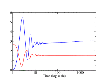
Figure 1: From top (red) to bottom (blue), expectation values of ${\cal O}_{h}^{(6)}$, $K$, and ${\cal N}_{1}$, for ${h=0.3}$ with $N=15$ and $vol({\cal E})\approx 10^{3}$. In the log coordinate $t=\log s$, the approach to the equilibrium is $\langle{\cal O}\rangle(t)-{\cal O}_{\infty}=d/s^{\tau}$ with $d>0$ for ${\cal O}_{h}^{(6)}$ and $d<0$ for $K$.

At the initial time $\langle{\cal O}_{s}^{(6)}\rangle=0$, and $\langle K\rangle$ coincides with (43). The late time behavior of these two observables fits into the ansatz,

$$\langle{\cal O}\rangle(t)={\cal O}_{\infty}+d\,e^{-t/\tau},\quad{\cal O}=K,\,{\cal O}_{s}^{(6)}\,,$$ (63)

with $\tau\approx 700$ in units of time. The dependence of $\tau$ as function of $h$ can be inferred by dimensional analysis. The scaling we should keep in mind is

$$t\rightarrow\lambda^{-1}t\,,\qquad\{\mathfrak{m},X_{I}\}\rightarrow\lambda\{\mathfrak{m},X_{I}\}\leavevmode\nobreak\ .$$ (64)

In the case $\mathfrak{m}=0$, we deduce immediately that $\tau h^{1/4}=C(N)$, where $C$ is a dimensionless constant which only depends on $N$. When the mass is non vanishing, another dimensionless ratio can be considered. In this case the right parametrization is

$$\tau h^{1/4}=\Big{[}C(N)+f\left(\frac{\mathfrak{m}}{h^{\,1/4}},N\right)\Big{]}\leavevmode\nobreak\ ,$$ (65)

with $f$ a function such that $f\rightarrow 0$ as $h^{1/4}\gg\mathfrak{m}$. The same scaling argument can be used to infer the expectation value at the equilibrium of any observable ${\cal O}$ of dimension $\delta$, as function of $h$ and $\mathfrak{m}$:

$$\langle{\cal O}\rangle=h^{\delta/4}\Big{[}C(N)+f\left(\frac{\mathfrak{m}}{h^{\,1/4}},N\right)\Big{]}\leavevmode\nobreak\ .$$ (66)

Both these formulae contain implicitly the assumption that the system equilibrates. We observed experimentally that the regimes of applicability are two:

1. the asymptotic regime $h^{1/4}\gg\mathfrak{m}$;

2. the intermediate regime $h^{1/4}\sim\mathfrak{m}$.

In the first case the dynamics tends to the BFSS matrix model because as $h\rightarrow\infty$ the mass term in the BMN Lagrangian is negligible. In the second case instead, corrections due to the mass term become important. The case $h^{1/4}\ll\mathfrak{m}$ is more complicated, since the mass term are not suppressed, and the time evolution could be comparable to that of harmonic oscillator (possibly for a time longer than our simulation time). In the next sections we will consider numerical simulations in which either 1) or 2) are valid.

The time evolution of the $\langle{\cal O}_{s}^{(3)}\rangle$ singlet is similar to that of $\langle{\cal O}_{s}^{(6)}\rangle$. The trivial result $\langle{\cal N}_{1}\rangle=0$, also shown in Figure 1, was expected. Indeed, the time evolution commutes with the action of the global symmetries, and since the initial data at the big-bang are determined by a single gaussian, $\mathcal{E}_{h}$ is symmetric under $SO(3)\times SO(6)$. It follows that for any configuration $\mathcal{X}\in\mathcal{E}_{h}$, and group element $g$, the ‘rotated’ configuration $g\cdot\mathcal{X}$ also belongs to $\mathcal{E}_{h}$, therefore, the expectation value of any charged observable vanishes. The results obtained so far extend in different directions those obtained in Asplund:2011qj ; Asplund:2012tg .

IV.1 Equilibration and Chaos

Some initial conditions do not lead the system to a late time equilibrium. For example, the expectation value of any observable evaluated on the solutions (46) is obviously periodic in time. Thus, the process of equilibration must be triggered by the non-commutative interaction in the Lagrangian. However, this microscopic feature of the system cannot by itself explain the statistical equilibration of the expectation values of the observables, which is instead a collective phenomena. As we are going to see, chaos is the key towards our understanding of the process of equilibration.

In order to relate chaos and equilibration, we have to discuss an important point. On one hand, the BMN Hamiltonian is non dissipative, and any configuration in the ensemble will keep evolving under time evolution. On the other hand, the expectation value of the observables becomes time independent at late times. It is useful to resolve this apparent logical difficulty by first considering a simpler situation: We may decide to calculate

$$\langle\mathcal{O}\rangle_{0}=\frac{1}{vol(S)}\int_{S}d\mu\ \mathcal{O}(\{\vec{p}_{m}\},\{\vec{x}_{m}\})\leavevmode\nobreak\ ,$$ (67)

where $S$ is the submanifold in phase space allowed by the conserved charges, and $d\mu$ is the flow-preserving volume form on $S$. Acting with $\varphi_{t}$ on $S$ we may calculate as well

$$\langle\mathcal{O}\rangle_{t}=\frac{1}{vol(\varphi_{t}(S))}\int_{\varphi_{t}(S)}d\mu\ \mathcal{O}(\{\vec{p}_{m}\},\{\vec{x}_{m}\})\leavevmode\nobreak\ .$$ (68)

Even though the flow will move any single point in $S$, because $\varphi_{t}(S)=S$, we conclude that $\langle\mathcal{O}\rangle_{t}=\langle\mathcal{O}\rangle_{0}$, and therefore $\langle\mathcal{O}\rangle$ is at the equilibrium. The same conclusion would still hold true, if instead of $S$, we consider a region $\mathcal{A}$ dense in $S$, and we assume the flow to be such that for any $t\geq t_{eq}$ the set $\varphi_{t}(\mathcal{A})$ is uniformly distributed in $S$. In the most general situation, equilibration takes place under the weaker condition that $\varphi_{t}(\mathcal{A})$ at late times defines a probability distribution which is time independent. This distribution, called $\mathscr{P}_{t}$ hereafter, is obtained in the statistical sense by taking the continuum limit in the volume of $\mathcal{E}$ at fixed time, i.e.

$$\frac{1}{vol(\mathcal{E}(t))}\sum_{\mathcal{X}\in\,\mathcal{E}}{\cal O}(\mathcal{X})\rightarrow$$

$$\rule{28.45274pt}{0.0pt}\int_{S}d\mu\,\mathscr{P}_{t}(\{\vec{p}_{m}\},\{\vec{x}_{m}\})\ {\cal O}(\{\vec{p}_{m}\},\{\vec{x}_{m}\})\,.$$ (69)

It is therefore well defined both for small and large-N. The case of an uniform $\mathscr{P}_{t}$ at the equilibrium is the case we mentioned in the example given above.

In our finite $N$ simulations, we should also bear in mind another detail: The fluid, ${\cal E}_{h}(t)$, is not restricted to a single submanifold $S$ but covers the set $\cup_{\gamma}S_{{\cal H}}$ where ${\cal H}$ is the energy of a single configuration in the ensemble. In fact, the energy of the ensemble is a gaussian variable with mean $\langle E\rangle=h\,n_{tot}$ and standard deviation $\sqrt{2}\,\langle E\rangle/\sqrt{n_{tot}(N^{2}-1)}$, as shown in (43).

The property we have invoked about the flow is very much related to the definition of Lyapunov chaos NoteLyapu . An Hamiltonian flow $\varphi$ is said to be chaotic in the sense of Lyapunov if two properties hold:

1. $\varphi_{t}$ is almost everywhere expansive,

2. under time evolution $\varphi_{t}(p)$ visits almost every point in $S$, i.e. $\varphi_{t}$ is topological transitivity.

In particular, the well known Lyapunov exponent $\lambda_{Lya}$ quantifies how much $\varphi_{t}$ is expansive. We have measured $\lambda_{Lya}$ in our simulations, by using the strategy outlined in Gur-Ari:2015rcq , for the BFSS matrix model. Within error we obtain the same result: $\lambda_{Lya}\approx 0.29+O(1/N)$. Even though the ensemble $\mathcal{E}(0)$ was gaussian and localized in phase space, as a consequence of the expansive nature of the flow, $\varphi_{t}(\mathcal{E}(0))$ populates the allowed phase at late times. This is an important feature of the dynamics of chaotic systems as opposed to that of integrable systems. In fact, by taking a constant distribution of initial conditions, it is not difficult to build a fine-tuned equilibration even for the harmonic oscillator. However, this type of equilibration is non generic and will fail upon specifying a different set of initial conditions. In this sense, equilibration for chaotic systems is generic for any given initial conditions.

IV.2 Dynamics of Eigenvalues

Building on our previous remarks about the dynamics of observables of the type

$${\cal O}=\sum_{I}c_{I}\,{\rm{Tr}}(\,f_{I}(X_{I}))\,,\qquad c_{I}\in\mathbb{R}\leavevmode\nobreak\ ,$$ (70)

we can re-express the expectation value of these observables as the integral

$$\langle{\cal O}\rangle=\int\prod_{I=1}^{N}d\lambda^{J}_{\alpha}\ \mathscr{P}^{eig}(\{\lambda^{J}_{\alpha}\})\,\sum_{I,\alpha}c_{I}f_{I}(\lambda^{I}_{\alpha})\leavevmode\nobreak\ ,$$ (71)

where $\alpha=1,\ldots N,$ and $\mathscr{P}^{eig}(\{\lambda_{\alpha}^{J}\})$ is the joint probability distribution of all the eigenvalues of the matrices $\{X_{I}\}$. The summation over the indexes $I$ and $\alpha$ can be brought outside the sign of integration, and the expectation value in (71) is then determined only from the knowledge of the mean eigenvalue density $\rho_{I}^{eig}(\lambda)$ of the $I$-th matrix. This density is obtained by integrating both the set of $\{\lambda^{\alpha}_{J}\}$ with $I\neq J$ and the set of $N-1$ eigenvalues in $\{\lambda^{\alpha}_{I}\}$. Assuming the existence of an equilibrium, the $SO(3)$ and $SO(6)$ symmetries of the ensemble $\mathcal{E}(t)$ imply the relations

$$\rho^{eig}_{i}(\lambda)=\rho^{eig}_{j}(\lambda)\,,\qquad\rho^{eig}_{a}(\lambda)=\rho^{eig}_{b}(\lambda)\,,$$ (72)

$\forall\ i,j,a,b,$ so that only two non trivial eigenvalue distributions exists, one for each symmetry group. Accordingly, the charged operators $\mathcal{N}_{i=1,2}$ have vanishing expectation values. In the BFSS model the symmetry group is enhanced to $SO(9)$ and we would find in addition that ${\rho}^{eig}_{i}={\rho}^{eig}_{a}\$ $\forall\ i,a$. In the BMN model $\mathfrak{m}\neq 0$, and we do not expect this relation to hold. In fact, in the setup of Figure 1, we can explicitly verify that $\langle{\cal O}_{s}^{(6)}\rangle\neq 2\langle{\cal O}_{s}^{(3)}\rangle$.

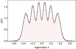
Figure 2: The histogram of the distributions $\rho^{eig}$ in the $SO(6)$ sector for $N=6$ (top) and $h=0.3$. The solid black line is the matched TGU distribution. $vol({\cal E})\approx 10^{5}$.

The histogram of $\rho^{eig}(\lambda)$ in the $SO(6)$ sector for $N=6$ and $\mathcal{E}_{h=0.3}$ is shown in Figure 2. The solid curve is the TGU distribution, which can be computed analitically from the results of TGUexact . The numerical and the TGU distributions agree. For completeness, let us illustrate the analytic calculation: We quote from TGUexact the profile function

$$p_{6}(\lambda) = e^{-\frac{6}{5}\lambda^{2}}\big{(}\begin{array}[]{l}\frac{13436928}{244140625}\lambda^{10}-\frac{4478976}{9765625}\lambda^{8}+\end{array}$$ (76)

$$\rule{0.0pt}{14.22636pt}\rule{2.84544pt}{0.0pt}\begin{array}[]{l}+\frac{2581632}{1953125}\lambda^{6}-\frac{102816}{78125}\lambda^{4}+\frac{7812}{15625}\lambda^{2}+\frac{644}{15625}\end{array}\big{)}\leavevmode\nobreak\ .$$

The distribution $\rho^{eig}_{TGU}(\lambda)$ is proportional to $p_{6}(r\lambda)$, where the parameter $r$ is obtained from the relation

$${\rm{Tr}}(X^{2})=N\int d\lambda\,\lambda^{2}\rho^{eig}_{TGU}(\lambda)\leavevmode\nobreak\ .$$ (77)

The good agreement between $\rho^{eig}_{TGU}(\lambda)$ and the distribution of eigenvalues of any $X_{I}$ at the equilibrium should not be confused with the fact that the ensemble at the equilibrium is TGU. In fact, as a consequence of the non trivial dynamics, the matrices are correlated, and the joint probability distribution does not factorize, i.e. $\mathcal{P}(\vec{x}_{m},\vec{y}_{n})\neq\mathcal{P}(\vec{x}_{m})\mathcal{P}(\vec{y}_{n})$. A simple convincing argument is the following: Let us assume that $Z_{1}$ and $Z_{2}$ are uncorrelated and TGU with variance $\sigma$. Then

$$\langle{\rm{Tr}}(Z_{i}^{2})\rangle_{TGU} = \,{(N^{2}-1)}(2\sigma^{2})\,,$$ (78)

$$\langle\mathcal{C}_{4}[Z_{1},Z_{2}]\,\overline{\mathcal{C}}_{4}[Z_{1},Z_{2}]\rangle_{TGU} = 8(N^{2}-1)(4\sigma^{4})\,,$$ (79)

and we obtain the exact relation, ${\cal Y}[Z_{1},Z_{2}]_{TGU}=1$, where,

$${\cal Y}[Z_{1},Z_{2}]\equiv\frac{N^{2}-1}{8}\frac{\langle\mathcal{C}_{4}[Z_{1},Z_{2}]\overline{\mathcal{C}}_{4}[Z_{1},Z_{2}],\rangle}{\langle{\rm{Tr}}(Z_{1}^{2})\rangle\langle{\rm{Tr}}(Z_{2}^{2})\rangle}\leavevmode\nobreak\ .$$ (80)

The presence of dynamical correlations in ${\cal E}_{h}(t)$ at the equilibrium can be detected by studying, for example, the time evolution of ${\cal Y}[X_{3},X_{4}]$. In the top panel of Figure 3 we have plotted the expectation value of this observable for $\mathcal{E}_{h=0.3}$ and $N=10$. At the equilibrium, ${\cal Y}[X_{3},X_{4}]$ deviates considerably from unity, and we conclude that $\mathcal{E}(t)$ is not TGU. Since the approach to the equilibrium is exponentially fast, the result is robust. From dimensional analysis we know that the value of ${\cal Y}[X_{3},X_{4}]$ at the equilibrium (hereafter ${\cal Y}_{eq}$) is a function of $N$ and $\mathfrak{m}/h^{1/4}$. In particular, as $h$ is increased, we expect to recover the result at $\mathfrak{m}=0$ (which is $h$ independent). From our simulations we are able to confirm the correctness of this argument. In fact, starting from the result of Figure 3, where ${\cal Y}_{eq}\approx 1.19$ for $h=0.3$, we have tested the converge of ${\cal Y}_{eq}$ measuring ${\cal Y}_{eq}\approx 1.26$ for $h=38.4$, and ${\cal Y}_{eq}\approx 1.31$ at $\mathfrak{m}=0$.

Differently from the $X_{I}$, we can shown that the momenta belong to a TGU ensemble. This can be inferred from the bottom panel of Figure 3, where we have measured ${\cal Y}[P_{3},P_{4}]$. At late times, ${\cal Y}[P_{3},P_{4}]-1$ is zero within the error. Notice that at very early times instead, the time evolution of the coordinates is driven by that of the the momenta, and since the latter are initiated as TGU, the value of ${\cal Y}[X_{3},X_{4}]$ is still close to unity as long as the non-commutative interactions can be neglected.

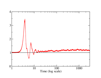
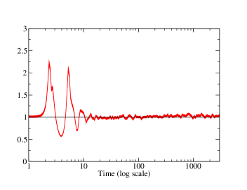
Figure 3: Time evolution of ${\cal Y}[X_{3},X_{4}]$ (top) and ${\cal Y}[P_{3},P_{4}]$ (bottom) for $N=10$ and $h=0.3$, with $vol({\cal E})\approx 10^{4}$. The solid line ${\cal Y}=1$ is the TGU result.

V IV.  Dynamical Relaxation

The aim of this section is to study the close-to-the equilibrium relaxation of the observables. In order to do so, we devise a quench protocol that takes $\mathcal{E}_{h}(t)$ at the equilibrium, and push it onto a phase space region whose distance from $\mathcal{E}_{h}(t)$ can be tuned in a controlled way. We define the notion of distance between two ensembles by measuring the differences between the conserved charges. By assuming that the level sets of the conserved charges change in a smooth way, a given quench will generate a close-to-equilibrium configuration when the variation of the conserved charges before and after the quench is small. Instead, the quench will generate a far-from-equilibrium configuration when the conserved charges are changed abruptly. As we are going to show, our results will indeed confirm this phase space picture.

V.1 Quench Protocol

Let us begin by describing our three-steps protocol:

1. From the initial big-bang we wait until the system equilibrates, say at time $t_{quench}$.
   

2. We perform a global gauge transformation with an unitary matrix $U$ on (the history of) any configuration $\mathcal{X}$, i.e.

   $$X_{I}(t) \rightarrow UX_{I}(t)U^{\dagger}\equiv X_{I}^{(U)}\,,$$ (81)

   $$P_{I}(t) \rightarrow UP_{I}(t)U^{\dagger}\equiv P^{(U)}_{I}\,,$$ (82)

   and we choose $U$ such that at $t_{quench}$, and for a given index $\mathfrak{p}$, the matrix $UX_{\mathfrak{p}}U^{\dagger}=D$ is diagonal;

3. For any $D$, we order the eigenvalues of $D={\rm diag}(\lambda_{1},\ldots,\lambda_{N})$ from least to greatest, and we perform the shift

   $$D\leavevmode\nobreak\ \rightarrow\leavevmode\nobreak\ \widetilde{D}\equiv D+\mathrm{diag}(\epsilon_{1},\ldots,\epsilon_{N})\leavevmode\nobreak\ ,$$ (83)

   with quench parameters $\epsilon_{\alpha=1,\ldots N}$.

The constraint is not violated if at the same time we perform a deformation of the momentum

$$P^{(U)}_{\mathfrak{p}}\leavevmode\nobreak\ \rightarrow\leavevmode\nobreak\ \widetilde{P}^{(U)}_{\mathfrak{p}}\equiv P^{(U)}_{\mathfrak{p}}+\ \delta[P^{(U)}_{\mathfrak{p}},D]\leavevmode\nobreak\ ,$$ (84)

where the operator $\delta[P,D]$ returns the hermitian matrix which solves the matching condition,

$$\sum_{I}[P^{(U)}_{I},X^{(U)}_{I}]=\sum_{I\neq\mathfrak{p}}[P^{(U)}_{I},X^{(U)}_{I}]+[\widetilde{P}^{(U)}_{\mathfrak{p}},\widetilde{D}\,]\leavevmode\nobreak\ .$$ (85)

The traceless condition of $\widetilde{D}$ is achieved by considering quench parameters which add up to zero. The traceless condition is automatic in $\delta[P,D]$ because its diagonal elements do not play a role in solving (85), and therefore can be chosen arbitrarily. The complete solution of $\delta[P,D]$ is not illuminating, instead we shall mention two interesting cases which we use in our numerical simulations:

• Consider perturbing the edge of $D$ by taking $\epsilon_{1}=-\epsilon=-\epsilon_{N}$ and $\epsilon_{\alpha}=0$ for $\alpha\neq\{1,N\}$. The corresponding $\delta[P,D]$ returns an hermitian matrix whose entries are all zero but,

  $$(\delta[P,D])_{1m}\,= -\frac{\epsilon\leavevmode\nobreak\ (P)_{1m}}{\epsilon-(D)_{11}+(D)_{mm}} \quad 2\leq m<N$$

  $$(\delta[P,D])_{1N}\,= -\frac{2\epsilon\leavevmode\nobreak\ (P)_{1N}}{2\epsilon-(D)_{11}+(D)_{NN}}$$ (86)

  $$(\delta[P,D])_{mN}= -\frac{\epsilon\leavevmode\nobreak\ (P)_{mM}}{\epsilon-(D)_{mm}+(D)_{NN}} \quad 2\leq m<N\leavevmode\nobreak\ .$$

  Let us notice that in order for this deformation to actually take place as $N\rightarrow\infty$, it may be necessary to consider,

  $$\widetilde{D}\equiv D+\mathrm{diag}(\underbrace{-\epsilon_{1},..,-\epsilon_{k}},0,..,0,\underbrace{+\epsilon_{k},..,+\epsilon_{1}})\,,$$ (87)

  while keeping $k/N$ fixed. It is worth emphasizing at this point, that the quench is not symmetric under $\epsilon\rightarrow-\epsilon$. This can be understood by considering the denominators of $\delta[P,D]$. For example, the quantity $-(D_{11}-\epsilon)+D_{22}$ depends on both the sign of $\epsilon$, and the difference between two near-neighbour eigenvalues of $\widetilde{D}$. For one sign $\epsilon$, there exists a small value of $-\epsilon$ for which the denominator diverges, and as a result, we expect the quenched configuration to be a far-from-equilibrium configuration.

• Consider a quench in which $D$ is inflated. This configuration is achieved by defining $\epsilon_{\alpha}=\lambda_{\alpha}\overline{\epsilon}$, with a given $\overline{\epsilon}$. In matrix notation

  $$\widetilde{D}=(1+\overline{\epsilon})D\leavevmode\nobreak\ .$$ (88)

  Notice that the traceless condition is automatically satisfied. The solution of $\delta[D,P]$ also takes a very simple form, in particular the quench along the momentum reduces to $\widetilde{P}^{(U)}_{\mathfrak{p}}=(1+\epsilon)^{-1}{P}_{\mathfrak{p}}^{(U)}$. Again the traceless condition is automatically satisfied.

Finally, we remark that $A_{t}=0$ remains solution after the quench.

V.2 Features of the Quenched Ensemble

The outcome of the quench protocol is an initial condition for a new ensemble $\mathcal{E}^{\prime}$, which depends explicitly on the quench parameters and implicitly on $h$. This new ensemble will evolve on a sub-manifold of the phase space which is not that of $\mathcal{E}_{h}$. As we mentioned, the notion of “distance” between ensembles is better quantified by looking at the variation of the conserved charges. For example, if we consider an edge-type quench we should calculate the expectation value of the following quantities,

$$\Delta{\rm{Tr}}(X_{\mathfrak{p}}P^{I})=\epsilon(P^{I}_{NN}-P^{I}_{11})\,,$$ (89)

$$\Delta{\rm{Tr}}(P_{\mathfrak{p}}X^{I})=\begin{array}[]{l}\sum_{m\leq N}\mathrm{Re}(\delta[P_{\mathfrak{p}},D]_{1m}X^{I}_{m1})\ +\end{array}\rule{0.0pt}{14.22636pt}$$ (91)

$$\rule{56.9055pt}{0.0pt}\begin{array}[]{l}+\sum_{m<N}\mathrm{Re}(\delta[P_{\mathfrak{p}},D]_{Nm}X^{I}_{mN})\leavevmode\nobreak\ .\end{array}\rule{0.0pt}{11.38092pt}$$ (93)

Since we are especially interested in generating close-to-equilibrium initial conditions, we will tune the quench parameters in such a way that the conserved charges admit a perturbative expansion. Even in this regime, it is highly non trivial to compute their expectation value analytically. Nevertheless, simple arguments based on dimensional analysis and the scaling law (64) provide us with the right parametrization in terms of $\epsilon$ and $h$. Continuing with edge-type quenches, the variation of the energy $\Delta\langle E\rangle=9h-{\cal H}(\mathcal{E}^{\prime})$ is then

$$\frac{\Delta\langle E\rangle}{9h} = 1+\frac{\epsilon}{h^{1/4}}f\left(\frac{\mathfrak{m}}{h^{1/4}},N\right)+O(\epsilon^{2})\,,$$ (94)

$$f = c_{0}+c_{1}\frac{\mathfrak{m}}{h^{1/4}}+c_{2}\frac{\mathfrak{m}^{2}}{h^{1/2}}+\ldots\,,$$

where the $c_{i}$ only depend on $N$. This is the most general expression compatible with both the scalings $h\rightarrow\lambda^{4}h$, $\epsilon\rightarrow\lambda\epsilon$, and the limit $\epsilon\rightarrow 0$. For the BFSS matrix model, the conserved quantities will only depend on $\epsilon/h^{1/4}$, but in the generic case there are other contributions in $h$ as long as $h/\mathfrak{m}\sim 1$. Arguments based on dimensional analysis are also valid for inflation-type quenches, the only difference to bear in mind is that $\overline{\epsilon}$ now plays the role of $\epsilon/h^{1/4}$. Some formulae simplify. For example, the order $\overline{\epsilon}$ in the $\langle E\rangle$ is

$$\frac{\Delta\langle E\rangle}{9h} = 1+\overline{\epsilon}\ \langle{\rm{Tr}}(G_{\mathfrak{p}})\rangle+O\big{(}\overline{\epsilon}^{2}\,\big{)}\,,$$

$$G_{\mathfrak{p}} = -P_{\mathfrak{p}}^{2}-\sum_{J}[X_{\mathfrak{p}},X_{J}]^{2}+m^{2}X_{\mathfrak{p}}^{2}\,,$$ (95)

where $m$ depends on whether $\mathfrak{p}\in\{a,i\}$, according to (6) or (9). $G_{\mathfrak{p}}$ represents the difference between kinetic and potential energy of the configurations $(P_{\mathfrak{p}},X_{\mathfrak{p}})$. As expected from considerations about the equipartition theorem, we checked that $G_{\mathfrak{p}}$ vanishes. Therefore, $\Delta\langle E\rangle$ is at least quadratic in $\overline{\epsilon}$ for inflation-type of quenches.

A more concrete way of understanding how the quench acts on the ensemble is to consider its consequences on the dynamics of the observables we are interested in. According to our previous discussion, from the knowledge of the distribution of eigenvalues $\rho^{eig}_{I}$ of each matrix $X_{I}$, we completely determine the expectation value of observables of the type ${\cal O}={\rm{Tr}}({\cal M})$, where

$${\cal M}[\{X_{I}\}]=\sum_{I}c_{I}f_{I}(X_{I})\,,\qquad c_{I}\in\mathbb{R}\leavevmode\nobreak\ .$$ (96)

Deforming one of these distributions is precisely the task of the quench protocol. In fact, by rotating $X_{\mathfrak{p}}$, we obtain $N$ eigenvalues extracted from $\rho^{eig}_{\mathfrak{p}}$ at the equilibrium, and by shifting $D$ to $\widetilde{D}$, in practice, we deform $\rho^{eig}_{\mathfrak{p}}$ by changing its support. Therefore, a mismatch of the same order of magnitude of the quench parameters exists between the the shape of the distribution at $t^{+}_{quench}$ and that of the equilibrium distribution at $t^{-}_{quench}$. This picture is particularly helpful if we want to visualize in which way $\mathcal{E}^{\prime}$ represents a close-to-equilibrium initial condition from the point of view of the observable.

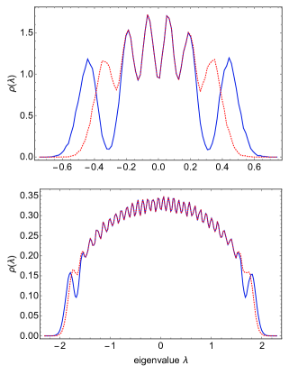
Figure 4: Top panel: The distribution $\rho^{eig}_{\mathfrak{p}=4}$ at $t^{-}_{quench}$ (dotted red curve) and at $t^{+}_{quench}$ (solid blue curve), for $N=6$, $h=0.3$ and quench parameter $\epsilon=0.1$. Bottom panel: Same as above with $N=30$, $\sigma=1/8$ and $\epsilon=0.05$.

In Figure 4 we compare the distribution just before and after the quench time for edge-type quenches. For any value of $N$, the equilibrium distribution in $\mathcal{E}$ is characterized by $N$ distinct peaks. For small $N$ the picture is simpler. At $t^{+}_{quench}$, we find that the position of the peaks at the edge of the distribution has moved from the inside out of order $\epsilon$, whereas the bulk of the distribution has remained almost unchanged. Since the number of peaks increases with $N$, the same logic goes through. We may get a feeling about the large-N result by repeating the quench protocol in the case of a TGU matrix. As Figure 4 shows, the outcome of the quench produces a ripple in the equilibrium distribution.

For each event in $\mathcal{E}^{\prime}$ the $SO(3)\times SO(6)$ symmetry is broken to the subgroup of rotations that leave $X_{\mathfrak{p}}$ fixed. The breaking is explicit, and the full symmetry is not restored on the ensemble since the direction of the broken charges is the same for all configurations. Thus, if $\mathfrak{p}\in\{1,2,3\}$ (or $\mathfrak{p}\in\{4,\ldots,9\}$) $\mathcal{E}^{\prime}$ preserves $SO(2)\times SO(6)$ (or $SO(3)\times SO(5)$). After reaching the new equilibrium in $\mathcal{E}^{\prime}$, we expect the set of $\rho^{eig}_{I}$ with $I\neq\mathfrak{p}$ to be equal, according to the preserved symmetries, whereas the distribution $\rho^{eig}_{\mathfrak{p}}$ to be different in a way which is determined by the strength of the quench parameter. Given the asymmetry in the eigenvalues distributions, the charged operators ${\cal N}_{i=1,2}$ will acquire a non trivial expectation value. In the next section we will study the time evolution of these operators for close-to-equilibrium quenches. Some examples of edge-type quenches in which $\epsilon\gg 1$ are illustrated in Appendix B.

V.3 Quasi-Normal Modes

The time evolution of the observables after the quench has some notable features. In the top panel of Figure 5 we have plotted the expectation value of ${\cal N}_{2}$, from the quench to the new equilibration. Two facts show up clearly:

1. $\langle{\cal N}_{2}\rangle$ relaxes fast, without experiencing any non linear transition typical of the big-bang.

2. The process of relaxation is driven by quasi-normal oscillations. These modes are collective excitations of the non-commutative dynamics.

Before discussing which ansatz describes the quasi-normal ringing, it is interesting to ask how we should think about these oscillations in phase space. Let us consider that at the equilibrium $\mathcal{E}(t)$ is described by a distribution $\rho_{t}$ which does not change in time, so intuitively, any realization of $\mathcal{E}(t)$ covers the support of this distribution with the correct weight. As we pointed out, the equilibrium distribution after the quench has moved to a different support, and evidently $\mathcal{E}^{\prime}(t^{+}_{quench})$ does not cover enough of it. Under the assumption that $\mathcal{E}^{\prime}(t^{+}_{quench})$ is a close-to-equilibrium initial conditions, we expect the holes between $\mathcal{E}^{\prime}(t^{+}_{quench})$ and the support of the new equilibrium distribution, to populate quickly. During this process the dynamics of the observables is driven by quasi-normal oscillations. The ring-down of the observables is in one-to-one correspondence with the ring-down of the distribution of eigenvalues, since both are functions of the microscopic degrees of freedom.

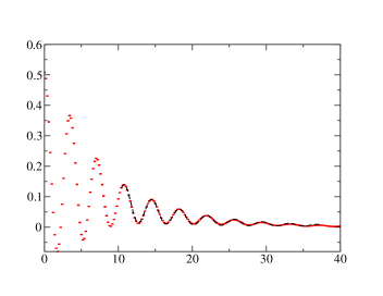
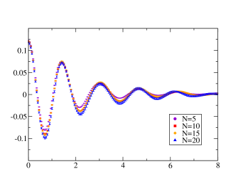
Figure 5: Top panel: The behavior of $\langle{\cal N}_{2}\rangle(t-t_{quench})$ for an edge-type quench, with $h=0.6$, $\epsilon=0.25$, and $N=15$. The solid curve is the lowest quasinormal mode obtained from our fit procedure. Bottom panel: The behavior of $\langle{\cal N}_{2}\rangle(t-t_{quench})$ for an inflation-type quench, various values of $N$, $\mathfrak{h}=0.1$, and $\overline{\epsilon}N=0.06$.

The behavior of the $\langle{\cal O}\rangle(t)$ after the quench is a superposition of quasi-normal modes. Close to the new equilibrium, the lowest quasi-normal mode is the dominant one, and the behavior of the observable is fitted into the following ansatz,

$$\langle{\cal O}\rangle(t)={\cal O}_{\infty}+e^{-t/\tau}\Big{(}d+u\cos(\Omega t+\phi)\Big{)}\,,$$ (97)

where ${\cal O}$ stands for any of the observables we are considering. The details of the fitting procedure are reported in the Appendix A. Here, $\tau^{-1}$ and $\Omega$ are the damping and the ringing frequencies, respectively. In complex notation, it is convenient to define $\omega\equiv\Omega-i\tau^{-1}$. Tuning the values of $d$ and $u$, the ansatz accommodates both an over- and an under-damping behavior. It is important to emphasize that the quenched ensemble, by construction, has different properties compared to $\mathcal{E}_{h}$. In particular, we expect $d$, $u$ and ${\cal O}_{\infty}$ to be directly proportionals to the quench parameters because of the explicit symmetry breaking. Since we are interested in studying the fluctuations of the equilibrium distribution in $\mathcal{E}_{h}$, we will consider the limit $\epsilon\rightarrow 0$, for edge-type quenches, and $\overline{\epsilon}\rightarrow 0$ for inflation-type quenches. The only quantities whose limiting values will be non trivial are the frequencies $\tau^{-1}$ and $\Omega$.

Once again, dimensional analysis provides us with the basic tools to understand the data. The complex frequency can be parametrized as,

$$\omega = h^{1/4}\Big{[}c_{0}(N)+f\left(\frac{\mathfrak{m}}{h^{\,1/4}},N\right)\Big{]}\,,$$ (98)

where $c_{0}$ is coefficients, and $f$ is a function which vanish in the asymptotic regime. The limit $h^{1/4}\gg\mathfrak{m}$ is very useful here, because as long as the mass parameter is irrelevant the BFSS and the BMN model have a similar dynamics. On one hand, we are free to study the BFSS model independently, setting $\mathfrak{m}=0$, with the advantage that the model has a simpler dynamics. On the other hand, we can check that the values of $\omega$, taken from the BMN model, asymptote those of BFSS model. Comparing the results of BFSS simulations at $N=10,15,20$, within error we find the relation

$$\omega\propto\ \mathfrak{h}^{\frac{1}{4}}\,,\quad\mathfrak{h}\equiv\frac{h}{N}\leavevmode\nobreak\ .$$ (99)

We conclude that in the asymptotic regime, the natural variable upon which $\omega$ and $\tau$ depend is $h/N$. We should mention that at smaller values of $N$, for example $N=5,6$, we have measured small deviations from the scaling regime (99). On the other hand, the dependence on $\mathfrak{h}$ can be understood as follows: In the large-N limit we would find the relation $h/N=\int\rho(\lambda_{\mathcal{H}})\lambda_{\mathcal{H}}$, where $\rho$ is the distribution of eigenvalues of the BMN Hamiltonian $\mathcal{H}$. Therefore, in order to have a well defined energy distribution we should keep $h/N$ fixed.

The scaling with $N$ actually holds for the entire profile of the quasi-normal oscillation. This is shown in the bottom panel of Figure 5, where we have plotted the behavior of $\langle\mathcal{N}_{2}\rangle(t)$ for inflation-type quenches by keeping $\mathfrak{h}$ and $N\overline{\epsilon}$ fixed. The latter condition follows from the observation that

$$\langle{\rm{Tr}}\,X_{I}^{2}\rangle\propto\sqrt{Nh}\leavevmode\nobreak\ .$$ (100)

Within error we cannot appreciate any difference on $\langle\mathcal{N}_{2}\rangle(t)$ among $N=10,15,20$, and the deviations visible at $N=5$ can be addressed to $1/N$ corrections.

Outside the asymptotic regime, corrections due to the mass $\mathfrak{m}$ cannot be neglected, and we expect them to organize in a series expansion of the form

$$f=c_{1}(N)\left[\,\frac{\mathfrak{m}^{4}}{\mathfrak{h}\,}\right]^{p}+{\rm higher\ order\ terms}\,,$$ (101)

where $p$ and $c_{1}$ need to be determined. We have found that $p=1/2$ and $c_{1}$ is, within error, an $N$ independent constant. In Figure 6 we have plotted $\omega\mathfrak{h}^{-1/4}$ as function of $\mathfrak{m}^{2}/\mathfrak{h}^{1/2}$. We can fit these two curves with the ansatz,

$$\omega\,\mathfrak{h}^{-1/4} = c_{0}+c_{1}\left[\,\frac{\mathfrak{m}^{4}}{\mathfrak{h}\,}\right]^{{1}/{2}}+c_{2}\left[\,\frac{\mathfrak{m}^{4}}{\mathfrak{h}\,}\right]\,,$$ (102)

with coefficients:

$$c_{0} =3.407(10)-i\,0.435(12)\,,$$

$$c_{1} =0.0543(30)+i\,0.0291(32)\,,$$

$$c_{2} =0.00138(20)-i\,0.00097(20)\leavevmode\nobreak\ .$$ (103)

It is worth mentioning that the numerical fit of (102) do not depend on the details of the quench protocol, in particular we do not find differences between edge- and inflation-type quenches when we look at the curves of $\omega\,\mathfrak{h}^{-1/4}$. In the linear response regime, this is a consequence of the fact that the location of the poles of the Green functions are independent of the strength of the perturbation.

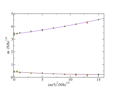
Figure 6: The curves of $\omega$ for the lowest quasinormal mode of $\mathcal{E}_{h}$, obtained from inflation-type quenches. The parametrization of the axis is explained in the main text. The color code is black $N=10$, red $N=15$, green $N=20$. (Data have been slightly shifted horizontally to improve the readability).

VI V. ${\cal N}=4$ SYM on $\mathbb{R}\times\mathbb{S}^{3}$

The BMN matrix model can be understood as a classical (supersymmetric) consistent truncation of $\mathcal{N}=4$ SYM on $\mathbb{R}\times\mathbb{S}^{3}$. This connection was established in Kim:2003rza , where the authors showed that the equations of motions of the $\mathcal{N}=4$ gauge multiplet $(A_{\mu},\chi^{A=1,\ldots,4}_{\alpha},\phi^{i=4,\ldots,9})$, truncated to the lowest harmonics of $\mathbb{S}^{3}$, reduce to those of the BMN matrix model. The details of the truncation are as follows,

$$\phi^{i} = \overline{X}^{i}(t)\,,\quad A_{t}=A_{t}(t)\,,$$ (104)

$$A_{\mu=\{\theta,\varphi,\psi\}} = \sum_{c=1}^{3}\overline{X}_{c}(t){\bf V}^{c+}_{\mu}({\bf x})\,,$$ (105)

$$\chi_{\alpha}^{A} = \sum_{\alpha=1}^{2}\theta^{A}_{\beta}(t){\bf S}^{\beta+}_{\alpha}({\bf x})\,,$$ (106)

where $\overline{X}^{i}\oplus{\bf V}^{c+}\oplus{\bf S}^{\beta+}$ span the irrep $(1,1,6)\oplus(3,1,1)\oplus(2,1,4)$ of the $SU(2)_{+}\otimes SU(2)_{-}\otimes SU(4)_{R}$ symmetry group. In (1) we considered only the scalar sector of this truncation, setting the fermions $\theta^{A}_{\beta}$ to zero, and redefining the radius ${\mathsf{R}}$ of the $\mathbb{S}^{3}$ as $\mathfrak{m}=6/{\mathsf{R}}$. Recalling that the covariant derivatives acting on the gauge multiplet are $D_{\mu}=\nabla_{\mu}-ig_{YM}A\wedge$ and $F=dA-ig_{YM}A\wedge A$, and the quartic coupling is $g^{2}_{YM}[\overline{X}_{I},\overline{X}_{J}]^{2}$, we obtain the BMN action by considering the field redefinition $\overline{X}=X/g_{YM}$. The final result is

$$\SS_{\mathcal{N}=4}^{truncated}=\frac{\,vol(\mathbb{S}^{3})}{g_{YM}^{2}}\SS_{BMN}[\{X_{I}\},A_{t}]\leavevmode\nobreak\ .$$ (107)

In the regime where $g^{2}_{YM}\ll 1$ and $\overline{X}g_{YM}$ is kept fixed, the classical saddle point approximation is justified, and the study of the BMN matrix model carried out throughout sections I-IV can be reinterpreted as the study of $\mathcal{N}=4$ SYM in the BMN truncation in the classical limit. The only change we need to implement is to redefine the energy as:

$$\mathsf{E}=\frac{vol(\mathbb{S}^{3})}{g^{2}_{YM}}\,{\cal H}\,=\frac{9\,vol(\mathbb{S}^{3})}{g^{2}_{YM}}\,h\,,$$ (108)

where ${\cal H}$ is the BMN Hamiltonian (32).

In the gauge theory, the Dyson fluid represents a finite energy ensemble of classical D3-branes in which the off-diagonal modes are fluctuating. Microscopically, the system is non-commutative and non-perturbative with respect to the dynamics of the diagonal degrees of freedom. Therefore, the weak-coupling “geometric” interpretation of the D3-branes has to be rediscovered through the looking glass of the gauge invariant operators of $\mathcal{N}=4$ SYM. In particular, a “geometric” picture should emerge from the description of the system offered by the eigenvalue distributions associated to each single trace operators. This picture is inspired by the AdS/CFT correspondence which, in the regime of strong ’t Hooft coupling, relates the dynamics of field configurations to those of a gravitational problem in the Anti-de-Sitter space. Being aware that a direct comparison between AdS physics and our Dyson fluid would not be possible, we find important to study the two dynamics in a non trivial case, precisely with the aim of highlighting the major differences.

In the following we review basic aspects of the AdS/CFT correspondence, and we will compute quasi-normal modes for the dual operators that we studied in the BMN truncation. Since at this point we are only interested in qualitative features, we will carry out our toy model computation in a simple black-hole geometry, and we will not go beyond the AdS₅-Schwarzschild black hole.

VI.1 AdS/CFT Correspondence and Black Holes

One of the greatest achievements of string theory has been the discovery of the AdS/CFT correspondence, or more generically, of the gauge/gravity dualities. For $\mathcal{N}=4$ SYM the dual space-time is an asymptotically AdS${}_{5}\times\mathbb{S}^{5}$ background. The two sides of the duality are related by the the D-brane construction of the field theory Maldacena:1997re which sets,

$$L_{\mathbb{S}^{5}}^{4}=L_{AdS_{5}}^{4}=4\pi\alpha^{2}(g_{s}N)\,,\qquad g_{s}=g^{2}_{YM}\,,$$ (109)

where $L_{AdS_{5}}$ and $L_{S^{5}}$ are the radii of AdS${}_{5}\times\mathbb{S}^{5}$, $g_{s}$ is the dimensionless string coupling, and $\alpha$ is the string tension. The radii of AdS₅ and $S^{5}$ are equal and we shall refer to them simply as $L$. The reader unfamiliar with the AdS space might find useful to think about it as a “box” of constant negative curvature proportional to $1/L^{2}$.

The quantity $L^{2}/\alpha$ depends only on the ’t Hooft coupling $\lambda_{t}\equiv g_{YM}^{2}N$. Keeping $\lambda_{t}$ fixed, and taking the large-N limit, the string theory becomes perturbative, i.e. $g_{s}\ll 1$. Then, two cases are well under control:

1. When $\lambda_{t}\gg 1$, the $AdS_{5}\times\mathbb{S}^{5}$ background is classical and the string theory can be truncated to $10d$ classical gravity with Newton constant $G_{10}=8\pi^{6}g_{s}^{2}\alpha^{4}$ D'Hoker:2002aw . In this regime, the duality is very powerful and predicts that $\mathcal{N}=4$ SYM at strong coupling is dual to a gravitational theory in $AdS_{5}\times\mathbb{S}^{5}$. The holographic dictionary provides the concrete link between the two theories Witten:1998qj . In particular, the $4d$ space-time, where the field theory lives, is identified with the boundary of AdS₅, and chiral single-trace operators in the field theory are mapped to bulk fields of the $10d$ geometry. Intuitively, any field configuration at the boundary now acquires a bulk profile along the the fifth (extra) radial coordinate of AdS₅. This bulk profile is obtained by solving classical gravitational equations of motion. The near-boundary behavior of bulk fields plays an important role in the holographic dictionary, and a more precise statement about it will be made in the next section.

2. When $\lambda_{t}\ll 1$ the field theory is perturbative. In this regime the curvature of the gravitational background is large, and the classical spacetime structure has to be modified by quantum gravity corrections.

It is important to realize that according to the basic principles of holography, asymptotically AdS solutions are specified uniquely by the set of conserved charges of the boundary field theory, together with the expectation values of charged operators. These are the same charges we used to initialize and characterize $\mathcal{E}$, as well as more complicated ensembles like $\mathcal{E}^{\prime}$. Therefore, in order to set up a comparison with $\mathcal{E}$, we should at least look for a gravity solution with finite energy, zero momentum, and zero $SO(6)$ charges. Moreover, we should also look for a solution which supports quasinormal oscillations. Together, these two observations point to the simplest and most primitive candidate: the AdS₅-Schwarzschild black hole.

Black holes have special properties: Since the seminal works of Bekenstein, Hawking and Gibbons, it has been recognized that thermodynamic variables can be assigned to stationary black holes Bekenstein:1973ur ; Gibbons:1976ue , and via the AdS/CFT duality it has been understood that an asymptotically AdS black hole corresponds to a field configuration which is approximately thermal. Black holes do not only appear as static objects, but they are also characterized by important dynamical features, in particular by the spectrum of their quasinormal oscillations. In this respect, let us notice that AdS₅ would not have worked for our comparison, simply because at the linearized level it only allows for normal oscillations. By the AdS/CFT duality, the ringing frequency and the decay rate of the lowest quasinormal modes of the black hole control the scales of the process of “thermalization” in the field theory Berti:2009kk .

VI.2 The AdS₅-Schwarzschild black hole

In our notation the AdS₅-Schwarzschild black hole is described by the metric

$$ds^{2}_{BH} = -f(r)dt^{2}+{r^{2}}\,R^{2}d\Omega_{3}^{2}+\frac{dr^{2}}{f(r)}\,,$$ (110)

$$\rule{0.0pt}{14.22636pt}f(r) = \frac{r^{2}}{L^{2}}+\frac{1}{R^{2}}-\frac{ML^{2}}{r^{2}}\leavevmode\nobreak\ .$$ (111)

This background is a solution of the $5d$ Einstein action,

$$I=\frac{1}{16\pi G_{5}}\int\sqrt{g}\ ({\cal R}-\Lambda)+I_{GH}\,,$$ (112)

where $I_{GH}$ is the standard Gibbons-Hawking surface term, and

$$\Lambda=-\frac{12}{L^{2}}\,,\qquad\frac{1}{G_{5}}=\frac{2N^{2}}{\pi L^{3}}\leavevmode\nobreak\ .$$ (113)

The $5d$ Newton constant $G_{5}$ is obtained as the ratio of $G_{10}$ over the volume of the ${\mathbb{S}^{5}}$, which is trivially fibered in the full 10$d$ geometry of string theory. $G_{10}$ has a stringy expression in terms of $\alpha$ D'Hoker:2002aw , thus upon substituting $L$ for $\alpha$, we obtain $G_{5}$ as written in (113).

The radial coordinate $r$ extends from the boundary at infinity, corresponding to $\mathbb{R}\times\mathbb{S}^{3}$, to the radius of the horizon, hereafter $r_{h}$, which is defined as the greatest root of the equation

$$f(r_{h})=\frac{r_{h}^{2}}{L^{2}}+\frac{1}{R^{2}}-\frac{ML^{2}}{r_{h}^{2}}=0\leavevmode\nobreak\ .$$ (114)

The parameter $M$ is called the non-extremality parameter. When $M=0$ the geometry is that of pure $AdS_{5}$ in global coordinates. The radius of the boundary $\mathbb{S}^{3}$ is measured in units of $L$, i.e. $R=\mathsf{R}/L$, where $\mathsf{R}$ is the field theory quantity.

VI.3 Boundary Energy and Thermodynamics

As we mentioned earlier, the mapping between gravitational solutions and field theory configurations goes through the correct identification of the conserved charges on both sides. In our case, the energy. From the bulk perspective, the quantity we need to evaluate is the time component of the stress-energy tensor integrated over the three-sphere at the boundary. This is properly defined as

$$\mathsf{E}=\int d\Omega_{3}\,\sqrt{g}\Big{|}_{\mathbb{S}^{3}}(u^{\mu}\,T^{reg}_{\mu\nu}\,\xi^{\nu})\ \Big{|}_{r=\infty}\,,$$ (115)

where $u^{\mu}=(u^{t},0,0,0,0)$ is the time-like unit vector orthogonal to $\mathbb{S}^{3}$, and $\xi^{\nu}$ is the Killing vector $\sqrt{g_{tt}}\,u^{\mu}$. The stress tensor is

$$T^{ab}=\frac{2}{\sqrt{-h}}\frac{\delta I}{\delta h_{ab}}\,,$$ (116)

where $h_{ab}$ is defined from writing the metric as $ds^{2}_{5}=\mathscr{N}^{2}dr^{2}+h_{ab}(d\sigma^{a}+\mathscr{V}^{a}dr)(d\sigma^{b}+\mathscr{V}^{b}dr)$ (see Liu:2003px for our conventions). The expression of $T^{reg}_{\mu\nu}$ includes counter-terms which regulate well understood divergences in AdS. The result for $T^{reg}_{\mu\nu}$ is

$$T_{tt}^{reg} = \frac{1}{8\pi G_{5}}\frac{3L}{2r^{2}}\left(M+\frac{1}{4R^{4}}\right)\,,$$ (117)

Plugging this expression in (115) and using the relation between $G_{5}$ and $L$, we finally obtain

$${\mathsf{E}} = \frac{3\,vol(\mathbb{S}^{3})}{8\pi^{2}}{}\left(\frac{N^{2}M}{L^{4}}+\frac{N^{2}}{4{\mathsf{R}}^{4}}\right)\,,$$ (118)

where $vol(\mathbb{S}^{3})=2\pi^{2}{\mathsf{R}}^{3}$. The answer for $\mathsf{E}$ is the sum of a zero point (Casimir) energy proportional to $1/{\mathsf{R}}^{4}$ and a physical $M$-dependent energy which can then be rewritten in the form,

$${\mathsf{E}_{phys.}} \equiv \frac{3\,vol(\mathbb{S}^{3})}{8\pi^{2}}{}\frac{NM}{4\pi g^{2}_{YM}}\leavevmode\nobreak\ .$$ (119)

The factors of $g_{YM}^{2}$ and ${vol(\mathbb{S}^{3})}$ in this formula are the same as in the field theory definition of the energy, and the actual value of the energy is proportional to $N$ times $M$. In the field theory ${\mathsf{E}}$ is computed thought the path integral with the insertion of the Hamiltonian, which is a single trace operator. Therefore, ${\mathsf{E}}$ will be proportional to $N$ times the integrated distribution of the eigenvalues of the effective Hamiltonian at strong ’t Hooft coupling, i.e. $M$. We recover in this way, the original meaning of the black hole parameter $M$, which was first derived in the seminal paper Malda .

The energy $\mathsf{E}$ can also be interpreted as thermal by introducing the Hawking temperature,

$$T_{H} = \frac{1}{4\pi}f^{\prime}(r_{h})=\frac{1}{\pi L}\left(\frac{r_{h}}{L}+\frac{L/R^{2}}{2{r}_{h}}\right)\leavevmode\nobreak\ .$$ (120)

In this formulation, the partition function is given by the the on-shell value of the (regularized) gravitational action,

$$I_{reg}=\beta_{H}\frac{\,vol(\mathbb{S}^{3})}{16\pi\,G_{5}L}\left(\frac{{r}_{h}^{\,2}/R^{2}}{L^{2}}-\frac{{r}_{h}^{\,4}}{L^{4}}+\frac{3}{4R^{4}}\right)\,,$$

the thermal energy $E_{th}$, and the Bekenstein-Hawking entropy $S_{BH}$ can be obtained as follows,

$$E_{th} = \frac{\partial I_{reg}}{\partial\beta_{H}}=\frac{3\,vol(\mathbb{S}^{3})}{16\pi\,G_{5}L}\left(\frac{{r}_{h}^{\,4}}{L^{4}}+\frac{{r}_{h}^{\,2}/R^{2}}{L^{2}}+\frac{1}{4R^{4}}\right)\,,$$

$$S_{BH} = \beta_{H}E-I=\frac{vol(\mathbb{S}^{3})}{4G_{5}L^{3}}\,r_{h}^{3}=\frac{A(Horizon)}{4G_{5}}\leavevmode\nobreak\ .$$ (121)

It is simple to check from (114) that $E_{th}=\mathsf{E}$.

For a given temperature $T$ there exist two solutions of the equation $T_{H}(r_{h})=T$, and the corresponding black holes are dubbed as “large” if $R\,{r}_{h}/L>1/\sqrt{2}$, and “small” if $R\,{r}_{h}/L<1/\sqrt{2}$. Large black holes have positive specific heat and are dual to thermal states in the field theory. Small black holes are always thermodynamically irrelevant since an Hawking-Page transition between large black holes and thermal AdS takes place at $R\,\overline{r}_{h}=1$. In the field theory, this Hawking-Page transition has been interpreted as a second order transition Witten:1998zw .

VI.4 Massive Quasinormal Modes
of the AdS₅-Schwarzschild black hole

In this section we study bulk quasinormal modes of the AdS₅-Schwarzschild black hole which are dual to the scalar operators in the representation ${\bf 20}$ of $SO(6)$. Let us recall that under $SU(3)\subset SO(6)$ the representation ${\bf 20}$ decomposes into ${\bf 8}\oplus{\bf 6}\oplus{\bf\bar{6}}$ and contains the operators $\mathcal{N}_{i=1,2}$ and $\mathcal{C}_{i=4,\ldots 9}$ that were analyzed earlier in the context of the BMN matrix model.

On the gravity side, the $SO(6)$ R-symmetry is realized geometrically as isometries of the $\mathbb{S}^{5}$. Each scalar operator sitting in a representation of $SO(6)$ is mapped to a specific harmonic deformation of the $\mathbb{S}^{5}$. The harmonics of the $\mathbb{S}^{5}$ sitting in the representation ${\bf 20}$ are charged under the isometries of the $5$-sphere, and therefore must be coupled to bulk gauge fields. These bulk fields sit in the irrep ${\bf 15}$ of $SO(6)$, and their time-components are in one-to-one correspondence with the boundary charges $J_{q=1,\ldots 15}$. It is perhaps useful to sketch how these fields are realized in concrete as deformations of the $\mathbb{S}^{5}$. Following the notation of Cvetic:2000nc , the ${\bf 20}$ is parametrized by the matrix $T_{ij}=T_{ji}$ in $SL(6,\mathbb{R})$, and the metric of the $\mathbb{S}^{5}$ is written as

$$ds^{2}_{\mathbb{S}^{5}}=\,\delta^{{-}\frac{1}{2}}\,D\mu^{i}\ T^{-1}_{ij}\,D\mu^{j}\,,\qquad\delta=\mu^{i}\,T_{ij}\,\mu^{j}\leavevmode\nobreak\ .$$ (122)

The coordinates $\mu^{i=1,\ldots 6}$ are subject to the constraint $\mu^{i}\mu^{i}=1$, and the $1$-forms $D\mu^{i}$ are the covariant derivatives $D\mu^{i}=d\mu^{i}+A^{ij}\mu^{j}$, where the matrix of bulk gauge fields $A^{ij}=-A^{ji}$ represents the ${\bf 15}$. The covariant derivative on $T$ is $DT=dT+[A,T]$. The round $\mathbb{S}^{5}$ is recovered from the trivial configuration $T={\rm diag}(1,1,1,1,1,1)$ with all gauge fields turned off. Two are the $5d$ solutions in which $T$ can be taken to be trivial: empty AdS₅, and the AdS₅-Schwarzschild black hole. The authors of Cvetic:2000nc found out the fully non-linear consistent truncation of type IIB supergravity, which only retains gravity and the fields in the ${\bf 20}\oplus{\bf 15}$. Any charged black hole in this sector, bold or hairy, can in principle be constructed. For hairy black holes, the field theory configuration is further characterized by the expectation value of the corresponding operators in the ${\bf 20}$. Turning on expectation values for operators of the type $C_{i_{1},\ldots i_{n}}Tr(X^{i_{1}}\ldots X^{i_{n}})$, with $n>2$ and $C_{i_{1},\ldots i_{n}}$ totally symmetric and traceless, cannot be done within consistent truncation ans${\rm\ddot{a}}$tze, but requires non separable $10d$ gravitational backgrounds. Coulomb branch solutions are an example, Skenderis:2006di .

In general, quasinormal modes materialize as linearized perturbations of black hole backgrounds. For the AdS₅-Schwarzschild black hole, we are interested in perturbing the $T_{ij}$ sector. Setting $T_{ij}=\delta_{ij}+\epsilon\,\Phi_{ij}$, we truncate the equations of motion at order $\epsilon$. The $\Phi_{ij}$ decouple and each component satisfies the equation,

$$\frac{1}{\sqrt{g}}\partial_{\mu}(\sqrt{g}g^{\mu\nu}\partial_{\mu}\Phi)=m^{2}\Phi\,,$$ (123)

where $m^{2}=-4/L^{2}$. According to the holographic dictionary we expect $\Delta(\Delta-4)=m^{2}L^{2}$, where $\Delta$ is the dimension of the dual operator. For the case at hand $\Delta=2$

We shall look for solutions of (123) with the following profile,

$$\Phi=e^{-i\omega t}\,\phi(r)\,Y_{0}^{(0,0)}(\,\Omega_{3})\,,\qquad Y^{(0,0)}_{0}=1\leavevmode\nobreak\ .$$ (124)

Different harmonics of the spatial $\mathbb{S}^{3}$ could also be considered, and the calculations would go through with minor modifications. We have taken the lowest harmonic $Y_{0}^{(0,0)}$ so to reproduce (104) at the boundary. Changing variables to $z=L^{2}/r^{2}$ simplifies the equation of motion to

$$\phi^{\prime\prime}+\left(\frac{b^{\prime}(z)}{b(z)}-\frac{1}{z}\right)\phi^{\prime}-\frac{1}{4}\frac{m^{2}L^{2}}{z^{2}b(z)}+\frac{1}{4}\frac{\omega^{2}L^{2}}{z\,b(z)^{2}}=0\,,$$ (125)

where $b(z)=1+z/R^{2}-Mz^{2}$. In this new coordinate $z$, the boundary is placed at $z=0$ and the horizon is

$$z_{h}=R^{2}\ \frac{1+\sqrt{1+4x}}{2x}\,,\qquad{x}\equiv MR^{4}\leavevmode\nobreak\ .$$ (126)

The near-boundary behavior of $\phi$ is

$$\phi(z\rightarrow 0)=A\,z+B\,z\log z\,,$$ (127)

with $A$ and $B$ constants. By rescaling $z\rightarrow R^{2}\bar{z}$, it is simple to show that $\mathfrak{w}\equiv\omega RL$, and $x=MR^{4}$ are the only parameters entering the equation of $\phi$. By the holographic dictionary, $A$ will be interpreted as being proportional to $\langle{\cal O}\rangle$, whereas the $\log z$ term will be interpreted as a source in the field theory Bianchi:2001kw . Here ${\cal O}$ is any operator in the ${\bf 20}$, since as we mentioned, at the linearized level the $\Phi_{ij}$ decouple.

We are interested in studying how the perturbation of the black hole relaxes when no boundary sources are turned on. Then, we shall find solutions of (125) such that $B(\mathfrak{w},x)=0$. In order to properly define the Cauchy problem for $\Phi$, we also have to specify a “regularity” condition at the horizon. Near the horizon, a generic solution would behave like

$$\Phi(\bar{z}\rightarrow\bar{z}_{h}) = e^{-i\omega t}(\bar{z}_{h}-\bar{z})^{\,\pm\,i\,\mathfrak{w}/\mathfrak{u}}\,,$$ (128)

$$\mathfrak{u} = -b^{\prime}(\bar{z}_{h})\bar{z}_{h}^{\frac{1}{2}}>0\,,$$ (129)

where the $+(-)$ sign corresponds to out-going (in-going) modes. Classically, matter can only fall into the horizon, therefore the only allowed solution has to be in-going at the horizon. With this second boundary condition the Cauchy problem is well defined. As shown in the pioneering work Horowitz:1999jd , it is a general fact that the condition $B(\mathfrak{w},x)=0$, for fixed $x$, admits a discrete set of complex solutions of the form $\mathfrak{w}=\mathfrak{w}_{\rm Im}-i\mathfrak{w}_{\rm Re}$ with $\mathfrak{w}_{\rm Re}>0$. These are the so called quasi-normal frequencies, and the lowest one characterizes how the perturbation equilibrates at late times. As it should be, the decay rate $\mathfrak{w}_{\rm Re}$ comes out positive.

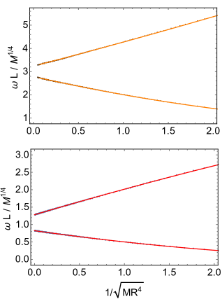
Figure 7: Lowest (bottom panel) and next-to-lowest (top panel) quasinormal frequencies for the scalar perturbation $\phi$. The solid (red and orange) lines are the fit.

We have solved the equation of motion for $\phi$ numerically, interpolating between a series solution at the boundary and a series solution at the horizon. Scanning through the complex frequency plane $\mathfrak{w}$, we have found the quasinormal frequencies as function of $x$, i.e we have found the curve $\mathfrak{w}=\mathfrak{w}(x)$. It is interesting to recover from this result the relation between $\omega$ and the scales of the problem, $M$ and $R$, according to dimensional analysis arguments. In fact, it is simple to show that in the limit of large $R$ there is only one possibility, $\mathfrak{w}(x)=c_{0}x^{1/4}$, and therefore $\omega L=c_{0}M^{1/4}$. The finite $R$ dependence instead is non trivial, and follows from the actual numerical solutions. The result fit into the ansatz,

$$\omega L=M^{1/4}\left(c_{0}+\frac{c_{1}}{x^{1/2}}+\frac{c_{2}}{x}+\ldots\right)\,,$$ (130)

where $\omega L$ is the proper frequency at the boundary. The numerical results for the lowest and the next-to-lowest quasi-normal modes are shown in Figure 7. For the lowest quasi-normal mode, the values of the first two coefficients in the fit ansatz (130) are,

$$c_{0} =\ 1.282-i\,0.824\,,$$

$$c_{1} =\ 0.763+i\,0.362\,,$$

$$c_{2} =-0.029-i\,0.041\,,$$ (131)

and for next-to-lowest quasi-normal mode,

$$c_{0} =\ 3.241-i\,2.786\,,$$

$$c_{1} =\ 0.985+i\,0.873\,,$$

$$c_{2} =\ 0.045-i0.093\leavevmode\nobreak\ .$$ (132)

VII VI.  Discussion

Connecting the dots of what we have done so far, we have two parallel situations in $\mathcal{N}=4$ SYM, a statistical ensemble on one side, a black hole on the other side, and two dynamical quantities which we can now compare: their lowest quasinormal frequency. Let us here emphasize that there is a-priori no reason why we should expect some kind of resemblance, but according to our findings, their qualitative behavior is surprisingly similar. The parameters, $\mathfrak{h}$ and $\mathfrak{m}$ in the BMN matrix model, and $M$ and $R$ in the black hole, determine the frequencies very much in the same way. In particular, it is an independent outcome of the two calculations that the leading correction to the flat or zero mass limit, written as an expansion in powers of $\mathfrak{m}^{4}/\mathfrak{h}$ and $1/MR^{4}$, is fixed by the power $p=1/2$. This result cannot be obtained by dimensional analysis. In the absence of a better analytical understanding, we can only appreciate the unexpected beauty of the precision fit in Figure 6 while considering its striking similarity with that of Figure 7.

Following the work of Berkowitz:2016jlq ; Catterall:2014vka , it would be interesting to compute semiclassical corrections to our Dyson fluid distribution, and see how the quasi-normal frequencies are modified at small but finite ’t Hooft coupling.

VIII VII.  Conclusions and Outlook

In this paper we have analyzed Dyson fluid solutions of the BMN matrix model living on Lagrangian sub-manifolds of the phase space. We have characterized the corresponding ensemble by symmetries, conserved charges, and at the equilibrium, by the expectation values of local operators. We have defined a novel gauge-invariant quench protocol which allowed us to deform the equilibrium distribution in a controlled way, and we have shown that the expectation values of twist two scalar operators in the $SO(6)$ sector re-equilibrate via quasi-normal oscillations. Finally, we have determined the numerical dependence of the complex frequency $\omega$ of the lowest quasi-normal mode as function of the energy $\mathfrak{h}$ and the dimensionless parameter $\mathfrak{m}^{4}/\mathfrak{h}$.

The interesting features of the Dyson-fluid are triggered by the non-commutative nature of the microscopic dynamics. The study of eigenvalue distributions of observables offers an alternative geometric picture of the dynamics. In particular, the complexity of an observable provides the tool to detect different type of correlations in the ensemble. In the second part of the paper we have compared the emergent geometric structure of our classical Dyson-fluid and the holographic geometry of a black hole at strong ’t Hooft coupling. Our main result has been to point out an unexpected similarity between the parametric behavior of the quasi-normal frequencies in the Dyson-fluid and in the black hole background.

There are similarities between the phase space picture of the quasi-normal oscillations, and the entropic principle of Verlinde:2010hp : A rigorous way to understand the process of equilibration would be to consider a covering of the allowed phase space and verify that the population in each patch does not change in time. In this language, we are then led to conjecture the existence of an effective actions whose equations of motions determine the equilibrium distributions of the operators. As it happens for the case of the Brownian motion Blaizot:2009ex , it would be interesting to rewrite the time evolution of the distributions in terms of fluid-like equations.

Acknowledgments.

We are in debt with: Diego Hofman, for valuable discussions and important comments on the draft at different stages of this work, Dario Villamaina, for collaboration at an early stage, and Vasilis Niarchos for important feedback on the final version of the draft. We would like to thank Nick Evans, for stimulating conversations which gave the start to the present work. We also thank M.Caldarelli, M.Hanada, G. Hartnett, K. Skenderis for discussions. Finally, we would like to thank an anonymous referee for pointing out several improvements in our narration. We acknowledge the use of the IRIDIS High Performance Computing Facility, and its associated support services at the University of Southampton. FA acknowledges support from STFC through Consolidated Grant ST/L000296/1. FS received funding from the European Research Council under the European Community Seventh Framework Programme (FP7/2007-2013) ERC grant agreement No 279757.

IX Appendix

IX.1 A.  Determination of the quasi-normal frequencies

For completeness, we describe in detail the algorithm we used to determine, at fixed $h$ and $\overline{\epsilon}$, the values of the parameters entering the ansatz

$${\cal O}(t)={\cal O}_{\infty}+e^{-t/\tau}\Big{(}d+u\cos(\omega t+\phi)\Big{)}\leavevmode\nobreak\ ,$$ (133)

of the lowest quasi-normal mode. The parameters are obtained by minimizing the $\chi^{2}$:

$$\chi^{2}=\sum_{t=t_{min}}^{t_{max}}\frac{{\cal O}(t)-\langle{\cal O}\rangle(t)}{\sigma^{2}(t)}\leavevmode\nobreak\ .$$ (134)

where $\langle{\cal O}\rangle(t)$ is defined in (42), and $\sigma(t)$ is the error on $\langle{\cal O}\rangle(t)$ estimated via jackknife analysis.

Setting the quench time at $t=0$ for convenience, the time $t_{\max}$ is chosen where the $\langle{\cal O}\rangle$ has equilibrated. In practise, we fix it to the time after which the physical oscillations of $\langle{\cal O}\rangle(t)$ are indistinguishable from the statistical fluctuations. In this way we minimize the contribution of irrelevant noise entering the $\chi^{2}$ at late times. Moreover, in order to isolate the lowest quasi-normal mode we have to choose a $t_{min}$ large enough such that the contributions to ${\cal O}(t)$ coming from faster decaying (higher) quasi-normal modes are negligible. This is determined by increasing $t_{min}$ progressively, from zero towards $t_{max}$, until the estimated frequencies are stable against a further variations of $t_{min}$. After subtracting the lowest quasi-normal mode from the signal, we could in principle repeat the procedure to isolate the next quasi-normal mode, and so on. A more sophisticated approach would be actually needed to improve the stability of the results. For simplicity, in this work we have focused mainly on the lowest one.

The errors on the frequencies are estimated from the spread of distribution of the fit parameters obtained from the different jacknife samples used.

IX.2 B.  On Quenches far-from-equilibrium

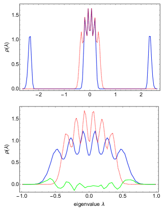
Figure 8: The distributions $\rho^{eig}_{\mathfrak{p}=4}$ for $N=6$ at different instants of time, $h=0.3$. Top panel: the dotted red curve corresponds to $t^{-}_{quench}$ and the solid blue curve to $t^{+}_{quench}$, with $\epsilon=2$. Bottom panel: the solid curves correspond to the $\rho^{eig}_{4}$ (blue) and $\rho^{eig}_{4}-\rho^{eig}_{5}$ (green) at the new equilibrium in ${\cal E}^{\prime}$, the dotted red curve is taken from the top panel.

In this section, we briefly describe edge-type quenches, in which $\mathcal{E}^{\prime}$ is a far-from-equilibrium configuration compared to $\mathcal{E}$. We also use these type of quenches to illustrate basic consequences of the explicit symmetry breaking which persists in the ensemble at the new equilibrium.

By construction, far-from-equilibrium configurations can be easily engineered by increasing the strength of the quench parameters. Considering a large value of the quench parameter $\epsilon$, the distribution of eigenvalues of $\rho^{eig}_{\mathfrak{p}}$ at $t^{+}_{quench}$ can be deformed as follows: $\rho^{eig}_{\mathfrak{p}}$ will contain three disconnected pieces, two outer peaks, whose support is very well separated, and a central “bubble” of eigenvalues. In the top panel of Figure 8 we show a snapshot of the distribution $\rho^{eig}_{\mathfrak{p}}$ at $t^{-}_{quench}$ and $t^{+}_{quench}$ for $N=6$ in the case of $\epsilon=2$ and $h=0.3$. It is worth emphasizing that this particular profile of $\rho^{eig}_{\mathfrak{p}}$ provides a different realization of the framework of Aoki:2015uha .

The time evolution of the distribution after the quench proceeds as the intuition suggests: The two outer peaks start moving towards the central region until a new equilibrium is reached. At the new equilibrium $\rho^{eig}_{\mathfrak{p}}$ has a unique support. The apparent attractive force between the outer and the central part of the density of eigenvalues should not be interpreted as originating from an attractive force in the microscopic potential. In fact, the flow is expansive. Instead, the nature of the force is statistical, and it appears in the chaotic regime as a consequence of the phase space getting populated according to the equilibrium distribution.

We can explore the symmetry breaking pattern after the quench by analysing the equilibrium distributions of $\rho^{eig}_{\mathfrak{p}}$ and $\rho^{eig}_{I\neq\mathfrak{p}}$, as shown in the bottom panel of Figure 8. The green histogram is the difference between $\rho^{eig}_{\mathfrak{p}}$ and $\rho^{eig}_{\i\neq\mathfrak{p}}$, and it is non vanishing. The symmetry breaking in the case of close-to-equilibrium quenches has less prominent features, but can be seen more clearly upon increasing the volume of the statistics. Finally, since the change in the conserved charges is non perturbative the expectation values of the charged operators $\mathcal{N}_{i=1,2}$ do not show a simple quasi-normal oscillation. Instead, they display a more complicated behavior in which the under and over-damping behaviors are equally mixed. A more sophisticated analysis than the one used in Appendix A would be needed to decompose the signal into a sum of quasi-normal modes.

References

- (1)
- (2) F. J. Dyson, J. Math. Phys. 3, 1191, (1962).
- (3) J. P. Blaizot and M. A. Nowak, Phys. Rev. E 82, 051115, (2010)
- (4) D. E. Berenstein, J. M. Maldacena and H. S. Nastase, JHEP 0204, 013 (2002) doi:10.1088/1126-6708/2002/04/013 [hep-th/0202021].
- (5) N. Kim, T. Klose and J. Plefka, Nucl. Phys. B 671, 359 (2003) doi:10.1016/j.nuclphysb.2003.08.019 [hep-th/0306054].
- (6) G. Gur-Ari, M. Hanada and S. H. Shenker, JHEP 1602, 091 (2016) doi:10.1007/JHEP02(2016)091 [arXiv:1512.00019 [hep-th]].
- (7) C. Asplund, D. Berenstein and D. Trancanelli, Phys. Rev. Lett. 107, 171602 (2011) doi:10.1103/PhysRevLett.107.171602 [arXiv:1104.5469 [hep-th]].
- (8) C. T. Asplund, D. Berenstein and E. Dzienkowski, Phys. Rev. D 87, no. 8, 084044 (2013) doi:10.1103/PhysRevD.87.084044 [arXiv:1211.3425 [hep-th]].
- (9) R. Gopakumar and D. J. Gross, Nucl. Phys. B 451, 379 (1995) doi:10.1016/0550-3213(95)00340-X [hep-th/9411021].
- (10) J. Gomis, S. Matsuura, T. Okuda and D. Trancanelli, JHEP 0808, 068 (2008) doi:10.1088/1126-6708/2008/08/068 [arXiv:0807.3330 [hep-th]].
- (11) A. Buchel, J. G. Russo and K. Zarembo, JHEP 1303, 062 (2013) doi:10.1007/JHEP03(2013)062 [arXiv:1301.1597 [hep-th]].
- (12) F. Benini, K. Hristov and A. Zaffaroni, JHEP 1605, 054 (2016) doi:10.1007/JHEP05(2016)054 [arXiv:1511.04085 [hep-th]].
- (13) H. Bantilan, F. Pretorius and S. S. Gubser, Phys. Rev. D 85, 084038 (2012) doi:10.1103/PhysRevD.85.084038 [arXiv:1201.2132 [hep-th]].
- (14) M. S. Costa, L. Greenspan, J. Penedones and J. Santos, JHEP 1503, 069 (2015) doi:10.1007/JHEP03(2015)069 [arXiv:1411.5541 [hep-th]].
- (15) T. Banks, W. Fischler, S. H. Shenker and L. Susskind, Phys. Rev. D 55, 5112 (1997) doi:10.1103/PhysRevD.55.5112 [hep-th/9610043].
- (16) I. P. Omelyan, I. M. Mryglod, and R. Folk, Phys. Rev. E 65, 056706 (2002) doi:10.1103/PhysRevE.65.056706 [arXiv:cond-mat/0110438].
- (17) Rainer Klages, “Introduction to Dynamical Systems,” School of Mathematical Sciences Queen Mary, University of London.
- (18) K. Ho, J.M. Kahn, Journal of Lightwave Technology, vol. 29, pp. 3119-3128, 2011 [arXiv:1104.4527v2 [physics.optics]]
- (19) S. Aoki, M. Hanada and N. Iizuka, JHEP 1507, 029 (2015) doi:10.1007/JHEP07(2015)029 [arXiv:1503.05562 [hep-th]].
- (20) J. M. Maldacena, Int. J. Theor. Phys. 38, 1113 (1999) [Adv. Theor. Math. Phys. 2, 231 (1998)] doi:10.1023/A:1026654312961 [hep-th/9711200].
- (21) E. D’Hoker and D. Z. Freedman, hep-th/0201253.
- (22) E. Witten, Adv. Theor. Math. Phys. 2, 253 (1998) [hep-th/9802150].
- (23) J. D. Bekenstein, Phys. Rev. D 7, 2333 (1973). doi:10.1103/PhysRevD.7.2333
- (24) G. W. Gibbons and S. W. Hawking, Phys. Rev. D 15, 2752 (1977). doi:10.1103/PhysRevD.15.2752
- (25) For a quick comparison with the notation of Maldacena:1997re , our is such that .
- (26) E. Berti, V. Cardoso and A. O. Starinets, Class. Quant. Grav. 26, 163001 (2009) doi:10.1088/0264-9381/26/16/163001 [arXiv:0905.2975 [gr-qc]].
- (27) J. T. Liu and W. A. Sabra, Phys. Rev. D 72, 064021 (2005) doi:10.1103/PhysRevD.72.064021 [hep-th/0405171].
- (28) E. Witten, Adv. Theor. Math. Phys. 2, 505 (1998) [hep-th/9803131].
- (29) M. Cvetic, H. Lu, C. N. Pope, A. Sadrzadeh and T. A. Tran, Nucl. Phys. B 586, 275 (2000) doi:10.1016/S0550-3213(00)00372-2 [hep-th/0003103].
- (30) K. Skenderis and M. Taylor, JHEP 0608, 001 (2006) doi:10.1088/1126-6708/2006/08/001 [hep-th/0604169].
- (31) M. Bianchi, D. Z. Freedman and K. Skenderis, Nucl. Phys. B 631, 159 (2002) doi:10.1016/S0550-3213(02)00179-7 [hep-th/0112119].
- (32) G. T. Horowitz and V. E. Hubeny, Phys. Rev. D 62, 024027 (2000) doi:10.1103/PhysRevD.62.024027 [hep-th/9909056].
- (33) E. Berti, V. Cardoso and J. P. S. Lemos, Phys. Rev. D 70, 124006 (2004) doi:10.1103/PhysRevD.70.124006 [gr-qc/0408099].
- (34) G. T. Horowitz and J. Polchinski, Phys. Rev. D 55, 6189 (1997) doi:10.1103/PhysRevD.55.6189 [hep-th/9612146].
- (35) E. Berkowitz, E. Rinaldi, M. Hanada, G. Ishiki, S. Shimasaki and P. Vranas, arXiv:1606.04951 [hep-lat].
- (36) S. Catterall, D. Schaich, P. H. Damgaard, T. DeGrand and J. Giedt, Phys. Rev. D 90, no. 6, 065013 (2014) doi:10.1103/PhysRevD.90.065013 [arXiv:1405.0644 [hep-lat]].
- (37) E. P. Verlinde, JHEP 1104, 029 (2011) doi:10.1007/JHEP04(2011)029 [arXiv:1001.0785 [hep-th]].