The space density of luminous dusty star-forming galaxies at $z>4$:
SCUBA-2 and LABOCA imaging of ultrared galaxies from Herschel-ATLAS

Abstract

Until recently, only a handful of dusty, star-forming galaxies (DSFGs) were known at $z>4$, most of them significantly amplified by gravitational lensing. Here, we have increased the number of such DSFGs substantially, selecting galaxies from the uniquely wide 250-, 350- and 500-$\mu$m Herschel-ATLAS imaging survey on the basis of their extremely red far-infrared colors and faint 350- and 500-$\mu$m flux densities – ergo they are expected to be largely unlensed, luminous, rare and very distant. The addition of ground-based continuum photometry at longer wavelengths from the James Clerk Maxwell Telescope (JCMT) and the Atacama Pathfinder Experiment (APEX) allows us to identify the dust peak in their spectral energy distributions (SEDs), better constraining their redshifts. We select the SED templates best able to determine photometric redshifts using a sample of 69 high-redshift, lensed DSFGs, then perform checks to assess the impact of the CMB on our technique, and to quantify the systematic uncertainty associated with our photometric redshifts, $\sigma=0.14\,(1+z)$, using a sample of 25 galaxies with spectroscopic redshifts, each consistent with our color selection. For Herschel-selected ultrared galaxies with typical colors of $S_{500}/S_{250}\sim 2.2$ and $S_{500}/S_{350}\sim 1.3$ and flux densities, $S_{500}\sim 50$ mJy, we determine a median redshift, $\hat{z}_{\rm phot}=3.66$, an interquartile redshift range, 3.30–4.27, with a median rest-frame 8–1000-$\mu$m luminosity, $\hat{L}_{\rm IR}$, of $1.3\times 10^{13}$ L_⊙. A third lie at $z>4$, suggesting a space density, $\rho_{z>4}$, of $\approx 6\times 10^{-7}$ Mpc^-3. Our sample contains the most luminous known star-forming galaxies, and the most over-dense cluster of starbursting proto-ellipticals yet found.

1. Introduction

The first deep submillimeter (submm) imaging surveys – made possible by large, ground-based telescopes equipped with highly multiplexed bolometer arrays (e.g. Kreysa et al., 1998; Holland et al., 1999) – resolved a previously unknown population of submm-bright galaxies, or dusty star-forming galaxies (hereafter DSFGs — Smail et al., 1997; Barger et al., 1998; Hughes et al., 1998). Interferometric imaging refined the positions of these DSFGs sufficiently to allow conventional optical spectroscopic observations, and they were then shown to lie at $z>1$ (e.g. Chapman et al., 2003), and to be a thousand times more numerous than their supposed local analogs, ultraluminous infrared (IR) galaxies (ULIRGs — e.g. Sanders & Mirabel, 1996).

The Spectral and Photometric Imaging Receiver (SPIRE — Griffin et al., 2010) on board Herschel (Pilbratt et al., 2010) gave astronomers a new tool to select dusty galaxies. Moreover, simultaneous imaging through three far-infrared filters at 250, 350 and 500 $\mu$m enables the selection of ‘ultrared DSFGs’ in the early Universe, $z>4$. The space density and physical properties of the highest-redshift starbursts provide some of the most stringent constraints on galaxy-formation models, since these galaxies lie on the most extreme tail of the galaxy stellar mass function (e.g. Hainline et al., 2011).

Cox et al. (2011) were the first to search amongst the so-called ‘500-$\mu$m risers’ ($S_{250}<S_{350}<S_{500}$, where $S_{\lambda}$ is the flux density at $\lambda$ $\mu$m), reporting extensive follow-up observations of one of the brightest, reddest DSFGs in the first few 16-deg² tiles of the $\approx 600$-deg² imaging survey, H-ATLAS (Herschel Astrophysical Terahertz Large Area Survey — Eales et al., 2010), a lensed starburst at $z=4.2$, G15.141 or HATLAS J142413.9$+$022304, whose clear, asymmetric double-peaked CO lines betray an asymmetric disk or ring, and/or the near-ubiquitous merger found in such systems (Engel et al., 2010). Dowell et al. (2014) demonstrated the effectiveness of a similar SPIRE color-selection technique, finding 1HERMES S350 J170647.8$+$584623 at $z=6.3$ (Riechers et al., 2013) in the northern 7-deg² First Look Survey field (see also Asboth et al., 2016). Meanwhile, relatively wide and shallow surveys with the South Pole Telescope (SPT) have allowed the selection of large numbers of gravitationally lensed DSFGs (Vieira et al., 2010). These tend to contain cold dust and/or to lie at high redshifts (Vieira et al., 2013; Weiß et al., 2013; Strandet et al., 2016), due in part to their selection at wavelengths beyond 1 mm, which makes the survey less sensitive to warmer sources at $z\approx 1$–3.

In this paper, we report efforts to substantially increase the number of ultrared DSFGs, using a similar color-selection method to isolate colder and/or most distant galaxies, at $z>4$, a redshift regime where samples are currently dominated by galaxies selected in the rest-frame ultraviolet (e.g. Ellis et al., 2013). Our goal here is to select galaxies that are largely unlensed, rare and very distant, modulo the growing optical depth to lensing at increasing redshift. We hope to find the progenitors of the most distant quasars, of which more than a dozen are known to host massive ($>10^{8}$ M_⊙) black holes at $z>6$ (e.g. Fan et al., 2001; Mortlock et al., 2011). We would expect to find several in an area the size of H-ATLAS, $\approx 600$ deg², if the duration of their starburst phase is commensurate with their time spent as ‘naked’ quasars. We accomplish this by searching over the whole H-ATLAS survey area – an order of magnitude more area than the earlier work in H-ATLAS.

We exploit both ground- and space-based observations, concentrating our efforts in a flux-density regime, $S_{\rm 500}<100$ mJy where most DSFGs are not expected to be boosted significantly by gravitational lensing (Negrello et al., 2010; Conley et al., 2011). We do this partly to avoid the uncertainties associated with lensing magnification corrections and differential magnification (e.g. Serjeant, 2012), partly because the areal coverage of our Herschel survey would otherwise yield only a handful of targets, and partly because wider surveys with the SPT are better suited to finding the brighter, distant, lensed population.

In the next section we describe our data acquisition and our methods of data reduction. We subsequently outline our sample selection criteria before presenting, analyzing, interpreting and discussing our findings in §4. Our conclusions are outlined in §5. Follow-up spectral scans of a subset of these galaxies with the Atacama Large Millimeter Array (ALMA) and with Institute Radioastronomie Millimetrique’s (IRAM’s) Northern Extended Millimeter Array (NOEMA) are presented by Fudamoto et al. (2016). Following the detailed ALMA study by Oteo et al. (2016d) of one extraordinarily luminous DSFG from this sample, Oteo et al. (2016b) present high-resolution continuum imaging of a substantial subset of our galaxies, determining the size of their star-forming regions and assessing the fraction affected by gravitational lensing. Submillimeter imaging of the environments of the reddest galaxies using the 12-m Atacama Pathfinder Telescope (APEX) are presented by Lewis et al. (2016). A detailed study of a cluster of starbursting proto-ellipticals centered on one of our reddest DSFGs is presented by Oteo et al. (2016c).

We adopt a cosmology with $H_{0}=71$ km s^-1 Mpc^-1, $\Omega_{\rm m}=0.27$ and $\Omega_{\Lambda}=0.73$.

2. Sample selection

2.1. Far-infrared imaging

We utilize images created for the H-ATLAS Data Release 1 (Valiante et al., 2016), covering three equatorial fields with right ascensions of 9, 12 and 15 hr, the so-called GAMA09, GAMA12 and GAMA15 fields, each covering $\approx 54$ deg²; in the north, we also have $\approx 170$ deg² of areal coverage in the North Galactic Pole (NGP) field; finally, in the south, we have $\approx 285$ deg² in the South Galactic Pole (SGP) field, making a total of $\approx 600$ deg². The acquisition and reduction of these Herschel parallel-mode data from SPIRE and PACS (Photoconductor Array Camera and Spectrometer — Poglitsch et al., 2010) for H-ATLAS are described in detail by Valiante et al. (2016). Summarising quickly: before the subtraction of a smooth background or the application of a matched filter, as described next in §2.2, the 250-, 350- and 500-$\mu$m SPIRE maps exploited here have 6, 8 and 12^′′ pixels, point spread functions (PSFs) with azimuthally-averaged fwhm of 17.8, 24.0 and 35.2^′′ and mean instrumental [confusion] r.m.s. noise levels of 9.4 [7.0], 9.2 [7.5] and 10.6 [7.2] mJy, respectively, where $\sigma_{\rm total}=\sqrt{\sigma^{2}_{\rm conf}+\sigma^{2}_{\rm instr}}$.

2.2. Source detection

Sources were identified and flux densities were measured using a modified version of the Multi-band Algorithm for source eXtraction (madx; Maddox et al., in prep). madx first subtracted a smooth background from the SPIRE maps, and then filtered them with a ‘matched filter’ appropriate for each band, designed to mitigate the effects of confusion (e.g. Chapin et al., 2011). At this stage, the map pixel distributions in each band have a highly non-Gaussian positive tail because of the sources in the maps, as discussed at length for the unfiltered maps by Valiante et al. (2016).

Next, 2.2-$\sigma$ peaks were identified in the 250-$\mu$m map, and ‘first-pass’ flux-density estimates were obtained from the pixel values at these positions in each SPIRE band. Sub-pixel positions were estimated by fitting to the 250-$\mu$m peaks, then more accurate flux densities were estimated using bi-cubic interpolation to these improved positions. In each band, the sources were sorted in order of decreasing flux density using the first-pass pixel values, and a scaled PSF was subtracted from the map, leaving a residual map used to estimate fluxes for any fainter sources. This step prevents the flux densities of faint sources being overestimated when they lie near brighter sources. In the modified version of madx, the PSF subtraction was applied only for sources with 250-$\mu$m peaks greater than 3.2$\sigma$. The resulting 250-$\mu$m-selected sources were labelled as bandflag=1 and the pixel distribution in the residual 250-$\mu$m map is now close to Gaussian, since all of the bright 250-$\mu$m sources have been subtracted.

The residual 350-$\mu$m map, in which the pixel distribution retains a significant non-Gaussian positive excess, was then searched for sources, using the same algorithms as for the initial 250-$\mu$m selection. Sources with peak significance more than 2.4-$\sigma$ in the 350-$\mu$m residual map are saved as bandflag=2 sources. Next, the residual 500-$\mu$m map was searched for sources, and 2.0-$\sigma$ peaks are saved as bandflag=3 sources.

Although the pixel distributions in the final 350- and 500-$\mu$m residual images are much closer to Gaussian than the originals, a significant non-Gaussian positive tail remains, due to subtracting PSFs from sources that are not well fit by the PSF. Some of these are multiple sources detected as a single blend, while some are extended sources. Since even a single, bright, extended source can leave hundreds of pixels with large residuals — comparable to the residuals from multiple faint red sources — it is not currently feasible to disentangle the two.

For the final catalogue, we keep sources only if they are above 3.5$\sigma$ in any one of the three SPIRE bands. For each source, the astrometric position was determined by the data in the initial detection band. No correction for flux boosting has been applied. The catalogue thus created contains $7\times 10^{5}$ sources across the five fields observed as part of H-ATLAS.

2.3. Parent sample of ultrared DSFG candidates

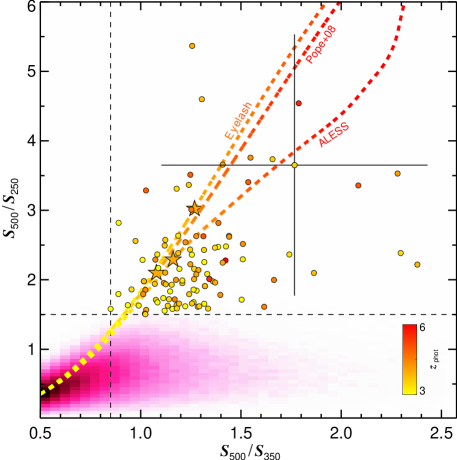
Figure 1.— $S_{350}/S_{500}$ versus $S_{250}/S_{500}$ for our sample, overlaid with the redshift tracks expected for a galaxy with the SED of the Cosmic Eyelash (Swinbank et al., 2010; Ivison et al., 2010) and for two SED templates that were synthesized for submm-selected DSFGs by Pope et al. (2008) and Swinbank et al. (2014, ALESS). To match our color-selection criteria, galaxies must have $S_{500}/S_{250}\geq 1.5$ and $S_{500}/S_{350}\geq 0.85$ and thus lie in the top-right region of the plot. The points representing our sample (and the redshift track) are color-coded according to their photometric redshifts, as described in §4.2. The $z=4$ points on the redshift tracks are marked with orange stars. A representative color uncertainty is shown. Sources from the Phase 1 data release of H-ATLAS lie in the black-pink cloud (Valiante et al., 2016).

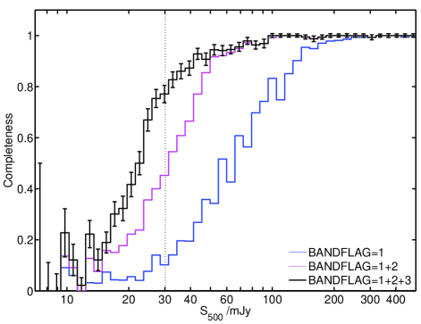
Figure 2.— Completeness as a function of 500-$\mu$m flux density, as assessed by injecting fake sources with colors consistent with the SEDs of the ultrared DSFGs we expect to detect. For the individual fake SPIRE images (see §2.3.1), completeness is consistent with expectations for sources at a given signal-to-noise ratio (SNR). Using all three bandflag values results in a relatively high level of completeness ($77\pm 3$%) down to 30 mJy, the flux-density level (marked with a dotted line) at which we have selected our sample. Adding the bandflag=2 and 3 sources improves the completeness significantly.

Definition of our target sample began with the 7,961 sources detected at $\geq 3.5$-$\sigma$ at 500 $\mu$m, with $S_{500}/S_{250}\geq 1.5$ and $S_{500}/S_{350}\geq 0.85$, as expected for DSFGs at $z\mathrel{\raise 1.50696pt\hbox{$\scriptstyle>$}\kern-6.00006pt\lower 1.72218pt\hbox{{$\scriptstyle\sim$}}}4$ (see the redshift tracks of typical DSFGs, e.g. the Cosmic Eyelash, SMM J2135$-$0102 — Swinbank et al., 2010; Ivison et al., 2010, in Fig. 1) of which 29, 42 and 29% are bandflag = 1, 2 and 3, respectively.

2.3.1 Conventional completeness

To calculate the fraction of real, ultrared DSFGs excluded from the parent sample because of our source detection procedures, we injected 15,000 fake, PSF-convolved point sources into our H-ATLAS images (following Valiante et al., 2016) with colors corresponding to the spectral energy distribution (SED) of a typical DSFG, the Cosmic Eyelash, at redshifts between 0 and 10. The mean colors of these fake sources were $S_{500}/S_{250}=2.25$ and $S_{500}/S_{350}=1.16$, cf. the median colors for the sample chosen for ground-based imaging (§2.3.2), $S_{500}/S_{250}=2.15$ and $S_{500}/S_{350}=1.26$, so similar. Values of $S_{250}$ were set to give a uniform distribution in log${}_{10}\,S_{250}$. We then re-ran the same source detection process described above (§2.2), as for the real data, matching the resulting catalog to the input fake catalog.

To determine the completeness for the ultrared sources, we have examined how many of the recovered fake sources match our color criteria, as a function of input $S_{500}$ and bandflag. Fig. 2 shows how adding the bandflag=2 and 3 sources improves the completeness: the blue line is for bandflag=1 only; magenta is for bandflag=1 and 2, and black shows bandflag=1, 2 and 3. Selecting only at 250 $\mu$m yields a completeness of 80% at 100 mJy; including bandflag=2 sources pushes us down to 50 mJy; using all three bandflag values gets us down to 30 mJy. We estimate a completeness at the flux-density and color limits of the sample presented here of $77\pm 3$%.

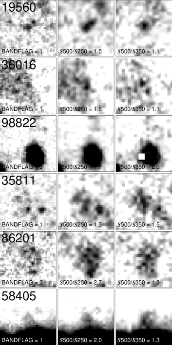
Figure 3.— Herschel SPIRE imaging of candidate ultrared DSFGs from our parent sample of 7,961 sources, each displayed from $-6$ to +60 mJy beam^-1, chosen to illustrate the different reasons that sources were excluded from the sample to be observed by SCUBA-2 and LABOCA by our eyeballing team. In each column, from left to right, we show 250-, 350- and 500-$\mu$m cut-out images, each $3^{\prime}\times 3^{\prime}$ and centered on the (labelled) galaxy. The 250-$\mu$m cut-out images have been convolved with a 7^′′ Gaussian. North is up and East is left. The field labelled 19560 is an example where emission from one or more 250-$\mu$m sources is missed or dealt with poorly by madx, leading to misleading colors. None of the candidates in this category are likely to be genuine, ultrared DSFGs. The examples labelled 36016, 35811 and 86201 show confused regions in which the madx flux densities and colors were judged unreliable. We estimate that up to $\approx$55% of these fields could contain genuine, ultrared DSFGs. The bright galaxy in the field labelled 98822 has led to a spurious detection by madx – such examples are rare, fortunately, and madx is in fact capable of identifying plausible ultrared DSFGs alongside very bright, local galaxies, as illustrated in the lower row for the field labelled 58405.

2.3.2 Eyeballing

Of these sources, a subset of 2,725 were eyeballed by a team of five (RJI, AJRL, VA, AO, HD) to find a reliable sub-sample for imaging with SCUBA-2 and LABOCA. As a result of this step, 708 ($26\pm 5$%) of the eyeballed sources were deemed suitable for ground-based follow-up observations, where the uncertainty is taken to be the scatter amongst the fractions determined by individual members of the eyeballing team. Fig. 3 shows typical examples of the remainder – those not chosen – usually because visual inspection revealed that blue (250-$\mu$m) emission had been missed or underestimated by madx (49% of cases). None of these are likely to be genuine, ultrared DSFGs. The next most common reason for rejection (22% of cases) was heavy confusion, such that the assigned flux densities and colors were judged to be unreliable. For the remaining 3%, the 350- and/or 500-$\mu$m morphologies were suggestive of Galactic cirrus or an imaging artifact.

2.3.3 Completeness issues related to eyeballing

Our team of eyeballers estimated that up to 14% of the candidates excluded by our eyeballing team – i.e. up to 55% of those in the latter two categories discussed in §2.3.2, or plausibly roughly half as many again as those deemed suitable for ground-based follow-up observations – could in fact be genuine, ultrared DSFGs. Phrased another way, the procedure was judged to recover at least 64% of the genuine, ultrared DSFGs in the parent sample.

Without observing a significant subset of the parent sample with SCUBA-2 or LABOCA, which would be prohibitively costly and inefficient, it is not possible to know exactly what fraction of genuine, ultrared DSFGs were missed because of our eyeballing procedure. However, it is possible to determine the fraction of sources that were missed in a more quantitative manner than we have accomplished thus far. To do this, a sample of 500 fake, injected ultrared sources – with the same flux density and color distribution as the initial sample – were given to the same team of eyeballers for classification, using the same criteria they had used previously, along with the same number of real, ultrared DSFG candidates. The fraction of genuine, ultrared DSFGs accepted by the eyeballing team is then taken to be the fraction of fake, injected sources assessed to be worthy of follow-up observations during this eyeballing process: $69\pm 8$%, cf. at least 64%, as estimated earlier by the eyeballing team.

2.4. Summary of issues affecting sample completeness

Since we have faced a considerable number of completeness issues, it is worth summarising their influence on our sample.

Based on robust simulations, we estimate that $\mathcal{C_{\rm MADX}}=77\pm 3$% of genuine, ultrared DSFGs made it through our madx cataloging procedures; of these, we eyeballed $\mathcal{C_{\rm eye}}=34$%, of which $26\pm 5$% were deemed suitable for follow-up observations with SCUBA-2 and/or LABOCA by our eyeballing team. A final set of simulations suggest that the eyeballing process was able to recover $\mathcal{C_{\rm check}}=69\pm 8$% of the available ultrared DSFG population from the parent madx catalog.

Of those selected for further study, a random subset of 109 were observed with SCUBA-2 and/or LABOCA (§3), just over $\mathcal{C_{\rm obs}}=15$% of the sample available from our eyeballing team. Their SPIRE colors are shown in Fig. 1. The bandflag $=1$, 2 and 3 subsets make up 48, 53 and 8 of this final sample, respectively.

To estimate the number of $z>4$ DSFGs across our survey fields, detectable to $S_{500}>30$ mJy with $S_{500}/S_{250}\geq 1.5$ and $S_{500}/S_{350}\geq 0.85$, we must scale up the number of $z>4$ DSFGs found amongst these 109 targets by $\mathcal{C_{\rm MADX}}\times\mathcal{C_{\rm eye}}\times\mathcal{C_{\rm check}}\times\mathcal{C_{\rm obs}})^{-1}=36.0\pm 8.2$, where we have included (in quadrature) the uncertainty in the fraction deemed suitable for follow-up observations with SCUBA-2 and/or LABOCA. In a more conventional sense, the completeness, $\mathcal{C}=0.028\pm 0.006$.

We note that although we are unable to satisfactorily quantify the number of DSFGs scattered by noise from the cloud shown in the bottom-left corner of Fig. 1 into our ultrared DSFG color regime, these DSFGs will be amongst the fraction shown to lie at $z_{\rm phot}<4$ (§4.2) and so a further correction to the space density of $z>4$ DSFGs (§4.3) is not required.

3. Submm observations and data reduction

3.1. 850-$\mu$m continuum imaging with SCUBA-2

Observations of 109 ultrared DSFGs were obtained using SCUBA-2 (Holland et al., 2013), scheduled flexibly during the period 2012–13, in good or excellent weather. The precipitable water vapor (PWV) was in the range 0.6–2.0 mm, corresponding to zenith atmospheric opacities of $\approx 0.2$–0.4 in the SCUBA-2 filter centered at 850 $\mu$m with a passband width to half power of 85 $\mu$m. The fwhm of the main beam is 13.0^′′ at 850 $\mu$m, before smoothing, with around 25% of the total power in the much broader [49^′′] secondary component (see Holland et al., 2013).

The observations were undertaken whilst moving the telescope at a constant speed in a so-called daisy pattern (Holland et al., 2013), which provides uniform exposure-time coverage in the central 3^′-diameter region of a field, but useful coverage over 12^′.

Around 10–15 min was spent integrating on each target, typically (see Table 1), sufficient to detect 850-$\mu$m emission robustly for $z>4$ far-IR-bright galaxies with a characteristic temperature of 10–100 k.

The flux-density scale was set using Uranus and Mars, and also secondary calibrators from the JCMT calibrator list (Dempsey et al., 2013), with estimated calibration uncertainties amounting to 5% at 850 $\mu$m. Since we visited each target only once (the handful of exceptions are noted in Table 1), the astrometry of the SCUBA-2 images is expected to be the same as the JCMT r.m.s. pointing accuracy, 2–3 arcsec.

The data were reduced using the Dynamic Iterative Map-Maker within the starlink smurf package (Chapin et al., 2013) using the ‘zero-mask’ algorithm, wherein the image is assumed to be free of significant emission apart from one or more specified regions, in our case a 30-arcsec-diameter circle (larger where appropriate, e.g. for SGP-354388 – see §4.1) centered on the target. This method is effective at suppressing large-scale noise. SCUBA-2 observations of flux density calibrators are handled in a similar manner, generally, so measuring reliable flux densities is significantly more straightforward than in other situations, as discussed later in §4.

3.2. 870-$\mu$m continuum imaging with LABOCA

Images were also taken with the Large APEX bolometer camera (LABOCA — Siringo et al., 2009) mounted on the 12-m Atacama Pathfinder EXperiment (APEX) telescope, on Llano Chajnantor at an altitude of 5,100 m, in Chile. LABOCA contains an array of 295 composite bolometers, arranged as a central channel with nine concentric hexagons, operating at a central wavelength of 870 $\mu$m (806–958 $\mu$m at half power, so a wider and redder passband than the SCUBA-2 850-$\mu$m filter) with a fwhm resolution of 19.2^′′.

All sources were observed using a compact raster pattern in which the telescope performed a 2.5^′-diameter spiral at constant angular speed at each of four raster positions, leading to a fully sampled map over the full 11^′-diameter field of view of LABOCA. Around 2–4 hr was spent integrating on each target (see Table 1). The data were reduced using the BoA software package, applying standard reductions steps (see e.g. Weiß et al., 2009).

The PWV during the observations was typically between 0.6 and 1.4 mm, corresponding to a zenith atmospheric opacity of 0.30–0.55 in the LABOCA passband. The flux-density scale was determined to an accuracy of 10% using observations of Uranus and Neptune. Pointing was checked every hour using nearby quasars and was stable. The astrometry of our LABOCA images, each the result of typically three individual scans, separated by pointing checks, is expected to be $\sigma\approx 1$–2^′′.

Table 1Targets and their properties.

IAU name	Nickname	Band	$S_{250}$		$S_{350}$		$S_{500}$		$S_{850}^{\rm peak}$		$S_{850}^{\rm 45}$		$S_{850}^{\rm 60}$		Date
		flag	/mJy		/mJy		/mJy		/mJy		/mJy		/mJy		observeda
HATLAS 085612.1$-$004922	G09$-$47693	1	27.4 $\pm$	7.3	34.4 $\pm$	8.1	45.4 $\pm$	8.6	12.5 $\pm$	4.0	6.4 $\pm$	9.1	5.4 $\pm$	10.8	2012$-$04$-$28
HATLAS 091642.6$+$022147	G09$-$51190	1	28.5 $\pm$	7.6	39.5 $\pm$	8.1	46.6 $\pm$	8.6	15.2 $\pm$	3.8	28.3 $\pm$	7.3	24.2 $\pm$	8.7	2012$-$12$-$21
HATLAS 084113.6$-$004114	G09$-$59393	1	24.1 $\pm$	7.0	43.8 $\pm$	8.3	46.8 $\pm$	8.6	23.7 $\pm$	3.5	27.7 $\pm$	5.6	12.4 $\pm$	9.8	2012$-$04$-$27
HATLAS 090925.0$+$015542	G09$-$62610	1	18.6 $\pm$	5.4	37.3 $\pm$	7.4	44.3 $\pm$	7.8	19.5 $\pm$	4.9	23.1 $\pm$	9.0	32.7 $\pm$	14.4	2012$-$03$-$06
HATLAS 091130.1$-$003846	G09$-$64889	1	20.2 $\pm$	5.9	30.4 $\pm$	7.7	34.7 $\pm$	8.1	15.1 $\pm$	4.3	4.4 $\pm$	8.9	$-$21.2 $\pm$	10.0	2012$-$12$-$16
HATLAS 083909.9$+$022718	G09$-$79552	2	16.6 $\pm$	6.2	38.1 $\pm$	8.1	42.8 $\pm$	8.5	17.0 $\pm$	3.6	11.1 $\pm$	7.3	3.2 $\pm$	14.0	2013$-$03$-$09
HATLAS 090419.9$-$013742	G09$-$79553	2	14.0 $\pm$	5.9	36.8 $\pm$	8.0	35.9 $\pm$	8.4	16.8 $\pm$	3.7	20.1 $\pm$	7.1	14.4 $\pm$	10.1	2013$-$03$-$09
HATLAS 084659.0$-$004219	G09$-$80620	2	13.5 $\pm$	5.0	25.3 $\pm$	7.4	28.4 $\pm$	7.7	13.2 $\pm$	4.3	6.8 $\pm$	9.8	$-$9.7 $\pm$	9.3	2012$-$12$-$16
HATLAS 085156.0$+$020533	G09$-$80658	2	17.8 $\pm$	6.4	31.6 $\pm$	8.3	39.5 $\pm$	8.8	17.6 $\pm$	4.1	13.6 $\pm$	9.4	24.0 $\pm$	9.4	2013$-$03$-$09
HATLAS 084937.0$+$001455	G09$-$81106	2	14.0 $\pm$	6.0	30.9 $\pm$	8.2	47.5 $\pm$	8.8	30.2 $\pm$	5.2	37.4 $\pm$	11.4	37.0 $\pm$	12.0	2012$-$12$-$18
HATLAS 084059.3$-$000417	G09$-$81271	2	15.0 $\pm$	6.1	30.5 $\pm$	8.2	42.3 $\pm$	8.6	29.7 $\pm$	3.7	35.8 $\pm$	6.4	44.2 $\pm$	10.6	2013$-$03$-$09
HATLAS 090304.2$-$004614	G09$-$83017	2	10.2 $\pm$	5.7	26.4 $\pm$	8.0	37.2 $\pm$	8.8	16.1 $\pm$	4.4	17.9 $\pm$	9.4	1.7 $\pm$	9.1	2012$-$12$-$16
HATLAS 090045.4$+$004125	G09$-$83808	2	9.7 $\pm$	5.4	24.6 $\pm$	7.9	44.0 $\pm$	8.2	36.0 $\pm$	3.1	36.2 $\pm$	9.1	23.5 $\pm$	10.4	2012$-$12$-$16
HATLAS 083522.1$+$005228	G09$-$84477	2	20.0 $\pm$	6.6	27.3 $\pm$	8.3	31.6 $\pm$	9.0	7.6 $\pm$	3.8	$-$6.5 $\pm$	7.4	$-$25.8 $\pm$	8.9	2012$-$04$-$27
HATLAS 090916.2$+$002523	G09$-$87123	2	10.4 $\pm$	5.8	25.3 $\pm$	8.2	39.2 $\pm$	8.7	20.7 $\pm$	4.6	24.5 $\pm$	9.3	43.7 $\pm$	12.4	2012$-$12$-$16
HATLAS 090855.6$+$015638	G09$-$100369	2	15.4 $\pm$	5.5	17.3 $\pm$	7.6	32.3 $\pm$	8.0	13.2 $\pm$	3.6	22.1 $\pm$	8.2	14.3 $\pm$	9.8	2013$-$03$-$09
HATLAS 090808.9$+$015459	G09$-$101355	3	9.5 $\pm$	5.5	14.6 $\pm$	7.9	33.4 $\pm$	8.3	13.5 $\pm$	4.9	$-$2.5 $\pm$	10.0	$-$40.2 $\pm$	12.7	2012$-$12$-$16
HATLAS 115415.5$-$010255	G12$-$34009	1	30.2 $\pm$	7.2	36.3 $\pm$	8.2	60.4 $\pm$	8.7	39.9 $\pm$	4.2	38.9 $\pm$	9.0	38.2 $\pm$	17.5	2013$-$03$-$09
HATLAS 114314.6$+$002846	G12$-$42911	1	21.2 $\pm$	5.8	44.1 $\pm$	7.4	53.9 $\pm$	7.7	35.4 $\pm$	3.6	32.8 $\pm$	7.0	21.0 $\pm$	8.0	2012$-$04$-$27
HATLAS 114412.1$+$001812	G12$-$66356	1	18.3 $\pm$	5.4	26.5 $\pm$	7.4	32.9 $\pm$	7.8	11.2 $\pm$	4.6	$-$7.5 $\pm$	8.8	$-$2.2 $\pm$	12.5	2012$-$12$-$18
HATLAS 114353.5$+$001252	G12$-$77450	2	14.8 $\pm$	5.1	27.3 $\pm$	7.4	35.9 $\pm$	7.7	11.9 $\pm$	4.1	$-$0.3 $\pm$	7.9	$-$6.3 $\pm$	8.7	2012$-$04$-$27
HATLAS 115012.2$-$011252	G12$-$78339	2	17.0 $\pm$	6.2	30.8 $\pm$	8.1	31.6 $\pm$	9.0	18.1 $\pm$	4.3	31.3 $\pm$	8.9	33.3 $\pm$	11.2	2012$-$04$-$27
HATLAS 115614.2$+$013905	G12$-$78868	2	13.1 $\pm$	5.9	29.5 $\pm$	8.2	49.0 $\pm$	8.5	12.2 $\pm$	3.5	13.6 $\pm$	6.4	5.8 $\pm$	9.6	2012$-$04$-$27
HATLAS 114038.8$-$022811	G12$-$79192	2	15.8 $\pm$	6.3	28.6 $\pm$	8.1	34.1 $\pm$	8.8	5.1 $\pm$	3.5	$-$4.3 $\pm$	6.4	$-$17.4 $\pm$	7.8	2012$-$12$-$21
HATLAS 113348.0$-$002930	G12$-$79248	2	18.4 $\pm$	6.2	29.5 $\pm$	8.2	42.0 $\pm$	8.9	27.6 $\pm$	5.0	62.4 $\pm$	9.8	71.3 $\pm$	12.0	2012$-$12$-$18
HATLAS 114408.1$-$004312	G12$-$80302	2	15.9 $\pm$	6.2	27.2 $\pm$	8.1	35.9 $\pm$	9.0	6.0 $\pm$	3.8	$-$15.0 $\pm$	8.9	$-$28.8 $\pm$	9.5	2012$-$04$-$27
HATLAS 115552.7$-$021111	G12$-$81658	2	14.9 $\pm$	6.1	26.5 $\pm$	8.1	36.8 $\pm$	8.7	1.0 $\pm$	4.4	$-$25.5 $\pm$	8.7	$-$32.0 $\pm$	12.2	2012$-$12$-$21
HATLAS 113331.1$-$003415	G12$-$85249	2	13.3 $\pm$	6.1	25.0 $\pm$	8.3	31.4 $\pm$	8.8	4.4 $\pm$	2.7	$-$0.3 $\pm$	5.7	$-$3.3 $\pm$	6.6	2012$-$12$-$18
HATLAS 115241.5$-$011258	G12$-$87169	2	13.5 $\pm$	6.0	23.5 $\pm$	8.2	33.5 $\pm$	8.8	6.9 $\pm$	4.0	9.8 $\pm$	9.2	6.1 $\pm$	9.6	2012$-$12$-$21
HATLAS 114350.1$-$005211	G12$-$87695	2	19.0 $\pm$	6.4	23.9 $\pm$	8.3	30.7 $\pm$	8.7	15.6 $\pm$	3.9	2.2 $\pm$	7.1	$-$6.2 $\pm$	10.4	2012$-$12$-$21
HATLAS 142208.7$+$001419	G15$-$21998	1	36.0 $\pm$	7.2	56.2 $\pm$	8.1	62.6 $\pm$	8.8	13.2 $\pm$	3.4	7.2 $\pm$	7.0	7.3 $\pm$	9.0	2012$-$04$-$26
HATLAS 144003.9$-$011019	G15$-$24822	1	33.9 $\pm$	7.1	38.6 $\pm$	8.2	58.0 $\pm$	8.8	8.0 $\pm$	3.5	5.8 $\pm$	7.5	1.4 $\pm$	9.0	2012$-$04$-$27
HATLAS 144433.3$+$001639	G15$-$26675	1	26.8 $\pm$	6.3	57.2 $\pm$	7.4	61.4 $\pm$	7.7	45.6 $\pm$	3.6	36.6 $\pm$	10.3	27.9 $\pm$	9.6	2012$-$04$-$27
HATLAS 141250.2$-$000323	G15$-$47828	1	28.0 $\pm$	7.4	35.1 $\pm$	8.1	45.3 $\pm$	8.8	19.6 $\pm$	4.5	15.1 $\pm$	9.3	10.7 $\pm$	10.8	2012$-$07$-$28
HATLAS 142710.6$+$013806	G15$-$64467	1	20.2 $\pm$	5.8	28.0 $\pm$	7.5	33.4 $\pm$	7.8	18.7 $\pm$	4.9	30.7 $\pm$	10.8	39.2 $\pm$	16.2	2013$-$03$-$09
HATLAS 143639.5$-$013305	G15$-$66874	1	22.9 $\pm$	6.6	34.9 $\pm$	8.1	35.8 $\pm$	8.5	27.3 $\pm$	5.3	34.1 $\pm$	12.5	29.2 $\pm$	12.6	2012$-$07$-$27
HATLAS 140916.8$-$014214	G15$-$82412	1	21.2 $\pm$	6.6	30.8 $\pm$	8.1	41.9 $\pm$	8.8	17.2 $\pm$	4.4	9.4 $\pm$	8.1	6.2 $\pm$	10.9	2012$-$07$-$28
HATLAS 145012.7$+$014813	G15$-$82684	2	17.3 $\pm$	6.4	38.5 $\pm$	8.1	43.2 $\pm$	8.8	18.5 $\pm$	4.1	15.3 $\pm$	8.2	5.5 $\pm$	9.3	2012$-$04$-$27
HATLAS 140555.8$-$004450	G15$-$83543	2	16.5 $\pm$	6.4	32.3 $\pm$	8.1	40.2 $\pm$	8.8	13.7 $\pm$	4.7	18.3 $\pm$	10.0	18.4 $\pm$	9.5	2012$-$07$-$28
HATLAS 143522.8$+$012105	G15$-$83702	2	14.0 $\pm$	6.1	30.6 $\pm$	8.0	33.1 $\pm$	8.7	7.9 $\pm$	4.6	4.7 $\pm$	8.3	$-$0.4 $\pm$	11.2	2012$-$07$-$27
HATLAS 141909.7$-$001514	G15$-$84546	2	11.5 $\pm$	4.7	23.7 $\pm$	7.4	30.3 $\pm$	7.7	19.4 $\pm$	5.0	10.2 $\pm$	9.3	7.4 $\pm$	12.2	2012$-$07$-$27
HATLAS 142647.8$-$011702	G15$-$85113	2	10.5 $\pm$	5.7	29.6 $\pm$	8.2	34.9 $\pm$	8.7	8.7 $\pm$	3.4	1.6 $\pm$	6.9	5.2 $\pm$	7.5	2012$-$04$-$27
HATLAS 143015.0$+$012248	G15$-$85592	2	12.9 $\pm$	5.0	23.5 $\pm$	7.5	33.9 $\pm$	7.9	4.7 $\pm$	5.6	6.3 $\pm$	11.7	$-$4.3 $\pm$	13.7	2012$-$07$-$27
HATLAS 142514.7$+$021758	G15$-$86652	2	15.6 $\pm$	6.0	28.1 $\pm$	8.2	38.5 $\pm$	8.9	11.4 $\pm$	3.8	5.1 $\pm$	5.8	4.3 $\pm$	7.8	2012$-$04$-$26
HATLAS 140609.2$+$000019	G15$-$93387	2	15.5 $\pm$	6.1	23.6 $\pm$	8.2	35.6 $\pm$	8.5	8.8 $\pm$	3.0	14.9 $\pm$	6.8	15.7 $\pm$	8.5	2012$-$04$-$27
HATLAS 144308.3$+$015853	G15$-$99748	2	14.0 $\pm$	5.8	22.4 $\pm$	8.3	31.5 $\pm$	8.8	12.2 $\pm$	3.8	5.0 $\pm$	6.4	17.9 $\pm$	9.7	2012$-$04$-$26
HATLAS 143139.7$-$012511	G15$-$105504	3	15.0 $\pm$	6.6	15.6 $\pm$	8.4	35.9 $\pm$	9.0	8.5 $\pm$	3.8	9.9 $\pm$	8.1	11.8 $\pm$	9.5	2012$-$07$-$27
HATLAS 134040.3$+$323709	NGP$-$63663	1	30.6 $\pm$	6.8	53.5 $\pm$	7.8	50.1 $\pm$	8.1	15.5 $\pm$	4.1	7.9 $\pm$	8.3	$-$12.5 $\pm$	9.2	2012$-$04$-$28
HATLAS 131901.6$+$285438	NGP$-$82853	1	23.6 $\pm$	5.8	37.6 $\pm$	7.3	40.5 $\pm$	7.5	15.8 $\pm$	3.6	2.1 $\pm$	5.2	$-$3.8 $\pm$	7.8	2012$-$06$-$23
HATLAS 134119.4$+$341346	NGP$-$101333	1	32.4 $\pm$	7.5	46.5 $\pm$	8.2	52.8 $\pm$	9.0	24.6 $\pm$	3.8	17.6 $\pm$	8.2	13.0 $\pm$	9.2	2012$-$04$-$28
HATLAS 125512.4$+$251358	NGP$-$101432	1	27.7 $\pm$	6.9	44.8 $\pm$	7.8	54.1 $\pm$	8.3	24.3 $\pm$	4.0	32.0 $\pm$	7.2	41.9 $\pm$	10.9	2012$-$06$-$23
HATLAS 130823.9$+$254514	NGP$-$111912	1	25.2 $\pm$	6.5	41.5 $\pm$	7.6	50.2 $\pm$	8.0	14.9 $\pm$	3.9	8.8 $\pm$	6.7	2.3 $\pm$	9.1	2012$-$04$-$26
HATLAS 133836.0$+$273247	NGP$-$113609	1	29.4 $\pm$	7.3	50.1 $\pm$	8.0	63.5 $\pm$	8.6	21.9 $\pm$	3.5	12.5 $\pm$	6.2	9.2 $\pm$	9.5	2012$-$04$-$26
HATLAS 133217.4$+$343945	NGP$-$126191	1	24.5 $\pm$	6.4	31.3 $\pm$	7.7	43.7 $\pm$	8.2	29.7 $\pm$	4.3	37.2 $\pm$	7.5	45.1 $\pm$	11.6	2012$-$04$-$28
HATLAS 130329.2$+$232212	NGP$-$134174	1	27.6 $\pm$	7.3	38.3 $\pm$	8.4	42.9 $\pm$	9.4	11.4 $\pm$	4.0	21.3 $\pm$	7.4	11.7 $\pm$	8.9	2012$-$04$-$26
HATLAS 132627.5$+$335633	NGP$-$136156	1	29.3 $\pm$	7.4	41.9 $\pm$	8.3	57.5 $\pm$	9.2	23.4 $\pm$	3.4	29.7 $\pm$	4.6	27.7 $\pm$	9.8	2012$-$04$-$26

Table 1Cont…

IAU name	Nickname	Band	$S_{250}$		$S_{350}$		$S_{500}$		$S_{850}^{\rm peak}$		$S_{850}^{\rm 45}$		$S_{850}^{\rm 60}$		Date
		flag	/mJy		/mJy		/mJy		/mJy		/mJy		/mJy		observeda
HATLAS J130545.8$+$252953	NGP$-$136610	1	23.1 $\pm$	6.2	39.3 $\pm$	7.7	46.3 $\pm$	8.3	19.4 $\pm$	3.6	34.6 $\pm$	7.5	29.3 $\pm$	9.9	2012$-$07$-$12
HATLAS J130456.6$+$283711	NGP$-$158576	1	23.4 $\pm$	6.3	38.5 $\pm$	7.7	38.2 $\pm$	8.1	13.1 $\pm$	4.0	12.0 $\pm$	7.3	15.8 $\pm$	10.2	2012$-$04$-$26
HATLAS J130515.8$+$253057	NGP$-$168885	1	21.2 $\pm$	6.0	35.2 $\pm$	7.7	45.3 $\pm$	8.0	26.5 $\pm$	3.8	17.8 $\pm$	7.2	4.7 $\pm$	8.9	2013$-$03$-$09
HATLAS J131658.1$+$335457	NGP$-$172391	1	25.1 $\pm$	7.1	39.2 $\pm$	8.1	52.3 $\pm$	9.1	15.4 $\pm$	3.1	7.2 $\pm$	6.0	5.3 $\pm$	8.6	2012$-$04$-$26
HATLAS J125607.2$+$223046	NGP$-$185990	1	24.3 $\pm$	7.0	35.6 $\pm$	8.1	41.7 $\pm$	8.9	33.6 $\pm$	4.1	18.4 $\pm$	9.9	13.4 $\pm$	12.0	2013$-$03$-$09
HATLAS J133337.6$+$241541	NGP$-$190387	1	25.2 $\pm$	7.2	41.9 $\pm$	8.0	63.3 $\pm$	8.8	37.4 $\pm$	3.8	33.4 $\pm$	8.0	29.4 $\pm$	10.0	2012$-$04$-$26
HATLAS J125440.7$+$264925	NGP$-$206987	1	24.1 $\pm$	7.1	39.2 $\pm$	8.2	50.1 $\pm$	8.7	22.7 $\pm$	3.7	17.5 $\pm$	6.5	25.7 $\pm$	9.4	2012$-$04$-$26
HATLAS J134729.9$+$295630	NGP$-$239358	1	21.3 $\pm$	6.6	28.7 $\pm$	8.1	33.9 $\pm$	8.7	15.2 $\pm$	5.1	39.5 $\pm$	13.0	61.5 $\pm$	15.7	2013$-$03$-$09
HATLAS J133220.4$+$320308	NGP$-$242820	2	18.1 $\pm$	6.1	35.4 $\pm$	7.9	33.8 $\pm$	8.6	14.7 $\pm$	3.9	10.5 $\pm$	7.8	$-$4.6 $\pm$	9.4	2012$-$04$-$26
HATLAS J130823.8$+$244529	NGP$-$244709	2	23.1 $\pm$	6.9	34.2 $\pm$	8.2	34.9 $\pm$	8.7	17.4 $\pm$	4.0	15.6 $\pm$	9.7	24.0 $\pm$	11.5	2013$-$03$-$09
HATLAS J134114.2$+$335934	NGP$-$246114	2	17.3 $\pm$	6.5	30.4 $\pm$	8.1	33.9 $\pm$	8.5	25.9 $\pm$	4.6	32.4 $\pm$	8.2	37.2 $\pm$	8.9	2012$-$04$-$26
HATLAS J131715.3$+$323835	NGP$-$247012	2	10.5 $\pm$	4.8	25.3 $\pm$	7.5	31.7 $\pm$	7.7	18.4 $\pm$	3.9	18.5 $\pm$	8.4	6.4 $\pm$	8.7	2013$-$03$-$09
HATLAS J131759.9$+$260943	NGP$-$247691	2	16.5 $\pm$	5.6	26.2 $\pm$	7.6	33.2 $\pm$	8.2	17.8 $\pm$	4.2	17.5 $\pm$	8.7	21.2 $\pm$	13.1	2013$-$03$-$09
HATLAS J133446.1$+$301933	NGP$-$248307	2	10.4 $\pm$	5.4	28.3 $\pm$	8.0	35.1 $\pm$	8.3	10.7 $\pm$	3.7	2.6 $\pm$	7.1	$-$8.5 $\pm$	9.1	2012$-$04$-$26
HATLAS J133919.3$+$245056	NGP$-$252305	2	15.3 $\pm$	6.1	27.7 $\pm$	8.1	40.0 $\pm$	9.4	24.0 $\pm$	3.5	23.5 $\pm$	7.6	21.2 $\pm$	8.7	2012$-$04$-$26
HATLAS J133356.3$+$271541	NGP$-$255731	2	8.4 $\pm$	5.0	23.6 $\pm$	7.7	29.5 $\pm$	7.9	24.6 $\pm$	5.2	31.0 $\pm$	12.4	29.5 $\pm$	18.4	2013$-$03$-$09
HATLAS J132731.0$+$334850	NGP$-$260332	2	12.2 $\pm$	5.8	25.1 $\pm$	8.1	44.4 $\pm$	8.6	10.1 $\pm$	3.2	15.9 $\pm$	6.0	12.0 $\pm$	8.8	2012$-$04$-$26
HATLAS J133251.5$+$332339	NGP$-$284357	2	12.6 $\pm$	5.3	20.4 $\pm$	7.8	42.4 $\pm$	8.3	28.9 $\pm$	4.3	27.4 $\pm$	9.9	37.0 $\pm$	14.4	2013$-$03$-$09
HATLAS J132419.5$+$343625	NGP$-$287896	2	3.4 $\pm$	5.7	21.8 $\pm$	8.1	36.4 $\pm$	8.7	18.7 $\pm$	4.3	$-$8.7 $\pm$	8.9	$-$10.7 $\pm$	11.7	2013$-$03$-$09
HATLAS J131425.9$+$240634	NGP$-$297140	2	15.5 $\pm$	6.2	21.1 $\pm$	8.2	36.8 $\pm$	8.6	9.0 $\pm$	4.3	18.2 $\pm$	9.8	14.5 $\pm$	10.2	2013$-$03$-$09
HATLAS J132600.0$+$231546	NGP$-$315918	3	8.1 $\pm$	5.7	15.4 $\pm$	8.2	41.8 $\pm$	8.8	16.1 $\pm$	3.9	21.8 $\pm$	8.4	31.7 $\pm$	11.6	2013$-$03$-$09
HATLAS J132546.1$+$300849	NGP$-$315920	3	17.8 $\pm$	6.2	16.6 $\pm$	8.1	39.4 $\pm$	8.6	10.4 $\pm$	4.3	0.0 $\pm$	10.3	$-$1.5 $\pm$	14.2	2013$-$03$-$09
HATLAS J125433.5$+$222809	NGP$-$316031	3	7.0 $\pm$	5.5	11.4 $\pm$	8.2	33.2 $\pm$	8.6	16.8 $\pm$	4.0	14.1 $\pm$	9.3	9.1 $\pm$	10.9	2013$-$03$-$09
HATLAS J000124.9$-$354212	SGP$-$28124	1	61.6 $\pm$	7.7	89.1 $\pm$	8.3	117.7 $\pm$	8.8	37.2 $\pm$	2.6	46.7 $\pm$	6.0	51.6 $\pm$	7.8	2012$-$12$-$15
HATLAS J000124.9$-$354212	SGP$-$28124b	1	61.6 $\pm$	7.7	89.1 $\pm$	8.3	117.7 $\pm$	8.8	46.9 $\pm$	1.7	48.4 $\pm$	2.5	55.1 $\pm$	3.8	2013$-$04
HATLAS J010740.7$-$282711	SGP$-$32338	2	16.0 $\pm$	7.1	33.2 $\pm$	8.0	63.7 $\pm$	8.7	23.1 $\pm$	2.9	27.9 $\pm$	9.4	14.3 $\pm$	10.0	2012$-$12$-$17
HATLAS J000018.0$-$333737	SGP$-$72464	1	43.4 $\pm$	7.6	67.0 $\pm$	8.0	72.6 $\pm$	8.9	20.0 $\pm$	4.2	17.2 $\pm$	8.9	7.5 $\pm$	8.2	2012$-$12$-$15
HATLAS J000624.3$-$323019	SGP$-$93302	1	31.2 $\pm$	6.7	60.7 $\pm$	7.7	61.7 $\pm$	7.8	37.1 $\pm$	3.7	18.4 $\pm$	9.1	3.6 $\pm$	8.3	2012$-$12$-$19
HATLAS J000624.3$-$323019	SGP$-$93302b	1	31.2 $\pm$	6.7	60.7 $\pm$	7.7	61.7 $\pm$	7.8	35.3 $\pm$	1.6	31.3 $\pm$	2.3	30.9 $\pm$	3.7	2013$-$04
HATLAS J001526.4$-$353738	SGP$-$135338	1	32.9 $\pm$	7.3	43.6 $\pm$	8.1	53.3 $\pm$	8.8	14.7 $\pm$	3.8	20.8 $\pm$	8.0	17.9 $\pm$	8.4	2012$-$12$-$19
HATLAS J223835.6$-$312009	SGP$-$156751	1	28.4 $\pm$	6.9	37.7 $\pm$	7.9	47.6 $\pm$	8.4	12.6 $\pm$	2.0	12.0 $\pm$	2.9	12.5 $\pm$	3.5	2013$-$04
HATLAS J000306.9$-$330248	SGP$-$196076	1	28.6 $\pm$	7.3	28.6 $\pm$	8.2	46.2 $\pm$	8.6	32.5 $\pm$	4.1	32.5 $\pm$	9.8	32.2 $\pm$	11.2	2012$-$12$-$15
HATLAS J003533.9$-$280302	SGP$-$208073	1	28.0 $\pm$	7.4	33.2 $\pm$	8.1	44.3 $\pm$	8.5	19.4 $\pm$	2.9	19.7 $\pm$	4.3	18.9 $\pm$	6.3	2013$-$04
HATLAS J001223.5$-$313242	SGP$-$213813	1	23.9 $\pm$	6.3	35.1 $\pm$	7.6	35.9 $\pm$	8.2	18.1 $\pm$	3.6	18.6 $\pm$	6.9	12.0 $\pm$	8.9	2012$-$12$-$19
HATLAS J001635.8$-$331553	SGP$-$219197	1	27.6 $\pm$	7.4	51.3 $\pm$	8.1	43.6 $\pm$	8.4	12.2 $\pm$	3.7	15.0 $\pm$	7.5	6.4 $\pm$	10.1	2012$-$12$-$21
HATLAS J002455.5$-$350141	SGP$-$240731	1	25.1 $\pm$	7.0	40.2 $\pm$	8.4	46.1 $\pm$	8.9	1.4 $\pm$	4.4	$-$2.7 $\pm$	12.2	$-$7.8 $\pm$	10.2	2012$-$12$-$21
HATLAS J000607.6$-$322639	SGP$-$261206	1	22.6 $\pm$	6.3	45.2 $\pm$	8.0	59.4 $\pm$	8.4	45.8 $\pm$	3.5	56.9 $\pm$	8.9	65.1 $\pm$	12.4	2012$-$12$-$18
HATLAS J002156.8$-$334611	SGP$-$304822	1	23.0 $\pm$	6.7	40.7 $\pm$	8.0	41.3 $\pm$	8.7	19.8 $\pm$	3.8	38.8 $\pm$	8.3	35.1 $\pm$	9.0	2012$-$12$-$21
HATLAS J001003.6$-$300720	SGP$-$310026	1	23.1 $\pm$	6.8	33.2 $\pm$	8.2	42.5 $\pm$	8.7	10.9 $\pm$	3.8	17.7 $\pm$	7.2	13.5 $\pm$	8.5	2012$-$12$-$15
HATLAS J002907.0$-$294045	SGP$-$312316	1	20.2 $\pm$	6.0	29.8 $\pm$	7.7	37.6 $\pm$	8.0	10.3 $\pm$	3.5	19.8 $\pm$	7.2	10.5 $\pm$	8.5	2012$-$12$-$19
HATLAS J225432.0$-$323904	SGP$-$317726	1	20.4 $\pm$	6.0	35.1 $\pm$	7.7	39.5 $\pm$	8.0	19.4 $\pm$	3.2	7.9 $\pm$	5.9	10.5 $\pm$	7.3	2013$-$09$-$01
HATLAS J004223.5$-$334340	SGP$-$354388	1	26.6 $\pm$	8.0	39.8 $\pm$	8.9	53.5 $\pm$	9.8	40.4 $\pm$	2.4	46.0 $\pm$	5.7	57.5 $\pm$	7.2	2014$-$06$-$30
HATLAS J004223.5$-$334340	SGP$-$354388b	1	26.6 $\pm$	8.0	39.8 $\pm$	8.9	53.5 $\pm$	9.8	38.7 $\pm$	3.2	39.9 $\pm$	4.7	64.1 $\pm$	10.9	2013$-$10
HATLAS J004614.1$-$321826	SGP$-$380990	2	14.4 $\pm$	5.9	45.6 $\pm$	8.2	40.6 $\pm$	8.5	7.7 $\pm$	1.8	6.8 $\pm$	2.7	7.8 $\pm$	3.1	2013$-$01
HATLAS J000248.8$-$313444	SGP$-$381615	2	19.4 $\pm$	6.6	39.1 $\pm$	8.1	34.7 $\pm$	8.5	8.5 $\pm$	3.6	4.4 $\pm$	6.5	2.5 $\pm$	7.3	2012$-$12$-$15
HATLAS J223702.2$-$340551	SGP$-$381637	2	18.7 $\pm$	6.8	41.5 $\pm$	8.4	49.3 $\pm$	8.6	12.6 $\pm$	3.7	5.9 $\pm$	6.8	$-$3.1 $\pm$	8.3	2013$-$09$-$01
HATLAS J001022.4$-$320456	SGP$-$382394	2	15.7 $\pm$	5.9	35.6 $\pm$	8.1	35.9 $\pm$	8.6	8.0 $\pm$	2.4	3.5 $\pm$	2.9	9.1 $\pm$	3.9	2012$-$09
HATLAS J230805.9$-$333600	SGP$-$383428	2	16.4 $\pm$	5.6	32.7 $\pm$	7.9	35.6 $\pm$	8.4	8.2 $\pm$	2.9	4.3 $\pm$	4.8	7.0 $\pm$	6.8	2013$-$08$-$19
HATLAS J222919.2$-$293731	SGP$-$385891	2	13.0 $\pm$	8.2	45.6 $\pm$	9.8	59.6 $\pm$	11.5	20.5 $\pm$	3.6	21.6 $\pm$	7.1	11.7 $\pm$	10.4	2013$-$09$-$01
HATLAS J231146.6$-$313518	SGP$-$386447	2	10.5 $\pm$	6.0	33.6 $\pm$	8.4	34.5 $\pm$	8.6	22.4 $\pm$	3.6	34.3 $\pm$	8.4	29.0 $\pm$	11.3	2013$-$08$-$19
HATLAS J003131.1$-$293122	SGP$-$392029	2	18.3 $\pm$	6.5	30.5 $\pm$	8.3	35.3 $\pm$	8.4	13.8 $\pm$	3.5	17.4 $\pm$	6.2	20.0 $\pm$	8.1	2012$-$12$-$19
HATLAS J230357.0$-$334506	SGP$-$424346	2	0.7 $\pm$	5.9	25.1 $\pm$	8.3	31.6 $\pm$	8.8	10.5 $\pm$	3.6	$-$14.2 $\pm$	5.7	$-$19.1 $\pm$	7.6	2013$-$08$-$19
HATLAS J222737.1$-$333835	SGP$-$433089	2	23.8 $\pm$	9.4	31.5 $\pm$	9.7	39.5 $\pm$	10.6	14.8 $\pm$	1.7	15.6 $\pm$	2.9	14.7 $\pm$	4.1	2012$-$09
HATLAS J225855.7$-$312405	SGP$-$499646	3	5.8 $\pm$	5.9	10.8 $\pm$	8.1	41.4 $\pm$	8.6	18.7 $\pm$	3.0	15.2 $\pm$	5.6	11.9 $\pm$	6.5	2013$-$08$-$19
HATLAS J222318.1$-$322204	SGP$-$499698	3	$-$7.8 $\pm$	8.5	14.9 $\pm$	10.3	57.0 $\pm$	11.6	11.1 $\pm$	3.7	8.5 $\pm$	7.7	6.4 $\pm$	10.0	2013$-$09$-$01
HATLAS J013301.9$-$330421	SGP$-$499828	3	5.6 $\pm$	5.8	13.5 $\pm$	8.3	36.6 $\pm$	8.9	9.8 $\pm$	2.6	6.4 $\pm$	4.2	4.2 $\pm$	5.0	2013$-$10

^aTargets observed with LABOCA have dates in the format YYYY-MM, since data were taken over a number of nights.

^bTargets observed with both LABOCA and SCUBA-2 (previous row).

4. Results, analysis and discussion

In what follows we describe our measurements of 850-$\mu$m [870 $\mu$m for LABOCA] flux densities for our candidate ultrared DSFGs.

4.1. Measurements of flux density

We measured 850- or 870-$\mu$m flux densities via several methods, each useful in different circumstances, listing the results in Table 1.

In the first method, we searched beam-convolved images for the brightest peak within a 45-arcsec-diameter circle, centered on the target coordinates. For point sources these peaks provide the best estimates of both flux density and astrometric position. The accuracy of the latter can only be accurate to a 1^′′ $\times$ 1^′′ pixel, but this is better than the expected statistical accuracy for our generally low-SNR detections, as commonly expressed by $\sigma_{\rm pos}=0.6\,\theta/{\rm SNR}$, where $\theta$ is the fwhm beam size (see Appendix of Ivison et al., 2007); it is also better than the r.m.s. pointing accuracy of the telescopes which, at least for our JCMT imaging, dominates the astrometric budget. The uncertainty in the flux density was taken to be the r.m.s. noise in a beam-convolved, 9-arcmin² box centered on the target, after rejecting outliers. We have ignored the small degree of flux boosting anticipated for a method of this kind, since this is mitigated to a large degree by the high probability of a single, real submm emitter being found in the small area we search.

In the second method, we measured flux densities in 45- and 60-arcsec-diameter apertures (the former is shown in the Appendix, Figs A1–5, where we adopt the same format used for Fig. 3) using the aper routine in Interactive Data Language (IDL — Landsman, 1993), following precisely the recipe outlined by Dempsey et al. (2013), with a sky annulus between 1.5$\times$ and 2.0$\times$ the aperture radius. The apertures were first centered on the brightest peak within a 45-arcsec-diameter circle, centered in turn on the target coordinates. For this method, the error was measured using 500 aperture/annulus pairs placed at random across the image.

For the purposes of the redshift determination – described in the next section – we adopted the flux density measured in the beam-convolved image unless the measurement in a 45-arcsec aperture was at least $3$-$\sigma^{\rm peak}_{850}$ larger, following the procedure outlined by Karim et al. (2013). For NGP-239358, we adopted the peak flux density since examination of the image revealed extended emission that we regard as unreliable; for SGP-354388, we adopted the 60-arcsec aperture measurement because the submm emission is clearly distributed on that scale (a fact confirmed by our ALMA 3-mm imaging – Oteo et al. 2016c).

We find that 86% of our sample are detected at $\rm SNR>2.5$ in the SCUBA-2 and/or LABOCA maps. The median $S_{500}/S_{250}$ color of this subset falls from 2.15 to 2.08, whilst the median $S_{500}/S_{350}$ color remains at 1.26. There is no appreciable change in either color as SNR increases. We find that 94, 81 and 75% of the bandflag=1, 2 and 3 subsets have $\rm SNR>2.5$. This reflects the higher reliability of bandflag=1 sources, as a result of their detection in all three SPIRE bands, though the small number (eight) of sources involved in the bandflag=3 subset means the fraction detected is not determined accurately.

4.2. Photometric redshifts

Broadly speaking, two approaches have been used to measure the redshifts of galaxies via the shape of their far-IR/submm SEDs, and to determine the uncertainty associated with those measurements. One method uses a library of template SEDs, following Aretxaga et al. (2003); the other uses a single template SED, chosen to be representative, as proposed by Lapi et al. (2011), Pearson et al. (2013) and others.

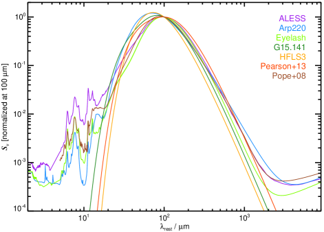
Figure 4.— The SED templates used here to determine photometric redshifts, normalized in flux density at 100-$\mu$m. The HFLS3 and Arp 220 SEDs are relatively blue for typical DSFGs, giving us a range of plausibly representative templates.

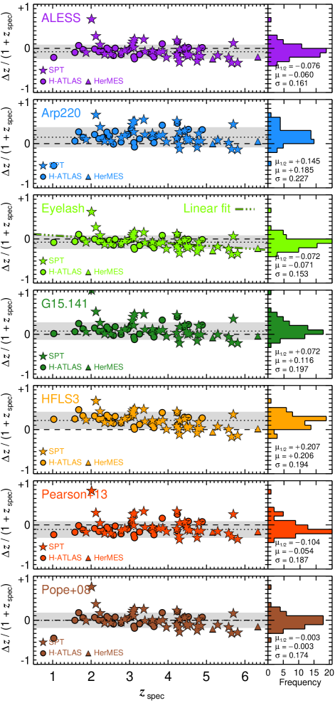
Figure 5.— Difference, $(z_{\rm phot}-z_{\rm spec})/(1+z_{\rm spec})$ or $\Delta z/(1+z_{\rm spec})$, as a function of $z_{\rm spec}$, between photometric redshifts determined using the SED templates shown in Fig. 4 and the spectroscopic redshifts, $z_{\rm spec}$, determined via detections of CO using broadband spectrometers for 69 bright DSFGs. We employed the available SPIRE photometric measurements and all additional photometry out to 1 mm, as tabulated by Ivison et al. (2010); Riechers et al. (2013); Robson et al. (2014); Bussmann et al. (2013); Weiß et al. (2013); Asboth et al. (2016) and Strandet et al. (2016). Approximately the same trend can be seen in each panel. A linear fit of the form $\Delta z/(1+z_{\rm spec})\propto-0.059\times z_{\rm spec}$, which is typical, is shown in the Cosmic Eyelash panel. The statistics noted in each panel illustrate the systematic underestimates or overestimates of $z_{\rm phot}$ found using the relevant SED templates, and the degree of scatter. It is worth noting that the redshifts of the templates are recovered accurately, showing that the process works well, e.g. in the HFLS3 panel, HFLS3 itself can be seen at $z=6.3$ with $\Delta z/(1+z_{\rm spec})=0$. The outlier at $z\sim 2$ is discussed in §4.2.2. On the basis of these statistics we discontinue using the Arp 220, G15.141, HFLS3 and Pearson et al. template SEDs in future analyses.

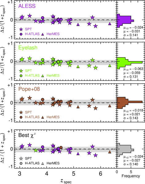
Figure 6.— Difference, $\Delta z/(1+z_{\rm spec})$, as a function of $z_{\rm spec}$, between photometric redshifts determined using the three SEDs shown to be the most effective templates in Fig. 5 and the spectroscopic redshifts, $z_{\rm spec}$, determined via detections of CO using broadband spectrometers for 25 ultrared DSFGs that match the color requirements of our sample here, drawn from this paper, from Weiß et al. (2013), Riechers et al. (2013), Asboth et al. (2016) and Strandet et al. (2016). As in Fig. 5, we employed the available SPIRE photometric measurements and all additional photometry out to 1 mm. The statistics noted in each panel show that the systematic underestimates or overestimates of $z_{\rm phot}$ found using the relevant SED templates are small, as is the scatter. The lower panel shows $\Delta z/(1+z_{\rm spec})$ for the template that yields the lowest $\chi^{2}$ for each ultrared DSFG, this being the approach we adopt hereafter to determine the redshift distribution of our full sample. The scatter in this lower panel represents the minimum systematic uncertainty in photometric redshift since these sources typically have higher S/N photometry than our faint, ultrared DSFG candidates.

For the first method, the distribution of measured redshifts and their associated uncertainties are governed by the choice of template SEDs, where adopting a broad range of SEDs makes more sense in some situations than in others. Blindly employing the second method offers less understanding of the potential systematics and uncertainties.

To characterize the systematics and overall uncertainties, we adopt seven well-sampled SEDs, all potentially representative of distant DSFGs: those for HFLS3, Arp 220, which are both relatively blue for DSFGs, plus those for the Cosmic Eyelash and G15.141, as well as synthesized templates from Pope et al. (2008), Pearson et al. (2013) and Swinbank et al. (2014, ALESS) – see Fig. 4. The Pearson et al. template was synthesised from 40 bright H-ATLAS sources with known spectroscopic redshifts and comprises two modified Planck functions, $T_{\rm hot}=46.9$ K and $T_{\rm cold}=23.9$ K, where the frequency dependence of the dust emissivity, $\beta$, is set to +2, and the ratio of cold to hot dust masses is 30.1:1. The lensed source, G15.141, is modelled using two greybodies with parameters taken from Lapi et al. (2011), $T_{\rm hot}=60$ K and $T_{\rm cold}=32$ K, $\beta=+2$ and the ratio of cold to hot dust masses of 50:1. Fig. 4 shows the diversity of these SEDs in the rest frame, normalized in flux density at 100 $\mu$m.

4.2.1 Training

Before we use these SED templates to determine the redshifts of our ultrared DSFGs, we want to estimate any systematic redshift uncertainties and reject any unsuitable templates, thereby ‘training’ our technique. To accomplish this, the SED templates were fitted to the available photometry for 69 bright DSFGs with SPIRE ($S_{250},S_{350},S_{500}$) and $S_{870}$ photometric measurements, the latter typically from the Submillimeter Array (Bussmann et al., 2013), and spectroscopic redshifts determined via detections of CO using broadband spectrometers (e.g. Weiß et al., 2013; Riechers et al., 2013; Asboth et al., 2016; Strandet et al., 2016). We used accurate filter transmission profiles in each case, searching for minima in the $\chi^{2}$ distribution over $0<z_{\rm phot}<10$, ignoring possible contamination of the various filters passbands by bright spectral lines such as [C ii] (Smail et al., 2011).

The differences between photometric redshifts estimated in this way and the measured spectroscopic redshifts for these 69 bright DSFGs were quantified using the property $(z_{\rm phot}-z_{\rm spec})/(1+z_{\rm spec})$, or $\Delta z/(1+z_{\rm spec})$ hereafter.

Fig. 5 shows the outcome when our seven SED templates are used to determine photometric redshifts for the 69 bright DSFGs with spectroscopic redshifts. We might have expected that the Pearson et al. template would yield the most accurate redshifts for this sample, given that it was synthesized using many of these same galaxies, but seemingly the inclusion of galaxies with optical spectroscopic redshifts during its construction has resulted in a slightly redder SED than the average for those DSFGs with CO spectroscopic redshifts, resulting in mean and median offsets, $\mu=-0.062$ and $\mu_{\rm 1/2}=-0.116$, with an r.m.s. scatter, $\sigma=0.187$. While the Pearson et al. template fares better than those of Arp 220, G15.141 and HFLS3, which have both higher offsets and higher scatter, as well as a considerable fraction of outliers (defined as those with $|\Delta z/(1+z_{\rm spec})|>0.3$), at this stage we discontinued using these four SEDs in the remainder of our analysis. We retained the three SED templates with $|\mu_{1/2}|<0.1$ and fewer than 10% outliers for the following important sanity check.

4.2.2 Sanity check

For this last test we employed the 25 ultrared DSFGs that match the color requirements of our ultrared sample. Their spectroscopic redshifts have been determined via detections of CO using broadband spectrometers, typically the 3-mm receivers at ALMA and NOEMA, drawn partly from the sample in this paper (see Fudamoto et al., 2016, for the spectroscopic follow-up) but mainly from from the literature (Cox et al., 2011; Weiß et al., 2013; Riechers et al., 2013; Asboth et al., 2016; Strandet et al., 2016).

Without altering our redshift-fitting procedure, we employed the available SPIRE photometric measurements together with all additional photometry out to 1 mm. For each source we noted the redshift and the template with the best $\chi^{2}$. Fig. 6 shows $\Delta z/(1+z_{\rm spec})$ as a function of $z_{\rm spec}$ and we can see that the Cosmic Eyelash and the synthesized templates from Swinbank et al. (ALESS) and Pope et al. have excellent predictive capabilities, with $|\mu_{1/2}|\mathrel{\raise 1.50696pt\hbox{$\scriptstyle<$}\kern-6.00006pt\lower 1.72218pt\hbox{{$\scriptstyle\sim$}}}0.06$ and $\sigma\sim 0.14$.

The lower panel of Fig. 6 shows $\Delta z/(1+z_{\rm spec})$ versus $z_{\rm spec}$ for the SED template that yields the best $\chi^{2}$ for each ultrared DSFG, where $\mu_{1/2}=-0.024$. The scatter seen in this plot is representative of the minimum systematic uncertainty in determining photometric redshifts for ultrared galaxies, $\sigma\sim 0.14$, given that the photometry for these brighter sources tends to be of a relatively high quality. Despite a marginally higher scatter than the best individual SED templates, we adopt the photometric redshifts with the lowest $\chi^{2}$ values hereafter.

4.2.3 The effect of the CMB

We have quantified the well-known effect of the CMB on the SED shape (da Cunha et al., 2013; Zhang et al., 2016) by using a dual-greybody 30 k + 60 k parameterization of the Cosmic Eyelash – the prescription of Ivison et al. (2010). At $z=2.3$, the Cosmic Eyelash is affected negligably by the CMB effect – of the two greybodies, the coolest is affected most, and it changes by just $\sim 4$ mK compared with $z=0$. We therefore ignore this and modify the parameterized $z=2.3$ SED to account for the effect of the CMB at progressively higher redshifts, then fit the unmodified Cosmic Eyelash SED to monochromatic flux densities drawn from these modified SEDs at $\lambda_{\rm obs}=250$, 350, 500 and 870 $\mu$m. The CMB effect causes us to underestimate $(1+z)$ by 0.03, 0.05, 0.10 and 0.18 at $z=4$, 6, 8 and 10. Thus, the effect is small, even at the highest plausible redshifts; moreover, since the effect biases our redshifts to lower values, our estimate of the space density of ultrared DSFGs at $z>4$ presented in §4.3 will be biased lower rather than higher.

4.2.4 Redshift trends

As an aside, a trend — approximately the same trend in each case — can be seen in each panel of Figs 5–6, with $\Delta z/(1+z_{\rm spec})$ decreasing numerically with increasing redshift. The relationship takes the form $\Delta z/(1+z_{\rm spec})\propto-0.059_{-0.014}^{+0.016}\times z_{\rm spec}$ for the Cosmic Eyelash, and a consistent trend is seen for the other SED templates. Were we to correct for this trend, the typical scatter in $\Delta z/(1+z_{\rm spec})$ would fall to $\sim 0.10$. This effect is much stronger than can be ascribed to the influence of the CMB and betrays a link between redshift and $T_{\rm dust}$, which in turn may be related to the relationship between redshift and $L_{\rm IR}$ seen by Symeonidis et al. (2013), though disentangling the complex relationships between $T_{\rm dust}$, $M_{\rm dust}$, $L_{\rm IR}$, starburst size and redshift is extraordinarily challenging, even if the cross-section to gravitational lensing were constant with distance, which it is not (see §4.3). By considering a greybody at the temperature of each of the templates in our library, we can deduce that an offset between the photometric and spectroscopic redshifts corresponds to a change in dust temperature of

$$\Delta T_{\rm dust}=T_{\rm dust}^{\rm grey}\left(\frac{1+z_{\rm phot}}{1+z{{}_{\rm spec}}}-1\right),$$ (1)

where $\Delta T_{\rm dust}$ is difference between the dust temperature of the source and the temperature of the template SED, $T_{\rm dust}^{\rm SED}$. Using the offset between the photometric and spectroscopic redshifts for the Cosmic Eyelash template, we estimate that the typical dust temperature of the sources in our sample becomes warmer on average by $9.4_{-3.3}^{+4.8}$ k as we move from $z=2$ ($-0.7$ k) to $z=6$ ($+8.7$ k). We find consistent results for the Pope et al. and ALESS template SEDs, where $\Delta T_{\rm dust}=7.5_{-3.1}^{+4.0}$ k and $7.1_{-3.0}^{+3.9}$ k, respectively. We do not reproduce the drop of 10 k between low and high redshift reported by Symeonidis et al. (2013) — quite the reverse, in fact. This may be related to the higher fraction of gravitationally lensed (and thus intrisically less luminous) galaxies expected in the bright sample we have used here to calibrate and test our photometric redshift technique (§4.3). As with the CMB effect, the observed evolution in temperature with redshift predominantly biases our photometric redshifts to lower values, re-inforcing the conservative nature of our estimate of the space density of ultrared DSFGs at $z>4$.

It is also worth noting that the correlation between $L_{\rm IR}$ and redshift – discussed later in §4.2.6 and probably due in part to the higher flux density limits at $z>5$ – may mean that optical depth effects become more influential at the highest redshifts, with consequences for the evolution of DSFG SEDs that are difficult to predict.

4.2.5 Ultimate test of $z_{\rm phot}$ reliability

Finally, we employed the refined SED fitting procedure outlined above to determine the redshift distribution of our full sample of ultrared DSFGs.

As a final test of $z_{\rm phot}$ reliability, Fig. 7 shows the best-fitting photometric redshift for one of the sources, NGP$-$190387, for which we have secured a spectroscopic redshift using ALMA or NOEMA (Fudamoto et al., 2016) and in Fig. 8 we present the photometric redshifts of all of the six ultrared DSFGs for which we have determined secure spectroscopic redshifts.

We find $|\mu_{1/2}|=+0.08$ and $\sigma=0.06$, and the r.m.s. scatter around $\Delta z/(1+z_{\rm spec})=0$ is 0.08, consistent with expectations set by the scatter ($\sim 0.10$) seen earlier amongst the trend-corrected redshifts determined using the Cosmic Eyelash SED.

Figure 7.— SPIRE and SCUBA-2 photometry for one of our ultrared galaxies with a spectroscopic redshift, $z_{\rm spec}=4.42$ (Fudamoto et al., 2016), and the best fit to the data, $z=4.36^{+0.37}_{-0.26}$ in this case made using the ALESS SED template of Swinbank et al. (2014).

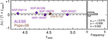
Figure 8.— Predictive power of our photometric redshifts, as judged using the six ultrared galaxies with spectroscopic redshifts from our sample (Fudamoto et al., 2016), on the same scale used earlier in Figs 5 and 6.

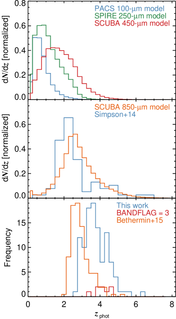
Figure 9.— Redshift histograms from Béthermin et al. (2015), representing a phenomenological model of galaxy evolution (Béthermin et al., 2012), with the expected redshift distributions for PACS at 100 $\mu$m ($S_{100}>9$ mJy), SPIRE at 250 $\mu$m ($S_{250}>20$ mJy), SCUBA-2 at 450 $\mu$m ($S_{450}>5$ mJy) in the upper panel. In the middle panel we show the Béthermin et al. redshift distribution predicted for SCUBA-2 at 850 $\mu$m ($S_{850}>4$ mJy), alongside the redshifts measured for the LABOCA 870-$\mu$m-selected LESS sample ($S_{870}>3.5$ mJy) by Simpson et al. (2014). In the lower panel we show the histogram of redshifts for our sample of ultrared galaxies, where for each galaxy we have adopted the redshift corresponding to the best $\chi^{2}$ fit, found with the SED templates used in Fig. 6. The subset (of eight galaxies) with bandflag=3, i.e. those selected from 500-$\mu$m residual maps, are shown in red. Our ultrared DSFGs typically lie $\delta z\approx 1.5$ redward of the 870-$\mu$m-selected sample. Comparison of the observed photometric redshift distribution for our ultrared DSFGs with that expected by the Béthermin et al. (2015) model (for sources selected with our flux limits and color criteria) reveals a significant mismatch.

4.2.6 Summary of $z_{\rm phot}$ and $L_{\rm IR}$ statistics

In Table 2, we list the photometric redshifts (and luminosities, measured in the rest-frame across 8–1000 $\mu$m) for each source in our sample, with uncertainties determined from a Monte Carlo treatment of the observed flux densities and their respective uncertainties.

Table 2Targets and their photometric redshift properties.

Nickname	$z$	$\log_{10}\left(L_{\textrm{FIR}}\right)$	Nickname	$z$	$\log_{10}\left(L_{\textrm{FIR}}\right)$
G09-47693	$3.12^{+0.39}_{-0.33}$	$13.01^{+0.14}_{-0.07}$	NGP-136610	$4.27^{+0.51}_{-0.51}$	$13.40^{+0.09}_{-0.12}$
G09-51190	$3.83^{+0.58}_{-0.48}$	$13.31^{+0.11}_{-0.12}$	NGP-158576	$3.15^{+0.36}_{-0.29}$	$13.00^{+0.12}_{-0.07}$
G09-59393	$3.70^{+0.35}_{-0.26}$	$13.28^{+0.05}_{-0.09}$	NGP-168885	$4.09^{+0.42}_{-0.30}$	$13.32^{+0.06}_{-0.08}$
G09-62610	$3.70^{+0.44}_{-0.26}$	$13.15^{+0.13}_{-0.06}$	NGP-172391	$3.27^{+0.34}_{-0.26}$	$13.08^{+0.09}_{-0.06}$
G09-64889	$3.48^{+0.48}_{-0.40}$	$13.10^{+0.09}_{-0.14}$	NGP-185990	$4.47^{+0.49}_{-0.37}$	$13.42^{+0.06}_{-0.06}$
G09-79552	$3.59^{+0.34}_{-0.26}$	$13.11^{+0.09}_{-0.06}$	NGP-190387	$4.36^{+0.37}_{-0.26}$	$13.49^{+0.05}_{-0.06}$
G09-79553	$3.66^{+0.39}_{-0.30}$	$13.08^{+0.11}_{-0.07}$	NGP-206987	$4.07^{+0.06}_{-0.60}$	$13.31^{+0.02}_{-0.13}$
G09-80620	$4.01^{+0.22}_{-0.78}$	$13.07^{+0.06}_{-0.19}$	NGP-239358	$3.47^{+0.52}_{-0.49}$	$13.09^{+0.10}_{-0.15}$
G09-80658	$4.07^{+0.09}_{-0.72}$	$13.20^{+0.03}_{-0.17}$	NGP-242820	$3.41^{+0.44}_{-0.30}$	$13.02^{+0.13}_{-0.06}$
G09-81106	$4.95^{+0.13}_{-0.73}$	$13.43^{+0.04}_{-0.13}$	NGP-244709	$3.48^{+0.42}_{-0.40}$	$13.14^{+0.07}_{-0.12}$
G09-81271	$4.62^{+0.46}_{-0.38}$	$13.39^{+0.05}_{-0.09}$	NGP-246114	$4.35^{+0.51}_{-0.46}$	$13.30^{+0.08}_{-0.10}$
G09-83017	$3.99^{+0.53}_{-0.34}$	$13.09^{+0.12}_{-0.08}$	NGP-247012	$4.59^{+0.16}_{-0.71}$	$13.21^{+0.04}_{-0.16}$
G09-83808	$5.66^{+0.06}_{-0.76}$	$13.51^{+0.02}_{-0.11}$	NGP-247691	$3.90^{+0.51}_{-0.45}$	$13.15^{+0.08}_{-0.13}$
G09-84477	$2.94^{+0.44}_{-0.39}$	$12.83^{+0.15}_{-0.09}$	NGP-248307	$3.59^{+0.36}_{-0.36}$	$12.96^{+0.10}_{-0.10}$
G09-87123	$4.28^{+0.52}_{-0.34}$	$13.17^{+0.12}_{-0.06}$	NGP-252305	$4.34^{+0.43}_{-0.38}$	$13.29^{+0.06}_{-0.09}$
G09-100369	$3.79^{+0.61}_{-0.46}$	$13.05^{+0.09}_{-0.13}$	NGP-255731	$4.94^{+0.73}_{-0.66}$	$13.30^{+0.09}_{-0.15}$
G09-101355	$4.20^{+0.70}_{-0.39}$	$13.03^{+0.16}_{-0.08}$	NGP-260332	$3.50^{+0.38}_{-0.29}$	$12.96^{+0.10}_{-0.08}$
G12-34009	$4.53^{+0.37}_{-0.31}$	$13.51^{+0.05}_{-0.06}$	NGP-284357	$4.99^{+0.44}_{-0.45}$	$13.40^{+0.05}_{-0.10}$
G12-42911	$4.33^{+0.31}_{-0.26}$	$13.45^{+0.05}_{-0.07}$	NGP-287896	$4.54^{+0.53}_{-0.37}$	$13.15^{+0.10}_{-0.09}$
G12-66356	$3.66^{+0.19}_{-0.72}$	$13.04^{+0.06}_{-0.19}$	NGP-297140	$3.41^{+0.57}_{-0.44}$	$12.91^{+0.15}_{-0.11}$
G12-77450	$3.53^{+0.46}_{-0.31}$	$12.99^{+0.14}_{-0.07}$	NGP-315918	$4.32^{+0.54}_{-0.33}$	$13.10^{+0.11}_{-0.07}$
G12-78339	$4.41^{+0.98}_{-0.70}$	$13.31^{+0.17}_{-0.18}$	NGP-315920	$3.88^{+0.33}_{-0.89}$	$13.05^{+0.07}_{-0.21}$
G12-78868	$3.58^{+0.34}_{-0.26}$	$13.04^{+0.08}_{-0.08}$	NGP-316031	$4.65^{+0.68}_{-0.47}$	$13.10^{+0.13}_{-0.07}$
G12-79192	$2.95^{+0.38}_{-0.36}$	$12.80^{+0.12}_{-0.12}$	SGP-28124	$3.93^{+0.08}_{-0.45}$	$13.65^{+0.02}_{-0.09}$
G12-79248	$6.43^{+0.81}_{-0.89}$	$13.76^{+0.11}_{-0.14}$	SGP-28124*	$3.80^{+0.02}_{-0.42}$	$13.61^{+0.00}_{-0.11}$
G12-80302	$3.06^{+0.39}_{-0.35}$	$12.83^{+0.12}_{-0.10}$	SGP-72464	$3.06^{+0.21}_{-0.19}$	$13.23^{+0.07}_{-0.05}$
G12-81658	$2.93^{+0.38}_{-0.42}$	$12.77^{+0.12}_{-0.14}$	SGP-93302	$3.91^{+0.27}_{-0.22}$	$13.46^{+0.04}_{-0.07}$
G12-85249	$2.87^{+0.37}_{-0.36}$	$12.70^{+0.11}_{-0.12}$	SGP-93302*	$3.79^{+0.24}_{-0.21}$	$13.43^{+0.04}_{-0.07}$
G12-87169	$3.26^{+0.51}_{-0.39}$	$12.85^{+0.13}_{-0.12}$	SGP-135338	$3.06^{+0.33}_{-0.26}$	$13.08^{+0.11}_{-0.04}$
G12-87695	$3.68^{+0.58}_{-0.53}$	$13.09^{+0.09}_{-0.14}$	SGP-156751	$2.93^{+0.24}_{-0.22}$	$12.97^{+0.08}_{-0.04}$
G15-21998	$2.91^{+0.20}_{-0.19}$	$13.10^{+0.06}_{-0.05}$	SGP-196076	$4.51^{+0.47}_{-0.39}$	$13.42^{+0.07}_{-0.06}$
G15-24822	$2.77^{+0.27}_{-0.27}$	$12.97^{+0.09}_{-0.08}$	SGP-208073	$3.48^{+0.40}_{-0.28}$	$13.18^{+0.06}_{-0.08}$
G15-26675	$4.36^{+0.25}_{-0.21}$	$13.55^{+0.04}_{-0.05}$	SGP-213813	$3.49^{+0.40}_{-0.32}$	$13.15^{+0.07}_{-0.10}$
G15-47828	$3.52^{+0.50}_{-0.39}$	$13.20^{+0.09}_{-0.11}$	SGP-219197	$2.94^{+0.25}_{-0.24}$	$13.03^{+0.08}_{-0.07}$
G15-64467	$3.75^{+0.55}_{-0.49}$	$13.15^{+0.09}_{-0.14}$	SGP-240731	$2.70^{+0.27}_{-0.25}$	$12.88^{+0.10}_{-0.09}$
G15-66874	$4.07^{+0.57}_{-0.49}$	$13.30^{+0.10}_{-0.11}$	SGP-261206	$5.03^{+0.58}_{-0.47}$	$13.64^{+0.09}_{-0.10}$
G15-82412	$3.96^{+0.15}_{-0.70}$	$13.20^{+0.04}_{-0.16}$	SGP-304822	$4.33^{+0.63}_{-0.51}$	$13.41^{+0.12}_{-0.12}$
G15-82684	$3.65^{+0.38}_{-0.25}$	$13.13^{+0.11}_{-0.06}$	SGP-310026	$3.12^{+0.38}_{-0.31}$	$12.97^{+0.12}_{-0.07}$
G15-83543	$3.53^{+0.42}_{-0.34}$	$13.05^{+0.12}_{-0.09}$	SGP-312316	$3.17^{+0.41}_{-0.32}$	$12.94^{+0.12}_{-0.08}$
G15-83702	$3.27^{+0.39}_{-0.36}$	$12.90^{+0.12}_{-0.12}$	SGP-317726	$3.69^{+0.39}_{-0.30}$	$13.20^{+0.06}_{-0.10}$
G15-84546	$4.34^{+0.56}_{-0.53}$	$13.19^{+0.10}_{-0.14}$	SGP-354388	$5.35^{+0.56}_{-0.52}$	$13.68^{+0.08}_{-0.08}$
G15-85113	$3.40^{+0.37}_{-0.34}$	$12.90^{+0.09}_{-0.11}$	SGP-354388*	$5.43^{+0.84}_{-0.72}$	$13.69^{+0.12}_{-0.13}$
G15-85592	$3.39^{+0.49}_{-0.39}$	$12.89^{+0.15}_{-0.13}$	SGP-32338	$3.93^{+0.26}_{-0.24}$	$13.24^{+0.05}_{-0.04}$
G15-86652	$3.43^{+0.44}_{-0.35}$	$12.97^{+0.11}_{-0.09}$	SGP-380990	$2.84^{+0.22}_{-0.21}$	$12.84^{+0.06}_{-0.07}$
G15-93387	$3.24^{+0.50}_{-0.33}$	$12.87^{+0.12}_{-0.08}$	SGP-381615	$2.98^{+0.29}_{-0.29}$	$12.91^{+0.09}_{-0.09}$
G15-99748	$3.98^{+0.25}_{-0.79}$	$13.06^{+0.05}_{-0.20}$	SGP-381637	$3.30^{+0.28}_{-0.25}$	$13.06^{+0.08}_{-0.07}$
G15-105504	$3.43^{+0.64}_{-0.53}$	$12.87^{+0.16}_{-0.13}$	SGP-382394	$2.96^{+0.29}_{-0.26}$	$12.84^{+0.08}_{-0.08}$
NGP-63663	$3.08^{+0.23}_{-0.22}$	$13.11^{+0.08}_{-0.06}$	SGP-383428	$3.08^{+0.33}_{-0.30}$	$12.88^{+0.10}_{-0.09}$
NGP-82853	$3.66^{+0.06}_{-0.61}$	$13.17^{+0.02}_{-0.15}$	SGP-385891	$3.70^{+0.29}_{-0.24}$	$13.20^{+0.07}_{-0.06}$
NGP-101333	$3.53^{+0.34}_{-0.27}$	$13.30^{+0.06}_{-0.09}$	SGP-386447	$4.89^{+0.78}_{-0.73}$	$13.41^{+0.13}_{-0.17}$
NGP-101432	$3.65^{+0.36}_{-0.28}$	$13.31^{+0.05}_{-0.10}$	SGP-392029	$3.42^{+0.47}_{-0.32}$	$13.00^{+0.13}_{-0.06}$
NGP-111912	$3.27^{+0.36}_{-0.26}$	$13.09^{+0.10}_{-0.06}$	SGP-424346	$3.99^{+0.45}_{-0.39}$	$12.95^{+0.10}_{-0.10}$
NGP-113609	$3.43^{+0.34}_{-0.20}$	$13.22^{+0.09}_{-0.04}$	SGP-433089	$3.60^{+0.08}_{-0.62}$	$13.11^{+0.01}_{-0.13}$
NGP-126191	$4.33^{+0.45}_{-0.46}$	$13.37^{+0.07}_{-0.08}$	SGP-499646	$4.68^{+0.49}_{-0.34}$	$13.14^{+0.10}_{-0.05}$
NGP-134174	$2.98^{+0.34}_{-0.31}$	$12.98^{+0.12}_{-0.07}$	SGP-499698	$4.22^{+0.39}_{-0.38}$	$13.00^{+0.09}_{-0.11}$
NGP-136156	$3.95^{+0.06}_{-0.57}$	$13.33^{+0.01}_{-0.12}$	SGP-499828	$3.88^{+0.49}_{-0.41}$	$12.88^{+0.10}_{-0.09}$

We present a histogram of photometric redshifts for our sample of ultrared galaxies in Fig. 9, where for each galaxy we have adopted the redshift corresponding to the best $\chi^{2}$ fit, found with the SED templates used in Fig. 6. In the upper panels of Fig. 9 we show redshift histograms from Béthermin et al. (2015), representing a phenomenological model of galaxy evolution (Béthermin et al., 2012), with the expected redshift distributions for PACS at 100 $\mu$m ($S_{100}>9$ mJy), SPIRE at 250 $\mu$m ($S_{250}>20$ mJy), SCUBA-2 at 450 $\mu$m ($S_{450}>5$ mJy), SCUBA-2 at 850 $\mu$m ($S_{850}>4$ mJy), cf. the redshifts measured for the LABOCA 870-$\mu$m-selected LESS sample ($S_{870}>3.5$ mJy) by Simpson et al. (2014).

Our Herschel-selected ultrared galaxies span $2.7<z_{\rm phot}<6.4$, and typically lie $\delta z\approx 1.5$ redward of the 870-$\mu$m-selected sample, showing that our technique can be usefully employed to select intense, dust-enshrouded starbursts at the highest redshifts. We find that $33\pm 6$% of our full sample (1-$\sigma$ errors, Gehrels, 1986) and $63_{-24}^{+20}$% of our bandflag=3 subset (see overlaid red histogram in lower panel of Fig. 9) lie at $z_{\rm phot}>4$. In an ultrared sample comprised largely of faint 500-$\mu$m risers, we find a median value of $\hat{z}_{\rm phot}=3.66$, a mean of 3.79 and an interquartile range, 3.30–4.27. This supports the relation between the SED peak and redshift observed by Swinbank et al. (2014), who found median redshifts of $2.3\pm 0.2$, $2.5\pm 0.3$ and $3.5\pm 0.5$ for 870-$\mu$m-selected DSFGs with SEDs peaking at 250, 350 and 500 $\mu$m.

Comparison of the observed photometric redshift distribution for our ultrared DSFGs with that expected by the Béthermin et al. (2015) model (for sources selected with our flux density limits and color criteria) reveals a significant mismatch, with the model histogram skewed by $\delta z\approx 1$ bluewards of the observed distribution. This suggests that our current understanding of galaxy evolution is incomplete, at least with regard to the most distant, dust-enshrouded starbursts, plausibly because of the influence of gravitational lensing, although the Béthermin et al. model does include a simple treatment of this effect. This issue will be addressed in a forthcoming paper in which we present high-resolution ALMA imaging (Oteo et al., 2016b, see also Fig. 10).

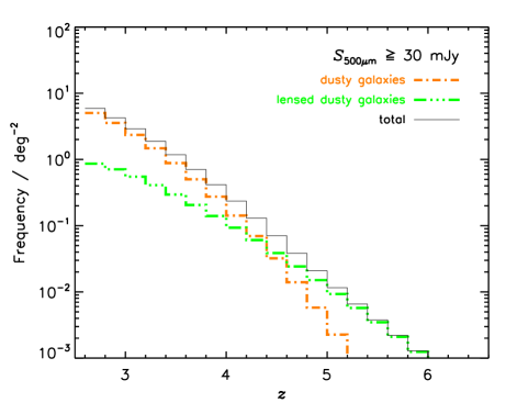
Figure 10.— Redshift distribution of $S_{500}>30$-mJy sources from the physical model of Cai et al. (2013) which provides a good fit to a broad variety of data, including the IR luminosity functions determined observationally by Gruppioni et al. (2013) at several redshifts up to $z\sim 4$ (see also Figure 1 of Bonato et al., 2014). The dot-dashed green histogram and the dot-dashed orange histogram show the contributions of strongly lensed (magnification, $\mu\geq 2$) and unlensed galaxies, respectively, while the black histogram shows the total. The distribution of lensed galaxies was computed using the SISSA model (Lapi et al., 2012). Although strongly lensed galaxies are a minor fraction of all galaxies with $S_{500}>30\,$mJy, they become common at $z>4$ due to the combined effect of the increase with redshift of the optical depth to lensing and the magnification bias. This will be addressed in a forthcoming paper, in which we present high-resolution ALMA imaging (Oteo et al., 2016b).

The corresponding 8–1000-$\mu$m luminosities for our sample of ultrared DSFGs, in the absence of gravitational lensing, range from $5.0\times 10^{12}$ to $5.8\times 10^{13}$ L_⊙, a median of $1.3\times 10^{13}$ L_⊙ and an interquartile range of $9.7\times 10^{12}$ to $2.0\times 10^{13}$ L_⊙.

Fig. 10 demonstrates that the influence of gravitational lensing cannot be wholly ignored. Although strongly lensed galaxies are a minor fraction of all galaxies with $S_{500}>30\,$mJy, they become more common at $z>4$ due to the combined effect of the increase with redshift of the optical depth to lensing and the magnification bias. This will be addressed in a forthcoming paper, in which we present high-resolution ALMA imaging (Oteo et al., 2016b).

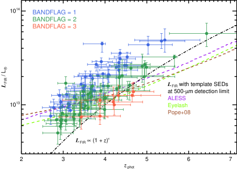
Figure 11.— $L_{\rm IR}$ as a function of $z_{\rm phot}$ for our sample, color-coded by bandflag, with the $S_{500}>30$-mJy detection limits shown for our three best SED templates, and luminosity evolution of the form $\propto(1+z)^{4}$ illustrated. We see that the bandflag $=1$, 2 and 3 galaxies lie in distinct regions, as one might expect. The least luminous galaxies at any redshift are those detected only in the 500-$\mu$m filter, since in the SPIRE maps with the lowest spatial resolution they suffer considerably more flux boosting and blending. The growing gap between the galaxies and the expected detection limits at $z>5$ is potentially interesting.

In Fig. 11 we show how the 8–1000-$\mu$m luminosities of our ultrared DSFGs behave as a function of redshift, to help explain the shape of our redshift distribution, and any biases. The $S_{500}>30$-mJy detection limit for our three best SED templates are shown, as well as luminosity evolution of the form $(1+z)^{4}$, scaled arbitrarily. The different bandflag categories separate from one another, as one might expect, where the least luminous galaxies at any redshift are those detected only in the 500-$\mu$m filter, having suffered considerably more flux boosting and blending in the SPIRE maps with the lowest spatial resolution. The growing gap between the ultrared DSFGs and the expected detection limits at $z>5$ is potentially interesting, possibly reflecting the relatively low number of bandflag $=3$ sources in our sample and the growing influence of multi-band detections at the highest redshifts.

4.3. The space density of distant DSFGs

With photometric redshift estimates for each of the sources in our sample we can now set a lower limit on the space density, $\rho$, of $S_{500}>30$-mJy ultrared DSFGs that lie at $z>4$. As summarised in S4.2.6, we find that $33\pm 6$% of the sources in our sample lie in the range $4<z<6$ and the space density of these DSFGs is

$$\rho=\frac{N_{z}}{\mathcal{C}\,V_{\rm obs}}\times\frac{t_{\rm obs}}{t_{\rm burst}}\,\,\,\,\,\,\,{\rm Mpc}^{-3},$$ (2)

where $N_{z}$ represents the number of sources within $4<z<6$, $V_{\rm obs}$ is the comoving volume contained within the redshift range considered, $t_{\rm obs}/t_{\rm burst}$ is a duty-cycle correction, since the ongoing, obscured starburst in DSFGs has a finite duration, where $t_{\rm burst}\approx 100$ Myr is in agreement with their expected gas depletion times (Ivison et al., 2011; Bothwell et al., 2013) but is uncertain at the $\approx 2\times$ level. $\mathcal{C}$ is the completeness correction required for our sample, as discussed at length in §2.3–2.4. $V_{\rm obs}$ is the comoving volume contained within $4<z<6$, given by

$$V_{\rm obs}=\frac{4\pi}{3}\int_{z=4}^{z=6}\frac{c/H_{\rm 0}}{\sqrt{\Omega_{\rm M}(1+z^{\prime})^{3}+\Omega_{\rm V}}}dz^{\prime}\,\,\,\,\,\,\,{\rm Mpc}^{3}$$ (3)

(Hogg, 1999), which we scale by the fractional area of sky that was surveyed, $\approx 600$ deg², or $\approx 1.5$%.

Applying these corrections we estimate that ultrared, DSFGs at $z>4$ have a space density of $\approx 6\times 10^{-7}$ Mpc^-3. Our work represents the first direct measurement of the space density of $z>4$ DSFGs at such faint flux-density limits and as such it is not possible to make a direct comparison with previous studies in the literature. For example, Asboth et al. (2016) recently presented the number counts of ultrared, 500–$\mu$m–selected DSFGs, identified in the 274-deg² HerMES Large Mode Survey (HELMS). However, the Asboth et al. galaxies are considerably brighter than ours, meaning a significant fraction will be gravitationally lensed, and they lack redshift estimates, so it is impossible to judge meaningfully whether their source density is consistent with the results presented here.

4.4. Relationship of DSFGs with other galaxy populations

It has been suggested by a number of authors (e.g. Simpson et al., 2014; Toft et al., 2014; Ikarashi et al., 2015) that high-redshift DSFGs may be the progenitors of the population of massive, quiescent galaxies that have been uncovered in near-IR surveys (e.g. van Dokkum et al., 2008; Newman et al., 2012; Krogager et al., 2014; Straatman et al., 2014). These galaxies are generally found to be extremely compact which, when taken in conjunction with their high stellar masses, $\approx 10^{11}$ M_⊙, and high redshifts, $z\mathrel{\raise 1.50696pt\hbox{$\scriptstyle>$}\kern-6.00006pt\lower 1.72218pt\hbox{{$\scriptstyle\sim$}}}2$, motivates the idea that the stellar component was formed largely during an intense starburst phase, enshrouded in dust.

Is the comoving space density of ultrared, high-redshift DSFGs consistent with that of massive, high-redshift, quiescent galaxies? As discussed earlier, the $4<z<6$ DSFGs presented in this work have a comoving space density of $\approx 6\times 10^{-7}$ Mpc^-3. As a comparison, we use the galaxies in the sample presented by Straatman et al. (2014), which were classified as quiescent via $UVJ$ selection (e.g. Labbé et al., 2005) and are drawn from a mass-limited sample ($>4\times 10^{10}$ M_⊙). These galaxies were selected to lie in the redshift range $3.4<z<4.2$ and were estimated to have a median stellar age of $\approx 0.8$ Gyr, indicating a typical formation epoch of $z\approx 5$, making them an ideal match to our sample of $4<z<6$ DSFGs.

The quiescent sources presented by Straatman et al. (2014) have a comoving space density of $\approx 2\times 10^{-5}$ Mpc^-3, $\approx 30\times$ more numerous than the sample of DSFGs presented here. Even at $M_{\rm stars}\mathrel{\raise 1.50696pt\hbox{$\scriptstyle>$}\kern-6.00006pt\lower 1.72218pt\hbox{{$\scriptstyle\sim$}}}10^{11}$ M_⊙, Straatman et al. estimate a space density of $\approx 4\times 10^{-6}$ Mpc^-3 for their quiescent near-IR galaxies, still almost an order of magnitude higher than our $z>4$ DSFGs. This indicates clearly that $z>4$ DSFGs cannot account for the formation of massive, quiscent galaxies at $z\sim 3$–4 when selected at the flux-density levels we have been able to probe with Herschel. Even an infeasibly short duration of $\mathrel{\raise 1.50696pt\hbox{$\scriptstyle<$}\kern-6.00006pt\lower 1.72218pt\hbox{{$\scriptstyle\sim$}}}10$ Myr for the starburst phase of DSFGs is insufficient to bring the comoving space densities of the two populations into agreement, except at the very highest masses. Instead, our $S_{350}\approx S_{500}\approx 30$-mJy flux density limits are selecting the rarest, most FIR-bright objects on the sky — hyperluminous galaxies (e.g. Fu et al., 2013; Ivison et al., 2013) — which can form a galaxy with $\mathrel{\raise 1.50696pt\hbox{$\scriptstyle>$}\kern-6.00006pt\lower 1.72218pt\hbox{{$\scriptstyle\sim$}}}10^{11}$ M_⊙ of stars in $\mathrel{\raise 1.50696pt\hbox{$\scriptstyle<$}\kern-6.00006pt\lower 1.72218pt\hbox{{$\scriptstyle\sim$}}}100$ Myr, and/or less massive galaxies caught during a tremendously violent, short-lived phase, or gravitationally magnified by a chance alignment, populations that — even collectively — are considerably rarer than massive, high-redshift, quiescent galaxies.

The ALMACAL program of Oteo et al. (2016a) has shown that that $S_{870}\mathrel{\raise 1.50696pt\hbox{$\scriptstyle>$}\kern-6.00006pt\lower 1.72218pt\hbox{{$\scriptstyle\sim$}}}1$-mJy DSFGs with SFRs of $\approx 50$–100 M_⊙ yr^-1 are three orders of magnitude more common than our $z>4$ Herschel-selected DSFGs, such that $\approx 1$–2% of them lying at $z>4$ may account for the massive, quiescent near-IR-selected galaxies. Given the limited mapping speed of ALMA, even this fainter, more numerous DSFG population will be best accessed via a facility designed to obtain deep, wide-field imaging in passbands spanning 350 $\mu$m through 2 mm, either a large dish or a compact array equipped with focal-plane arrays.

We must therefore admit that although the progenitors of the most massive ($\mathrel{\raise 1.50696pt\hbox{$\scriptstyle>$}\kern-6.00006pt\lower 1.72218pt\hbox{{$\scriptstyle\sim$}}}10^{11}$-M_⊙) quiescent galaxies are perhaps just within our grasp, if we can push this color-selection technique further, the progenitors of the more general near-IR-selected quiescent galaxy population lie below the flux-density regime probed directly by Herschel. The progenitors of $z>6$ quasars, discussed in §1, remain similarly elusive: our ultrared DSFG space density is well matched, but we have yet to unveil any of the $z>6$ galaxies that may be hidden within our sample.

5. Conclusions

We have presented follow up SCUBA-2 and LABOCA imaging of a sample of 109 ultrared DSFGs with Herschel SPIRE colors of $S_{500}/S_{250}\geq 1.5$ and $S_{500}/S_{350}\geq 0.85$, thereby improving the accuracy of FIR-/submm-based photometric redshifts. After selecting the three SED templates most suitable for determining photometric redshifts, from a parent sample of seven, we performed two further sanity checks, looking for significant systematics and finding none, suggesting a high degree of accuracy. We then determine a median redshift, $\hat{z}_{\rm phot}=3.66$, and an interquartile range of $z_{\rm phot}=3.30$–4.27, with a median rest-frame 8–1000-$\mu$m luminosity, $\hat{L}_{\rm IR}=1.3\times 10^{13}$ L_⊙. We determine that $32\pm 5$% lie at $z_{\rm phot}>4$, and that the space density of such galaxies is $\approx 6\times 10^{-7}$ Mpc^-3.

Comparison of the observed photometric redshift distribution for our ultrared DSFGs with that expected by a phenomenological model of galaxy evolution reveals a significant mismatch, with the model skewed by $\delta z\approx 1$ bluewards of the observed redshift distribution.

Although the progenitors of the most massive ($\mathrel{\raise 1.50696pt\hbox{$\scriptstyle>$}\kern-6.00006pt\lower 1.72218pt\hbox{{$\scriptstyle\sim$}}}10^{11}$-M_⊙) near-IR-selected quiescent galaxies are perhaps just within our grasp, if we push this color-selection technique further, the progenitors of the more general near-IR-selected quiescent galaxy population lie below the flux-density regime probed directly by Herschel. Our ultrared DSFG space density is relatively well matched to that of $z>6$ quasars, but their progenitors remain elusive since we have yet to unveil any $z>6$ galaxies in our sample.

With this unique sample, we have substantially increased the number of $z>4$ dusty galaxies, partially fulfilling the promise of early predictions for the negative $K$ correction in the submm band (Blain & Longair, 1993). However, although we can claim considerable success in significantly enlarging the known sample of ultrared DSFGs at $z>4$, we must acknowledge that over half of our sources lie at $z<4$. Because of this, and the uncertain fraction of spurious sources in our parent ultrared DSFG catalog, we regard further refinement of the ultrared selection technique as both possible and necessary.

Finally, we draw attention to an interesting source, HATLAS J004223.5$-$334340 (SGP-354388), which we have dubbed the ‘Great Red Hope’ (or GRH). This system is resolved in our LABOCA and SCUBA-2 imaging, with a total 850-$\mu$m [870-$\mu$m] flux density of $58\pm 7$ [$64\pm 11$] mJy. In a 3-mm continuum map from ALMA covering $\approx 1$ arcmin² (Fudamoto et al., 2016), we see a number of discrete DSFGs (Oteo et al., 2016c), most of which display a single emission line at 98.4 GHz, an overdensity of galaxies that continues on larger scales, as probed by wide-field LABOCA imaging (Lewis et al., 2016). Photometric redshifts are challenging under these circumstances, given the confusion in the Herschel bands. Using the Swinbank et al. ALESS SED template with point-source flux densities suggests the lowest plausible redshift for these galaxies is $\approx 4.0$, while the method used throughout this work to measure flux densities gives $z_{\rm phot}\sim 5.4$. At anything like this distance, this is a remarkable cluster of ultrared DSFGs.

In this Appendix we present the Herschel SPIRE, JCMT/SCUBA-2 and APEX/LABOCA imaging of our red galaxy sample in the GAMA 9-hr, 12-hr and 15-hr fields, as well as the NGP and SGP fields. In each column, from left to right, we show 250-, 350-, 500- and 850-$\mu$m [870-$\mu$m for LABOCA] cut-out images, each $3^{\prime}\times 3^{\prime}$ and centered on the (labelled) galaxy. The 250- and 850-$\mu$m [870-$\mu$m] cut-out images have been convolved with 7^′′ and 13^′′ [19^′′] Gaussians, respectively. The 45^′′ aperture used to measure $S_{\rm tot}$ is shown. A 60^′′ aperture was also used but is not shown, to aid clarity. The annulus used to measure the background level is shown in the uppermost case (this is correspondingly larger for the 60^′′ aperture – see §4.1). SPIRE images are displayed from $-6$ to +60 mJy beam^-1; SCUBA and LABOCA images are displayed from $-3$ to +30 mJy beam^-1; both scales are relative to the local median. North is up and East is left.

 

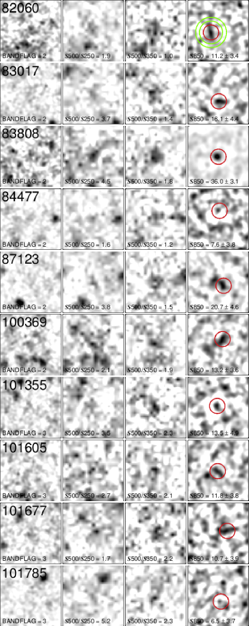
Figure 1.— Targets in the GAMA 9-hr field, observed by SCUBA-2.

 

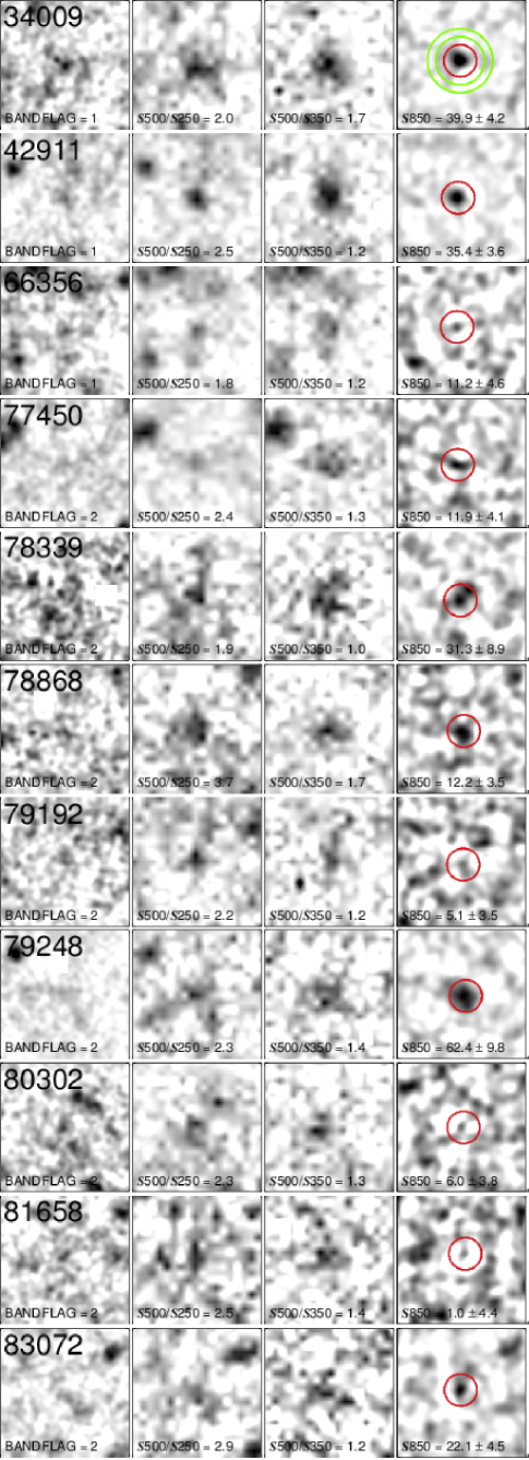
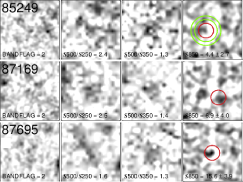
Figure 2.— Targets in the GAMA 12-hr field, observed by SCUBA-2.

 

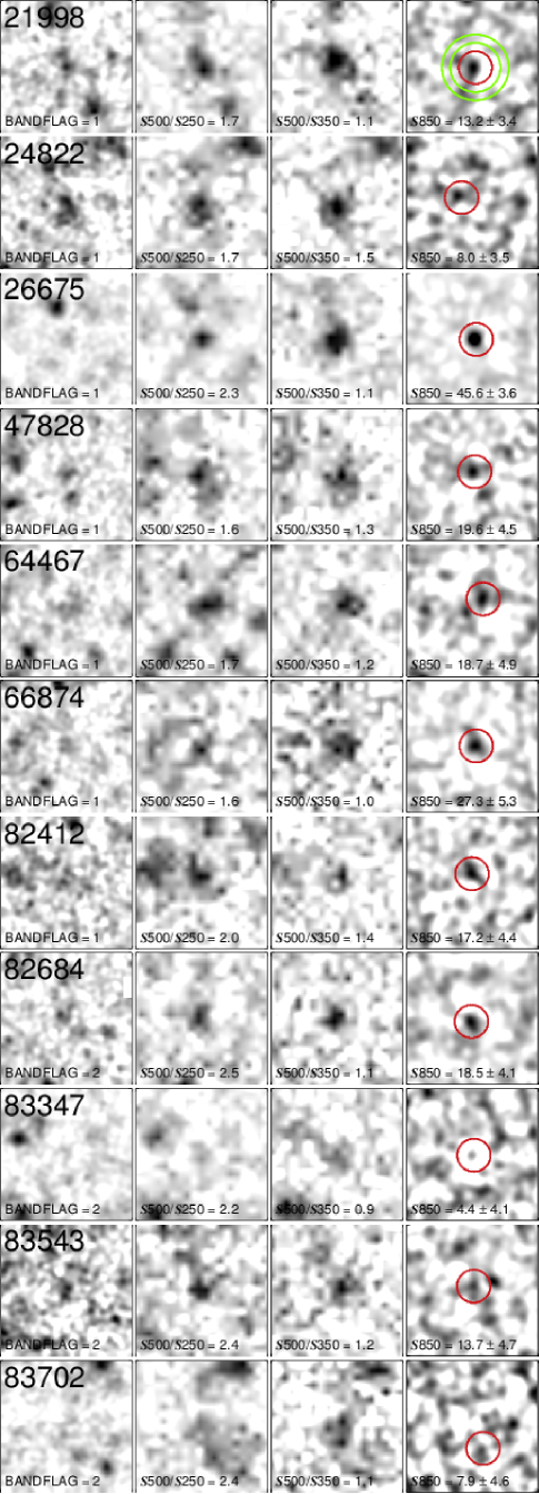
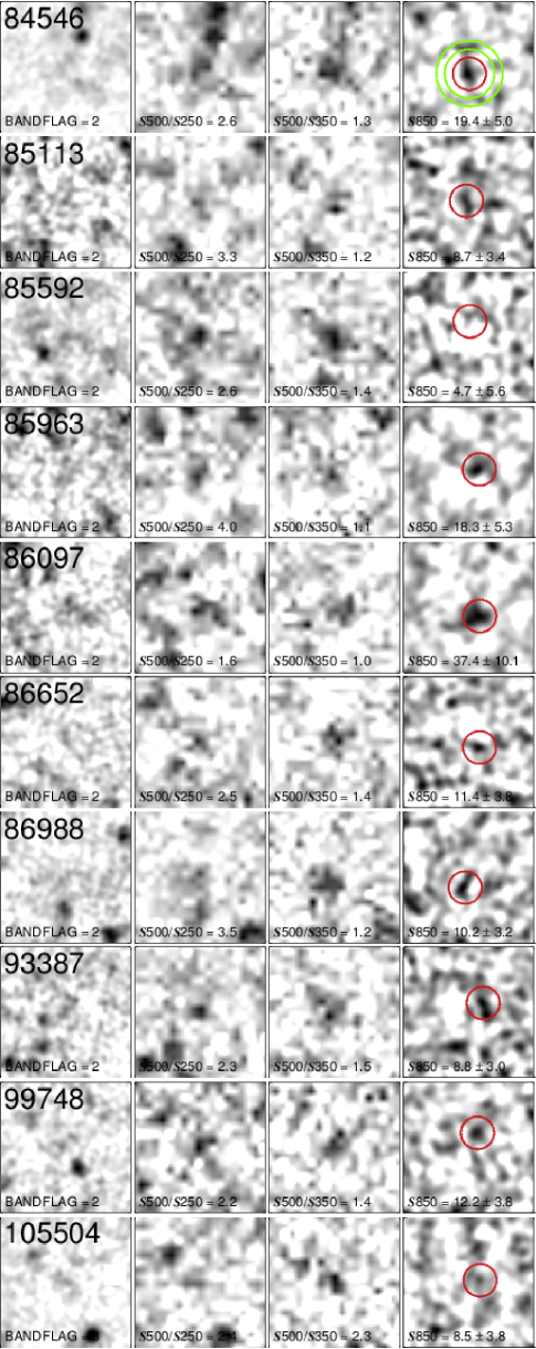
Figure 3.— Targets in the GAMA 15-hr field, observed by SCUBA-2.

 

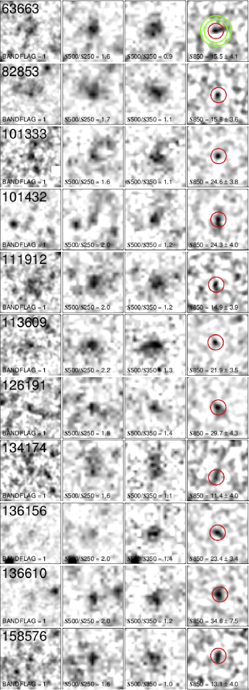
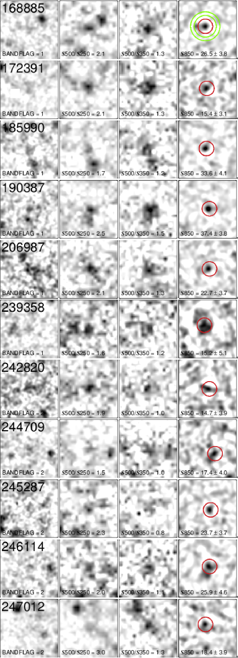
Figure 4.— Targets in the NGP field, observed by SCUBA-2.

 

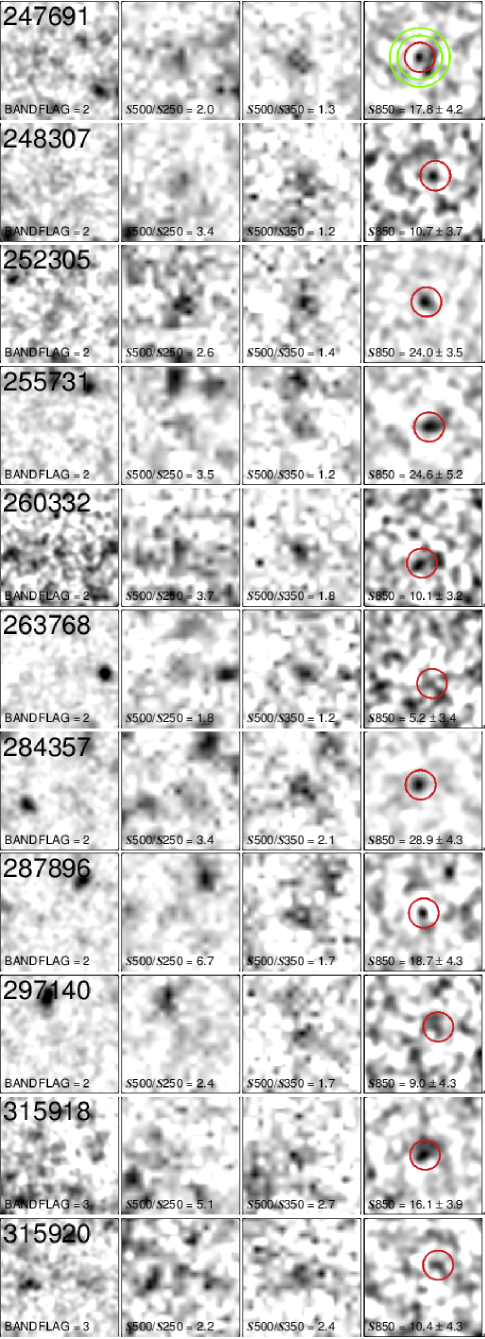
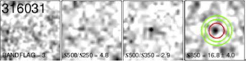
Figure 4.— Cont…

 

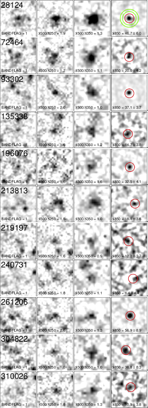
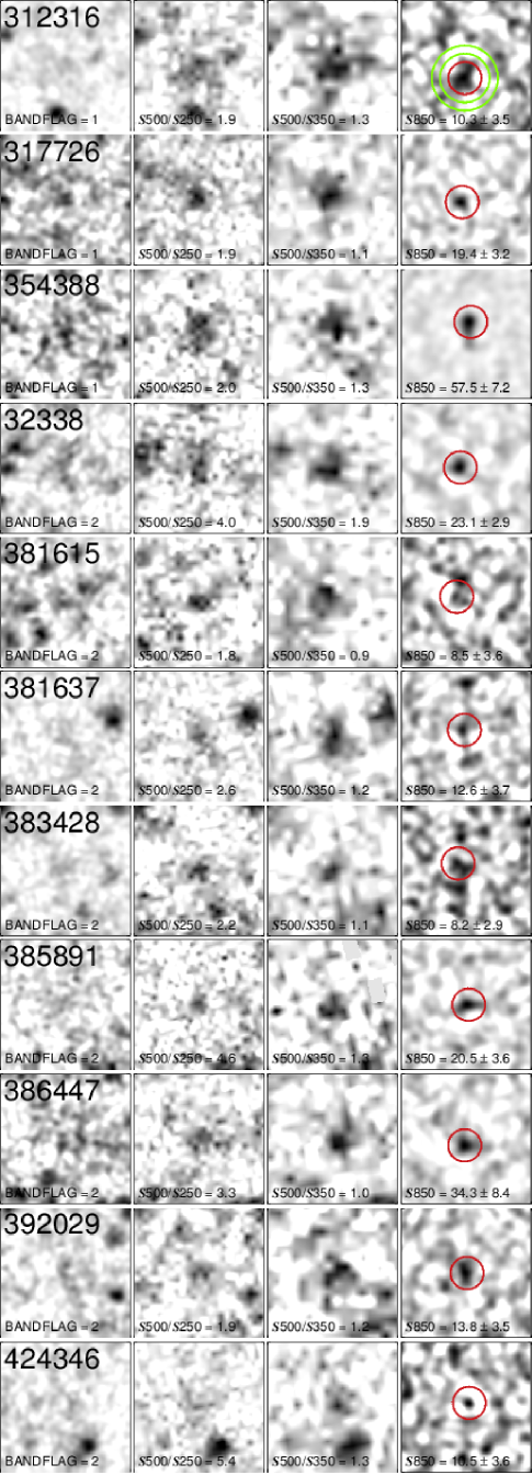
Figure 5.— Targets in the SGP field, observed by SCUBA-2.

 

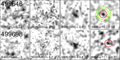
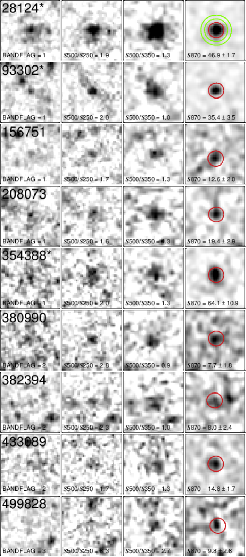
Figure 5.— Left: Cont… Right: Targets in the SGP field, observed by LABOCA.

References

- Aretxaga et al. (2003) Aretxaga, I., Hughes, D. H., Chapin, E. L., et al. 2003, MNRAS, 342, 759
- Asboth et al. (2016) Asboth, V., Conley, A., Sayers, J., et al. 2016, MNRAS, 462, 1989
- Barger et al. (1998) Barger, A. J., Cowie, L. L., Sanders, D. B., et al. 1998, Nature, 394, 248
- Béthermin et al. (2015) Béthermin, M., De Breuck, C., Sargent, M., & Daddi, E. 2015, A&A, 576, L9
- Béthermin et al. (2012) Béthermin, M., Daddi, E., Magdis, G., et al. 2012, ApJ, 757, L23
- Blain & Longair (1993) Blain, A. W., & Longair, M. S. 1993, MNRAS, 264, 509
- Bonato et al. (2014) Bonato, M., Negrello, M., Cai, Z.-Y., et al. 2014, MNRAS, 438, 2547
- Bothwell et al. (2013) Bothwell, M. S., Smail, I., Chapman, S. C., et al. 2013, MNRAS, 429, 3047
- Bussmann et al. (2013) Bussmann, R. S., Pérez-Fournon, I., Amber, S., et al. 2013, ApJ, 779, 25
- Cai et al. (2013) Cai, Z.-Y., Lapi, A., Xia, J.-Q., et al. 2013, ApJ, 768, 21
- Chapin et al. (2013) Chapin, E. L., Berry, D. S., Gibb, A. G., et al. 2013, MNRAS, 430, 2545
- Chapin et al. (2011) Chapin, E. L., Chapman, S. C., Coppin, K. E., et al. 2011, MNRAS, 411, 505
- Chapman et al. (2003) Chapman, S. C., Blain, A. W., Ivison, R. J., & Smail, I. R. 2003, Nature, 422, 695
- Conley et al. (2011) Conley, A., Cooray, A., Vieira, J. D., et al. 2011, ApJ, 732, L35
- Cox et al. (2011) Cox, P., Krips, M., Neri, R., et al. 2011, ApJ, 740, 63
- da Cunha et al. (2013) da Cunha, E., Groves, B., Walter, F., et al. 2013, ApJ, 766, 13
- Dempsey et al. (2013) Dempsey, J. T., Friberg, P., Jenness, T., et al. 2013, MNRAS, 430, 2534
- Dowell et al. (2014) Dowell, C. D., Conley, A., Glenn, J., et al. 2014, ApJ, 780, 75
- Eales et al. (2010) Eales, S., Dunne, L., Clements, D., et al. 2010, PASP, 122, 499
- Ellis et al. (2013) Ellis, R. S., McLure, R. J., Dunlop, J. S., et al. 2013, ApJ, 763, L7
- Engel et al. (2010) Engel, H., Tacconi, L. J., Davies, R. I., et al. 2010, ApJ, 724, 233
- Fan et al. (2001) Fan, X., Narayanan, V. K., Lupton, R. H., et al. 2001, AJ, 122, 2833
- Frayer et al. (2011) Frayer, D. T., Harris, A. I., Baker, A. J., et al. 2011, ApJ, 726, L22
- Fu et al. (2013) Fu, H., Cooray, A., Feruglio, C., et al. 2013, Nature, 498, 338
- Fudamoto et al. (2016) Fudamoto, Y., Ivison, R. J., Krips, M., et al. 2016, ApJ, in preparation
- Gehrels (1986) Gehrels, N. 1986, ApJ, 303, 336
- Griffin et al. (2010) Griffin, M. J., Abergel, A., Abreu, A., et al. 2010, A&A, 518, L3+
- Gruppioni et al. (2013) Gruppioni, C., Pozzi, F., Rodighiero, G., et al. 2013, MNRAS, 432, 23
- Hainline et al. (2011) Hainline, L. J., Blain, A. W., Smail, I., et al. 2011, ApJ, 740, 96
- Harris et al. (2012) Harris, A. I., Baker, A. J., Frayer, D. T., et al. 2012, ApJ, 752, 152
- Hogg (1999) Hogg, D. W. 1999, ArXiv Astrophysics e-prints, astro-ph/9905116
- Holland et al. (1999) Holland, W. S., Robson, E. I., Gear, W. K., et al. 1999, MNRAS, 303, 659
- Holland et al. (2013) Holland, W. S., Bintley, D., Chapin, E. L., et al. 2013, MNRAS, 430, 2513
- Hughes et al. (1998) Hughes, D. H., Serjeant, S., Dunlop, J., et al. 1998, Nature, 394, 241
- Ikarashi et al. (2015) Ikarashi, S., Ivison, R. J., Caputi, K. I., et al. 2015, ApJ, 810, 133
- Ivison et al. (2011) Ivison, R. J., Papadopoulos, P. P., Smail, I., et al. 2011, MNRAS, 412, 1913
- Ivison et al. (2007) Ivison, R. J., Greve, T. R., Dunlop, J. S., et al. 2007, MNRAS, 380, 199
- Ivison et al. (2010) Ivison, R. J., Swinbank, A. M., Swinyard, B., et al. 2010, A&A, 518, L35+
- Ivison et al. (2013) Ivison, R. J., Swinbank, A. M., Smail, I., et al. 2013, ApJ, 772, 137
- Karim et al. (2013) Karim, A., Swinbank, A. M., Hodge, J. A., et al. 2013, MNRAS, 432, 2
- Kreysa et al. (1998) Kreysa, E., Gemuend, H.-P., Gromke, J., et al. 1998, in Proc. SPIE, Vol. 3357, Advanced Technology MMW, Radio, and Terahertz Telescopes, ed. T. G. Phillips, 319–325
- Krogager et al. (2014) Krogager, J.-K., Zirm, A. W., Toft, S., Man, A., & Brammer, G. 2014, ApJ, 797, 17
- Labbé et al. (2005) Labbé, I., Huang, J., Franx, M., et al. 2005, ApJ, 624, L81
- Landsman (1993) Landsman, W. B. 1993, in Astronomical Society of the Pacific Conference Series, Vol. 52, Astronomical Data Analysis Software and Systems II, ed. R. J. Hanisch, R. J. V. Brissenden, & J. Barnes, 246
- Lapi et al. (2012) Lapi, A., Negrello, M., González-Nuevo, J., et al. 2012, ApJ, 755, 46
- Lapi et al. (2011) Lapi, A., González-Nuevo, J., Fan, L., et al. 2011, ApJ, 742, 24
- Lewis et al. (2016) Lewis, A., Ivison, R. J., Weiss, A., et al. 2016, MNRAS, in preparation
- Mortlock et al. (2011) Mortlock, D. J., Warren, S. J., Venemans, B. P., et al. 2011, Nature, 474, 616
- Negrello et al. (2010) Negrello, M., Hopwood, R., De Zotti, G., et al. 2010, Science, 330, 800
- Newman et al. (2012) Newman, A. B., Ellis, R. S., Bundy, K., & Treu, T. 2012, ApJ, 746, 162
- Oteo et al. (2016a) Oteo, I., Zwaan, M. A., Ivison, R. J., Smail, I., & Biggs, A. D. 2016a, ApJ, 822, 36
- Oteo et al. (2016b) Oteo, I., Ivison, R. J., Perez-Fournon, I., et al. 2016b, ApJ, in preparation
- Oteo et al. (2016c) Oteo, I., Ivison, R. J., Dunne, L., et al. 2016c, ApJ, in preparation
- Oteo et al. (2016d) —. 2016d, ApJ, 827, 34
- Pearson et al. (2013) Pearson, E. A., Eales, S., Dunne, L., et al. 2013, MNRAS, 435, 2753
- Pilbratt et al. (2010) Pilbratt, G. L., Riedinger, J. R., Passvogel, T., et al. 2010, A&A, 518, L1+
- Poglitsch et al. (2010) Poglitsch, A., Waelkens, C., Geis, N., et al. 2010, A&A, 518, L2+
- Pope et al. (2008) Pope, A., Chary, R., Alexander, D. M., et al. 2008, ApJ, 675, 1171
- Riechers et al. (2013) Riechers, D. A., Bradford, C. M., Clements, D. L., et al. 2013, Nature, 496, 329
- Robson et al. (2014) Robson, E. I., Ivison, R. J., Smail, I., et al. 2014, ApJ, 793, 11
- Sanders & Mirabel (1996) Sanders, D. B., & Mirabel, I. F. 1996, ARA&A, 34, 749
- Serjeant (2012) Serjeant, S. 2012, MNRAS, 424, 2429
- Simpson et al. (2014) Simpson, J. M., Swinbank, A. M., Smail, I., et al. 2014, ApJ, 788, 125
- Siringo et al. (2009) Siringo, G., Kreysa, E., Kovács, A., et al. 2009, A&A, 497, 945
- Smail et al. (1997) Smail, I., Ivison, R. J., & Blain, A. W. 1997, ApJ, 490, L5+
- Smail et al. (2011) Smail, I., Swinbank, A. M., Ivison, R. J., & Ibar, E. 2011, MNRAS, 414, L95
- Straatman et al. (2014) Straatman, C. M. S., Labbé, I., Spitler, L. R., et al. 2014, ApJ, 783, L14
- Strandet et al. (2016) Strandet, M. L., Weiss, A., Vieira, J. D., et al. 2016, ApJ, 822, 80
- Swinbank et al. (2010) Swinbank, A. M., Smail, I., Longmore, S., et al. 2010, Nature, 464, 733
- Swinbank et al. (2014) Swinbank, A. M., Simpson, J. M., Smail, I., et al. 2014, MNRAS, 438, 1267
- Symeonidis et al. (2013) Symeonidis, M., Vaccari, M., Berta, S., et al. 2013, MNRAS, 431, 2317
- Toft et al. (2014) Toft, S., Smolčić, V., Magnelli, B., et al. 2014, ApJ, 782, 68
- Valiante et al. (2016) Valiante, E., Smith, M. W. L., Eales, S., et al. 2016, MNRAS, 462, 3146
- van Dokkum et al. (2008) van Dokkum, P. G., Franx, M., Kriek, M., et al. 2008, ApJ, 677, L5
- Vieira et al. (2010) Vieira, J. D., Crawford, T. M., Switzer, E. R., et al. 2010, ApJ, 719, 763
- Vieira et al. (2013) Vieira, J. D., Marrone, D. P., Chapman, S. C., et al. 2013, Nature, 495, 344
- Weiß et al. (2009) Weiß, A., Kovács, A., Coppin, K., et al. 2009, ApJ, 707, 1201
- Weiß et al. (2013) Weiß, A., De Breuck, C., Marrone, D. P., et al. 2013, ApJ, 767, 88
- Zhang et al. (2016) Zhang, Z.-Y., Papadopoulos, P. P., Ivison, R. J., et al. 2016, R. Soc. open sci., 3, 160025