Partition of unity finite element method for quantum mechanical materials calculations

Abstract

The current state of the art for large-scale quantum-mechanical simulations is the planewave (PW) pseudopotential method, as implemented in codes such as VASP, ABINIT, and many others. However, since the PW method uses a global Fourier basis, with strictly uniform resolution at all points in space, it suffers from substantial inefficiencies in calculations involving atoms with localized states, such as first-row and transition-metal atoms, and requires significant nonlocal communications, which limit parallel efficiency. Real-space methods such as finite-differences (FD) and finite-elements (FE) have partially addressed both resolution and parallel-communications issues but have been plagued by one key disadvantage relative to PW: excessive number of degrees of freedom (basis functions) needed to achieve the required accuracies. In this paper, we present a real-space partition of unity finite element (PUFE) method to solve the Kohn-Sham equations of density functional theory. In the PUFE method, we build the known atomic physics into the solution process using partition-of-unity enrichment techniques in finite element analysis. The method developed herein is completely general, applicable to metals and insulators alike, and particularly efficient for deep, localized potentials, as occur in calculations at extreme conditions of pressure and temperature. Full self-consistent Kohn-Sham calculations are presented for LiH, involving light atoms, and CeAl, involving heavy atoms with large numbers of atomic-orbital enrichments. We find that the new PUFE approach attains the required accuracies with substantially fewer degrees of freedom, typically by an order of magnitude or more, than the PW method. We compute the equation of state of LiH and show that the computed lattice constant and bulk modulus are in excellent agreement with reference PW results, while requiring an order of magnitude fewer degrees of freedom to obtain.

1 Introduction

First principles (ab initio) quantum mechanical simulations based on density functional theory (DFT) [1, 2] are a vital component of research in condensed matter physics and molecular quantum chemistry. The parameter free, quantum-mechanical nature of the theory facilitates both fundamental understanding and robust predictions across the gamut of materials systems, from metallic actinides to insulating organics, at ambient and extreme conditions alike. However, the solution of the equations of DFT is a formidable task and this has severely limited the range of materials systems that can be investigated by such accurate means. First and foremost, an ab initio quantum mechanical description is required whenever departures from isolated-atomic or known condensed-matter configurations may be significant, as in materials at extreme conditions of pressure and temperature where charge is transferred, new phases emerge, and bonds are formed and broken. However, a merely ab initio approach is not enough in the investigation of such unfamiliar systems: the approach must be general, equally applicable to all atomic species and configurations, and systematically improvable so that errors can be clearly known and strictly controlled.

For condensed matter systems—solids, liquids, and mixed-phase—the planewave (PW) pseudopotential method [3] is among the most widely used ab initio methods that afford this level of generality and systematic improvability. The accuracy and generality of the PW method arises from its nature and basis: a variational expansion approach in which solutions are represented in a Fourier basis. By virtue of the completeness of the basis, any condensed matter system can be modeled with arbitrary accuracy, in principle, by simply adding sufficient wavenumbers to the basis. In practice, however, the PW method has significant limitations with respect to the solution of large, complex problems: a global Fourier basis with uniform resolution at all points in space, leading to inefficiencies in calculations with localized states and significant nonlocal communications which compromise parallel efficiency. These limitations have inspired extensive research over the past two decades into real-space methods, among the more mature of which are the finite-difference (FD), finite-element (FE), and wavelet based approaches [4, 5, 6, 7, 8, 9].

The advantages of a strictly local, real-space approach in large-scale calculations have been amply demonstrated in the context of finite-difference (FD) methods [10, 11, 12, 13, 14, 15, 16, 17, 5, 18, 19, 20, 6, 21, 22, 23]. These methods allow for some variable resolution in real space, can accommodate a variety of boundary conditions, and require no computation- or communication-intensive transforms. Finite-difference methods achieve these advantages, however, by giving up the use of a basis altogether, instead discretizing operators directly on a real-space grid, which leads to disadvantages such as limited accuracy in integrations [15, 24, 6] and nonvariational convergence [5, 6]. Furthermore, because FD methods lack a basis, it is difficult to build known physics into these methods in order to increase the efficiency of the representation. Despite these disadvantages, however, it has recently been shown that finite-difference codes can outperform established planewave codes not only in isolated-system (e.g., molecule, cluster) calculations but in condensed matter (e.g., solid, liquid) calculations as well [22, 23] in moderately large calculations on parallel computers. Such FD codes may thus present a viable alternative to planewave codes in such a context.

Applications of the finite element method [25] to the electronic structure of atoms and molecules go back to the 1970s [26, 27] (see, e.g., Ref. [21] for a review). Applications to condensed matter systems appeared about a decade later [28, 29, 30, 7], and have been in active development by a number of groups since then [29, 31, 30, 32, 33, 34, 7, 6, 35, 36]. In the present work, we shall focus on condensed matter systems; however, the methodology presented is equally applicable to isolated systems as well. Early solid-state calculations [29, 31, 30, 32, 33] employed relatively low-order elements, typically cubic or lower. Due to the relatively high accuracy required in quantum mechanical calculations, however, it was soon appreciated that higher-order elements should be advantageous [37, 38, 35] to reduce the degrees of freedom (DOFs) (basis functions) needed to attain the required accuracies. It has recently been shown that such a high-order spectral-element (SE) formulation can outperform established planewave codes in calculations of isolated systems, though not yet for condensed matter systems [35]. While the number of DOFs required can be greatly reduced, it still exceeds that required by standard planewave methods in the context of such condensed matter systems. Moreover, as polynomial order is increased in SE methods, the cost per DOF increases. However, superior parallelization of SE methods relative to PW stands to compensate these disadvantages in large-scale calculations as SE based methods are further developed.

The significant flexibility of the finite element method to concentrate degrees of freedom in real space where needed and omit them where not, via standard $h$- or $p$-adaptive refinement techniques [37, 39, 40, 38, 41, 42, 43, 44, 35, 45, 46, 47, 36, 48] allows a much more efficient representation of highly inhomogeneous problems, as occur in ab initio electronic structure, than is possible by either FD or PW approaches. By exploiting only the scale of variations and not the known orbital nature in electronic structure, however, such methods must invariably overcome a quite substantial DOF disadvantage relative to mature orbital-based methods [49, 50, 51] in order to be competitive, in addition to overcoming the overhead of mesh generation and associated load balance issues in parallel implementations. To overcome the critical DOF disadvantage of FE methods relative to PW, the known atomic physics must be leveraged. The Kohn-Sham wavefunctions in a multi-atom system are well approximated by isolated-atom wavefunctions near the atom centers. And isolated-atom wavefunctions are readily computed using standard radial solvers. Furthermore, it is in precisely this region, near the atom centers, where the multi-atom system wavefunctions vary most rapidly. Hence, a substantial reduction in DOFs stands to be achieved by adding isolated-atom wavefunctions to the standard FE basis, thus leaving the FE basis to take up only the smooth perturbation away from isolated atom solutions, as the atoms are brought together to form a molecule or solid. Dusterhoft and coworkers [52] exploited this idea by adding atomic orbitals to a Lagrange FE basis in 2D axisymmetric all-electron calculations of C₂, whereas Yamaka and Hyodo [53, 54] demonstrated the substantial gains in efficiency that can be realized by adding well chosen Gaussian basis functions to the FE basis in full 3D all-electron molecular calculations. A significant disadvantage of the above approaches, however, as noted in Ref. [54], is that by adding such extended functions to the otherwise strictly local FE basis, sparseness and locality are compromised, leading to inefficiencies in parallel implementation.

Modern partition of unity finite element (PUFE) methods provide an elegant and highly efficient solution to the quantum-mechanical problem. Jun [55] has reported non-self-consistent results using a meshfree basis to solve the Schrödinger equation in periodic solids, whereas Chen and coworkers [56] and Suryanarayana and coworkers [57] have employed meshfree partition-of-unity basis functions in full self-consistent calculations. Finite element basis functions as the partition-of-unity, however, offer significant advantages: locality is retained to the maximum extent possible, which facilitates parallel implementation, variational convergence is ensured by the min-max theorem [25], numerical integration errors can be strictly controlled, and Dirichlet as well as periodic boundary conditions are readily imposed. Sukumar and Pask [58, 59] have demonstrated the substantial reductions in DOFs that can be achieved by PUFE relative to standard FE in solutions of Schrödinger and Poisson equations in both pseudopotential and all-electron calculations, and have shown those advantages are retained in Kohn-Sham calculations [60].

In this work, we show the substantial degree-of-freedom reduction afforded by the PUFE solution of the Kohn-Sham equations relative to both classical FE and current state-of-the-art PW methods. In particular, we show in calculations of total energy, equation of state, lattice constant, and bulk moduli that the PUFE method can achieve an order-of-magnitude or more reduction in DOFs relative to state-of-the-art PW methods, while remaining systematically improvable and strictly local in real space, thus facilitating efficient parallel implementation.

The remainder of this paper is organized as follows. In Section 2, we introduce the essentials of the partition of unity finite element method and discuss its particular suitability for quantum mechanical problems. In Section 3, we review the Kohn-Sham equations to be solved, and in Section 4 discuss solution in a PUFE basis. We discuss key implementational issues in Section 5 and present applications to systems involving both light and heavy atoms in Section 6, where we find order-of-magnitude reductions in basis size relative to current state-of-the-art methods in calculations of total energy, equation of state, lattice constant, and bulk modulus. Finally, we conclude with our main findings and future outlook in Section 7.

2 Partition-of-unity finite elements

The partition of unity finite element method [61, 62] generalized the standard finite element method by providing a means to incorporate analytical as well as numerical solutions of boundary-value problems into the finite element approximation. Any set of functions $\{\phi_{i}(\bm{x})\}_{i=1}^{n}$ that sum to unity is said to form a partition-of-unity (PU). For $C^{0}$ Lagrange finite elements, a basis function $\phi_{j}(\bm{x})$ is associated with node $j$ in the mesh. Consider a domain $\Omega\subset{\mathbb{R}}^{d}$. The PUFE approximation for a scalar-valued function $u:\Omega\rightarrow{\mathbb{R}}$ is of the form [61]:

$$u^{h}(\bm{x})=\sum_{i=1}^{n}\phi_{i}(\bm{x})u_{i}+\sum_{\alpha=1}^{m}\sum_{j=1}^{\bar{n}}\phi_{j}^{\textrm{PU}}(\bm{x})\Psi_{\alpha}(\bm{x})b_{j\alpha},$$ (1)

where $\phi_{i}(\bm{x})$ are FE basis functions, $\phi_{j}^{\text{PU}}(\bm{x})$ form a partition of unity, and $\Psi_{\alpha}(\bm{x})$ are referred to as enrichment functions; so that $u_{i}$ are the standard finite element degrees of freedom, and ${b}_{j\alpha}$ are additional enriched degrees of freedom. In the present quantum mechanical context, we construct efficient enrichment functions $\Psi_{\alpha}(\bm{x})$ from isolated-atom solutions and employ trilinear FE basis functions $\phi_{j}^{\textrm{PU}}(\bm{x})$ for the partition of unity in order to impose strict locality while minimizing additional DOFs. Moreover, we employ higher-order FE basis functions $\phi_{i}(\bm{x})$ to efficiently attain required accuracies. An illustration of the substantial gains afforded by such enrichment is provided in the Supplementary Materials. We elaborate on the application to the Kohn-Sham equations below.

3 Kohn-Sham equations

Kohn-Sham density functional theory (KS-DFT) replaces the $N$-body problem of interacting electrons by a computationally tractable problem of noninteracting electrons moving in an effective mean field. To this end, one-electron Schrödinger equations for Kohn-Sham orbitals are solved, which are used to predict the ground-state electronic density, total energy, and related material properties. The equations of DFT require the repeated solution of a one-electron Schrödinger equation in the presence of an effective potential that consists of nuclear (external potential), Hartree (electron-electron repulsion), and exchange-correlation contributions. In KS-DFT, the exchange-correlation functional is not known exactly and so approximations must be made. Common approximations include the local density approximation (LDA) [2] and generalized gradient approximation (GGA) [63], the former of which we employ in the present work.

The Schrödinger equation for the $i$-th KS-orbital is:

$${\cal H}\psi_{i}:=\left[-\dfrac{\nabla^{2}\psi_{i}(\bm{x})}{2}+\hat{V}_{\textrm{eff}}(\bm{x})\right]\psi_{i}(\bm{x})=\varepsilon_{i}\psi_{i}(\bm{x}),$$ (2)

where ${\cal H}$ is the Hamiltonian operator, $\psi_{i}$ is the $i$-th wavefunction, $\varepsilon_{i}$ is the corresponding energy eigenvalue, and we have used atomic units here and throughout. The effective potential

$$\hat{V}_{\textrm{eff}}(\bm{x})=V_{n}(\bm{x})+V_{H}(\bm{x};\rho_{e}(\bm{x}))+V_{xc}\bigl{(}\bm{x};\rho_{e}(\bm{x})\bigr{)},$$ (3)

where $V_{n}(\bm{x})$ and $V_{H}(\bm{x};\rho_{e}(\bm{x}))$ are the nuclear potential and the Hartree potential, respectively, $V_{xc}(\bm{x};\rho_{e}(\bm{x}))$ is the exchange correlation potential, and $\rho_{e}(\bm{x})$ is the electronic charge density. From the KS-orbitals, the electronic charge density is constructed as

$$\rho_{e}=-\sum_{k=1}^{N_{\textrm{occ}}}f_{k}|\psi_{k}|^{2},$$ (4)

where $0\leq f_{k}\leq 2$ specifies the occupation of state $k$ (neglecting spin) and $N_{\textrm{occ}}$ is the number of occupied states.

In the pseudopotential approximation [3], the potential of the nucleus and core electrons is replaced by a smooth, effective pseudopotential, expressed as a sum of local ionic ($V_{I}^{\ell}$) and nonlocal ionic ($\hat{V}_{I}^{n\ell}$) contributions. This leaves only smooth valence states to be determined, which are readily computed by PW and real-space methods. The Kohn-Sham effective potential is then given by [3, 34]:

$$\hat{V}_{\textrm{eff}}(\bm{x}) =V_{I}^{\ell}(\bm{x})+\hat{V}_{I}^{n\ell}(\bm{x})+V_{H}(\bm{x};\rho_{e})+V_{xc}(\bm{x};\rho_{e}),$$ (5a)

$$V_{I}^{\ell}(\bm{x}) =\sum_{a}V_{I,a}(\bm{x}),$$ (5b)

$$\hat{V}_{I}^{n\ell}(\bm{x})\psi_{i} =\sum_{a}\int V_{I,a}^{n\ell}(\bm{x},\bm{x}^{\prime})\psi_{i}(\bm{x}^{\prime})\,d\bm{x}^{\prime},$$ (5c)

$$V_{H}(\bm{x};\rho_{e}) =-\int\dfrac{\rho_{e}(\bm{x}^{\prime})}{|\bm{x}-\bm{x}^{\prime}|}d\bm{x}^{\prime},$$ (5d)

where $V_{I,a}$ and $V_{I,a}^{n\ell}$ are the local and nonlocal parts of the ionic pseudopotential of atom $a$, the integrals extend over all space, and the summations over all atoms $a$ in the system. Since the ionic potentials $V_{I,a}$ decay as $Z_{a}/r$, with $Z_{a}$ the valence charge of atom $a$, they can be generated by ionic charge densities $\rho_{I,a}$ strictly localized in real space. The total charge density can then be constructed as $\rho=\rho_{I}+\rho_{e}$, where $\rho_{I}=\sum_{a}\rho_{I,a}$ [34]. Instead of the integral (5d) for the Hartree term, we can then compute the total Coulomb potential $V_{C}=V_{I}^{\ell}+V_{H}$ by solving the Poisson equation

$$\nabla^{2}V_{C}=4\pi\rho,$$ (6)

whereupon (5a) can be reduced to

$$\hat{V}_{\textrm{eff}}(\bm{x})=\bigl{(}V_{C}(\bm{x};\rho_{e})+V_{xc}(\bm{x};\rho_{e})\bigr{)}+\hat{V}_{I}^{n\ell}(\bm{x})\equiv V^{\ell}(\bm{x})+\hat{V}^{n\ell}(\bm{x}).$$ (7)

Since $\psi_{i}$ in (2) depends on $\hat{V}_{\textrm{eff}}$, which depends on $\rho$, which itself depends on $\psi_{i}$ in (4), the KS equations constitute a nonlinear eigenvalue problem. The equations are typically solved by fixed-point (“self-consistent field”) iteration (Fig. 1), whereby the unique energy-minimizing density $\rho_{e}$ is obtained, corresponding to the physical electronic density in the molecular or condensed matter system. Energies, forces, and other properties of interest are then computed from the self-consistent density and eigenfunctions so obtained [64]. In the present work, we compute total energies as in Pask and Sterne [34].

Figure 1: Self-consistent solution procedure.

4 Solution in PUFE basis

The key computational step in the solution of the Kohn-Sham equations is the solution of the effective Schrödinger equation (2) for all occupied eigenfunctions $\psi_{i}(\bm{x})$ and associated eigenvalues $\varepsilon_{i}$. We now focus on this key step in the context of condensed matter calculations.

We consider a parallelepiped unit-cell domain $\Omega\subset{\mathbb{R}}^{3}$ defined by primitive lattice vectors $\bm{a}_{i}$ ($i=1,2,3$). In a periodic system, the charge density and electrostatic potential are periodic, i.e.,

$$\rho(\bm{x}+\mathbf{R})=\rho(\bm{x}),$$ (8a)

$$V(\bm{x}+\mathbf{R})=V(\bm{x}),$$ (8b)

and the wavefunction $\psi$, the solution of Schrödinger’s equation, satisfies Bloch’s theorem

$$\psi(\bm{x}+\mathbf{R})=\exp(i\bm{k}\cdot\mathbf{R})\psi(\bm{x}),$$ (9)

where $\mathbf{R}=i_{1}\bm{a}_{1}+i_{2}\bm{a}_{2}+i_{3}\bm{a}_{3}$ ($i_{1},\,i_{2},\,i_{3}\in\mathbb{Z}$) is a lattice translation vector, $\bm{k}$ is the wavevector, and $i=\sqrt{-\!1}$ [65]. For $\bm{k}=\bm{0}$ ($\Gamma$-point), the wavefunction is periodic; otherwise, there is a phase shift $\exp(i\bm{k}\cdot\mathbf{R})$ with translation $\mathbf{R}$ from cell to cell in the periodic system.

The strong form of the Schrödinger problem (2) in the unit cell is then [32]:

$$-\tfrac{1}{2}\nabla^{2}\psi(\bm{x})+{V^{\ell}}(\bm{x})\psi(\bm{x})+\ {\hat{V}^{n\ell}}(\bm{x})\psi(\bm{x})=\varepsilon\psi(\bm{x})\quad\textrm{in }\Omega,$$ (10a)

$$\psi(\bm{x}+\bm{a}_{\ell})=\exp(i\bm{k}\cdot\bm{a}_{\ell})\psi(\bm{x})\quad\textrm{on }\Gamma_{\ell},$$ (10b)

$$\nabla\psi(\bm{x}+\bm{a}_{\ell})\cdot\hat{\bm{n}}=\exp(i\bm{k}\cdot\bm{a}_{\ell})\nabla\psi(\bm{x})\cdot\hat{\bm{n}}\quad\textrm{on }\Gamma_{\ell},$$ (10c)

where $\psi$ is the wavefunction (eigenfunction), ${V^{\ell}}$ and ${\hat{V}^{n\ell}}$ are the local and nonlocal potentials defined in (7), $\varepsilon$ is the energy eigenvalue, $\bm{a}_{\ell}$ are the primitive lattice vectors, $\hat{\bm{n}}$ is the unit outward normal at $\bm{x}$, and $\Omega$ and $\Gamma_{\ell}$ are the domain and bounding surfaces, respectively. Note that, since the boundary conditions are complex-valued, the wavefunctions are in general complex also; however, due to the self-adjoint operator, the eigenvalues are real.

Now, since we wish to discretize in a $C^{0}$ basis, we require the weak form of (10). On taking the inner product of the differential equation (10a) with an arbitrary (complex-valued) test function $w(\bm{x})$, applying the divergence theorem, and imposing the derivative boundary condition (10c), we obtain the weak form [7]: Find functions $\psi\in{\mathcal{W}}$ and scalars $\varepsilon\in{\mathbb{R}}$ such that

$$a(w,\psi)=\varepsilon(w,\psi)\quad\forall w\in{\mathcal{W}},$$ (11a)

$$a(w,\psi)=\dfrac{1}{2}\int_{\Omega}\nabla w^{*}\cdot\nabla\psi\,d\bm{x}+\int_{\Omega}w^{*}{V^{\ell}}\psi\,d\bm{x}+\int_{\Omega}w^{*}{\hat{V}^{n\ell}}\psi\,d\bm{x},\quad(w,\psi)=\int_{\Omega}w^{*}\psi\,d\bm{x},$$ (11b)

$${\mathcal{W}}=\Bigl{\{}w\in H^{1}(\Omega):w(\bm{x}+\bm{a}_{\ell})=\exp(i\bm{k}\cdot\bm{a}_{\ell})w(\bm{x})\textrm{ on }\Gamma_{\ell}\Bigr{\}}.$$ (11c)

We now discretize the weak form in the PUFE basis

$$\bigl{\{}\varphi_{k}(\bm{x})\bigl{\}}\ \equiv\bigl{\{}\phi_{i}(\bm{x})\bigr{\}}\cup\bigl{\{}\phi_{j}^{\text{PU}}(\bm{x})\Psi_{\alpha}(\bm{x})\bigr{\}},$$ (12)

where $\phi_{i}(\bm{x})$ are the standard FE basis functions, $\phi_{j}^{\text{PU}}(\bm{x})$ form the partition of unity, and $\Psi_{\alpha}(\bm{x})$ are the enrichment functions. The trial wavefunction in the PUFE method is then [58]:

$$\psi^{h}(\bm{x})=\sum_{i\in\mathds{I}}\phi_{i}(\bm{x})u_{i}+\sum_{\alpha}\sum_{j\in\mathds{J}}\phi_{j}^{\textrm{PU}}(\bm{x})\Psi_{\alpha}(\bm{x})b_{j\alpha}\equiv\sum_{k=1}^{N}\varphi_{k}(\bm{x})c_{k},$$ (13)

where $\mathds{I}$ is the index set consisting of all nodes in the mesh, $\mathds{J}\subseteq\mathds{I}$, $N$ is the total number of basis functions (degrees of freedom), and $u_{i}$ and $b_{j\alpha}$ are nodal coefficients associated with the FE and PU enrichment bases, respectively. Substituting the trial function (13) into the weak form (11) and taking $\varphi_{i}(\bm{x})$ as test functions then yields a sparse Hermitian generalized eigenproblem for the eigenvalues and eigenfunction coefficients [7, 58]:

$$\bm{H}\bm{c} =\varepsilon\bm{S}\bm{c},\quad\bm{c}=\{\bm{u}\ \bm{b}\}^{T},$$ (14a)

$$\bm{H}_{ij} =\int_{\Omega}\Bigl{(}\tfrac{1}{2}\nabla\varphi_{i}^{\ast}\cdot\nabla\varphi_{j}+\varphi_{i}^{\ast}{V^{\ell}}\varphi_{j}+\varphi_{i}^{\ast}{\hat{V}^{n\ell}}\varphi_{j}\Bigr{)}\,d\bm{x},$$ (14b)

$$\bm{S}_{ij} =\int_{\Omega}\varphi_{i}^{\ast}\varphi_{j}\,d\bm{x},$$ (14c)

where for a separable nonlocal potential [3], the nonlocal term is evaluated as [7]:

$$\int_{\Omega}\varphi_{i}^{\ast}{\hat{V}^{n\ell}}\varphi_{j}\,d\bm{x} =\sum_{a,L}f_{L}^{ai}h_{L}^{a}\left(f_{L}^{aj}\right)^{\ast},\quad f_{L}^{ai}=\int_{\Omega}\varphi_{i}^{\ast}(\bm{x})\sum_{n}e^{i\bm{k}\cdot\bm{a}_{n}}v_{L}^{a}(\bm{x}-\bm{\tau}_{a}-\bm{a}_{n})\,d\bm{x},$$ (14d)

where $a$ and $L$ are atom- and angular momentum indices, respectively, $h_{L}^{a}$ are weights, $v_{L}^{a}(\bm{x}-\bm{\tau}_{a}-\bm{a}_{n})$ are projector functions associated with image atoms at $\bm{\tau}_{a}+\bm{a}_{n}$, and $n$ runs over all lattice vectors.

Solution of the discrete eigenproblem (14a) for eigenvalues and eigenfunction coefficients then yields the PUFE approximations $\varepsilon^{h}$ and $\psi^{h}(\bm{x})=\sum_{k}\varphi_{k}(\bm{x})c_{k}$ of the eigenvalues $\varepsilon$ and eigenfunctions $\psi$ of the continuous eigenproblem (10); which for self-consistent Kohn-Sham potential ${V^{\ell}}$ are the desired Kohn-Sham eigenvalues and eigenfunctions from which materials properties are computed.

5 Implementation

5.1 Partition of unity enrichment functions

The key to the efficiency of the PUFE method is the accuracy with which enrichment functions $\Psi_{\alpha}(\bm{x})$ added to the standard FE basis $\{\phi_{i}(\bm{x})\}$ represent the solutions sought, in the present case, the Kohn-Sham wavefunctions in the condensed matter system of interest. To construct such accurate enrichment in the quantum mechanical context, we exploit the fact that the wavefunctions of a condensed matter system resemble those of the constituent atoms in the vicinity of each atom; the closer to the atom center, the closer the resemblance. Hence, isolated-atom wavefunctions stand to be an excellent choice for enrichment. However, the atomic wavefunctions have extended exponential tails, which would require significant storage and long-range lattice summations to obtain all contributions in the unit cell. On the other hand, the information of interest in the atomic wavefunctions is contained within a few atomic units of the atom centers, the remainder of the wavefunctions being smoothly decaying and easily represented by the classical FE part of the basis. Therefore, for efficiency, we use smoothly truncated atomic wavefunctions for enrichment rather than the extended atomic wavefunctions themselves.

Since the potential of an isolated atom is spherical, the eigenfunctions have the form

$$\tilde{\Psi}_{n\ell m}(\bm{x})=R_{n\ell}(r)Y_{\ell m}(\theta,\phi),$$ (15)

where $Y_{\ell m}(\theta,\phi)$ are the spherical harmonics and $R_{n\ell}(r)$ can be obtained by solving the associated radial Schrödinger equation [66], which we carry out using a high-order spectral solver. The numerically computed radial solutions are output at discrete points and to ensure continuity and value-periodicity (11c) of the PUFE approximation, we set $R_{n\ell}(r)$ to be the cubic spline-fit of the product of the numerically computed pseudoatomic wavefunction $\tilde{R}_{n\ell}(r)$ and a $C^{3}$ cutoff function

$$h(r,r_{c})=\begin{cases}1+\dfrac{20r^{7}}{r_{c}^{7}}-\dfrac{70r^{6}}{r_{c}^{6}}+\dfrac{84r^{5}}{r_{c}^{5}}-\dfrac{35r^{4}}{r_{c}^{4}},&r\leq r_{c}\\ 0,&r>r_{c}\end{cases},$$

where $r_{c}\equiv r_{c}^{n\ell}$ is the cutoff radius, which limits the extent of the enrichment function. The smooth cutoff also ensures that the enrichment function is smooth within each element in order to facilitate efficient quadrature. The value of $r_{c}^{n\ell}$ is set so that second nearest neighbor cells are sufficient to determine the total enrichment contribution in the unit cell. For enriching a valence state ($n$ and $\ell$ specified), all nodes that lie within the support radius $r_{e}^{n\ell}$ of the atom are enriched. Since the enrichment functions are most rapidly varying at small $r$ and smoothly varying at large $r$, as $r_{e}^{n\ell}$ approaches $r_{c}^{n\ell}$, the condition number of the system matrices worsens, and therefore one strikes a compromise between improved accuracy and ill-conditioning, which dictates the choice of $r_{e}^{n\ell}$. To construct the enrichment function associated with a given atomic state (indexed by quantum numbers $n$, $\ell$, and $m$) in the unit cell, second-nearest-neighbor cell contributions are summed to form

$$\Psi_{n\ell m}(\bm{x})=\sum_{\mathbf{R}}f(\mathbf{R})\tilde{\Psi}_{n\ell m}(|\bm{x}-\bm{\tau}-\mathbf{R}|),$$ (16)

where $f(\mathbf{R})=1$ for periodic enrichment and $f(\mathbf{R})=\exp(i\bm{k}\cdot\mathbf{R})$ for Bloch-periodic enrichment. The enrichment function is centered at the atom position $\bm{\tau}$ and the lattice translation vectors $\mathbf{R}=i_{1}\bm{a}_{1}+i_{2}\bm{a}_{2}+i_{3}\bm{a}_{3}$ ($i_{i},i_{2},i_{3}=-2,\ldots,2$).

Once the enrichment functions $\Psi_{\alpha}(\bm{x})$ are constructed, there remains the choice of partition of unity ${\phi_{j}^{\text{PU}}(\bm{x})}$ to form the final, strictly local partition of unity enrichment functions ${\phi_{j}^{\text{PU}}(\bm{x})}\Psi_{\alpha}(\bm{x})$ of the PUFE basis. In order to minimize the number of partition of unity functions needed, we choose trilinear FE basis functions for the partition of unity, regardless of polynomial order chosen for the classical FE part of the PUFE basis, which is typically chosen to be higher-order in order to most efficiently attain the accuracies required with minimal degrees of freedom.

5.2 Adaptive quadrature

For hexahedral finite elements, it suffices to perform numerical integration using tensor-product Gauss quadrature rules. For PUFE, since the enrichment functions adopted to solve the Schrödinger eigenproblem are nonpolynomial with sharp, local variations, accurate and efficient integration of the weak form integrals is needed to realize optimal rates of convergence and ensure satisfaction of the min-max theorem. Furthermore, since an atom can be located anywhere inside an element, many of the standard methods for numerical integration prove to be inefficient. To address this, we employ an adaptive quadrature scheme [67] which attains high accuracy at minimal cost, and which provides the required efficiency to solve the quantum-mechanical problem.

Since numerous integrals are carried out during the course of the Kohn-Sham solution—for matrix elements, normalizations, total energies, etc.—and are carried out a number of times as the fixed point iteration proceeds, we construct a single quadrature rule for all integrals based on adaptive quadrature of the most rapidly varying integrands, rather than perform adaptive quadrature afresh for each integral individually. To construct a rule sufficient for all integrals, we consider the terms $\Psi^{2}$ and $\nabla\Psi\cdot\nabla\Psi$ ($\Psi$ is the enrichment function) that appear in the integrands of the Hamiltonian and overlap matrices. We then construct a quadrature rule over each finite element that satisfies a given error tolerance for these integrands. We begin with a $5\times 5\times 5$ tensor-product Gauss quadrature rule over each element. An $8\times 8\times 8$ tensor-product Gauss rule is then used to compute the reference value for these integrals to estimate the local error. If the absolute error of integration is larger than the prescribed tolerance, the integration domain is uniformly subdivided into eight cells and the adaptive integration is performed over each cell recursively. This process is started for the two integrands indicated above, and at each step only those functions whose integration error is higher than the tolerance are passed to the next level. This process is repeated until all functions are accurately integrated, and the output is an optimized nonuniform quadrature rule consisting of quadrature points and weights in each element. In the numerical computations, we use a tolerance of $10^{-6}$ to generate the adaptive quadrature rule over each element. Further details on the adaptive scheme can be found in Ref. [67].

6 Results and discussion

6.1 Model pseudopotential

To assess the efficiency of the PUFE method relative to current state-of-the-art electronic-structure methods for the Schrödinger eigenproblem, we compare PUFE head-to-head against a standard PW code and modern conventional FE codes on a standard test problem with a localized potential of the form [68, 31]:

$${V^{\ell}}(r)=V_{0}\exp\left(-\frac{r^{2}}{r_{0}^{2}}\right),\quad V_{0}=-16,\ r_{0}=0.5,$$

which is representative of typical ab initio pseudopotentials for elements such as transition metals and actinides. The domain $\Omega=(-3,3)\times(-2.5,2.5)\times(-2.5,2.5)$, the total potential contribution is the sum of Gaussian potentials (double-well) that are 2 a.u. apart, and each atom is enriched separately. The two enrichment functions are shown in Fig. 2(a).

Figure 2(b) shows the error in the computed ground state energy for the localized test problem versus number of degrees of freedom using standard PW, real-space FE, and real-space PUFE methods. The horizontal line indicates an error of $10^{-3}$ Ha, as typical in ab initio calculations. First, we see that that PW method requires fewer degrees of freedom to reduce the error to this level than any of the standard FE methods. This demonstrates the significant DOF disadvantage that must be overcome by such methods to compete effectively with current state-of-the-art PW based methods. Next, we consider the linear FE + PU result. This achieves the required level of accuracy with a factor of 5 fewer degrees of freedom than the PW method, using just the simplest, least accurate uniform-mesh linear FE basis. Quadratic and cubic FE bases would converge even faster. Even for this moderately localized potential and linear FE basis, the advantages of PU enrichment are substantial.

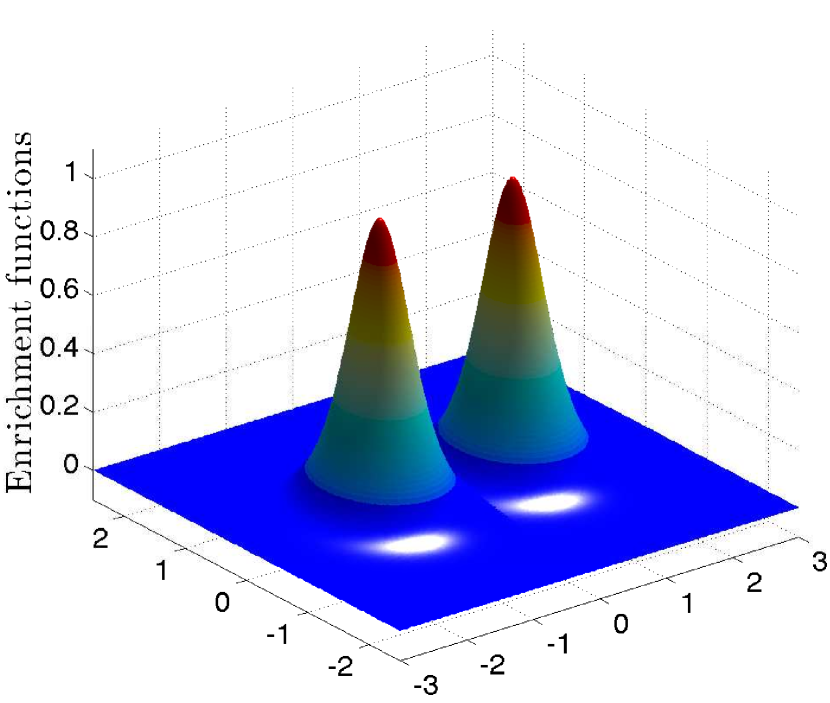
(a)

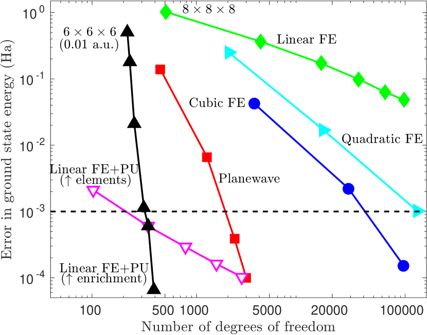
(b)

Figure 2: Localized (model pseudopotential) test problem. (a) Enrichment functions at $z=0$. (b) Error in computed ground state energy versus number of degrees of freedom using standard PW, real-space FE, and real-space PUFE methods. The coarsest mesh for linear FE is $8\times 8\times 8$. Linear FE + PU ($\uparrow$ enrichment) corresponds to linear FE with $6\times 6\times 6$ mesh and enrichment support radius increasing from $0.01$ a.u. to $2.51$ a.u. Linear FE + PU ($\uparrow$ elements) corresponds to linear FE with fixed enrichment support radius of $2.15$ a.u. and increasing number of elements in each direction.

6.2 Self-consistent calculations

Since the Fourier basis is global, the convergence of energies and eigenvalues with respect to number of basis functions (degrees of freedom) in the PW method is spectral, i.e., faster than any polynomial. In contrast, since finite element basis functions are polynomial in nature, the convergence of FE and other such real-space methods is determined by polynomial completeness. For a polynomial basis that is complete to order $p$, the errors in energies and eigenvalues of self-adjoint operators are $O(h^{2p})$, whereas the errors in the associated eigenfunctions are $O(h^{p+1})$ [25]. Hence, for sufficiently high accuracies, the spectral convergence of PW-based methods dominate and require fewer DOFs than fixed-degree polynomial based methods such as finite elements. However, at lower accuracies, with partition-of-unity enrichment in particular, the FE basis can require fewer DOFs, substantially fewer in fact, as we show below.

In the PUFE calculations that follow, we use cubic (serendipity) finite elements with 32 nodes per element, multiplied by appropriate phase factors at domain boundaries [58], to form the Bloch-periodic classical FE part $\{\phi_{i}(\bm{x})\}$ of the PUFE basis and trilinear finite elements with 8 nodes, multiplied by appropriate phase factors at domain boundaries, to form the Bloch-periodic partition of unity $\{\phi_{j}^{\textrm{PU}}(\bm{x})\}$. With both Bloch-periodic FE and Bloch-periodic partition of unity, the enrichment functions $\Psi_{\alpha}(\bm{x})$ are then constructed to be periodic [58], with $f(\mathbf{R})=1$ in (16).

6.2.1 LiH

We compare the PUFE method head-to-head against the current state-of-the-art PW method and standard FE method in total energy calculations of LiH, using hard, transferable HGH pseudopotentials [69]. The unit cell is cubic with lattice parameter $a=4.63$ bohr. The position of the Li atom in lattice coordinates is $\bm{\tau}=\bm{0}$ and that of the H atom is $\bm{\tau}=(1/2,1/2,1/2)$.

Two enrichments are used for Li (1s and 2s states in valence) and one enrichment for H (1s state in valence). The cutoff radius $r_{c}^{n\ell}$ for all enrichment functions is set to $2a$. Plots of the radial parts of the enrichment functions are shown in Fig. 3(a). The Brillouin zone is sampled at two $\bm{k}$-points: $\bm{k}=(0.00,\,0.00,\,0.00)$ and $\bm{k}=(0.12,\,-0.24,\,0.37)$. The reference result for the total energy is $-8.091160$ Ha, obtained from a PW calculation with 300 Ha planewave cutoff.

Figure 3(b) shows the error in computed total energy for LiH versus number of degrees of freedom (basis functions) using PW, real-space FE, and real-space PUFE methods. The horizontal line indicates an error of $10^{-3}$ Ha/atom, as typical in ab initio calculations. We first note that PW calculations require a factor of 9 fewer DOFs to reduce the error to the desired level than the real-space cubic FE method, which demonstrates the extent of the DOF disadvantage real-space methods must overcome to be competitive with planewaves. We now consider the cubic PUFE result. This achieves the required level of accuracy with a factor of 12 fewer DOFs than the PW method. The significant benefits of PU enrichment are manifest. On a fixed $3\times 3\times 3$ cubic FE mesh, increasing the enrichment support radii from 1.5 a.u. to 3.0 a.u. (just 64 additional DOFs) renders a more than two order of magnitude improvement in accuracy. Then, on refining the mesh for a fixed enrichment support radius of 3 a.u., the convergence rate of the PUFE error becomes comparable to standard cubic FE.

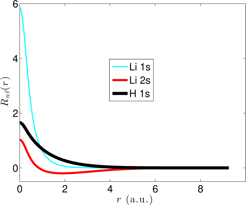
(a)

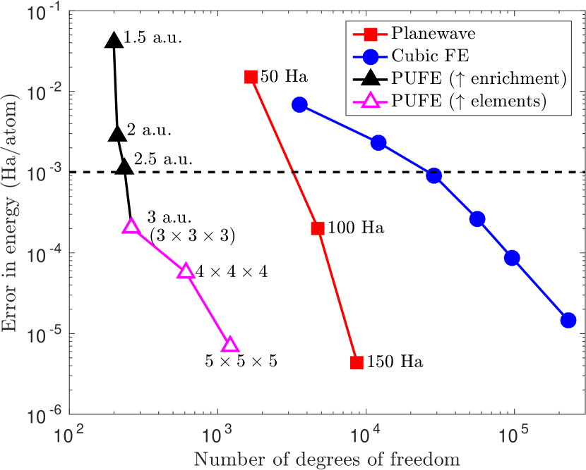
(b)

Figure 3: Enrichment functions and convergence of total energy for Kohn-Sham calculations of LiH. (a) Radial part of enrichment functions (1s and 2s for Li, 1s for H). (b) Error in computed total energy per atom of LiH versus number of degrees of freedom using standard PW, real-space FE, and real-space PUFE methods. Enrichment support radii and mesh sizes are indicated next to corresponding data points for PUFE. Planewave cutoffs are indicated next to corresponding data points for PW.

While increasing accuracy dramatically and retaining strict locality, the improvements afforded by partition-of-unity enrichment come with some cost: worsened conditioning. To quantify these aspects, we compute the sparsity and condition number of the overlap matrix in LiH calculations for a series of enrichment support radii. In Table 1, we report the sparsity and condition numbers of the overlap matrix for a $3\times 3\times 3$ cubic FE mesh and enrichment support radii $r_{e}=0,1,2,3$ a.u. ($r_{e}=0$ is a standard cubic FE calculation). For a fixed mesh spacing $h$, the condition number of the PUFE overlap matrix worsens with increasing enrichment support radius. Condition numbers in the range $10^{7}$ to $10^{9}$ in Table 1 are comparable to those of high-quality Gaussian basis sets in quantum chemistry [70]. The PUFE solution with $r_{e}=3$ delivers less than 1 mHa/atom error in energy (Fig. 3(b)). From Table 1, the sparsity of the overlap matrix is, however, just $38.3\,\%$. This is a consequence of the small 2-atom unit cell. Since the PUFE basis is strictly local, the number of nonzeros per row of the overlap matrix is independent of system size, and so sparsity increases with systems size. For example, for a 16-atom unit cell with $6\times 6\times 6$ cubic FE mesh and $r_{e}=3$, the sparsity of the overlap matrix increases to $92.1\,\%$. For small problems, where dense matrix methods can be applied, the conditioning presents no particular problem. However, for larger problems, where iterative methods must be employed, the conditioning requires special attention, as discussed in Ref. [71].

Table 1: Sparsity and condition number of PUFE overlap matrix for LiH calculation.

Method	$r_{e}$	Sparsity (%)	Condition number
FE	–	51.7	$2.2\times 10^{3}$
PUFE	1.0	51.2	$9.2\times 10^{6}$
PUFE	2.0	46.8	$1.3\times 10^{8}$
PUFE	3.0	38.3	$2.3\times 10^{9}$

6.2.2 CeAl

To assess the performance of the PUFE method in the worst case, we apply it to a difficult f-electron system: triclinic CeAl using hard, nonlocal HGH pseudopotentials [69], with atoms displaced from ideal positions. The unit cell is triclinic, with primitive lattice vectors and atomic positions

$$\bm{a}_{1} =a(1.00\quad 0.02\quad-0.04),$$

$$\bm{a}_{2} =a(0.01\quad 0.98\quad 0.03),$$ (17a)

$$\bm{a}_{3} =a(0.03\quad-0.06\quad 1.09),$$

$$\bm{\tau}_{\textrm{Ce}} =a(0.01\quad 0.02\quad 0.03),$$ (17b)

$$\bm{\tau}_{\textrm{Al}} =a(0.51\quad 0.47\quad 0.55),$$ (17c)

with lattice parameter $a=5.75$ bohr and atomic positions in lattice coordinates.

Because Ce has a full complement of s, p, d, and f states in valence, it requires 17 enrichment functions to span the occupied space (whereas, e.g., Li requires only two), making this a particularly severe test for the efficiency of PUFE relative to planewaves. The cutoff radius for all enrichment functions was 10 a.u. The radial parts of the enrichment functions for Ce and Al are shown in Figs. 4(a) and 4(b), respectively. The Brillouin zone is sampled at the same two $\bm{k}$-points used for LiH. The reference result for the total energy is $-40.675698$ Ha, taken from a planewave calculation with 170 Ha planewave cutoff. Figure 4(c) shows the error in the total energy for CeAl versus number of degrees of freedom using PW, real-space FE, and real-space PUFE methods. We first note that PW calculations require a factor of 16 fewer DOFs to reduce the error to the desired level than the real-space cubic FE method. We now consider the cubic PUFE result. Remarkably, even with the large number of enrichment functions for Ce, the PUFE method still attains the required accuracy with a factor of 5 fewer DOFs than the current state-of-the-art PW method.

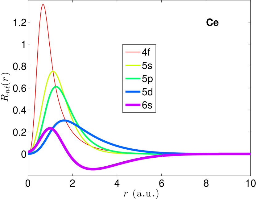
(a)

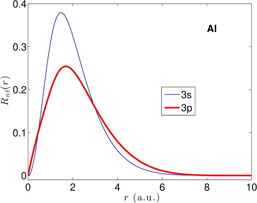
(b)

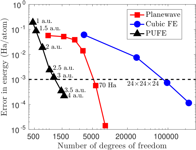
(c)

Figure 4: Enrichment functions and convergence of total energy for Kohn-Sham calculations of CeAl. Radial parts of enrichment functions for (a) Ce and (b) Al. (c) Convergence of computed total energy per atom for PW, real-space FE, and real-space PUFE methods versus number of degrees of freedom. PUFE calculations use a $4\times 4\times 4$ FE mesh. Enrichment support radii are indicated next to corresponding data points for PUFE. Planewave cutoff and FE mesh for $\sim 10^{-3}$ Ha/atom error are indicated next to corresponding points.

6.2.3 EOS of LiH

As a last example, we compute the equation of state (EOS) of LiH. The model of the unit cell for LiH and the enrichment functions for Li and H are shown in Fig. 3. The EOSs computed by PUFE, PW at 85 Ha cutoff, and PW at 200 Ha cutoff are shown in Fig. 5. The error for the PW calculation at 200 Ha cutoff is $\sim 10^{-6}$ Ha/atom, and so is taken as the reference. The PW calculation at 85 Ha cutoff required from 2398 basis functions at the smallest volume to 4132 basis functions at the largest volume to attain the required accuracy. In contrast, the PUFE calculation required just 269 basis functions to attain the required accuracy at all volumes, a more than order of magnitude reduction in total DOFs. The computed lattice constants and bulk moduli, obtained from a 4th order Birch-Murnaghan fit [72] are presented in Table 2. Both lattice constant and bulk modulus show excellent agreement with the PW benchmark, while obtained with a basis $\sim$ 1/40 the size.

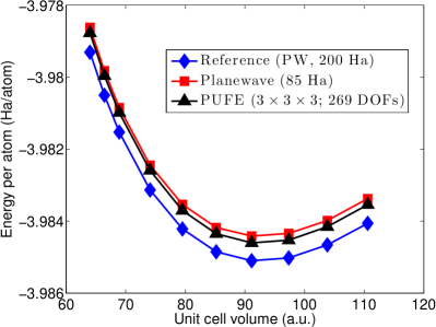
Figure 5: EOS of LiH computed by PW and PUFE methods.

Table 2: Equilibrium volume, lattice parameter, and bulk modulus of LiH computed by PW and PUFE methods.

Method	$V_{0}$ (Bohr3)	$a_{0}$ (Bohr)	$B_{0}$ (GPa)
PW (200 Ha)	92.5719	4.5237	45.6656
PW (85 Ha)	92.5885	4.5240	45.8108
PUFE	92.6241	4.5245	46.8282

7 Concluding remarks

In this paper, we have shown that a strictly local, systematically improvable, real-space basis can attain the accuracies required in quantum mechanical materials calculations with not only fewer but substantially fewer degrees of freedom than current state-of-the-art planewave based methods. This was achieved by building known atomic physics into the solution process using modern partition-of-unity techniques in finite element analysis. Our results show order-of-magnitude reductions in basis size relative to state-of-the-art PWs for a range of problems, especially those involving localized states. The method developed herein is completely general, applicable to any crystal symmetry and to both metals and insulators alike. The accuracy and rate of convergence were assessed on simple systems with light atoms (LiH) as well as a complex f-electron system (CeAl), which required a large number of atomic-orbital enrichments. In both cases, the PUFE method attained the required accuracies with 5 to 10 times fewer degrees of freedom than planewave-based methods. We computed the EOS of LiH and extracted its lattice constant and bulk modulus, finding again excellent agreement with benchmark planewave results, while requiring an order of magnitude fewer DOFs to obtain.

Having overcome the substantial degree-of-freedom disadvantage of real-space methods relative to current state-or-the-art PW methods, while retaining both strict locality and systematic improvability, there remain two key issues to be addressed: computational cost per degree of freedom and parallel implementation. First, to be competitive with existing parallel planewave codes in terms of time to solution will require an efficient parallel implementation which exploits the strict locality of the PUFE basis in real space and associated freedom from communication-intensive transforms such as FFTs. Second, to reduce computational cost per degree of freedom will require efficient solution of the sparse generalized eigenproblem generated by the method, which can become ill-conditioned. An algorithm for ill-conditioned generalized eigenproblems has been developed by Cai and coworkers [71] and has shown excellent efficiency when applied to PUFE system matrices but requires a sparse-direct factorization in its present formulation, limiting problem size. However, possibilities exist to avoid the ill-conditioned generalized eigenproblem as well. One such possibility is to employ flat-top partition-of-unity functions [73, 74], which can be constructed to mitigate ill-conditioning and deliver a standard, rather than generalized, eigenproblem. Another possibility is to move to a discontinuous representation [75], thus admitting any desired enrichment while retaining both orthonormality and strict locality. Both directions are being pursued by the authors presently.

8 Acknowledgments

This work was performed, in part, under the auspices of the U.S. Department of Energy by Lawrence Livermore National Laboratory under Contract DE-AC52-07NA27344. Support of the Laboratory Directed Research and Development program at the Lawrence Livermore National Laboratory is gratefully acknowledged. Additional financial support of the National Science Foundation through contract grant DMS-0811025 and the UC Lab Fees Research Program are also acknowledged. The authors are also grateful for the initial contributions of Murat Efe Guney, Wei Hu, and Seyed Ebrahim Mousavi in the implementation of the PUFE KS-DFT code.

Appendix A Supplementary Materials

A.1 Partition-of-unity finite-element method applied to a 1D model problem

To illustrate the substantial advantages of partition-of-unity enrichment in the context of problems where much is known about solutions locally, as in quantum mechanical calculations of molecular and condensed matter systems, we consider a 1D model problem. Let the one-dimensional domain $\Omega=[-\pi,\pi]$. We consider the approximation of a one-dimensional function $u(x):\Omega\rightarrow{\mathbb{R}}$ representative of a quantum-mechanical wavefunction in a molecule or solid (see Fig. 6):

$$u(x) =\Psi(x)+\delta(x),\quad x\in[-\pi,\pi]$$ (18a)

where

$$\Psi(x) =\exp(-ax^{2})\cos(bx),\quad x\in[-\pi,\pi],$$ (18b)

$$\delta(x) =c(1+dx^{2})\cos(x-0.5),\quad x\in[-\pi,\pi],$$ (18c)

and we choose $a=1.3$, $b=2.9$, $c=-0.15$, $d=0.25$.

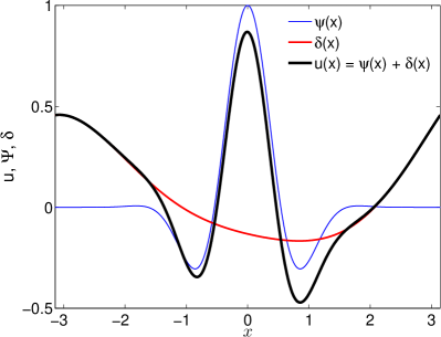
Figure 6: Model wavefunction $u(x)=\Psi(x)+\delta(x)$ in a solid, composed of isolated-atom like wavefunction $\Psi(x)$ and perturbation $\delta(x)$ due to interactions with neighboring atoms.

In (18c), $\delta(x)$ represents a perturbation arising from interactions with neighboring atoms. Let the domain be discretized by six elements as shown in Fig. 7(a). The coordinates of the seven nodes are: $x_{1}=-\pi$, $x_{2}=-2$, $x_{3}=-1$, $x_{4}=0$, $x_{5}=1$, $x_{6}=2$, $x_{7}=\pi$. Now, consider the following PUFE approximation:

$$u^{h}(x)=\sum_{i=1}^{7}\phi_{i}(x)u_{i}+\sum_{i=1}^{7}\phi_{i}(x)\Psi(x)b_{i}\equiv\sum_{j=1}^{14}\varphi_{j}(x)c_{j},$$

where $\phi_{i}(x)$ are linear finite element basis functions, $\Psi(x)$ is the enrichment function given in (18b), and the functions $\phi_{i}(x)$ serve as both standard FE basis and partition of unity for enrichment function $\Psi(x)$. If $b_{i}=0$ for all $i$, then we recover the standard FE approximation. To compute these coefficients for both FE and PUFE approximations, we construct the $L^{2}$ projection of $u(x)$ onto the space spanned by the PUFE basis $\{\varphi_{j}(x)\}$. Let

$$(u,w)\equiv(u,w)_{2}:=\int_{-\pi}^{\pi}uw\,dx$$

denote the $L^{2}$ inner product for functions $u,w\in L^{2}(-\pi,\pi)$. Then, the best-fit to $u(x)$ is obtained by minimizing $(u-u^{h},u-u^{h})/2$. Since

$$\tfrac{1}{2}(u-u^{h},u-u^{h})=\tfrac{1}{2}(u,u)-(u,u^{h})+\tfrac{1}{2}(u^{h},u^{h}),$$

we can equivalently minimize $\Pi(u,u^{h})=(u^{h},u^{h})/2-(u,u^{h})$. Now,

$$\tfrac{1}{2}(u^{h},u^{h}) =\tfrac{1}{2}\bm{c}^{T}\bm{M}\bm{c},\quad\bm{M}_{ij}=\int_{-\pi}^{\pi}\varphi_{i}(x)\varphi_{j}(x)\,dx,$$

$$(u,u^{h}) =\bm{c}^{T}\bm{f},\quad\bm{f}_{i}=\int_{-\pi}^{\pi}\varphi_{i}(x)u(x)\,dx,\quad\bm{c}=[c_{1}\dotsc c_{14}]^{T}.$$

Therefore, setting $\partial\Pi/\partial\bm{c}=\bm{0}$ leads to the following linear system of equations:

$$\bm{M}\bm{c}=\bm{f},$$ (19)

which is solved to obtain the minimizing coefficients $\bm{c}$.

The bases and resulting approximations are shown in Fig. 7. The classical FE basis functions $\phi_{i}(x)$ and PU enrichment functions $\phi_{i}(x)\Psi(x)$ are shown in Figs. 7(a) and 7(b), respectively. The PUFE basis then consists of the classical basis functions $\phi_{i}(x)$ and PU enrichment functions $\phi_{i}(x)\Psi(x)$ together. On comparing the FE and PUFE approximations shown in Figs. 7(c) and 7(d), the significant advantage of the PUFE basis is clear: the accuracy of the standard FE approximation is dramatically improved by adding the PU enrichment functions to the basis.

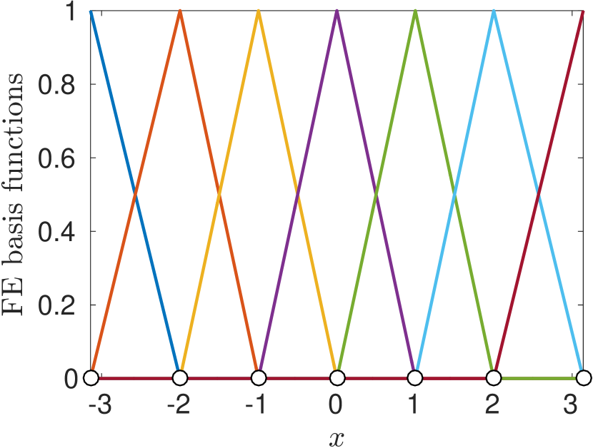
(a)

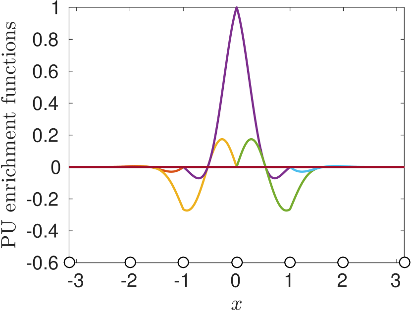
(b)

(c)

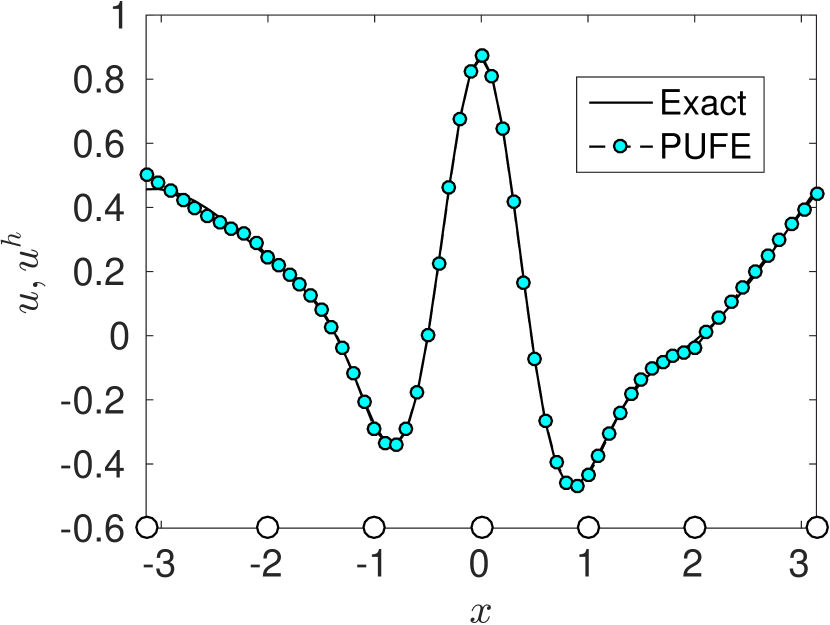
(d)

Figure 7: FE and PUFE approximations of model wavefunction. (a) FE basis functions. (b) PU enrichment functions. (c) FE approximation. (d) PUFE approximation.

References

- Hohenberg and Kohn [1964] P. Hohenberg and W. Kohn. Inhomogeneous electron gas. Phys. Rev., 136:B864–871, 1964.
- Kohn and Sham [1965] W. Kohn and L. J. Sham. Self-consistent equations including exchange and correlation effects. Phys. Rev., 140:A1133–1138, 1965.
- Pickett [1989] W. E. Pickett. Pseudopotential methods in condensed matter applications. Computer Phys. Rep., 9(3):115–197, 1989.
- Arias [1999] T. A. Arias. Multiresolution analysis of electronic structure: Semicardinal and wavelet bases. Rev. Mod. Phys., 71(1):267–311, 1999.
- Beck [2000] T. L. Beck. Real-space mesh techniques in density-functional theory. Rev. Mod. Phys., 72(4):1041–1080, 2000.
- Torsti et al. [2006] T. Torsti, T. Eirola, J. Enkovaara, T. Hakala, P. Havu, V. Havu, T. Höynälänmaa, J. Ignatius, M. Lyly, I. Makkonen, T. T. Rantala, J. Ruokolainen, K. Ruotsalainen, E. Räsänen, H. Saarikoski, and M. J. Puska. Three real-space discretization techniques in electronic structure calculations. Phys. Stat. Sol. (B), 243(5):1016–1053, 2006.
- Pask and Sterne [2005a] J. E. Pask and P. A. Sterne. Finite element methods in ab initio electronic structure calculations. Model. Simul. Mater. Sci. Eng., 13(3):R71–R96, 2005a.
- Genovese et al. [2008] L. Genovese, A. Neelov, S. Goedecker, T. Deutsch, S. A. Ghasemi, A. Willand, D. Caliste, O. Zilberberg, M. Rayson, A. Bergman, and R. Schneider. Daubechies wavelets as a basis set for density functional pseudopotential calculations. J. Chem. Phys., 129(1):014109, 2008.
- Saad et al. [2010] Y. Saad, J. R. Chelikowsky, and S. M. Shontz. Numerical methods for electronic structure calculations of materials. SIAM Rev., 52(1):3–54, 2010.
- Chelikowsky et al. [1994] J. R. Chelikowsky, N. Troullier, and Y. Saad. Finite-difference-pseudopotential method: Electronic-structure calculations without a basis. Phys. Rev. Lett., 72(8):1240–1243, 1994.
- Seitsonen et al. [1995] A. P. Seitsonen, M. J. Puska, and R. M. Nieminen. Real-space electronic-structure calculations: Combination of the finite-difference and conjugate-gradient methods. Phys. Rev. B, 51(20):14057–14061, 1995.
- Gygi and Galli [1995] F. Gygi and G. Galli. Real-space adaptive-coordinate electronic-structure calculations. Phys. Rev. B, 52(4):R2229–R2232, 1995.
- Iyer et al. [1995] K. A. Iyer, M. P. Merrick, and T. L. Beck. Application of a distributed nucleus approximation in grid based minimization of the Kohn-Sham energy functional. J. Chem. Phys., 103(1):227–233, 1995.
- Hoshi et al. [1995] T. Hoshi, M. Arai, and T. Fujiwara. Density-functional molecular-dynamics with real-space finite-difference. Phys. Rev. B, 52(8):R5459–R5462, 1995.
- Briggs et al. [1996] E. L. Briggs, D. J. Sullivan, and J. Bernholc. Real-space multigrid-based approach to large-scale electronic structure calculations. Phys. Rev. B, 54(20):14362–14375, 1996.
- Modine et al. [1997] N. A. Modine, G. Zumbach, and E. Kaxiras. Adaptive-coordinate real-space electronic-structure calculations for atoms, molecules, and solids. Phys. Rev. B, 55(16):10289–10301, 1997.
- Fattebert [1999] J.-L. Fattebert. Finite difference schemes and block Rayleigh Quotient Iteration for electronic structure calculations on composite grids. J. Comp. Phys., 149(1):75–94, 1999.
- Fattebert and Bernholc [2000] J.-L. Fattebert and J. Bernholc. Towards grid-based O(N) density-functional theory methods: optimized non-orthogonal orbitals and multigrid acceleration. Phys. Rev. B, 62(3):1713–1722, 2000.
- Fattebert and Gygi [2004] J.-L. Fattebert and F. Gygi. Linear scaling first-principles molecular dynamics with controlled accuracy. Comput. Phys. Comm., 162:24–36, 2004.
- Alemany et al. [2004] M. M. G. Alemany, M. Jain, L. Kronik, and J. R. Chelikowsky. Real-space pseudopotential method for computing the electronic properties of periodic systems. Phys. Rev. B, 69(7):075101, 2004.
- Beck [2009] T. L. Beck. Real-space and multigrid methods in computational chemistry. In K. B. Lipkowitz and T. R. Cundari, editors, Reviews in Computational Chemistry, volume 26, pages 223–285. 2009.
- Ghosh and Suryanarayana [2016a] S. Ghosh and P. Suryanarayana. SPARC: Accurate and efficient finite-difference formulation and parallel implementation of density functional theory: Isolated clusters. arXiv preprint arXiv:1603.04334, 2016a.
- Ghosh and Suryanarayana [2016b] S. Ghosh and P. Suryanarayana. SPARC: Accurate and efficient finite-difference formulation and parallel implementation of density functional theory: Extended systems. arXiv preprint arXiv:1603.04339, 2016b.
- Ono and Hirose [1999] T. Ono and K. Hirose. Timesaving double-grid method for real-space electronic-structure calculations. Phys. Rev. Lett., 82(25):5016–5019, 1999.
- Strang and Fix [1973] G. Strang and G. J. Fix. An Analysis of the Finite Element Method. Prentice-Hall, Englewood Cliffs, 1973.
- Askar [1975] A. Askar. Finite-element method for bound-state calculations in quantum-mechanics. J. Chem. Phys., 62(2):732–734, 1975.
- White et al. [1989] S. R. White, J. W. Wilkins, and M. P. Teter. Finite-element method for electronic-structure. Phys. Rev. B, 39(9):5819–5833, 1989.
- Hermansson and Yevick [1986] B. Hermansson and D. Yevick. Finite-element approach to band-structure analysis. Phys. Rev. B, 33(10):7241–7242, 1986.
- Tsuchida and Tsukada [1995] E. Tsuchida and M. Tsukada. Electronic-structure calculations based on the finite-element method. Phys. Rev. B, 52(8):5573–5578, 1995.
- Tsuchida and Tsukada [1998] E. Tsuchida and M. Tsukada. Large-scale electronic-structure calculations based on the adaptive finite-element method. J. Phys. Soc. Jpn., 67(11):3844–3858, 1998.
- Tsuchida and Tsukada [1996] E. Tsuchida and M. Tsukada. Adaptive finite-element method for electronic-structure calculations. Phys. Rev. B, 54(11):7602–7605, 1996.
- Pask et al. [1999] J. E. Pask, B. M. Klein, C. Y. Fong, and P. A. Sterne. Real-space local polynomial basis for solid-state electronic-structure calculations: A finite-element approach. Phys. Rev. B, 59(19):12352–12358, 1999.
- Pask et al. [2001] J. E. Pask, B. M. Klein, P. A. Sterne, and C. Y. Fong. Finite-element methods in electronic-structure theory. Comput. Phys. Commun., 135(1):1–34, 2001.
- Pask and Sterne [2005b] J. E. Pask and P. A. Sterne. Real-space formulation of the electrostatic potential and total energy of solids. Phys. Rev. B, 71(11):113101, 2005b.
- Motamarri et al. [2013] P. Motamarri, M. Nowak, K. Leiter, J. Knap, and V. Gavini. Higher-order adaptive finite-element methods for Kohn-Sham density functional theory. J. Comp. Phys., 253:308–343, 2013.
- Tsuchida et al. [2015] E. Tsuchida, Y.-K. Choe, and T. Ohkubo. Adaptive finite-element method for large-scale ab initio molecular dynamics simulations. Phys. Chem. Chem. Phys., 17(47):31444–31452, 2015.
- Batcho [2000] P. F. Batcho. Computational method for general multicenter electronic structure calculations. Phys. Rev. E, 61(6, Part B):7169–7183, 2000.
- Lehtovaara et al. [2009] L. Lehtovaara, V. Havu, and M. Puska. All-electron density functional theory and time-dependent density functional theory with high-order finite elements. J. Chem. Phys., 131(5):054103, 2009.
- Zhang et al. [2008] D. Zhang, L. H. Shen, A. H. Zhou, and X. G. Gong. Finite element method for solving Kohn-Sham equations based on self-adaptive tetrahedral mesh. Phys. Lett. A, 372:5071–5076, 2008.
- Bylaska et al. [2009] E. J. Bylaska, M. Holst, and J. H. Weare. Adaptive finite element method for solving the exact Kohn-Sham equation of density functional theory. J. Chem. Theory Comput., 5(4):937–948, 2009.
- Alizadegan et al. [2010] R. Alizadegan, K. J. Hsia, and T. J. Martínez. A divide and conquer real space finite-element Hartree-Fock method. J. Chem. Phys., 132:034101, 2010.
- Bao et al. [2012] G. Bao, G. Hu, and D. Liu. An -adaptive finite element solver for the calculations of the electronic structures. J. Comp. Phys., 231(14):4967–4979, 2012.
- Schauer and Linder [2013] V. Schauer and C. Linder. All-electron Kohn-Sham density functional theory on hierarchic finite element spaces. J. Comp. Phys., 250:644–664, 2013.
- Schauer and Linder [2015] V. Schauer and C. Linder. The reduced basis method in all-electron calculations with finite elements. Adv. Comput. Math., 41(5):1035–1047, 2015.
- Motamarri and Gavini [2014] P. Motamarri and V. Gavini. A subquadratic-scaling subspace projection method for large-scale Kohn-Sham DFT calculations using spectral finite-element discretization. Phys. Rev. B, 90:115127, 2014.
- Chen et al. [2014] H. Chen, X. Dai, X. Gong, L. He, and A. Zhou. Adaptive finite element approximations for Kohn-Sham models. Multiscale Model. Sim., 12(4):1828–1869, 2014.
- Maday [2014] Y. Maday. – finite element approximation for full-potential electronic structure calculations. Chinese Ann. Math. B, 35(1):1–24, 2014.
- Davydov et al. [2016] D. Davydov, T. D. Young, and P. Steinmann. On the adaptive finite element analysis of the Kohn-Sham equations: methods, algorithms, and implementation. Internat. J. Numer. Methods Engrg., 106:863–888, 2016.
- Skriver [1984] H. L. Skriver. The LMTO Method. Springer, Berlin, 1984.
- Singh and Nordstrom [2006] D. J. Singh and L. Nordstrom. Planewaves, Pseudopotentials, and the LAPW Method. Springer, New York, 2nd edition, 2006.
- Boys [1950] S. F. Boys. Electronic wave functions. I. A general method of calculation for the stationary states of any molecular system. Proc. R. Soc. Lon. A, 200(1063):542–554, 1950.
- Dusterhoft et al. [1998] C. Dusterhoft, D. Heinemann, and D. Kolb. Dirac-Fock-Slater calculations for diatomic molecules with a finite element defect correction method (FEM-DKM). Chem. Phys. Lett., 296(1-2):77–83, 1998.
- Yamakawa and Hyodo [2003] S. Yamakawa and S. Hyodo. Electronic state calculation of hydrogen in metal clusters based on Gaussian-FEM mixed basis function. J. Alloy. Compd., 356(2):231–235, 2003.
- Yamakawa and Hyodo [2005] S. Yamakawa and S. Hyodo. Gaussian finite-element mixed-basis method for electronic structure calculations. Phys. Rev. B, 71(3):035113, 2005.
- Jun [2004] S. Jun. Meshfree implementation for the real-space electronic-structure calculation of crystalline solids. Internat. J. Numer. Methods Engrg., 59(14):1909–1923, 2004.
- Chen et al. [2007] J. S. Chen, H. Wu, and M. A. Puso. Orbital HP-cloud for solving Schrödinger equation in quantum mechanics. Comput. Methods Appl. Mech. Engrg., 196(37–40):3693–3705, 2007.
- Suryanarayana et al. [2011] P. Suryanarayana, K. Bhattacharya, and M. Ortiz. A mesh-free convex approximation scheme for Kohn-Sham density functional theory. J. Comp. Phys., 230:5226–5238, 2011.
- Sukumar and Pask [2009] N. Sukumar and J. E. Pask. Classical and enriched finite element formulations for Bloch-periodic boundary conditions. Internat. J. Numer. Methods Engrg., 77(8):1121–1138, 2009.
- Pask et al. [2012] J. E. Pask, N. Sukumar, and S. E. Mousavi. Linear scaling solution of the all-electron Coulomb problem in solids. Int. J. Multiscale Comp. Eng., 10(1):83–99, 2012.
- Pask et al. [2011] J. E. Pask, N. Sukumar, M. Guney, and W. Hu. Partition-of-unity finite-element method for large scale quantum molecular dynamics on massively parallel computational platforms. Technical Report LLNL-TR-470692, Department of Energy LDRD Grant 08-ERD-052, March 2011.
- Melenk and Babuška [1996] J. M. Melenk and I. Babuška. The partition of unity finite element method: Basic theory and applications. Comput. Methods Appl. Mech. Engrg., 139:289–314, 1996.
- Babuška and Melenk [1997] I. Babuška and J. M. Melenk. The partition of unity method. Internat. J. Numer. Methods Engrg., 40:727–758, 1997.
- Perdew et al. [1996] J. P. Perdew, K. Burke, and M. Ernzerhof. Generalized gradient approximation made simple. Phys. Rev. Lett., 18:3865, 1996.
- Martin [2004] R. M. Martin. Electronic Structure: Basic Theory and Practical Methods. Cambridge University Press, Cambridge, 2004.
- Ashcroft and Mermin [1976] N. W. Ashcroft and N. D. Mermin. Solid State Physics. Holt, Rinehart and Winston, New York, 1976.
- Griffiths [1994] D. J. Griffiths. Introduction to Quantum Mechanics. Prentice Hall, Englewood Cliffs, 1994.
- Mousavi et al. [2012] S. E. Mousavi, J. E. Pask, and N. Sukumar. Efficient adaptive integration of functions with sharp gradients and cusps in -dimensional parallelepipeds. Internat. J. Numer. Methods Engrg., 91(4):343–357, 2012.
- Gygi [1992] F. Gygi. Adaptive Riemannian metric for plane-wave electronic-structure calculations. Europhys. Lett., 19(7):617–622, 1992.
- Hartwigsen et al. [1998] C. Hartwigsen, S. Goedecker, and J. Hutter. Relativistic separable dual-space Gaussian pseudopotentials from H to Rn. Phys. Rev. B, 58(7):3641–3662, 1998.
- Rappoport and Furche [2010] D. Rappoport and F. Furche. Property-optimized gaussian basis sets for molecular response calculations. J. Chem. Phys., 133:134105, 2010.
- Cai et al. [2013] Y. Cai, Z. Bai, J. E. Pask, and N. Sukumar. Hybrid preconditioning for iterative diagonalization of ill-conditioned generalized eigenvalue problems in electronic structure calculations. J. Comp. Phys., 255:16–30, 2013.
- Birch [1947] F. Birch. Finite elastic strain of cubic crystals. Phys. Rev., 71(11):809, 1947.
- Schweitzer [2011] M. A. Schweitzer. Stable enrichment and local preconditioning in the particle-partition of unity method. Numer. Math., 118:137–170, 2011.
- Schweitzer [2013] M. A. Schweitzer. Variational mass lumping in the partition of unity method. SIAM J. Sci. Comput., 35(2):A1073–A1097, 2013.
- Lin et al. [2012] L. Lin, J. Lu, L. Ying, and W. E. Adaptive local basis set for Kohn-Sham density functional theory in a discontinuous Galerkin framework I: Total energy calculation. J. Comp. Phys., 231(4):2140–2154, 2012.