Inter-WBANs Interference Mitigation Using Orthogonal Walsh Hadamard Codes

Abstract

A Wireless Body Area Network (WBAN) provides health care services. The performance and utility of WBANs can be degraded due to interference. In this paper, our contribution for co-channel interference mitigation among coexisting WBANs is threefold. First, we propose a distributed orthogonal code allocation scheme, namely, OCAIM, where, each WBAN generates sensor interference lists (SILs), and then all sensors belonging to these lists are allocated orthogonal codes. Secondly, we propose a distributed time reference correlation scheme, namely, DTRC, that is used as a building block of OCAIM. DTRC enables each WBAN to generate a virtual time-based pattern to relate the different superframes. Accordingly, DTRC provides each WBAN with the knowledge about, 1) which superframes and, 2) which time-slots of those superframes interfere with the time-slots within its superframe. Thirdly, we further analyze the success and collision probabilities of frames transmissions when the number of coexisting WBANs grows. The simulation results demonstrate that OCAIM outperforms other competing schemes in terms of interference mitigation and power savings.

I Introduction

A WBAN is a wireless emerging technology consisting of a coordinator and multiple low power, wearable or implanted tiny sensors for collecting health related data about the physiological state of human body. WBANs are used in many applications such as medical treatment and diagnosis, consumer electronics, sports and military [7]. For example, these sensors may observe the heart and the brain electrical activities as well as vital signs and parameters like insulin percentage in blood, blood pressure, temperature, etc.

Recently, the IEEE 802.15.4 standard has proposed new protocols for WBANs and specified an upper limit for the number of WBANs (60 sensors in $6m^{3}$ and 256 sensors in $3m^{3}$ space) that properly coexist [14]. The standard proposes three mechanisms for co-channel interference mitigation, namely, beacon shifting, channel hopping and active superframe interleaving. Nevertheless, there is a great possibility of co-channel interference among coexisting WBANs, e.g., inside hospital’s corridor crowded with patients. Hence, communication links may suffer interference, and consequently the performance and quality of service requirements of each individual WBAN may quickly degrade. Therefore, interference mitigation is quite necessary for reliable communication in WBANs.

In addition, the highly mobile and resource constrained nature of WBANs make co-channel interference mitigation quite challenging. Such nature makes the allocation of global coordinator to manage multiple WBANs coexistence as well as the application of advanced antenna and power control techniques used in cellular networks unsuitable for WBANs. Moreover, due to the absence of coordination and synchronization among WBANs, the superframes of different nearby WBANs may overlap, and hence, their concurrent transmissions may interfere. More specifically, when two or more sensors of different WBANs access the shared channel at the same time and therefore, the co-channel interference may arise. In this paper, we tackle these issues and contribute the following:

• DTRC, a scheme for determining which superframes and their corresponding times slots overlap with each others

• OCAIM, a scheme that allocates orthogonal codes to interfering sensors belonging to sensor interference lists

• An analysis of the success and collision probability model for frames transmissions

Simulation results and theoretical analysis show that our proposed approach can significantly increase the minimum signal to interference plus noise ratio (SINR) and the energy savings of each WBAN. Additionally, our proposed scheme significantly diminishes the inter-WBAN interference level and adds no complexity to the sensors as the coordinators are only required to compute and negotiate for orthogonal code assignment.

The rest of the paper is organized as follows. Section ii@ discusses the related work. Section iii@ states the system model and covers some preliminaries. Section iv@ explains our distributed time reference correlation scheme. Section v@ describes our proposed interference mitigation scheme using orthogonal codes. Section vi@ mathematically analyzes the performance of OCAIM. Section vii@ presents the simulation results. Finally, the paper is concluded in Section viii@.

II Related Work

Prior work has addressed the problem of co-channel interference in WBANs through spectrum allocation, cooperation, power control, game theory and multiple access schemes. Examples of spectrum allocation techniques include [10, 8, 13, 9]. However, in [9], a prediction algorithm for dynamic channel allocation is proposed where, variations of channel assignment due to WBANs mobility are investigated. In [8], a dynamic resource allocation is proposed where, orthogonal channels are allocated for interfering sensors belonging to each pair of WBANs. Movassaghi et al., [13] have proposed an adaptive interference avoidance scheme that considers sensor-level interference only. Further, the proposed scheme allocates synchronous and parallel transmission intervals and significantly reduces the number of assigned channels. Whereas, our approach considers both sensor- and time-slot-level interference and significantly diminishes the latter as well as better improves the power savings of WBANs. Whilst, Liang et al., [10] have analyzed the inter-WBAN interference using various performance metrics and then, proposed interference detection and mitigation scheme using dynamic channel hopping.

Meanwhile, other approaches have adopted cooperative communication, game theory and power control to mitigate co-channel interference. Dong et al., [5] have pursued joint cooperative and power control communication for WBANs coexistence problem. Similarly, in [2], intra-WBAN interference is mitigated using cooperative orthogonal channels and a contention window extension mechanism. Whereas, the approach of [12] employs a Bayesian game based power control to mitigate inter-WBAN interference by modeling WBANs as players and active links as types of players in the Bayesian model. Other approaches pursued multiple access schemes for interference mitigation. In [4], multiple WBANs collaborate to agree on common TDMA schedule that avoids the co-channel interference. Whilst, Kim et al., [6] have proposed distributed TDMA-based beacon interval shifting scheme for interference mitigation where, the wakeup period of each WBAN coinciding with other WBANs is avoided by employing carrier sense before a beacon transmission. Also, Chen et al., [1] adopts TDMA for scheduling transmissions within a WBAN and carrier sensing mechanism to deal with inter-WBAN interference.

In this paper, we take a step forward and consider the sensor- and time-slot- levels interference mitigation amongst coexisting WBANs. More specifically, we allocate orthogonal code to each interfering sensor in its assigned time-slot to avoid interference with other WBANs’ sensors. Meanwhile, we depend on distributed time reference correlation and time provisioning to determine which superframes overlap with each other.

III System Model and Preliminaries

III-A Model Description and Assumptions

Let us consider a network composed of N coexisting TDMA-based WBANs, each consists of up to K sensors that transmit their data to a single coordinator denoted by C. All sensors transmit at maximum data rate of 250Kb/s within the 2.4 GHz unlicensed international band using the same transmission power (-10 dBm), modulation scheme and average transmitted energy per symbol. Furthermore, we assume that the superframes of different WBANs are neither aligned nor synchronized and may overlap with each other.

III-B Interference Lists (I)

Let us assume when $k^{th}$ sensor $S_{i,k}$ of $WBAN_{i}$ is transmitting to its $C_{i}$, in the same time, all other coordinators compute the power received from $S_{i,k}$’s transmitted signal. Let $\delta_{i,j,k}$ denotes the power received from the $k^{th}$ sensor of $WBAN_{j}$ at the coordinator of $WBAN_{i}$. After all transmissions are over in the first round, each $C_{i}$ creates a table consisting of power received from all sensors in the network. Furthermore, we denote the minimum power received within a $WBAN_{i}$ by $\rho_{i}^{min}=min\{\delta_{i,k=1,\dots,K}\}$. Therefore, we denote the interference list of $WBAN_{i}$ by $I_{i}$ and defined as in eq. (1) below.

$$I_{i}=\{S_{l,m}|\delta_{i,l,m}>\rho_{i}^{min}-\theta,\forall i\neq l\}$$ (1)

Where $\theta$ is the interference threshold, afterwards, each $C_{i}$ broadcasts $I_{i}$ to all network coordinators.

III-C Interference Sets (IS)

Based on power tables update (using the broadcast among WBANs), each $C_{i}$ verifies which of its sensors impose interference on sensors of other WBANs and which sensors of other WBANs impose interference on its WBAN’s sensors. It then creates an interference set denoted by $IS_{i}$ and defined as in eq. (2) below.

$$IS_{i}=I_{i}\cup\{S_{i,k}|S_{i,k}\in I_{l},\forall l\neq i\}$$ (2)

III-D Cyclic Orthogonal Walsh Hadamard Codes (COWHC)

In this section, we provide a brief overview of cyclic orthogonal Walsh Hadamard codes that we used in our interference mitigation approach [3]. The network consisting of N coexisting WBANs that communicate over shared channel where each coordinator is assigned a unique orthogonal spreading code for its WBAN. In a time-slot $TS_{i}$ of sensor $r_{i}$ of a $WBAN_{i}$, $r_{i}$ multiplies its modulated signal $s_{i}$ by the spreading code $\omega_{i}$. We assume the worst case scenario when $r_{i}$ is interfering with N-1 sensors in $TS_{i}$. The received signal $X_{r}$ at coordinator $C_{i}$ of $WBAN_{i}$ is given by eq. (3) below.

$$X_{r}=\omega_{i}\cdot s_{i}+{\sum_{j=1,j\neq i}^{N-1}\omega_{j}\cdot s_{j}+\mu}$$ (3)

Inherently the codes generated from the Walsh Hadamard denoted by WH matrix $M_{2^{n}}$ are orthogonal in the zero-phase with N = n + 1. $M_{2^{n}}$ is a special matrix of size $2^{N}$ $\times$ $2^{N}$.

$$M_{1}=\begin{pmatrix}1\end{pmatrix},M_{2}=\begin{pmatrix}1&1\\ 1&-1\end{pmatrix}$$ (4)

are given, one can generate a generic WH matrix $M_{2^{n}}$, $n>1$, as follows.

$$M_{2^{n}}=\begin{pmatrix}M_{2^{n}-1}&M_{2^{n}-1}\\ M_{2^{n}-1}&M_{2^{n}-1}\end{pmatrix}=M_{2}\otimes M_{2^{n}-1}$$ (5)

Where $\otimes$ denotes the Kronecker product. The rows in each matrix generated in eq. (5) are orthogonal to each other. However, the orthogonality property of WH codes is lost if the codes are phase shifted. So, a special set of codes extracted from the WH matrix $M_{2^{k}}$ is required to keep orthogonality property with any phase shift ($\phi=0,1,2,\dots 2^{k}-1$). Thus, one can extract N = n + 1 orthogonal codes from $M_{2^{k}}$ matrix that have zero cross correlation for all $\phi=0,1,2,\dots 2^{k}-1$. This set of N cyclic orthogonal spreading codes is called Orthogonal Walsh Hadamard Codes and denoted by (COWHC). If the COWHC set is used for spreading in the network, then, $d_{i}$ is the decoded signal of high interfering sensor $r_{i}$ at $C_{i}$, where,

$$d_{i}=\omega_{i}\cdot X_{r}=\omega_{i}^{2}\cdot s_{i}+\sum_{j=1,j\neq i}^{N-1}\omega_{i}\cdot\omega_{j}\cdot s_{j}+\omega_{i}\cdot\mu$$ (6)

$\omega_{i}^{2}$ = 1 and $\omega_{i}\cdot\omega_{j}=0$ due to their orthogonality. Therefore, the decoded signal is $d_{i}$ = $s_{i}$ + $\omega_{i}\cdot\mu$.

IV A Distributed Time Reference Correlation Scheme (DTRC)

A WBAN’s superframe is delimited by two beacons and composed of equal length active and inactive periods that are dedicated for the sensors and the coordinators, respectively, as shown in Figure 1.

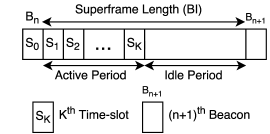
Figure 1: Superframe structure proposed for OCAIM scheme

Due to the absence of inter-WBAN coordination and central unit to manage coexistence amongst WBANs, hence, each WBAN’s transmission may face collisions with other WBANs’ transmissions in the same time-slots. In this work, we do not aim to interleave the superframes or add extra time intervals to avoid collisions. Instead, we present a distributed approach, namely, DTRC to avoid such collisions and minimize the time delay of each sensor’s transmission. DTRC allows each WBAN to relate the start time of other superframes to its local time and hence to predict which sensors within its WBAN will be interfering with sensors of other WBANs. Thus, all coordinators generate virtual time-based patterns involving the schedule of the transmission and reception of frames. More precisely, each coordinator according to its local clock calculates the timeshift from the actual start transmission time of a frame. Basically, the timeshift comprises, 1) non-deterministic parameters such as the synchronization error tolerance, the timing uncertainty and the clock drift and, 2) the difference between the non-deterministic parameters and the virtual start transmission time of a frame [14]. We define the following parameters that we used in our proposed DTRC scheme:

• PHY Timestamp (PTP), encodes the time when the last bit of the frame has transmitted to the air

• MAC Timestamp (MTP), encodes the time when the last bit of a frame has been transmitted at the MAC

• PHY Receiving Time (PRT), a time elapsed from the first to the last bit of a frame at the PHY

• MAC Receiving Time (MRT), a time elapsed from receiving the first bit to the last bit of a frame at the MAC

• Propagation Delay (L), a time elapsed by the bit to travel from the transmitter to the receiver through the air

• PHY Processing Time (PPT), a time elapsed from receiving the last bit of a frame at PHY until the delivery of the first bit to the MAC

• Frame Reception time (FRT), encodes the time when the last bit of a frame has been received at the MAC

Whenever a coordinator has a frame to transmit, the MAC service (resp. the PHY service) adds a MAC-level timestamp denoted by MTP (resp. PHY-level timestamp denoted by PTP) that encodes the time when the last bit of the frame is transmitted to the PHY layer (resp. to the air). Such addition with other PHY- and MAC-level parameters enable the receiving coordinator to calculate the timeshift. Furthermore, when the coordinator receives a frame at the MAC, it timestamps the reception of the last bit of that frame through FRT according to its local clock. Thus, as the frame bits pass through the PHY and MAC layers, the receiving services at each layer calculates the following parameters: 1) the time spent by the MAC service to receive the frame (MRT), 2) the time spent by the PHY service to process the frame (PPT), 3) the time spent by the PHY service to receive the frame (PRT) and, 4) the time spent by the first bit of the frame to be received at the PHY from the air.

Subsequently, each coordinator relates the calculated parameters and timestamps as well as the frame reception times to compute the timeshift as shown in Algorithm 1. Afterwards, it generates a pattern which consists of the different computed timeshifts of the different superframes. Based on a timeshift of a particular superframe, the coordinator aligns the start transmission time of its superframe to the superframe of that timeshift to predict which time-slots within its superframe are interfering with the time-slots of that superframe. To summarize, DTRC provides each coordinator with two fundamental functionalities, 1) it determines which superframes may overlap, and more precisely, 2) which time-slots within those superframes may collide with each other as shown in Figure 2. The pseudocode of DTRC is described in Algorithm 1.

input :

N WBANs, K Sensors/WBAN, K Slots/Superframe

for i $\leftarrow$ 1 to N do

2      for l $\leftarrow$ 1 to $N-1$ $\&$ i $\neq$ l do

3            $C_{i}$ receives $B^{l}$ at $FRT_{i,l}$ $\&$ $C_{i}$ computes: $Diff_{l}=PTP_{l}-MTP_{l}=PPT_{l}+PRT_{l}$ $timehift_{i,l}=FRT_{i}-[MRT_{i}+PPT_{i}+PRT_{i}+L+Diff_{l}]$ $IntrfrnSlots_{i,l}=timehift_{i,l}/TS$ $ID$ = $\lceil\>\mid IntrfrnSlots_{i,l}\mid\>\rceil$ switch ($timehift_{i,l}$) case ’$timeshift_{i,l}$ $<$ $0$ $\&$ ($\mid timeshift_{i,l}\mid$ $<$ $TS$)’:        ($\forall$ $z$ $\geq$ $ID$ $\&$ $\forall$ $t$ $\geq$ $ID$), $T_{i,z}$ $\bowtie$ $T_{l,t}$ case ’$timeshift_{i,l}$ $<$ $0$ $\&$ ($TS$ $<$ $\mid$ $timeshift_{i,l}$ $\mid$ $<$ $BI/2$)’:        ($\forall$ $z$ $>$ $(K-ID)$ $\&$ $\forall$ $t$ $\leq$ $ID$), $T_{i,z}$ $\bowtie$ $T_{l,t}$ case ’$timeshift_{i,l}$ = $0$’:        Complete interference of $C_{l}$ $\&$ $C_{i}$ active periods

4       end for

5      

6 end for

Algorithm 1 Proposed DTRC Scheme

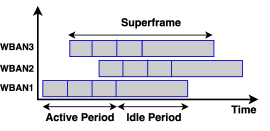
Figure 2: Overlapping superframes scheme

V Interference Mitigation Using Distributed Orthogonal Codes (OCAIM)

As aforementioned, when two or more sensors of different coexisting WBANs in the same area simultaneously access the shared channel as shown in Figure 3, a co-channel interference may arise. Hence, the superframes of different WBANs may overlap as shown in Figure 2. In our proposed OCAIM scheme, each WBAN is allocated a unique cyclic orthogonal code from the set COWHC. However, based on the interference that a particular sensor suffers in one or more time-slots it has been assigned, the coordinator commands that sensor to use the code in that time-slots for spreading its signal. Doing so, each sensor multiplies its signal by a spreading code to increase the bandwidth of that signal and then to become anti-interference. Furthermore, each coordinator updates its code assignment pattern with every new superframe. Additionally, it is important to note that spread spectrum techniques use the same transmit power levels because they transmit at a much lower spectral power density than that of the narrow band transmitters [14].

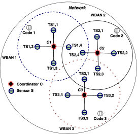
Figure 3: A network of three coexisting WBANs

We denote $k^{th}$ Sensor Interference List of sensor $S_{i,k}$ of $WBAN_{i}$ by $SIL_{i,k}$ that comprises all sensors of other WBANs which impose interference on $S_{i,k}$. Hence, $C_{i}$ adds all sensors $S_{l,m}$ to $SIL_{i,k}$ that, 1) interfere with $S_{i,k}$ in its assigned time-slot $T_{i,k}$ denoted by $S_{l,m}\bowtie S_{i,k}$ (time-slot level interference is determined by DTRC) and, 2) whose binary bitwise OR with that of $S_{i,k}$ equals to 1 denoted by $F_{i,k}$ $\otimes F_{l,m}=1$, where $F_{i,k}$ and $F_{l,m}$ are indicator functions respectively defined as follows.

$$F_{i,k}=\begin{cases}1&\quad if\;S_{i,k}\in IN_{i,l}\\ 0&\quad if\;S_{i,k}\notin IN_{i,l}\\ \end{cases}$$

,

$$F_{l,m}=\begin{cases}1&\quad if\;S_{l,m}\in IN_{i,l}\\ 0&\quad if\;S_{l,m}\notin IN_{i,l}\\ \end{cases}$$

I.e., $WBAN_{l}$ is an interferer to $WBAN_{i}$ and $IN_{i,l}=IS_{i}\cap IS_{l}$. Then, we define $SIL_{i}$ as in eq. (7) below.

$$SIL_{i,k}=\{S_{l,m}|T_{l,m}\bowtie T_{i,k}\>\&\>F_{i,k}\otimes F_{l,m}=1\}$$ (7)

Therefore, $C_{i}$ assigns a code to $S_{i,k}$ within its WBAN and each sensor belongs to $SIL_{i,k}$ is also assigned a code within its WBAN to avoid the interference. In other words, all interfering sensors of the same WBAN use the same code, each in its assigned time-slot since TDMA is used within each WBAN.

We illustrate our approach through an example of three coexisting TDMA-based WBANs scenario as shown in Figure 3. However, we denote $j^{th}$ sensor of $\textit{WBAN}_{i}$ is transmitting to its coordinator $C_{i}$ by $S_{i,j}$. Assuming sensors of same index are simultaneously transmitting. The interference lists are $I_{1}=\{S_{2,4}\}$, $I_{2}=\{S_{1,4},S_{3,1}\}$, $I_{3}=\{S_{2,3}\}$ and the interference sets are $IS_{1}=\{S_{1,4},S_{2,4}\}$, $IS_{2}=\{S_{2,3},S_{2,4},S_{1,4},S_{3,1}\}$, $IS_{3}=\{S_{3,1},S_{2,3}\}$. Thus, for $\textit{WBAN}_{2}$, the sensor interference sets are $SIL_{2,1}=\{S_{3,1}\}$, $SIL_{2,2}=\Phi$, $SIL_{2,3}=\{S_{3,3}\}$ and $SIL_{2,4}=\{S_{1,4}\}$. Then, $C_{2}$ assigns $Code_{2}$ to $S_{2,1}$, $S_{2,3}$ and $S_{2,4}$ each in its time-slot, whereas $C_{1}$ assigns $Code_{1}$ to $S_{1,4}$ and $C_{3}$ assigns $Code_{3}$ to $S_{3,1}$ and $S_{3,3}$. Algorithm 2 presents the proposed OCAIM scheme.

input :

N WBANs, K Sensors/WBAN

Phase 1: TDMA Orthogonal Transmissions

for i $\leftarrow$ 1 to N do

8       $C_{i}$ broadcasts Beacon $B^{i}$ for $k\leftarrow 1$ to $K$ do

9            $S_{i,k}$ is transmitting in time-slot $T_{i,k}$ to $C_{i}$ $C_{l}$ $\forall$ $l\neq i$ calculates $\delta_{i,l,k}$

10       end for

11      $C_{i}$ finds $\rho_{i}^{min}$ = $min\{\delta_{i,k}\}_{\forall k=1\dots K}$

12 end for

13Phase 2: Interference Lists (I) and Sets (IS) Formation for $i\leftarrow 1$ to $N$ do

14       for $l\leftarrow 1$ to $N$, l $\neq$ i do

15             for $m\leftarrow 1$ to $K$ do

16                  if $\delta_{i,l,m}$ > $\rho_{i}^{min}$ - $\theta$ then

17                        Add $S_{l,m}$ to set $I_{i}$

18                   end if

19                  

20             end for

21            

22       end for

23      $C_{i}$ broadcasts $I_{i}$ $\&$ sets $IS_{i}$ = $I_{i}$ $\cup$ {$S_{i,k}$ | $S_{i,k}$ $\in$ $I_{l}$, $\forall$ l $\neq$ i}

24 end for

25Phase 3: Distributed Time Reference Correlation Formation (DTRC) for $i\leftarrow 1$ to $N$ do

26      $C_{i}$ executes Algorithm 1

27 end for

28Phase 4: Sensor Interference List (SIL) Formation for $i\leftarrow 1$ to $N$ do

29      for $l\leftarrow 1$ to $N$, $i\neq l$  do

30            $IN_{i,l}$ = {$IS_{i}$ $\cap$ $IS_{l}$} for k $\leftarrow$ 1 to K do

31                  $SIL_{i,k}$ = {$(S_{l,m}$ $\mid$ $S_{l,m}$ $\bowtie$ $S_{i,k}$) $\&$ ($F_{k}$ $\otimes$ $F_{m}$ = 1)}

32             end for

33            

34       end for

35      

36 end for

37Phase 5: Orthogonal Codes Assignments for $i\leftarrow 1$ to $N$ do

38      for $k\leftarrow 1$ to $K$ do

39            for $l\leftarrow 1$ to $N$, $i\neq l$ do

40                  if $S_{l,m}$ $\in$ $SIL_{i,k}$ then

41                        $C_{i}$ assigns $Code_{i}$ to $S_{i,k}$ $C_{l}$ assigns $Code_{l}$ to $S_{l,m}$

42                   end if

43                  

44             end for

45            

46       end for

47      

48 end for

$C_{i}$ updates $code-to-timeslot-assignment-pattern_{i}$, $\forall i$

Algorithm 2 Proposed OCAIM Scheme

VI OCAIM Transmission Probability: Modeling and Analysis

In this section, we model and analyze the successful and collision probabilities of the beacons and data frames transmissions to validate our approach. For the simplicity of the analysis, we consider all WBANs in the network have similar superframe and time-slot lengths, respectively, denoted by BI and TS. Basically, a sensor $S_{i}$ transmits multiple data frames separated by short inter-frame spacing (SIFS), where each data frame and beacon require transmission time $T_{fr}$ and $T_{B}$, respectively.

VI-A Successful Beacon Transmission Probability

We say a superframe does not interfere when its active period is not commencing at the same time when other WBANs are transmitting. If we assume a coordinator succeeds in beacon transmission with a probability $Pr_{succ}$, then a beacon may be lost with probability ($Pr_{lost}$ = 1 - $Pr_{succ}$). We denote the expected number of data frames transmitted by $S_{i}$ during the active period by $Nfrs_{i}$. However, a sensor $S_{i}$ may occupy the channel for the time duration denoted by $TD_{i}$ or for the whole time-slot, then, $TD_{i}$ per a superframe is calculated in eq. (8).

$$TD_{i}=Min(TS_{i},Nfrs_{i}\cdot T_{fr}+(Nfrs_{i}-1)\cdot SIFS)$$ (8)

The transmission of a beacon may interfere with the transmissions that take place in the active periods of other WBANs, assuming two WBANs coexist, then, the sum of these periods is the duration of possible beacon interference (collision) calculated in eq. (9).

$$T_{Bcoll}=2\cdot T_{B}+\sum_{i=1}^{K}(TD_{i}+T_{B})$$ (9)

Then, the beacon collision probability is calculated in eq. (10).

$$Pr_{Bcoll}=T_{Bcoll}/BI$$ (10)

Whilst in the case of N coexisting WBANs are collocated, a coordinator may succeed in beacon transmission that does not interfere with the transmission of $N-1$ WBANs. The probability of successful beacon transmission $Pr_{Bsucc}$ is calculated in eq. (11) which implies that there will be an expected number $W_{succ}$ WBANs out of $N-1$ WBANs where their beacons and data frames transmissions are successful. $W_{succ}$ is calculated in eq. (12).

$$Pr_{Bsucc}=\prod_{i=1}^{N-1}(1-Pr_{Bcoll})=(1-Pr_{Bcoll})^{N-1}$$ (11)

$$W_{succ}=(N-1)\cdot Pr_{Bsucc}$$ (12)

Doing so, eq. (12) becomes as follows.

$$Pr_{Bsucc}=(1-Pr_{Bcoll})^{{(N-1)}\cdot Pr_{Bsucc}}$$ (13)

VI-B Successful Data Transmission Probability

It is interesting to analyze the successful data transmission probability, i.e., the probability of transmitting a data frame successfully without colliding with transmissions of other N-1 WBANs. However, the duration of successful data transmission of each WBAN counted on specific periods of the superframe where no collisions take place. This time duration is calculated as in eq. (14).

$$D_{succ}=BI\cdot(1-Pr_{Bcoll})^{W_{succ}}$$ (14)

Similar to (9), the time duration a data frame may collide with the transmission of another WBAN will be calculated in eq. (15).

$$D_{coll}=\sum_{i=1}^{K}(TD_{i}+T_{fr})$$ (15)

To present the probability of successful transmission of $\textit{WBAN}_{1}$ coexisting with another $\textit{WBAN}_{2}$, the transmitted data frames of $\textit{WBAN}_{1}$ do not experience collision with the transmitted data frames of $\textit{WBAN}_{2}$ during a time period of $D_{succ}-2\cdot D_{coll}$ and during the period of $2\cdot D_{coll}$, half of the frames collide on average. The successful probability of $\textit{WBAN}_{1}$ transmission denoted by $Pr_{wbansucc}^{1}$ coexisting with $\textit{WBAN}_{2}$ is calculated as in eq. (16).

$$Pr_{wbansucc}^{1}=\frac{D_{succ}-2\cdot D_{coll}}{D_{succ}}\cdot 1+\frac{2\cdot D_{coll}}{D_{succ}}\cdot 1/2$$ (16)

$$=(D_{succ}-D_{coll})/D_{succ}$$ (17)

Moreover, to derive the successful data transmission probability, it is required to know all the data frames generated (G) and the number of data frames successfully transmitted (H) in a superframe. As we mentioned earlier, whenever a beacon is successfully received, $Nfrs_{i}$ frames are expected to be buffered. But, it may or may not be the case that a sensor $S_{i}$ succeed in transmitting all data frames in its assigned time-slot $TS_{i}$ and so the number of frames will be actually transmitted is bounded by the length of its time-slot TS. It is calculated as in eq. (18).

$$Ntxfrs_{i}=Min(TS/(T_{fr}+SIFS),Nfrs_{i})$$ (18)

However, a data frame will be successfully transmitted if the beacon received without any collision with other coexisting transmissions. Now, let us calculate the successful data frame transmission probability for sensor $S_{i}$ as in eq. (19).

$$Pr_{FRsucc}^{i}=\frac{H}{G}=\frac{Pr_{Bsucc}\cdot Ntxfrs_{i}\cdot(Pr_{wbansucc}^{1})^{W_{succ}}}{P_{i}}$$ (19)

By assuming all the beacons are received successfully, this puts an upper bound on the probability of successful data frame transmission. Doing so, the occupancy time of the channel by sensor $S_{i}$ is calculated as follows in eq. (20).

$$TD_{i}=P_{i}\cdot T_{fr}+(P_{i}-1)\cdot SIFS$$ (20)

Similar to (9), the time duration a data frame may collide with the data frames of a coexisting WBAN is given by eq. (21).

$$D_{coll}=\sum_{i=1}^{K}(TD_{i}+T_{fr})$$ (21)

Moreover, the probability that data frames of $\textit{WBAN}_{1}$ does not collide with the data frames transmissions of $\textit{WBAN}_{2}$ is calculated in eq. (22).

$$Pr_{FRsucc}^{1}=(BI-D_{coll})/BI$$ (22)

Whilst this probability is modified to eq. (23) below when $\textit{WBAN}_{1}$ coexist with $N-1$ WBANs, i.e., the data frames transmissions of $\textit{WBAN}_{1}$ do not interfere (collide) with the transmissions of $N-1$ coexisting WBANs.

$$Pr_{FRsucc}=(Pr_{FRsucc}^{1})^{N-1}$$ (23)

VII Simulation Results

Simulation experiments are conducted to validate the theoretical results and evaluate the performance of the proposed OCAIM scheme. Also, a benchmarking is made with smart spectrum allocation [8] and orthogonal TDMA schemes. We have considered variable number of WBANs moving randomly around each others in a space of $5\times 5\times 5m^{3}$, where, each WBAN consists of K = 10 sensors. Additionally, all sensors use the same transmission power at -10 dBm.

VII-A Signal to Interference plus Noise Ratio (SINR)

The average SINR versus time for the proposed OCAIM and that for the orthogonal TDMA OS schemes are compared. As can be clearly seen in Figure 4, OCAIM achieves more than two times higher SINR (1.5 dB) than OS (0.55 dB) and the channel is more stable due to the code assignment to interfering sensors. Consequently, the energy per bit is increased which better makes the signal anti-interference.

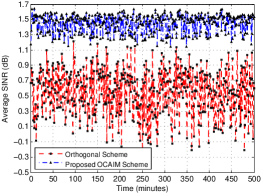
Figure 4: Average SINR versus time of OCAIM with orthogonal TDMA scheme

VII-B SINR versus Interference Threshold

The average SINR versus the interference threshold for OCAIM and that for the smart spectrum allocation SMS and OS schemes are compared. It is observed in Figure 5 that SINR of OCAIM is higher than that of SMS and OS for all interference thresholds.

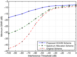
Figure 5: Minimum SINR versus interference threshold of OCAIM with SMS and OS schemes

However, in OS, no coordination is considered (i.e., the probability of superframes overlapping is higher) and neither orthogonal channels nor codes are assigned to the interfering sensors which result in lower values of SINR. On the other side, OCAIM considers interference mitigation not only on a sensor-level as in SMS, but also on a time-slot level, which explains SINR improvement that OCAIM has compared to SMS. Furthermore, in all schemes, a higher SINR is achieved when the interference threshold is increased. Thus, decreasing the interference threshold implies more sensors are added to the interference sets (i.e., more sensors are probably assigned orthogonal codes) which lead to higher SINR values. It is improtant to mention that the work in [8] assigns channels only based on sensor-level interference. In OCAIM, codes are assigned and used by sensors only in some particular time-slots where they experience interference, which explains the improvement in the SINR on other competing schemes.

VII-C WBAN Power Consumption

The power consumption versus time for OCAIM and that for SMS and OS are compared. However, it is clear from Figure 8 that OCAIM has lower power consumption ($0.96\times 10^{-2}mW$) than SMS ($1.3\times 10^{-2}mW$) and OS ($1.6\times 10^{-2}mW$). In OS, the overlapping of active periods results in more collisions, which leads to higher power consumption. Whilst, in SMS, the coordinators negotiate to assign channels to interfering sensors that justifies the decrease in power consumption compared to OS. However, in OCAIM, the coordinators still negotiate to assign codes instead of channels, and so, switching the channel to another consumes more power than code assignments which is confirmed by the simulation results shown in Figure 8, and this justifies the increase in power consumption in SMS. In addition, OCAIM provides a smaller number of sensors that will be assigned codes, which justifies lower consumption than other schemes.

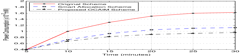
Figure 6: WBAN power consumption versus time

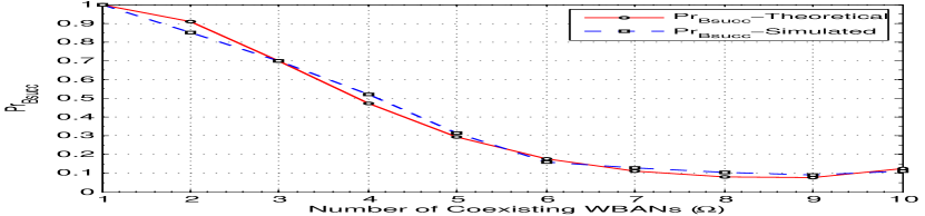
Figure 7: Probability of successful beacon transmission versus WBANs count

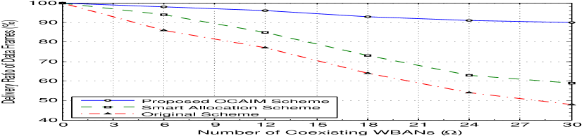
Figure 8: Data frames delivery ratio versus WBANs count

VII-D Beacons Transmission Probability

Figure 8 compares the simulated successful beacon transmission probability denoted by $Pr_{Bsucc}^{simulated}$ and the theoretical probability denoted by $Pr_{Bsucc}^{theoretical}$ with varying the WBANs count. As can be clearly seen in this figure, the simulated probability significantly approaches the theoretical one in all cases, which confirms the validity of the theoretical results.

VII-E WBAN data frames delivery ratio

The data frames delivery ratio denoted by FDR versus WBANs count $(\Omega)$ for OCAIM and that for SMS and OS are compared. Figure 8 shows that FDR of OCAIM is always higher than that of SMS and OS for all values of $\Omega$. However, in OS, the overlapping of active periods results in more collisions due to the absence of coordination and orthogonal channel/code assignments, which leads to lower values of FDR. Whilst, in SMS where the number of channels is limited to 16, the coordinators negotiate to assign channels to interfering sensors that justify the increase in FDR compared to OS. Furthermore, the work in [8] assigns channels only based on sensor-level interference. However, in OCAIM, codes are assigned to sensors only in some particular time-slots where they experience high interference which explains the improvement in FDR on other competing schemes.

VIII Conclusions

In this paper, a distributed orthogonal code allocation scheme is proposed to avoid co-channel interference amongst coexisting WBANs. To the best of our knowledge, we are the first that consider the interference at the sensor- and time-slot- levels. In our proposed scheme, all the sensors and in their assigned time-slots, where they only impose high interference on other WBANs are allocated orthogonal codes, whilst, other sensors are not required to be assigned codes all the time. Furthermore, the proposed scheme mitigates the interference and increases the power savings at sensor- and WBAN-levels, as well as efficiently utilizes the limited resources in WBANs. The performance has been evaluated by extensive experiments and results show the proposed scheme outperforms other competing approaches in terms of interference and power consumption.

References

- [1] Chen, G. Chen, W. and Shen, S., 2L-MAC: A MAC Protocol with Two-Layer Interference Mitigation in Wireless Body Area Networks for Medical Applications, IEEE International Conference on Communications (ICC), pages 3523-3528, 2014
- [2] Ali, M.J. and Moungla, H. and Mehaoua, A., Interference Avoidance Algorithm (IAA) for Multi-hop Wireless Body Area Network Communication, IEEE 17th International Conference on e-Health Networking, Applications and Services (Healthcom 2015) Conference on,pages 1-6, Boston,USA, 2015
- [3] A. Tawfiq and J. Abouei and K. N. Plataniotis, Cyclic orthogonal codes in CDMA-based asynchronous Wireless Body Area Networks, 2012 IEEE International Conference on Acoustics, Speech and Signal Processing (ICASSP), pages 1593-1596, 2012
- [4] Mahapatro, J. and Misra, S. and Manjunatha, M. and Islam, N., Interference mitigation between WBAN equipped patients, Ninth International Conference on Wireless and Optical Communications Networks (WOCN),pages 1-5,2012
- [5] Dong, Jie and Smith, David,Joint relay selection and transmit power control for wireless body area networks coexistence, IEEE International Conference on Communications (ICC), pages 5676-5681, 2014
- [6] Kim, S. and Kim, S. and Kim, J. and Eom, D.,, A beacon interval shifting scheme for interference mitigation in body area networks, Journal Sensors, publisher Molecular Diversity Preservation International, volume 12, number 8, pages 10930–10946, 2012
- [7] Movassaghi, Samaneh and Abolhasan, Mehran and Lipman, Justin and Smith, David and Jamalipour, Abbas, Wireless Body Area Networks: A Survey, IEEE Communications Surveys Tutorials, pages 1658-1686, 2014
- [8] Movassaghi, Samaneh and Abolhasan, Mehran and Smith, David, Smart spectrum allocation for interference mitigation in Wireless Body Area Networks, IEEE International Conference on Communications (ICC), pages 5688-5693, 2014
- [9] S. Movassaghi and A. Majidi and D. Smith and M. Abolhasan and A. Jamalipour, Exploiting Unknown Dynamics in Communications Amongst Coexisting Wireless Body Area Networks, 2015 IEEE Global Communications Conference (GLOBECOM), pages 1-6, 2015
- [10] Shipeng Liang and Yu Ge and Shengming Jiang and Hwee Pink Tan, A lightweight and robust interference mitigation scheme for wireless body sensor networks in realistic environments, IEEE Wireless Communications and Networking Conference (WCNC), pages 1697-1702, 2014
- [11] Dakun, D. and Fengye, H. and Feng, W. and Zhijun, W. and Yu, D. and Lu, W., A game theoretic approach for inter-network interference mitigation in wireless body area networks,journal communications, China, volume 12, number 9, pages 150-161, 2015
- [12] Zou, L. and Liu, B. and Chen, C. and Chen, C.H, Bayesian game based power control scheme for inter-WBAN interference mitigationm Global Communications Conference (GLOBECOM), 2014 IEEE, pages 240-245m 2014
- [13] Movassaghi, S. and Abolhasan, M. and Smith, D. and Jamalipour, A., AIM: Adaptive Internetwork interference mitigation amongst co-existing wireless body area networks, IEEE International Global Communications Conference (GLOBECOM),pages 2460-2465, 2014
- [14] IEEE Standard for Local and metropolitan area networks - Part 15.6: Wireless Body Area Networks,pages 1-271,2012
- [15] Huang, W. and Quek, T.Q.S., Adaptive CSMA/CA MAC protocol to reduce inter-WBAN interference for wireless body area networks, Wearable and Implantable Body Sensor Networks (BSN), 2015 IEEE 12th International Conference on, pages 1-6,2015