Nonequilibrium gas–liquid transition in the driven-dissipative photonic lattice

Abstract

We study the nonequilibrium steady state of the driven-dissipative Bose-Hubbard model with Kerr nonlinearity. Employing a mean-field decoupling for the intercavity hopping $J$, we find that the steep crossover between low and high photon-density states inherited from the single cavity transforms into a gas–liquid bistability at large cavity-coupling $J$. We formulate a van der Waals like gas–liquid phenomenology for this nonequilibrium setting and determine the relevant phase diagrams, including a new type of diagram where a lobe-shaped boundary separates smooth crossovers from sharp, hysteretic transitions. Calculating quantum trajectories for a one-dimensional system, we provide insights into the microscopic origin of the bistability.

I Introduction

The Bose-Hubbard Hamiltonian, describing strongly interacting bosons hopping on a lattice, defines one of the fundamental model systems of condensed matter physics and quantum optics. Its equilibrium phase diagram is characterized by a lobe structure that results from a commensuration effect at integer particle filling per site Fisher1989 . The phase boundary separating superfluid from Mott-insulating phases is well understood Fisher1989 ; Jaksch1998 and has been observed in landmark experiments on cold gases Greiner2002 ; Bakr2010 . Coming to grips with Bose-Hubbard physics remains a challenge in the photonic arena, where drive and dissipation are central to the nonequilibrium model describing a lattice of nonlinear coupled cavities Hartmann2006 . In this paper, we employ a mean-field decoupling in the inter-cavity hopping $J$ on top of the exact single-cavity solution Drummond1980 . We establish a van der Waals like gas–liquid phenomenology and propose a new type of nonequilibrium phase diagram that addresses the nature of the transition between phases. We find a boundary that separates smooth from hysteretic transitions between photonic gas and liquid phases and exhibits a pronounced quantum commensuration effect in the cavity photon number. Quantum trajectories for a chain of cavities show that local density-fluctuations in individual cavities at small $J$ transform into collective super-cavity fluctuations and intermittent light bursts when cavities become strongly coupled at large $J$.

The challenge in understanding the driven lattice roots in the complexity of the single nonlinear cavity with its distinct low and high photon-density states separated by a steep crossover. The experimental observation of bistability between such states in a nonlinear optical device Gibbs1976 triggered a vast amount of theoretical work Carmichael1977 ; Bonifacio1978 ; Drummond1980 ; Gang1990 ; Bishop2010 ; Weimer2015 ; Carmichael2015 ; MendozaArenas2016 ; Casteels2016 ; Minganti2016 . Similar hysteretic cycles have been measured in different platforms and utilized in the context of switching and amplification, e.g., with Josephson junctions Siddiqi2004 and exciton-polaritons in semiconductor microcavities Bajoni2008 ; Amo2010 ; Paraiso2010 ; Rodriguez2016_2 . While such single-cavity physics is now well understood, new research perspectives are being developed to explore bistable behavior in extended systems Eichler2014_2 ; Rodriguez2016 , where the photon hopping $J$ between different cavities competes with the on-site nonlinearity $U$.

Early work on photonic lattices described an (artificial) equilibrium setting with a chemical potential for polaritons Greentree2006 ; Angelakis2007 ; Rossini2007 ; Aichhorn2008 ; Schmidt2009 ; Schmidt2010 , exhibiting close similarities in its phase diagram with that of the massive Bose-Hubbard model Fisher1989 . Furthermore, a proper initialization of the photonic lattice Hartmann2006 , e.g., with an appropriate pump-pulse Tomadin2010_2 , provided signatures for a superfluid–insulator phase transition in a dissipative cavity lattice. Quite different physics emerges, however, when the cavities are coherently driven, breaking the $U(1)$ symmetry explicitly. In this case, a mean-field theory predicts a bistability that takes the array’s state abruptly from low- to high-density phases and vice versa, as was noted for the Jaynes-Cummings-Hubbard model Nissen2012 and similarly for the Bose-Hubbard model with Kerr nonlinearity Boite2013 ; Boite2014 . On the experimental front, a bistable behavior has recently been observed on a large one-dimensional circuit QED array Fitzpatrick2017 , further motivating a deeper understanding of bistable behavior in large lattices.

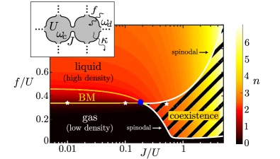
Figure 1: (color online). Mean-field phase diagram of an array of nonlinear cavities with interaction $U$ and loss $\kappa$, pumped with amplitude $f$ at a frequency $\omega_{d}$ detuned from the cavity frequency $\omega_{c}$ by $\Delta=\omega_{d}-\omega_{c}$, see top-left inset. Photons tunnel to neighboring cavities with amplitude $J$. The photon density $n$ at the 4-photon resonance $1+2\Delta/U=4$ is shown as a function of the dimensionless parameters $f/U$ and $J/U$ for small dissipation $\kappa=U/20$. The smooth gas–liquid crossover at small $J/U$ exhibits bimodality (BM region, yellow lines) in the photon number distribution, and gives way to a hysteretic transition at $J_{c}\approx 0.18\,U$ (dot), opening a coexistence region of gas and liquid at $J>J_{c}$ (stripes; colors refer to densities in gas and liquid). The resulting underdriven liquid and overdriven gas phases terminate at the spinodal lines (white), which smoothly extend the lines bounding the bimodal region at small $J$. The stars mark the location of the quantum trajectory results in Fig. 4.

Despite such promising results, no clear view has emerged so far regarding the nature and shape of the nonequilibrium diagram and its relation to the equilibrium Bose Hubbard model, if there exists any at all. In particular, the variety of tunable parameters and drive schemes makes the study of the nonequilibrium photonic lattices a challenging problem. While the hopping $J$ is the obvious choice to track intercavity correlations, the replacement of the chemical potential $\mu$ of the Bose-Hubbard model is less clear. It turns out, that driving the cavities at a frequency $\omega_{d}$ different from the cavity frequency $\omega_{c}$, the detuning $\Delta=\omega_{d}-\omega_{c}$ allows to take the system in and out of many-photon resonances that assume a similar role as the integer site-occupation in the Mott lobes, motivating its use in replacing $\mu$. Finally, imposing a coherent drive $f$, it is the gas–liquid transition with its van der Waals type phenomenology rather than the insulator–superfluid transition that plays the central role in this system.

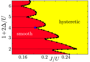
Figure 2: (color online). Mean-field phase diagram displaying the nature of the gas–liquid transition in the driven-dissipative photonic lattice. Plotting the dimensionless detuning $2\Delta/U$ versus hopping $J/U$ at small dissipation $\kappa=U/20$, we show the boundary separating smooth from hysteretic gas–liquid transitions as driven by increasing the pump amplitude $f$. Distinct lobes appear between successive $m$-photon resonances of the individual cavities, i.e., when $1+2\Delta/U=m$ assumes an integer value, thus featuring a similar commensuration effect as the equilibrium Bose-Hubbard model. Going to small $\Delta/U$ or very small dissipation $\kappa$, instabilities show up in the mean-field analysis, see also Refs. Boite2013 ; Wilson2016 . Numerical errors are of order the size of the points.

In our analysis, we make use of a mean-field decoupling scheme in the hopping $J$. Such a mean-field description has been very successful in predicting the qualitative features of the equilibrium phase diagram of the Bose-Hubbard model, motivating its use for the investigation of our nonequilibrium setting as well. The results of our analysis are expressed in two phase diagrams. Fig. 1 shows how the gas–liquid transition as driven by the coherent pump amplitude $f$ changes from a steep crossover inherited from the single cavity at small $J$ to a first-order type hysteretic or bistable transition at large $J$. The termination of the hysteretic behavior upon decreasing $J$ then defines a critical end-point to a first-order like transition in the $f$–$J$ diagram at fixed detuning $\Delta$. In Fig. 2, we track the location of this critical end-point in a $\Delta$–$J$ diagram and find a boundary with characteristic lobes appearing between successive $m$-photon resonances of the individual cavities where $1+2\Delta/U=m$ assumes integer values. This boundary separates regions where the gas–liquid transition is smooth (small $J/U$) from regions where bistability governs the lattice’s behavior as the pump amplitude $f$ is tuned across the transition. Contrary to conventional phase diagrams describing transitions between phases, our $\Delta$–$J$ phase diagram addresses the nature of the transition, smooth versus hysteretic, as the system parameters are changed.

II Driven-Dissipative Bose-Hubbard Model

We consider the driven-dissipative Bose-Hubbard (BH) model, describing photons hopping on a lattice of nonlinear cavities, pumped and lossy. The Hamiltonian ($\hbar=1$) reads

$$H=\sum_{i}h^{\scriptscriptstyle\rm BH}_{i}+\frac{1}{z}\sum_{\langle ij\rangle}J_{ij}a^{\dagger}_{i}a_{j}$$ (1)

with $h^{\scriptscriptstyle\rm BH}_{i}=-\Delta\,n_{i}+Un_{i}(n_{i}-1)/2+f(a_{i}+a_{i}^{\dagger})$, the bosonic operators $a_{i}$ and the number operators $n_{i}=a^{\dagger}_{i}a_{i}$. Each site $i$ is coherently pumped with strength $f$ as described by the last term in $h^{\scriptscriptstyle\rm BH}_{i}$. In a frame rotating with the drive frequency $\omega_{d}$, the cavity frequency is renormalized to $\Delta=\omega_{d}-\omega_{c}$, while $U$ is the local Kerr nonlinearity. The second term in $H$ describes the hopping to $z$ nearest-neighbor cavities with amplitude $J_{ij}=-J$; the factor $1/z$ in Eq. (1) ensures a bandwidth $2J$ independent of $z$ and guarantees a regular limit $z\to\infty$ where mean-field theory becomes exact. The dissipative dynamics for the density matrix $\rho$ is determined by the Lindblad master equation

$$\dot{\rho}=-i[H,\rho]+\frac{\kappa}{2}\sum_{i}(2a_{i}\rho a_{i}^{\dagger}-a_{i}^{\dagger}a_{i}\rho-\rho a_{i}^{\dagger}a_{i}),$$ (2)

with the photon decay rate $\kappa$. Models of this type can be realized in quantum engineered settings using superconductor- Houck2012 ; Schmidt2013_2 ; Leib2014 and semiconductor technologies Carusotto2013 ; Baboux2015 .

II.1 Single Cavity

The driven-dissipative single cavity (i.e., equation (2) with $J=0$) has been solved exactly by Drummond and Walls Drummond1980 and the results are summarized in Fig. 3. The diagram in Fig. 3(a) exhibits two states or phases characterized by low and high photon-densities $n=\langle a^{\dagger}a\rangle$. The crossover from the low- (gas) to the high-density (liquid) phase is driven via increasing the pumping amplitude $f$ and exhibits bimodality in the photon number distribution $p_{k}$, see also Ref. Fink2016 . We estimate the location of the crossover line by comparing terms in the Hamiltonian $h^{\scriptscriptstyle\rm BH}$, generating scalings $n\sim(f/\Delta)^{2}$ at small drive $f$ (gas-phase) and $n\sim(f/U)^{2/3}$ in the liquid phase at large $f$ where the interaction $U$ dominates. The crossover between the two regimes appears at $n\sim\Delta/U$ and defines the crossover line $f^{\mathrm{sc}}_{\!\scriptscriptstyle\times}/U\sim(\Delta/U)^{3/2}$. We obtain a more quantitative result from the exact solution Drummond1980 at weak dissipation $\kappa/U\ll 1$: with the compressibility $K=1+n(g^{\scriptscriptstyle(2)}-1)$ dropping below unity upon entering the liquid phase ($g^{\scriptscriptstyle(2)}=\langle a^{\dagger}a^{\dagger}aa\rangle/n^{2}$ the second-order coherence), the condition $K=1$ provides the result $f^{\mathrm{sc}}_{\!\scriptscriptstyle\times}/U\approx(m/2e)^{3/2}(m\kappa/U)^{1/m}$ at the $m$-photon resonance $2\Delta=(m-1)\,U$ (where the energy of $m$ photons outside and inside the cavity match up), which agrees (up to a numerical coefficient) with our previous estimate at large $m$.

The interaction leads to an intermediate plateau in the liquid phase with density $n\approx\Delta/U$, see inset in Fig. 3(b) (the $1/2$ reduction in $n$ with respect to $m$ is a saturation effect Biondi2015 ). The transition to the liquid is helped when the drive frequency is resonant with the $m$-photon state of the cavity at $2\Delta/U=(m-1)$, yielding the modulation of the crossover line in Fig. 3, see also Ref. Carmichael2015 . The low- and high-density phases are well described by coherent states (except for small $f$ and $\Delta$) as quantified by the correlator $g^{\scriptscriptstyle(2)}$. The crossover in between is characterized by large density fluctuations and superbunching, see Fig. 3(b).

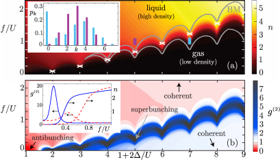
Figure 3: (color online). Density $n$ (a) and second-order coherence $g^{\scriptscriptstyle(2)}$ (b) as a function of drive detuning $2\Delta/U$ and drive strength $f/U$ for a single cavity as obtained from the exact solution Drummond1980 of equation (2) with $J=0$ and $\kappa=U/20$. The modulated grey lines labelled ‘BM’ encompass the bimodal regime. The inset displays the photon number distribution $p_{k}$ at the two bars marked in the main panel. The white crosses mark the onset $f^{\mathrm{sc}}_{\!\scriptscriptstyle\times}$ of the liquid phase as defined by the condition of unit compressibility $K=1$. The correlator $g^{\scriptscriptstyle(2)}$ illustrates the phases’ coherent nature, while the crossover is characterized by superbunching, see also Ref. Fitzpatrick2017 . The bottom inset displays the density $n$ and correlator $g^{\scriptscriptstyle(2)}$ evaluated at fixed detunings $2\Delta/U=3,~{}3.5$ (solid, dashed).

II.2 Cavity Lattice

We now combine cavities into a lattice and increase the intercavity hopping $J$. We solve for the non-equilibrium steady state $\dot{\rho}=0$ of the photonic lattice by reducing the task to a single-site problem via a mean-field decoupling of the hopping term Tomadin2010_2 ; Tomadin2011 in equation (2), i.e, $a^{\dagger}_{i}a_{j}\approx\langle a^{\dagger}_{i}\rangle a_{j}+a^{\dagger}_{i}\langle a_{j}\rangle-\langle a_{i}^{\dagger}\rangle\langle a_{j}\rangle$; the same decoupling has been used in the equilibrium model Fisher1989 and provided correct qualitative results for the phase diagram. Alternatively, the same approximation can be obtained from an expansion of the lattice density matrix in inverse powers of the coordination number $z$ Navez2010 ; truncating the expansion at order unity is equivalent to the mean-field decoupling of the hopping term and is exact in the limit $z\rightarrow\infty$, i.e., large dimensions. We then obtain a self-consistent equation Drummond1980 ; Boite2013 for the mean amplitude $\langle a_{i}\rangle=\langle a\rangle$,

$$\langle a\rangle=-\frac{2|\varphi_{J}|}{\delta}\frac{{}_{0}F_{2}(;1+\delta,\delta^{\ast};8|\varphi_{J}|^{2})}{{}_{0}F_{2}(;\delta,\delta^{\ast};8|\varphi_{J}|^{2})},$$ (3)

with the renormalized drive $\varphi_{J}=(f-J\langle a\rangle)/U$ depending on $\langle a\rangle$, the dimensionless detuning $\delta=-(2\Delta+i\kappa)/U$ and the hypergeometric function ${}_{0}F_{2}(;a,b;z)$; the solution for $\langle a\rangle$ provides direct access to the photon density $n=\langle a^{\dagger}_{i}a_{i}\rangle=\langle a^{\dagger}a\rangle$ and higher-order correlators Drummond1980 . Eq. (3) exhibits multiple solutions at large hopping $J$. The location $J_{c}$ where these multiple solutions first show up is our main interest here, since it describes the transition from a smooth gas–liquid crossover in the density $n$ as observed in the single cavity, to a hysteretic first-order type transition characteristic of a strongly-coupled lattice system.

The driven Bose-Hubbard model involves the parameters $f$, $U$, $J$, and $\Delta$, and it is the suitable choice within this set which brings forward the properties of this system. In a first step, we fix the dimensionless detuning $\Delta/U$ to the four-photon resonance at $1+2\Delta/U=4$ and increase the drive $f/U$. This produces the gas–liquid phase diagram in Fig. 1, where the density $n$ assumes the role of the order parameter. At small hopping $J/U<0.18$, gas and liquid phases are separated by a steep crossover with a bimodal distribution $p_{k}$ of photon numbers inherited from the single cavity. The location of this crossover is well described by the compressibility criterion $K=1$, resulting in a line following accurately the upper boundary of the bimodal region in Fig. 1; an approximation in the small-$\kappa$ limit Boite2014 yields a linear dependence on $J$,

$$f_{\!\scriptscriptstyle\times}\approx f_{\!\scriptscriptstyle\times}^{\mathrm{sc}}(1-2J/U),$$ (4)

with $f^{\mathrm{sc}}_{\!\scriptscriptstyle\times}$ the single-cavity expression derived with the same condition $K=1$. The smooth crossover between gas and liquid phases ends at a ‘critical’ value $J_{c}\approx 0.18\,U$ (blue dot), corresponding to $f_{c}\approx 0.29\,U$, giving way to a hysteretic transition at larger hopping $J/U$ that shows the signatures typical of a van der Waals like gas–liquid transition Domb1996 : using this terminology, we find two-phase coexistence bounded by spinodal lines at large coupling $J$ that smoothly develop out of the bimodal lines at small coupling. Similar results are obtained at different values of the misfit parameter $\Delta/U$, but with a plateau at a suitably adapted photon density, $n\approx\Delta/U$.

Evaluating the location of the critical point $J_{c}$ for different detunings $\Delta/U$, we can plot a boundary separating smooth from hysteretic behavior and arrive at a complete characterization of the system. We find a boundary with a lobe-like structure that is commensurate with the $m$-photon resonances at integer values of $1+2\Delta/U$, see Fig. 2, a result that has been searched for in the past, but has remained elusive so far.

III Quantum Trajectories

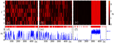
Figure 4: (color online). Selected quantum trajectories for a 1D cavity array with 6 sites. The panels (a)–(c) show the photon density in color scale as a function of time ($t\kappa$) and position (lattice site $j$) at fixed drive strength $f/U=0.35$ and for increasing hopping $J/U$ as marked with the stars in the phase diagram of Fig. 1. At small hopping $J\ll J_{c}$, the trajectories of different sites are uncorrelated (a), while for $J>J_{c}$, the entire cavity array switches collectively between gas and liquid states within the coexistence region of the mean-field diagram, see (c). The panels (d)–(f) show trajectories for a single lattice site $j=4$ as a function of time, as taken from the respective top panels (a)–(c). The vertical red bars indicate the photon emissions from the lattice. For $J\ll J_{c}$ (d) each individual cavity displays intermittency Plenio1998 (see also text) at random times, yielding a constant photon emission from the array. For $J>J_{c}$ (f) the array behaves as a coherent super-cavity and a collective intermittency is restored. The horizontal arrows mark the gas and liquid mean-field values, showing that collective switching in panel (c) indeed occurs between the mean-field densities. Panels (a), (b), (c): $J/U=0.01,0.1,0.5$. Other parameters are chosen as in Fig. 1. Convergence of the quantum trajectory results in the photon truncation parameter (cutoff) is illustrated in Appendix B.

In order to substantiate our results, we complete this study with a microscopic view on the gas–liquid diagram in Fig. 1. In Fig. 4, we present simulation results of selected quantum trajectories Dalibard1992 ; Carmichael1992 (see also the reviews Plenio1998 ; Daley2014 and the Appendix A for further information) for a chain of 6 nonlinear cavities in one dimension (1D) with periodic boundary conditions. At small values of $J$, the cavities switch individually between gas and liquid states, see panel (a), with a rapidly growing weight of the liquid when $f$ is tuned across $f_{\!\scriptscriptstyle\times}/U\sim(\Delta/U)^{3/2}$. As $J/U$ is increased within the bimodal region, the fluctuations become correlated and extended super-cavities are formed, see panel (b). Increasing $J$ further across $J_{c}$, the entire strongly-coupled array switches collectively as illustrated by the appearance of pronounced stripes in panel (c) of Fig. 4, with switching times largely exceeding those of the individual cavities. In an infinite system, we then expect a second-order transition with a diverging correlation length to appear as $J$ is increased towards $J_{c}$ in the bimodal strip. This hypothesis is supported by simulations exhibiting a rapid increase of the collective switching time with system size, suggesting a closing of the Liouvillian gap in the thermodynamic limit (see Appendix C), and invites for further exploration, also with a view on the role of lattice dimensionality FossFeig2017 . On the other hand, increasing the drive $f$ at fixed coupling $J>J_{c}$, we expect a first-order type behavior with nucleation of extended liquid phases in the gas and vice versa on decreasing $f$. The intermittent light bursts appearing in the hysteretic regime, cf. the red photon emission processes shown in Fig. 4(f), naturally show up in the context of dynamical phase transitions Ates2012 and can serve as an experimental probe of the hysteretic behavior Fitzpatrick2017 . We note that quantum trajectories obtained in related models, assemblies of Rydberg atoms Ates2012 ; Lee2012 and spin-1/2 $XY$ models Wilson2016 , also exhibit collective switchings between phases but do not show individual fluctuations with a transition between the two behaviors.

In comparing the physics of the two versions of the Bose-Hubbard model, equilibrium versus coherently-driven–dissipative, we note that the former is characterized by a phase boundary $J_{c}(\mu)$ describing a spontaneous breaking of $U(1)$ symmetry, while the latter exhibits the phenomenology of a tunable van der Waals type gas–liquid transition. In particular, in the coherently driven system, the $U(1)$ symmetry is explicitly broken and the interesting feature is the transformation of a smooth crossover into a hysteretic transition involving local (at small $J$) or collective (at large $J$) temporal fluctuations of low- and high-density phases. In spite of the differences between the two phenomenologies, both phase boundaries $J_{c}(\mu)$ and $J_{c}(\Delta)$ exhibit a particle commensuration effect resulting in a lobe-like structure. In the equilibrium situation, the superfluid phase is favored whenever the chemical potential $\mu$ allows for two different particle numbers, while in the driven Bose-Hubbard model, a detuning $\Delta$ matching a many-photon resonance in each cavity facilitates their synchronization and thereby triggers collective jumps between gas- and liquid photonic phases. This can be understood as a variation of Le Chatelier’s principle stating that the system reacts to a disturbance, here a change in $\mu$ or $\Delta$, by favoring the corresponding phase, superfluid when particle number becomes undefined and intermittent light bursts when approaching a resonance.

IV Summary and Conclusions

Summarizing, we have presented a mean-field analysis of the driven-dissipative Bose-Hubbard model describing a lattice of coupled nonlinear cavities. Inspired by the exact single-cavity solution with its crossover between low- and high-density phases, we have established a van der Waals type gas–liquid phenomenology for the driven photonic Bose-Hubbard model featuring a change from smooth to hysteretic transition upon increasing the coupling $J$ beyond critical. A quantum-trajectory analysis shows that the bistable region involves collective switching between gas- and liquid phases triggering bursts of light. Choosing the correct representation in parameter space, both equilibrium and driven phase diagrams exhibit boundaries with a lobe-like structure that originates from a resonance condition in the on-site Hamiltonian. We expect that models with a similar on-site nonlinearity, e.g., the Jaynes-Cummings-Hubbard model Greentree2006 ; Nissen2012 will exhibit an analogous phase diagram, while models of similar kind, e.g., assemblies of Rydberg atoms and spin-1/2 systems MendozaArenas2016 ; Ates2012 ; Lee2012 ; Wilson2016 , will benefit from the insights obtained in this paper. Our results clarify a long-standing problem on the nature and shape of the phase diagram of the driven Bose-Hubbard model and guide new experiments on photonic arrays.

Appendix A Quantum trajectory approach

In here, we briefly summarize the quantum trajectory algorithm introduced in the Refs. Dalibard1992 and Carmichael1992 and well documented in reviews, see, e.g., Refs. Plenio1998 and Daley2014 . The algorithm is used to describe open quantum systems whose dynamics is described by a master equation in Lindblad form, as Eq. (2) in the main text. The quantum trajectory method is, (i) numerically advantageous with respect to the direct integration of the master equation, and (ii) can provide further insight into the dynamical behavior of the system due to the stochastic nature of the trajectories. The algorithm stochastically propagates the wavefunction $\ket{\psi(t)}$ under the non-hermitian Hamiltonian

$$H_{\rm eff}=H-i\frac{\kappa}{2}\sum_{j}a^{\dagger}_{j}a_{j}$$ (5)

with the photon decay rate $\kappa$. The Hamiltonian $H$ of Eq. (5), the density operator $n_{j}=a^{\dagger}_{j}a_{j}$ and the photon operator $a_{j}$ have been introduced in Eq. (1) of the main text. The algorithm can be summarized as follows. If in the time interval $[t,t+dt]$ the cavity at site $j$ emits a photon, the wavefunction collapses to $\ket{\psi(t+dt)}=a_{j}\ket{\psi(t)}$, while, if no photon is emitted, $\ket{\psi(t+dt)}=(1-iH_{\rm eff}\,dt)\ket{\psi(t)}$. Which of these events occurs depends on the photon density $n_{j}(t)=\braket{\psi(t)}{n_{j}}{\psi(t)}$ and is determined stochastically by comparison with a random number. This process can be understood as the measurement of the system by the environment. This follows from the fact that information is gained also when no photon is emitted. After normalizing the wavefunction, the stochastic evolution continues with the next time step till the trajectory is complete. In practice, variants of the algorithm of higher order in the time step $dt$ are used Daley2014 .

The quantum trajectory algorithm is numerically advantageous with respect to the direct integration of the master equation, since it is based on propagating the wavefunction instead of the density matrix; furthermore, different trajectories are independent and can thus be propagated in parallel. The average over different stochastic evolutions is equivalent to the density matrix dynamics as determined by the Lindblad master equation given by Eq. (2) of the main text. Furthermore, in the single trajectories fundamental information on the behavior of the system is revealed.

Appendix B Convergence in the photon truncation parameter

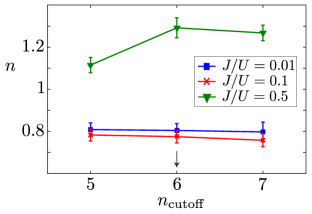
Figure 5: (color online). Convergence plot of the average photon density $n$ (see Eq. (6)) in the steady state for various values of hopping strengths $J/U$ as calculated with quantum trajectories. The average density $n$ is shown as a function of the photon number truncation parameter $n_{\rm cutoff}$ for a lattice of $N=5$ sites with PBC. The vertical bars denote one standard deviation (see text). Other parameters as in Fig. 4 of the main text. The vertical arrow indicates the cutoff value $n_{\rm cutoff}=6$ used in Fig. 4 of the main text, for an array of $N=6$ sites with PBC.

To obtain Fig. 4 in the main text, we employ a 5-th order Runge-Kutta (built in the Matlab routine ode45) to simulate the stochastic evolution as outlined in Section 3.5 of Ref. [Daley2014, ]. For the quantum trajectories displayed in Fig. 4 of the main text, up to 6 photons per cavity are admitted, resulting in a Hilbert space of $7^{6}=117649\approx 2^{17}$ states. Fig. 5 shows the convergence of the average photon density as a function of the photon number truncation parameter $n_{\rm cutoff}$ for different $J/U$ values for a lattice of $N=5$ sites with periodic boundary conditions (PBC). The average photon density is defined as

$$\begin{split}n&=\langle\langle\langle n\rangle_{\rm time}\rangle_{\rm sites}\rangle_{\rm traj}\\ &=\frac{1}{N_{\rm traj}N_{\rm sites}N_{\rm t\text{-}steps}}\sum_{r=1}^{N_{\rm traj}}\sum_{j=1}^{N_{\rm sites}}\sum_{t=t_{0}}^{N_{\rm t\text{-}steps}}n_{j,r,t}.\end{split}$$ (6)

In the definition above, the average is taken first over time for $t\geq t_{0}$, with $t_{0}\gg 1/\kappa$ such that a steady state is reached; the resulting density is averaged over different sites in the lattice and finally an average over the results obtained through independent trajectories is performed. The squared deviation from the mean (variance) is propagated according to the standard prescriptions of error propagation, yielding a final standard deviation $\sigma_{n}$. In the coexistence region of the mean-field (see main text) where the different sites in the array are correlated, only a specific site $j=4$ is considered and the average over different sites is discarded. In our convergence simulations, $N_{\rm t\text{-}steps}\approx 10^{4}$, $N_{\rm traj}=100$ and $N_{\rm sites}=N=5$. At small $J/U$ (blue and red symbols) we note that already $n_{\rm cutoff}=5$ provides a good approximation. At larger hopping strengths (green symbols) we find that a larger cutoff is needed to reach convergence within one standard deviation.

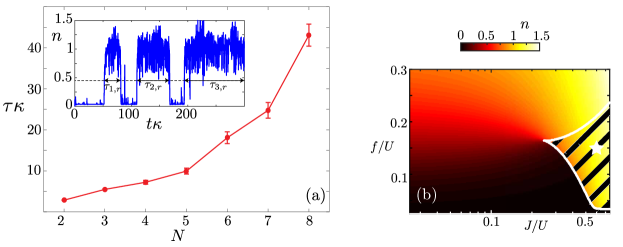
Figure 6: (color online). Collective time spent in the liquid phase $\tau$ (see Eq. (7) and main text) in the steady state as calculated with quantum trajectories (QT) as a function of the size $N$ of a one-dimensional array with PBC (a). The inset displays a sample trajectory for $N=8$ exhibiting 3 separate periods where the system dwells in the liquid phase (see also text). In order to extract $\tau_{s,r}$ (see text), an arbitrary threshold $n=0.4$ is used to separate gas and liquid phases and density fluctuations on a scale smaller than $dt=2/\kappa$ are neglected. We have checked that the trend in the results (exponential-like increase of $\tau$ with $N$) is invariant with respect to these choices. The trajectory results are shown for a set of parameters within the coexistence region of the mean-field (MF), $f/U=0.15$, $J/U=0.6$, as indicated by the white star in (b). The detuning value $\Delta=\omega_{d}-\omega_{c}$ (detuning between the drive frequency and the cavity frequency) is set to $1+2\Delta/U=1.55$. For this choice of detuning, convergence of the quantum trajectory results in the photon truncation parameter $n_{\rm cutoff}$ is achieved for $n_{\rm cutoff}=3$, much lower than $n_{\rm cutoff}=6$ required for the detuning value $1+2\Delta/U=4$ used in Figs. 1 and 4 in the main text. The choice of a lower detuning $\Delta/U$ with respect to Fig. 4 in the main text thus allows us to study larger system sizes. The dissipation strength is chosen as $\kappa/U=20$, as in Figs. 1–4 in the main text.

Appendix C Scaling of the collective switching time with system size

In this section we focus on the coexistence region of the mean-field (see main text) and discuss the scaling of the collective switching time (see main text) with system size as calculated with quantum trajectories. To this end we consider the average time $\tau$ spent in the liquid phase; in order to extract $\tau$ from an ensemble of trajectories we first obtain the average time spent in the liquid phase in a single trajectory and successively average the result over different trajectories, i.e.,

$$\tau=\langle\langle\tau\rangle_{\rm time}\rangle_{\rm traj}=\frac{1}{N_{\rm traj}}\sum_{r=1}^{N_{\rm traj}}\frac{1}{N_{\rm liquid}(r)}\sum_{s=1}^{N_{\rm liquid}(r)}\tau_{s,r}.$$ (7)

In the definition above $\tau_{s,r}$ is the time spent in the liquid phase in trajectory $r$ and in period $s$; the number of separate periods where the system dwells in the liquid phase in each trajectory is denoted by $N_{\rm liquid}(r)$ and is trajectory-dependent. The squared deviation from the mean (variance) is propagated according to the standard prescriptions of error propagation, yielding a final standard deviation $\sigma_{\tau}$. In these simulations $N_{\rm traj}=150$. Fig. 6(a) shows $\tau$ (7) as a function of system size for a set of parameters within the coexistence region of the mean-field, see Fig. 6(b). The inset in Fig. 6(a) shows a sample trajectory characterized by 3 separate periods; when the system is still in the liquid phase at the end of the trajectory, the latter is considered as the end of the period. We find that the the time spent in the liquid phase increases rapidly with system size; this result is consistent with our hypothesis on the emergence of a transition in the thermodynamic limit characterized by a closing of the Liouvillian gap (see main text).

References

- (1) M. P. A. Fisher, P. B. Weichman, G. Grinstein, and D. S. Fisher, Phys. Rev. B 40, 546 (1989).
- (2) D. Jaksch, C. Bruder, J. I. Cirac, C. W. Gardiner, and P. Zoller, Phys. Rev. Lett. 81, 3108 (1998).
- (3) M. Greiner, O. Mandel, T. Esslinger, T. W. Hänsch, and I. Bloch, Nature 415, 39 (2002).
- (4) W. S. Bakr, A. Peng, M. E. Tai, R. Ma, J. Simon, J. I. Gillen, S. Foelling, L. Pollet, and M. Greiner, Science 329, 547 (2010).
- (5) M. J. Hartmann, F. G. S. L. Brandão, and M. B. Plenio, Nat. Phys. 2, 849 (2006).
- (6) P. D. Drummond and D. F. Walls, J. Phys. A: Math. Gen. 13, 725 (1980).
- (7) H. M. Gibbs, S. L. McCall, and T. N. C. Venkatesan, Phys. Rev. Lett. 36, 1135 (1976).
- (8) H. J. Carmichael and D. F. Walls, J. Phys. B: At. Mol. Phys. 10, L685 (1977).
- (9) R. Bonifacio and L. A. Lugiato, Phys. Rev. A 18, 1129 (1978).
- (10) H. Gang, C. -Z. Ning, and H. Haken, Phys. Rev. A 41, 3975 (1990).
- (11) L. S. Bishop, E. Ginossar, and S. M. Girvin, Phys. Rev. Lett. 105, 100505 (2010).
- (12) H. Weimer, Phys. Rev. Lett. 114, 040402 (2015).
- (13) H. J. Carmichael, Phys. Rev. X 5, 031028 (2015).
- (14) J. J. Mendoza-Arenas, S. R. Clark, S. Felicetti, G. Romero, E. Solano, D. G. Angelakis, and D. Jaksch, Phys. Rev. A 93, 023821 (2016).
- (15) W. Casteels, F. Storme, A. Le Boité, and C. Ciuti, Phys. Rev. A 93, 033824 (2016).
- (16) F. Minganti, N. Bartolo, J. Lolli, W. Casteels, and C. Ciuti, Sci. Rep. 6, 26987 (2016).
- (17) I. Siddiqi, R. Vijay, F. Pierre, C. M. Wilson, M. Metcalfe, C. Rigetti, L. Frunzio, and M. H. Devoret, Phys. Rev. Lett. 93, 207002 (2004)
- (18) D. Bajoni, E. Semenova, A. Lemaître, S. Bouchoule, E. Wertz, P. Senellart, S. Barbay, R. Kuszelewicz, and J. Bloch, Phys. Rev. Lett. 101, 266402 (2008).
- (19) A. Amo, T. C. H. Liew, C. Adrados, R. Houdré, E. Giacobino, A. V. Kavokin, and A. Bramati, Nat. Photon. 4, 361 (2010).
- (20) T. K. Paraïso, M. Wouters, Y. Léger, F. Morier-Genoud, and B. Deveaud-Plédran, Nat. Mater. 9, 655 (2010).
- (21) S. R. K. Rodriguez, W. Casteels, F. Storme, I. Sagnes, L. Le Gratiet, E. Galopin, A. Lemaître, A. Amo, C. Ciuti, and J. Bloch, arXiv:1608.00260 (2016).
- (22) C. Eichler, Y. Salathe, J. Mlynek, S. Schmidt, and A. Wallraff, Phys. Rev. Lett. 113, 110502 (2014).
- (23) S. R. K. Rodriguez, A. Amo, I. Sagnes, L. Le Gratiet, E. Galopin, A. Lemaître, and J. Bloch, Nat. Comm. 7, 1 (2016).
- (24) A. D. Greentree, C. Tahan, J. H. Cole, and L. Hollenberg, Nat. Phys. 2, 856 (2006).
- (25) D. G. Angelakis, M. F. Santos, and S. Bose, Phys. Rev. A 76, 031805 (2007).
- (26) D. Rossini and R. Fazio, Phys. Rev. Lett. 99, 186401 (2007).
- (27) M. Aichhorn, M. Hohenadler, C. Tahan, and P. B. Littlewood, Phys. Rev. Lett. 100 216401, (2008).
- (28) S. Schmidt and G. Blatter, Phys. Rev. Lett. 103, 086403 (2009).
- (29) S. Schmidt and G. Blatter, Phys. Rev. Lett. 104, 216402 (2010).
- (30) A. Tomadin, V. Giovannetti, R. Fazio, D. Gerace, I. Carusotto, H. E. Türeci, and A. Imamoglu, Phys. Rev. A 81, 061801 (2010).
- (31) F. Nissen, S. Schmidt, M. Biondi, G. Blatter, H. E. Türeci, and J. Keeling, Phys. Rev. Lett. 108, 233603 (2012).
- (32) A. Le Boité, G. Orso, and C. Ciuti, Phys. Rev. Lett. 110, 233601 (2013).
- (33) A. Le Boité, G. Orso, and C. Ciuti, Phys. Rev. A 90, 063821 (2014).
- (34) M. Fitzpatrick, N. M. Sundaresan, A. C. Y. Li, J. Koch, and A. A. Houck, Phys. Rev. X 7, 011016 (2017).
- (35) A. A. Houck, H. E. Türeci, and J. Koch, Nat. Phys. 8, 292 (2012).
- (36) S. Schmidt and J. Koch, Ann. der Physik 525, 395 (2013).
- (37) M. Leib and M. J. Hartmann, Phys. Rev. Lett. 112, 223603 (2014).
- (38) I. Carusotto and C. Ciuti, Rev. Mod. Phys. 85, 299 (2013).
- (39) F. Baboux, L. Ge, T. Jacqmin, M. Biondi, E. Galopin, A. Lemaître, L. Le Gratiet, I. Sagnes, S. Schmidt, H. E. Türeci, A. Amo, and J. Bloch, Phys. Rev. Lett. 116, 066402 (2016).
- (40) J. M. Fink, A. Dombi, A. Vukics, A. Wallraff, and P. Domokos, Phys. Rev. X 7, 011012 (2017).
- (41) M. Biondi, E. P. L. van Nieuwenburg, G. Blatter, S. D. Huber, and S. Schmidt, Phys. Rev. Lett. 115, 143601 (2015).
- (42) A. Tomadin, S. Diehl, and P. Zoller, Phys. Rev. A 83, 013611 (2011).
- (43) P. Navez and R. Schützhold, Phys. Rev. A 82, 063603 (2010).
- (44) C. Domb, The Critical Point: A Historical Introduction To The Modern Theory Of Critical Phenomena, (CRC Press, 1996).
- (45) J. Dalibard, Y. Castin, and K. Molmer, Phys. Rev. Lett. 68, 580–583 (1992).
- (46) L. Tian and H. J. Carmichael, Phys. Rev. A. 46, R6801 (1992).
- (47) M. B. Plenio and P. L. Knight, Rev. Mod. Phys. 70, 1 (1998).
- (48) A. J. Daley, Adv. Phys. 63, 77-149 (2014).
- (49) M. Foss-Feig, P. Niroula, J. T. Young, M. Hafezi, A. V. Gorshkov, R. M. Wilson, and M. F. Maghrebi, Phys. Rev. A 95, 043826 (2017).
- (50) C. Ates, B. Olmos, J. P. Garrahan, and I. Lesanovsky, Phys. Rev. A 85, 043620 (2012).
- (51) T. E. Lee, H. Häffner, and M. C. Cross, Phys. Rev. Lett. 108, 023602 (2012).
- (52) R. M. Wilson, K. W. Mahmud, A. Hu, A. V. Gorshkov, M. Hafezi, and M. Foss-Feig, Phys. Rev. A 94, 033801 (2016).