Engagement dynamics and sensitivity analysis of YouTube videos

Abstract

YouTube, with millions of content creators, has become the preferred destination for watching videos online. Through the Partner program, YouTube allows content creators to monetize their popular videos. Of significant importance for content creators is which meta-level features (e.g. title, tag, thumbnail) are most sensitive for promoting video popularity. The popularity of videos also depends on the social dynamics, i.e. the interaction of the content creators (or channels) with YouTube users. Using real-world data consisting of about $6$ million videos spread over $25$ thousand channels, we empirically examine the sensitivity of YouTube meta-level features and social dynamics. The key meta-level features that impact the view counts of a video include: first day view count , number of subscribers, contrast of the video thumbnail, Google hits, number of keywords, video category, title length, and number of upper-case letters in the title respectively and illustrate that these meta-level features can be used to estimate the popularity of a video. In addition, optimizing the meta-level features after a video is posted increases the popularity of videos. In the context of social dynamics, we discover that there is a causal relationship between views to a channel and the associated number of subscribers. Additionally, insights into the effects of scheduling and video playthrough in a channel are also provided. Our findings provide a useful understanding of user engagement in YouTube.

1 Introduction

The YouTube social network contains over 1 billion users who collectively watch millions of hours of YouTube videos and generate billions of views every day. Additionally, users upload over $300$ hours of video content every minute. YouTube generates billions in revenue through advertising and through the Partner program shares the revenue with the content creators.

The video view count is a key metric of the measure of popularity or “user engagement” of a video and the metric by which YouTube pays the content providers. A key question is: How do meta-level features of a posted video (e.g. thumbnail, title, tags, description) drive user engagement in the YouTube social network? However, the content alone does not influence the popularity of a video. YouTube also has a social network layer on top of it’s media content. The main social component is how the content creators (also called “channels”) interact with the users. So another key question is: How does the interaction of the YouTube channel with the user affect popularity of videos? In this paper, we study both the above questions. In particular, our aim is to examine how the individual video features (through the meta-level data) and the social dynamics contribute to the popularity of a video.

Literature Review

The study of popularity of YouTube videos based on meta-level features is a challenging problem given the diversity of users and content providers. Several models on characterizing the popularity of YouTube videos are parametric in form, where the view count time series is used to estimate the model parameters. For example, ARMA time series models [1], multivariate linear regression models [2], modified Gompertz models [3, 4], have been utilized to estimate the future video view counts given past view count time series. Using only the title of the video (one of the meta-level features) [5] considers the problem of predicting whether the view count will be high or low. In a related context, [6, 7] studied the importance of tags for Flicker data. Aside from text based meta-level features (title and tags), in [8] Support Vector Regression (SVR) is proposed to predict the popularity using features of the video frames (e.g. face present, rigidity, color, clutter). It is illustrated in [8] that using the combination of visual features and temporal dynamics results in improved performance of the SVR for predicting view count compared to using only visual features or temporal dynamics alone. In the social context, the uploading behaviour of YouTube content creators was studied in [9]. Specifically, the paper finds that YouTube users with a social network are more popular compared to other users.

Main results

In this paper, we investigate how the meta-level features and the interaction of the YouTube channel with the users affect the popularity of videos. For convenience we summarize the main empirical conclusions of this paper:

1. The five dominant meta-level features that affect the popularity of a video are: first day view count , number of subscribers, contrast of the video thumbnail, Google hits, and number of keywords. Sec. 2 discusses this further.

2. Optimizing the meta-level features (e.g. thumbnail, title, tags, description) after a video has been posted increases the popularity of the video. In addition, optimizing the title increases the traffic due to YouTube search, optimizing the thumbnail increases the traffic from related videos and optimizing the keywords increases the traffic from related and promoted videos. Sec. 2.4 provides details on this analysis.

3. Insight into the causal relationship between the subscribers and view count for YouTube channels is also explored. For popular YouTube channels, we found that the channel view count affects the subscriber count, see Sec. 3.1.

4. New insights into the scheduling dynamics in YouTube gaming channels are also found. For channels with a dominant periodic uploading schedule, going “off the schedule” increases the popularity of the channel, see Sec. 3.2.

5. The generalized Gompertz model can be used to distinguish views due to virality (views from subscribers), migration (views from non-subscribers) and exogenous events, see Sec. 3.3.

6. New insights into playlist dynamics. The early view count dynamics of a YouTube videos are highly correlated with the long term “migration” of viewers to the video. Also, early videos in a game playthrough typically contain higher views compared with later videos in a game playthrough playlist, see Sec. 3.4.

7. The number of subscribers of a channel only affects the early view count dynamics of videos in a playthrough, see Sec. 3.4.

All the above results are validated on the YouTube dataset consisting of over $6$ million videos across $25$ thousand channels. This dataset was provided to us by BroadbandTV Corp. (BBTV). The dataset consists of daily samples of metadata of the YouTube videos on the BBTV platform from April, 2007 to May, 2015. BBTV is one of the largest Multi-channel network (MCN) in the world. The results of the paper allows YouTube partners such as BBTV to adapt their user engagement strategies to generate more views and hence increase revenue.

Caveat: It is important to note that the above empirical conclusions are based on the BBTV dataset. These videos cover the YouTube categories of gaming, entertainment, food, music, and sports as described in Table VI of the Appendix. Whether the above conclusions hold for other types of YouTube videos is an open issue that is beyond the scope of this paper.

The organization of the paper is as follows. In Sec. 2, we use several machine learning methods to characterize the sensitivity of meta-level features on the popularity of YouTube videos. In Sec. 3, we use time series analysis methods to investigate how the interaction of content creators with users affect the popularity of videos. Using Granger causality, we determine the causal relation between view count and subscribers for channels in Sec. 3.1. Sec. 3.2 studies the scheduling dynamics of YouTube channels. Sec. 3.3 addresses the problem of separating the view count dynamics due to virality (view count resulting from subscribers), migration (views from non-subscribers) and exogenous events (events other than meta-level optimization considered in Sec. 2), which affect the popularity of the videos using a generalized Gompertz model. In Sec. 3.4, we study the playlist dynamics in YouTube.

2 Sensitivity Analysis of YouTube Meta-Level Features

In this section we apply machine learning methods to study how meta-level features of YouTube videos impacts the view count of the video. The machine learning methods we utilize include: the Extreme Learning Machine (ELM) [10, 11], Feed-Forward Neural Network [12], Stacked Auto-Encoder Deep Neural-Network [13, 14], Elasticnet [15], Lasso, Relaxed Lasso [16], Quantile Regression with Lasso [17], Conditional Inference Random Forest [18], Boosted Generalized Additive Model [19, 20], Bagged MARS using gCV Pruning [21], Generalized Linear Model with Stepwise Feature Selection using Akaike information criterion, and Spike and Slab Regression [22]. Additionally we use the feature selection method Hilbert-Schmidt Independence Criterion Lasso (HSIC-Lasso) [23] to study the sensitivity of meta-level features which may be highly correlated. Note that the meta-level features used for prediction in the YouTube dataset contain significant noise. For example, Fig. 1 illustrates a trace of the subscribers when the video was posted, and the associated viewcount 14 days after the video has been posted. Therefore the machine learning algorithms used must be able to address this challenging problem of mapping from these type of noisy meta-level features to the associated view count of a video. Of these methods we found that the ELM provides sufficient performance to both be used to estimate the meta-level features which significantly contribute to the view count of a video, and for predicting the view count of videos.

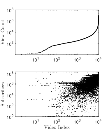
Figure 1: The top figure shows the view count of all videos (arranged according to increasing order of view count) after 14 days of the video being posted. The bottom figure shows the associated subscriber count when the video was posted.

2.1 Extreme Learning Machine

The dataset of features (described in Sec. 2.3) and view count are denoted as $\mathcal{D}=\{(x_{i},v_{i})\}_{i=1}^{N}$ where $x_{i}\in\mathds{R}^{m}$ is the feature vector, of dimension $m$, for video $i$, and $v_{i}$ is the total view count for video $i$. Here, $N$ is the number of videos in the training dataset (The ELM was trained for three categories of videos, for details see Sec. 2.3). The ELM is a single hidden-layer feed-forward neural network–that is, the ELM consists of an input layer, a single hidden layer of $L$ neurons and an output layer. Each hidden-layer neuron can have a unique transfer function. Popular transfer functions include the sigmoid, hyperbolic tangent, and Gaussian. However any non-linear piecewise continuous function can be utilized. The output layer is obtained by a weighted linear combination of the output of the $L$ hidden neurons.

The ELM model presented in [24, 25] is given by:

$$v_{i}=\sum_{k=1}^{L}\beta_{k}h_{k}(x_{i};\theta_{k}),$$ (1)

where $\beta_{k}$ is the weight of neuron $k$, and $h_{k}(\cdot;\theta_{k})$ is the hidden-layer neuron transfer function with parameter $\theta_{k}$, and $L$ is the total number of hidden-layer neurons in the ELM. Given $\mathcal{D}$, how can the ELM model parameters $\beta_{k},\theta_{k},$ and $L$ in (1) be selected? Given $L$, the ELM trains $\beta_{k}$ and $\theta_{k}$ in two steps. First, the hidden layer parameters $\theta_{k}$ are randomly initialized. Any continuous probability distribution can be used to initialize the parameters $\theta_{k}$. Second, the parameters $\beta_{k}$ are selected to minimize the square error between the model output and the measured output from $\mathcal{D}$. Formally,

$$\beta^{*}\in\underset{\beta\in\mathds{R}^{L}}{\operatorname{argmax}}\Big{\{}||H\beta-V||^{2}_{2}\Big{\}},$$ (2)

where $H$ denotes the hidden-layer output matrix with entries $H_{kj}=h_{k}(x_{j};\theta_{k})$ for $k\in\{1,2,\dots,L\}$ and $j\in\{1,2\dots,N\}$, and $V$ the target output with entries $V=[v_{1},v_{2},\dots,v_{N}]$. The solution to (2) is given by $\beta^{*}=H^{\dagger}V$ where $H^{\dagger}$ denotes the Moore-Penrose generalized inverse of $H$. The major benefit of using the ELM, compared to other single layer feed-forward neural network, is that the training only requires the random generation of the parameters $\theta_{k}$, and the parameters $\beta_{k}$ can be computed as the solution of a set of linear equations. The computational cost of training the ELM is $O(N^{3})$ for constructing the Moore-Penrose inverse [26].

2.2 Sensitivity Analysis (Background)

There are several sensitivity analysis techniques available in the literature [27, 28] which can be classified into two groups: filter methods, and wrapper methods. The filter methods consider only the meta-level features and the viewcount without the information available from a machine learning algorithm. The wrapper methods, on the other hand, utilize the information from the machine learning algorithm. Typically, wrapper methods give a more accurate measure of the sensitivity compared to filter methods [27, 28]. However, filter methods are computationally less expensive than wrapper methods and do not require the training and evaluation of the machine learning algorithm. Given the noise present in the meta-level features (Fig. 1) and the non-linearity between the meta-level features and view count , filter methods are not suitable for the sensitivity analysis of the meta-level features. Hence, in this section we focus on two wrapper methods suitable for estimating the sensitivity of meta-level features on the view count of YouTube videos.

For the first method we focus on the ELM (1) for evaluating the sensitivity of the meta-level features, however the method can be used for any machine learning method. Given that the ELM (1) is a single feed-forward hidden layer neural network, it is possible to evaluate the sensitivity of the meta-level features by taking the partial derivative of (1) for the trained ELM. Note that this method is utilized to estimate the sensitivity of input features in neural networks [29]. The sum of squares derivatives, denoted by $\text{SSD}_{k}$ for meta-level feature $x(k)$, is given by:

$$\text{SSD}_{k} =\sum_{i=1}^{N}\Big{(}\frac{\partial v_{i}}{\partial x(k)}\Big{)}^{2}=\sum_{i=1}^{N}\Big{(}\sum_{k=1}^{L}\beta_{k}\frac{\partial h_{k}(x_{i};\theta_{k})}{\partial x(k)}\Big{)}^{2}.$$ (3)

The variable with the largest $\text{SSD}_{k}$ is most influential to the prediction of the view count using the ELM $v$ (1). Note that since the ELM is trained using all the meta-level features, the $\text{SSD}_{k}$ evaluates the average sensitivity of changes in a single meta-level feature with all other features held constant.

To account for significant interdependency relationships between meta-level features requires sophisticated methods to evaluate the meta-level feature sensitivities. A state-of-the art method which can be used for this task is the Hilbert-Schmidt Independence Criterion Lasso (HSIC-Lasso) [23]. The main idea of this method is to use the benefits of least absolute shrinkage and selection operator (Lasso) with a feature wise kernel to capture the non-linear input-output dependency. A measure of the importance of a meta-level feature is then given by the coefficient of the centered Gram matrix used in the HSIC-Lasso.

Both of these methods will be applied to the YouTube dataset to study the sensitivity of the meta-level features of YouTube videos on the videos view count .

2.3 Sensitivity of YouTube Meta-Level Features and Predicting View Count

In this section, the ELM (1) and other state-of-the art machine learning methods are applied to the YouTube dataset to compute the sensitivity of a videos meta-level features on the view count of the video based on the feature importance measure $\text{SSD}_{k}$ (3). Videos of different popularity, (i.e. highly popular, popular, and unpopular as defined in Table VII in the Appendix), may have different sensitivities to the meta-level features. Hence, in this paper, we independently perform the sensitivity analysis on the three popularity categories. First we define the meta-level features for each video, then evaluate the meta-level feature sensitivities on the associated view count , and finally provide methods to predict the view count of YouTube videos using various machine learning techniques. The analysis provides insight into which meta-level features are useful for optimizing the view count of a YouTube video.

2.3.1 Meta-Level Feature Construction

Each YouTube video contains four primary components: the Thumbnail of the video, the Title of the video, the Keywords (also known as tags), and the description of the video. However, in typical user searches only a subset of the description is provided to the user. Therefore, we do not consider the contents of the description to significantly affect the view count of the video. The meta-level features are constructed using the Thumbnail, Title, and Keywords. For the Thumbnail, 19 meta-level features are computed which include: the blurriness (e.g. CannyEdge, Laplace Frequency), brightness, contrast (e.g. tone), overexposure, and entropy of the thumbnail. For the Title, 23 meta-level features are computed which include: word count, punctuation count, character count, Google hits (e.g. if the title is entered into the Google search engine how many results are found), and the Sentiment/Subjectivity of the title computed using Vader [30], and TextBlob . For the Keywords, 7 meta-level features are computed which include: the number of keywords, and keyword length. In addition, to the above 49 meta-level features, we also include auxiliary user meta-level features including: the number of subscribers, resolution of the thumbnail used, category of the video, the length of the video, and the first day view count of the video. Note that our analysis does not consider the video or audio quality of the YouTube video. Our analysis is focused on the sensitivity of the view count based on the Thumbnail, Title, Keywords, and auxiliary channel information of the user that uploaded the video. In total $54$ meta-level features are computed for each video. The complete dataset used for the sensitivity analysis is given by $\mathcal{D}=\{(x_{i},v_{i})\}_{i=1}^{N}$, with $x_{i}\in\mathds{R}^{54}$ the computed meta-level features for video $i\in\{1,\dots,N\}$, $v_{i}$ the view count 14 days after the video is published, and $N=10^{4}$, the total number of videos used for the sensitivity analysis. Note that the view count $v_{i}$ is on the log scale (i.e. if a video has $10^{6}$ views then $v_{i}=6$). This is a necessary step as the range of view counts is from $10^{2}$ to above $10^{7}$.

Prior to performing any analysis we pre-process the meta-level features in the dataset $\mathcal{D}$. First, all the meta-level features are scaled to satisfy $x(k)\in[0,1]$. Note that the meta-level features were not whitened (e.g. the meta-level data as not transformed to have an identity covariance matrix). The second pre-processing step involves removing redundant features in $\mathcal{D}$. Feature selection is a popular method for eliminating redundant meta-level features. In this paper we employ a correlation based feature selection based on the Pearson correlation coefficient (which was used for feature selection in [31]) to eliminate the redundant meta-level features. Of the original 54 meta-level features, $m=29$ meta-level features remain after the removal of the correlated meta-level features. Note that removal of these features does not significantly impact the performance of the machine learning algorithms or the sensitivity analysis results.

2.3.2 Meta-Level Feature Sensitivity

Given the dataset $\mathcal{D}=\{(x_{i},v_{i})\}_{i=1}^{N}$ constructed in Sec.2.3.1, the goal is to estimate which features significantly contribute to the view count of a video. To perform this sensitivity analysis five machine learning algorithms which include: the ELM, Bagged MARS using gCV Pruning [21], Conditional Inference Random Forest (CIRF) [18], Feed-Forward Neural Network (FFNN) [12], and the feature selection method Hilbert-Schmidt Independence Criterion Lasso (HSIC-Lasso) [23]. Each of these models is trained using a 10-fold cross validation technique, and the design parameters of each was optimized via extensive empirical evaluation. We selected the ELM (1) to contain $L=100$ neurons which ensures that we have sufficient accuracy on the predicted view count given the features $x_{i}$, while reducing the effects of over-fitting. For the CIRF the design parameter for randomly selected predictors was set to 6, and the FFNN we have 10 neurons in the hidden-layer. The HSIC-Lasso regularization parameter was set to 100. Given the trained models, the sensitivity of the view count on the meta-level features of a video is computed by evaluating the sum of squares derivatives, $\text{SSD}_{k}$ (3). Fig. 2 shows the normalized $\text{SSD}_{k}$ for the five highest sensitivity meta-level features of these five machine learning methods. Note that for the HSIC-Lasso we do not use the $\text{SSD}_{k}$ but instead the values of the coefficient of the centered Gram matrix computed from k${}^{\text{th}}$ feature which provides an estimate of the feature sensitivity. Recall, from Sec. 2.2, that larger the $\text{SSD}_{k}$ value or higher the coefficient of the centered Gram matrix the more sensitive the view count is to variations in the meta-level feature. From Fig. 2, the meta-level features with the highest sensitivities are: first day view count , number of subscribers, contrast of the video thumbnail, Google hits, number of keywords, video category, title length, and number of upper-case letters in the title respectively. Notice that all these methods have the first day view count and number of subscribers as the most sensitive meta-level features as expected. The FFNN and Bagged MARS however do not have the contrast of the video thumbnail as the third most sensitive meta-level feature compared with the other algorithms. This results as the learning method and learning rate of each of these algorithms is different which results in differences in the meta-level feature sensitivity. However as we can see from Fig. 2, the view count of a video is dependent on these eight meta-level features with the first day view count and number of subscribers being the most sensitive features.

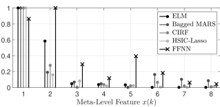
Figure 2: Sensitivity of the meta-level features computed using the sum of squares derivatives $\text{SSD}_{k}$ (3) for the ELM, Bagged MARS, CIRF, and FFN, and the associated coefficient of the centered Gram matrix for the HSIC-Lasso using the dataset $\mathcal{D}$ defined in Sec.2.3.1. The meta-level features k=1 to k=8 are associated with: first day view count , number of subscribers, contrast of the video thumbnail, Google hits, number of keywords, video category, title length, and number of upper-case letters in the title respectively. Similar results are obtained for highly popular, popular, and unpopular videos as defined in Table VII.

As expected, Fig. 2 shows that if the first day view count is high then the associated view count 14 days after the video is posted will be high. Additionally, if there is a large number of subscribers to the channel that posted the video, then the associated view count after 14 days is also expected to be large. As expected, the properties of the title and keywords also contribute to the view count of the video however with less sensitivity then the thumbnail of the video. Therefore, to increase the view count of a video it is vital to increase the number of subscribers, and focus on the quality of the Thumbnail used. A surprising result is that the sensitivity of the view count resulting from changes in these meta-level features are negligible across the three popularity classes of videos (i.e. highly popular, popular, and unpopular as defined in Table VII). Therefore, regardless of the expected popularity of a video, a channel owner should focus on maximizing the number of subscribers and the quality of the thumbnail to increase the associated view count of a video.

2.3.3 Predicting the view count of YouTube videos

In this section we illustrate how machine learning methods can be used to the view count of a YouTube video. The machine learning methods used for prediction include: the Extreme Learning Machine (1), Feed-Forward Neural Network [12], Stacked Auto-Encoder Deep Neural-Network [13, 14], Elasticnet [15], Lasso, Relaxed Lasso [16], Quantile Regression with Lasso [17], Conditional Inference Random Forest [18], Boosted Generalized Additive Model [19, 20], Bagged MARS using gCV Pruning [21], Generalized Linear Model with Stepwise Feature Selection using Akaike information criterion, and Spike and Slab Regression [22]. For each method their predictive performance and the top-five highest sensitivity meta-level features are provided.

To perform the analysis we train each model using an identical 10-fold cross validation method with the dataset $\mathcal{D}=\{(x_{i},v_{i})\}_{i=1}^{N}$ with all the meta-level features included. The predictive performance of the machine learning methods are evaluated using the root-mean-square error (RMSE) and the R² (e.g. coefficient of determination). Note that for both training and evaluation the view count is pre-processed to be on the log scale (i.e. if the view count is $10^{6}$, the associated label is $v_{i}=6$).

The predictive performance and the top-five highest sensitivity meta-level features of the machine learning methods are provided in Table I. In Table I the meta-level feature numbers are identical to those defined in Fig. 2. As seen from Table I, the ELM has the lowest RMSE of 0.44 which is comparable to the RMSE of the Conditional Inference Random Forest and Feed-Forward Neural Network which have 0.47 and 0.48 respectively. The R² of the ELM, Feed-Forward Neural Network and Conditional Inference Random Forest are also comparable with values of 0.77, 0.79, and 0.80. Therefore any of these methods could be used to estimate the view count of a YouTube video. A key question is which of the meta-level features $x(k)$ are most sensitive between these machine learning methods. As seen from the results in Table I the top two most important features are the first day view count and the number of subscribers, and the majority of methods suggest that the number of Google hits is also an important meta-level feature. Interestingly the Conditional Inference Random Forest, Boosted Generalized Additive Model, and the Bagged MARS using gCV Pruning do not consider the number of Google hits in the top five most sensitive features and instead use the video category. This is consistent with the result that videos in the “Music” category are the most viewed on YouTube, followed by “Entertainment” and “People and Blogs”. Only the Bagged MARS using gCV Pruning considers the meta-level features of title length and number of upper-case letters in the title to be in the five most sensitive features compared with the other machine learning methods. This result suggests that the number of Google hits associated with the title significantly contributes to the video’s popularity however the view count is not very sensitive to the specific length and number of upper-case letters in the title. Therefore, when performing meta-level feature optimization for a video a user should focus on the meta-level features of: first day view count , number of subscribers, contrast of the video thumbnail, Google hits, number of keywords, and video category.

TABLE I: Performance and Feature Sensitivity

Method	RMSE	R2	Features $x(k)$
Extreme Learning Machine	0.44	0.77	1	2	3	4	5
Feed-Forward Neural Network	0.48	0.79	2	1	5	3	6
Stacked Auto-Encoder DNN	0.59	0.66	1	2	3	4	5
Elasticnet	0.57	0.64	1	2	3	4	5
Lasso	0.53	0.66	1	2	3	4	5
Relaxed Lasso	1.14	0.64	1	2	3	4	5
Quantile Regression with Lasso	0.60	0.62	1	2	3	4	5
CI Random Forest	0.47	0.80	1	2	6	4	5
Boosted GAM	0.50	0.77	1	2	6	4	5
Bagged MARS	0.50	0.77	1	2	6	7	8
GLM with Feature Selection	0.53	0.67	1	2	3	4	5
Spike and Slab Regression	0.53	0.67	1	2	3	4	5

To estimate the view count of an unpublished video (a video that is about to be posted for the first time) we can not utilize the most sensitive meta-level feature of the machine learning algorithms which is the first day view count . Is it still possible to estimate the view count with the remaining meta-level features? To answer this question we compare the performance of the ELM using the 28 meta-level features with the view count on the first day removed. Fig. 3 shows the predicted view count of the ELM trained using 29 meta-level features, and Fig. 3 shows the predicted view count using the 28 meta-level features. As expected, Fig. 3 illustrates that the predictive accuracy of the ELM decreases if the view count on the first day is removed. Though there is a drop in the predictive accuracy of the ELM trained using the 28 meta-level features, it still contains sufficient predictive accuracy to aid in the selection of the meta-level features to increase the view count of a video. Note that similar performance results are obtained for the Feed-Forward Neural Network and Conditional Inference Random Forest when performing the prediction with the first day view count removed. Therefore these prediction methods can be used to optimize the meta-level features of unpublished videos where the optimization can focus on the meta-level features of: number of subscribers, contrast of the video thumbnail, Google hits, number of keywords, and video category.

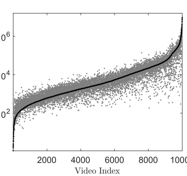
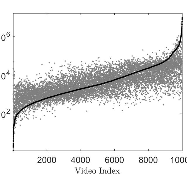
Figure 3: Predictive view count using an ELM with the actual view count (black dots) and predicted view count indicated by the (gray dots). Fig. 3 illustrates the results for a trained ELM (1) using all 29 meta-level features defined in Sec. 2.3. Fig. 3 illustrates the results for a trained ELM (1) using the 28 meta-level features (first day view count removed from the 29 meta-level features defined in Sec. 2.3).

2.4 Sensitivity to meta-level optimization

Sec. 2.3, described how meta-level features (e.g. number of subscribers) can be used to estimate the popularity of a video. In this section, we analyze how changing meta-level features, after a video is posted, impacts the user engagement of the video. Meta-level data plays a significant role in the discovery of content, through YouTube search, and in video recommendation, through the YouTube related videos. Hence, “optimizing” the meta-level data to enhance the discoverability and user engagement of videos is of significant importance to content providers. Therefore, in this section, we study how optimizing the title, thumbnail or keywords affect the view count of YouTube videos.

To perform the analysis we utilize the dataset (see Table VIII in the Appendix), and remove any time-sensitive videos. Time-sensitive videos are those videos that are relevant for a short period of time and the popularity of such videos cannot be improved by optimization. We removed the following two time-sensitive categories of videos: “politics” and “movies and trailers”. In addition, we removed videos (from other categories) which contained the following keywords in their video meta-data: “holiday”, “movie”, or “trailers”. For example, holiday videos are not watched frequently during off-holiday times.

Let $\hat{\tau}_{i}$ be the time at which the meta-level optimization was performed on video $i$ and let $s_{i}$, denote the corresponding sensitivity. We characterize the sensitivity to meta-level optimization as follows:

$$s_{i}=\frac{\left(\sum_{t=\hat{\tau}_{i}}^{\hat{\tau}_{i}+6}v_{i}(t)\right)/7}{\left(\sum_{t=\hat{\tau}_{i}-6}^{\hat{\tau}_{i}}v_{i}(t)\right)/7}$$ (4)

The numerator of (4) is the mean value of the view count $7$ days after optimization. Similarly, the denominator of (4) is the mean value of the view count $7$ days before optimization. The results are provided in Table II for optimization of the title, thumbnail, and keywords.

Optimization	Fraction of Videos with increased popularity
Title change	0.52
Thumbnail change	0.533
Keyword change	0.50
No change	0.35

TABLE II: Sensitivity to Meta-Level Optimization. The table shows than in more than $50\%$ the videos, meta-level optimization resulted in an increase in the popularity of the video.

As shown in Table II, at least half of the optimizations resulted in an increase in the popularity of the video. In addition, compared to videos with no optimization, the meta-level optimization improves the probability of increased popularity by $45\%$. This is consistent with YouTube and BBTV recommendation to optimize meta-level features to increase user engagement. However, some class of videos benefit from optimizing meta-data much more than others. The effect may be due to small user channels, which have limited number of videos and subscribers, gain by optimizing the meta-level data of the video compared to hugely popular channels such as Sony or CNN. The highly popular channel (e.g. Sony or CNN) upload videos frequently (even multiple times daily), so video content becomes irrelevant quickly. The question of which class of users gain by optimizing the meta level features of the video is part of our ongoing research.

Table III summarizes the impact of various meta-level changes on the three major sources of YouTube traffic, i.e. YouTube search, YouTube promoted and traffic from related videos. For those videos where meta-level optimization increased the popularity (the ratio of the mean value of the views after and before optimization is higher than one), we computed the sensitivity for various traffic sources as in (4). Table III summarizes the median statistics of the ratio of the traffic sources before and after optimization.

Optimization	Related	Promoted	Search
Title change	$1.13$	NA	$\mathbf{1.24}$
Thumbnail change	$\mathbf{1.20}$	NA10	$1.125$
Keyword change	$\mathbf{1.10}$	$\mathbf{1.16}$	$1$

TABLE III: Sensitivity of various traffic sources to meta-level optimization, for videos with increased popularity. The title optimization resulted in significant improvement (approximately $25\%$) from the YouTube search. Similarly, thumbnail optimization improved traffic from the related videos and keyword optimization resulted in increased traffic from related and promoted videos.

The title optimization resulted in significant improvement (approximately $25\%$) from the YouTube search. Similarly, thumbnail optimization improved traffic from the related videos and keyword optimization resulted in increased traffic from related and promoted videos.

Summary: This section studied the sensitivity of view count with respect to meta-level optimization. The main finding is that meta-level optimization increased the popularity of video in the majority of cases. In addition, we found that optimizing the title improved traffic from YouTube search. Similarly, thumbnail optimization improved traffic from the related videos and keyword optimization resulted in increased traffic from related and promoted videos.

3 Social interaction of the channel with YouTube users

In this section, we use time series analysis methods to determine how the social interaction of a YouTube channel with its viewers affects the view count dynamics. This section is organized as follows. Sec. 3.1, characterizes the causal relationship between the subscribers and view count of a channel using Granger causality test. In Sec. 3.2, we investigate how the popularity of the channel is affected by the scheduling dynamics of the channel. When channels deviate from a regular upload schedule, the view count and the comment count of the channel increase. In Sec. 3.3, we address the problem of separating the view count dynamics due to virality (viewcount resulting from subscribers) and migration (views from non-subscribers) and exogenous events using a generalized Gompertz model. Finally, Sec. 3.4, we studies the effect of video playlists on the view count. The main conclusion outlined in Sec. 3.4 is that the dynamics of the view count in a playlist is highly correlated and the effects of “migration” causes the view count of videos to decrease even with an increase in the subscriber count.

3.1 Causality between subscribers and view count in YouTube

In this section the goal is to detect the causal relationship between subscriber and viewer counts and how it can be used to estimate the next day subscriber count of a channel. The results are of interest for measuring the popularity of a YouTube channel. Fig. 4 displays the subscriber and view count dynamics of a popular movie trailer channel in YouTube. It is clear from Fig. 4 that the subscribers “spike” with a corresponding “spike” in the view count. In this section we model this causal relationship of the subscribers and view count using the Granger causality test from the econometric literature [32].

The main idea of Granger causality is that if the value(s) of a lagged time-series can be used to predict another time-series, then the lagged time-series is said to “Granger cause” the predicted time-series. To formalize the Granger causality model, let $s^{j}(t)$ denote the number of subscribers to a channel $j$ on day $t$, and $v_{i}^{j}(t)$ the corresponding view count for a video $i$ on channel $j$ on day $t$. The total number of videos in a channel on day $t$ is denoted by $\mathcal{I}(t)$. Define,

$$\hat{v}^{j}(t)=\sum_{i=1}^{\mathcal{I}(t)}v_{i}^{j}(t),$$ (5)

as the total view count of channel $j$ at time $t$. The Granger causality test involves testing if the coefficients $b_{i}$ are non-zero in the following equation which models the relationship between subscribers and view counts:

$$s^{j}(t)=\sum_{k=1}^{n_{s}}a_{k}^{j}s^{j}(t-k)+\sum_{i=k}^{n_{v}}b_{k}^{j}\hat{v}^{j}(t-k)+\varepsilon^{j}(t),$$ (6)

where $\varepsilon^{j}(t)$ represents normal white noise for channel $j$ at time $t$. The parameters $\{a_{i}^{j}\}_{\{i=1,\dots,n_{s}\}}$ and $\{b_{i}^{j}\}_{\{i=1,\dots,n_{v}\}}$ are the coefficients of the AR model in (6) for channel $j$, with $n_{s}$ and $n_{v}$ denoting the lags for the subscriber and view counts time series respectively. If the time-series $\mathcal{D}^{j}=\{s^{j}(t),\hat{v}^{j}(t)\}_{t\in\{1,\dots,T\}}$ of a channel $j$ fits the model (6), then we can test for a causal relationship between subscribers and view count. In equation (6), it is assumed that $|a_{i}|<1$, $|b_{i}|<1$ for stationarity. The causal relationship can be formulated as a hypothesis testing problem as follows:

$$H_{0}:b_{1}=\dots=b_{n_{v}}=0\text{ vs. }H_{1}:\text{Atleast one }b_{i}\neq 0.$$ (7)

The rejection of the null hypothesis, $H_{0}$, implies that there is a causal relationship between subscriber and view counts.

First, we use Box-Ljung test [33] is to evaluate the quality of the model (6) for the given dataset $\mathcal{D}^{j}$. If satisfied, then the Granger causality hypothesis (7) is evaluated using the Wald test [34]. If both hypothesis tests pass then we can conclude that the time series $\mathcal{D}^{j}$ satisfies Granger causality–that is, the previous day subscriber and view count have a causal relationship with the current subscriber count.

A key question prior to performing the Granger causality test is what percentage of videos in the YouTube dataset (Appendix) satisfy the AR model in (6). To perform this analysis we apply the Box-Ljung test with a confidence of 0.95 (p-value = $0.05$). First, we need to select $n_{s}$ and $n_{v}$, the number of lags for the subscribers and view count time series. For $n_{s}=n_{v}=1$, we found that only $20\%$ of the channels satisfy the model (6). When $n_{s}$ and $n_{v}$ are increased to $2$, the number of channels satisfying the model increases to $63\%$. For $n_{s}=n_{v}=3$, we found that $91\%$ of the channels satisfy the model (6), with a confidence of $0.95$ (p-value = $0.05$). Hence, in the below analysis we select $n_{s}=n_{v}=3$. It is interesting to note that the mean value of coefficients $b_{i}$ decrease as $i$ increases indicating that older view counts have less influence on the subscriber count. Similar results also hold for the coefficients $a_{i}$. Hence, as expected, the previous day subscriber count and the previous day view count most influence the current subscriber count.

The next key question is does their exist a causal relationship between the subscriber dynamics and the view count dynamics. This is modeled using the hypothesis in (7). To test (7) we use the Wald test with a confidence of $0.95$ (p-value = $0.05$) and found that approximately $55\%$ of the channels satisfy the hypothesis. For approximately $55\%$ of the channels that satisfy the AR model (6), the view count “Granger causes” the current subscriber count. Interestingly, if different channel categories are accounted for then the percentage of channels that satisfy Granger causality vary widely as illustrated in Table IV. For example, $80\%$ of the Entertainment channels satisfy Granger causality while only $40\%$ of the Food channels satisfy Granger causality. These results illustrate the importance of channel owners to not only maximize their subscriber count, but to also upload new videos or increase the views of old videos to increase their channels popularity (i.e. via increasing their subscriber count). Additionally, from our analysis in Sec.2 which illustrates that the view count of a posted video is sensitive to the number of subscribers of the channel, increasing the number of subscribers will also increase the view count of videos that are uploaded by the channel owners.

Category	Fraction
Gaming	0.60
Entertainment	0.80
Food	0.40
Sports	0.67

TABLE IV: Fraction of channels satisfying the hypothesis: View count “Granger causes” subscriber count, split according to category.

Figure 4: Viewcount and subscribers for the popular movie trailer channel: VISOTrailers. The Granger causality test for view counts “Granger causes” subscriber count is true with a p-value of $5\times 10^{-8}$.

3.2 Scheduling dynamics in YouTube

In this section, we investigate the scheduling dynamics of YouTube channels. We find the interesting property that for popular gaming YouTube channels with a dominant upload schedule, deviating from the schedule increases the views and the comment counts of the channel.

Creator Academy in their best practice section recommends to upload videos on a regular schedule to get repeat views. The reason for a regular upload schedule is to increase the user engagement and to rank higher in the YouTube recommendation list. However, we show in this section that going “off the schedule” can be beneficial for a gaming YouTube channel, with a regular upload schedule, in terms of the number of views and the number of comments.

From the dataset, we ‘filtered out’ video channels with a dominant upload schedule, as follows: The dominant upload schedule was identified by taking the periodogram of the upload times of the channel and then comparing the highest value to the next highest value. If the ratio defined above is greater than $2$, we say that the channel has a dominant upload schedule. From the dataset containing $25$ thousand channels, only $6500$ channels contain a dominant upload schedule. Some channels, particularly those that contain high amounts of copied videos such as trailers, movie/TV snippets upload videos on a daily basis. These have been removed from the above analysis. The expectation is that by doing so we concentrate on those channels that contain only user generated content.

We found that channels with gaming content account for $75\%$ of the $6500$ channels with a dominant upload schedule and the main tags associated with the videos were: “game”, “gameplay” and “videogame”. We computed the average views when the channel goes off the schedule and found that on an average when the channel goes off schedule the channel gains views $97\%$ of the time and the channel gains comments $68\%$ of the time. This suggests that channels with “gameplay” content have periodic upload schedule and benefit from going off the schedule.

3.3 Modeling the View count Dynamics of Videos with Exogenous Events

Several time-series analysis methods have been employed in the literature to model the view count dynamics of YouTube videos. These include ARMA time series models [1], multivariate linear regression models [2], hidden Markov models [35], normal distribution fitting [36], and parametric model fitting [3, 4]. Though all these models provide an estimate of the view count dynamics of videos, we are interested in segmenting view count dynamics of a video resulting from subscribers, non-subscribers and exogenous events. Exogenous events are due to video promotion on other social networking platform such as Facebook or the video being referenced by a popular news organization or celebrity on Twitter. This is motivated by two reasons. First, removing view count dynamics due to exogenous events provides an accurate estimate of sensitivity of meta-level features in Sec. 2. Second, extracting the view count resulting from exogenous events gives an estimate of the efficiency of video promotion.

The view count dynamics of popular videos in YouTube typically show an initial viral behaviour, due to subscribers watching the content, and then a linear growth resulting from non-subscribers. The linear growth is due to new users migrating from other channels or due to interested users discovering the content either through search or recommendations (we call this phenomenon migration similar to [3]). Hence, without exogenous events, the view count dynamics of a video due to subscribers and non-subscribers can be estimated using piecewise linear and non-linear segments. In [3], it is shown that a Gompertz time series model can be modeled the view count dynamics from subscribers and non-subscribers, if no exogenous events are present. In this paper, we generalize the model in [3] to account for views from exogenous events. It should be noted that classical change-point detection methods [37] cannot be used here as the underlying distribution generating the view count is unknown.

To account for the view count dynamics introduced from exogenous events we use the generalized Gompertz model given by:

$$\begin{aligned} \bar{v}_{i}(t)&=\sum_{k=0}^{K_{\text{max}}}w^{k}_{i}(t)u(t-t_{k}),\\ w_{i}^{k}(t)&=M_{k}\left(1-e^{-\eta_{k}\left(e^{b_{k}\left(t-t_{k}\right)}-1\right)}\right)+c_{k}(t-t_{k}),\end{aligned}$$ (8)

where $\bar{v}_{i}(t)$ is the total view count for video $i$ at time $t$, $u(\cdot)$ is the unit step function, $t_{0}$ is the time the video was uploaded, $t_{k}$ with $k\in\{1,\dots,K_{\text{max}}\}$ are the times associated with the $K_{\text{max}}$ exogenous events, and $w^{k}_{i}(t)$ are Gompertz models which account for the view count dynamics from uploading the video and from the exogenous events. In total there are $K_{\text{max}}+1$ Gompertz models with each having parameters $t_{k},M_{k},\eta_{k},b_{k}$. $M_{k}$ is the maximum number of requests not including migration for an exogenous event at $t_{k}$, $\eta_{k}$ and $b_{k}$ model the initial growth dynamics from event $t_{k}$, and $c_{k}$ accounts for the migration of other users to the video. In (8) the parameters $\{M_{k},\eta_{k},b_{k}\}_{k=0}$ are associated with the subscriber views when the video is initially posted, the parameters $\{t_{k},M_{k},\eta_{k},b_{k}\}_{k=1}^{K_{\text{max}}}$ are associated with views introduced from exogenous events, and the views introduced from migration are given by $\{c_{k}\}_{k=0}^{K_{\text{max}}}$. Each Gompertz model (8) captures the initial viral growth when the video is initially available to users, followed by a linearly increasing growth resulting from user migration to the video.

The parameters $\theta_{i}=\{a_{k},t_{k},M_{k},\eta_{k},b_{k},c_{k}\}_{k=0}^{K_{\text{max}}}$ in (8) can be estimated by solving the following mixed-integer non-linear program:

$$\theta_{i} \in\operatorname{arg\ min}\Big{\{}\sum_{t=0}^{T_{i}}\big{(}\bar{v}_{i}(t)-v_{i}(t)\big{)}^{2}+\lambda K\Big{\}}$$

$$K=\sum_{k=0}^{K_{\text{max}}}a_{k},\quad\quad a_{k}\in\{0,1\}\quad\quad k\in\{0,\dots,K_{\text{max}}\},$$ (9)

with $T_{i}$ the time index of the last recorded views of video $v_{i}$, and $a_{k}$ a binary variable equal to $1$ if an exogenous event is present at $t_{k}$. Note that (9) is a difficult optimization problem as the objective is non-convex as a result of the binary variables $a_{k}$ [38]. In the YouTube social network when an exogenous event occurs this causes a large and sudden increase in the number of views, however as seen in Fig. 5, a few days after the exogenous event occurs the views only result from migration (i.e. linear increase in total views). Assuming that each exogenous event is followed by a linear increase in views we can estimate the total number of exogenous events $K_{\text{max}}$ present in a given time-series by first using a segmented linear regression method, and then counting the number of segments of connected linear segments with a slope less then $c_{\text{max}}$. The parameter $c_{\text{max}}$ is the maximum slope for the views to be considered to result from viewer migration. Plugging $K_{\text{max}}$ into (9) results in the optimization of a non-linear program for the unknowns $\{t_{k},M_{k},\eta_{k},b_{k},c_{k}\}_{k=0}^{K_{\text{max}}}$. This optimization problem can be solved using sequential quadratic programming techniques [39].

To illustrate how the Gompertz model (8) can be used to detect for exogenous events, we apply (8) to the view count dynamics of a video that only contains a single exogenous event. Fig. 5 displays the total view count of a video where an exogenous event occurs at time $t=41$ (i.e. $t_{1}=41$ in (8)) days after the video is posted. The initial increase in views for the video for $t\leq 7$ days results from the $2910$ subscribers of the channel viewing the video. For $7\leq t\leq 41$, other users that are not subscribed to the channel migrate to view the video at an approximately constant rate of $13$ views/day. At $t=41$, an exogenous event occurs causing an increase in the views per day. The difference in viewers, resulting from the exogenous event, is $7174$. For $t\geq 43$, the views result primarily from the migration of users to approximately $2$ views/day. Hence, using the generalized Gompertz model (8) we can differentiate between subscriber views, views caused by exogenous events, and views caused by migration.

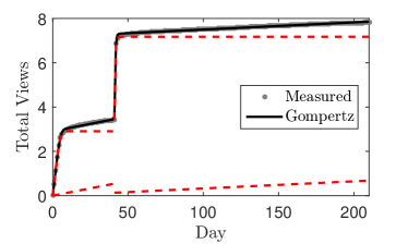
Figure 5: Due to an exogenous event on day $41$, there is a sudden increase in the number of views. The total view count fitted by the Gompertz model $\bar{v}_{i}(t)$ in (8) is shown in black with the virality (exponential) and migration (linear) illustrated by the dotted red.

3.4 Video Playthrough Dynamics

One of the most popular sequences of YouTube videos is the video game “playthrough”. A video game playthrough is a set of videos for which each video has a relaxed and casual focus on the game that is being played and typically contains commentary from the user presenting the playthrough. Unlike YouTube channels such as CNN, BBC, and CBC in which each new video can be considered independent from the others, in a video playthrough the future view count of videos are influenced by the previously posted videos in the playthrough. To illustrate this effect we consider a video playthrough for the game “BioShock Infinite”–a popular video game released in 2013. The channel, popular for hosting such video playthroughs, contains close to $4500$ videos and $180$ video playthroughs. The channel is highly popular and has garnered a combined view count close to $100$ million views with $150$ thousand subscribers over a period of $3$ years. Fig. 6 illustrates that the early view count dynamics are highly correlated with the view count dynamics of future videos. Both the short term view count and long term migration of future videos in the playthrough decrease after the initial video in the playthrough is posted. This results for two reasons, either the viewers purchase the game, or the viewers leave as the subsequent playthroughs become repetitive as a result of game quality or video commentary quality. A unique effect with video playthroughs is that though the number of subscribers to the channel hosting the videos in Fig. 6 increases over the 600 day period, the linear migration is still maintained after the initial 50 days after the playthrough is published. Additionally, the slope of the migration is related to the early total view count as illustrated in Fig. 6(b).

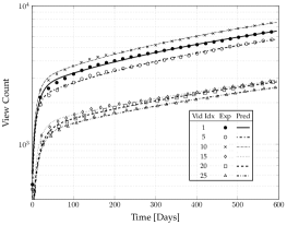
(a) Actual and predicted view count of playthrough. We plot the 1, 5, 10, 15, 20 and 25 video from the playlist containing $25$ videos. In the legend, Exp and Pred corresponds to the actual and the predicted value using (8), respectively. Figure shows that the view counts decreases for subsequent videos in the playlist.

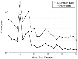
(b) The virality rate specifies the early views due to subscribers, and the migration rate (in units of views/1000 days) specifies the subsequent linear growth due to non-subscribers.

Figure 6: Actual and predicted view count of a playthrough containing 25 YouTube videos for the game “BioShock Infinite”. The predictions are computed by fitting a modified Gompertz model (8) to the measured view count for each video in the playthrough.

4 Conclusion

In this paper, we conducted a data-driven study of YouTube based on a large dataset (see Appendix for details). First, by using several machine learning methods, we investigated the sensitivity of the videos meta-level features on the view counts of videos. It was found that the most important meta-level features include: first day view count , number of subscribers, contrast of the video thumbnail, Google hits, number of keywords, video category, title length, and number of upper-case letters in the title respectively. Additionally, optimizing the meta-data after the video is posted improves the popularity of the video. The social dynamics (the interaction of the channel) also affects the popularity of the channel. Using the Granger causality test, we showed that the view count has a casual effect on the subscriber count of the channel. A generalized Gompertz model was also presented which can allow the classification of a videos view count dynamics which results from subscribers, migration, and exogenous events. This is an important model as it allows the views to be categorized as resulting from the video or from exogenous events which bring viewers to the video. The final result of the paper was to study the upload scheduling dynamics of gaming channels in YouTube. It was found that going “off schedule” can actually increase the popularity of a channel. Our conclusions are based on the BBTV dataset. Extrapolating these results to other YouTube datasets is an important problem worth addressing in future work. Another extension of the current work could involve studying the effect of video characteristics on different traffic sources, for example the affect of tweets or posts of videos on Twitter or Facebook.

Description of YouTube Dataset

This paper uses the dataset provided by BBTV. The dataset contains daily samples of metadata of YouTube videos on the BBTV platform from April, 2007 to May, 2015, and has a size of around $200$ gigabytes. The dataset contains around $6$ million videos spread over $25$ thousand channels. Table V shows the statistics summary of the videos present in the dataset.

TABLE V: Dataset summary

Videos	$6$ million
Channels	$26$ thousand
Average number of videos (per channel)	250
Average age of videos	275 days
Average number of views (per video)	$10$ thousand

Table VI, shows the summary of the various category of the videos present in the dataset. The dataset contains a large percentage of gaming videos.

TABLE VI: YouTube dataset categories (out of $6$ million videos)

Category	Fraction
Gaming	0.69
Entertainment	0.07
Food	0.07
Music	0.035
Sports	0.017

Fig. 7 shows the fraction of videos as a function of the age of the videos. There is a large fraction of videos uploaded within a year. Also, the dataset captures the exponential growth in the number of videos uploaded to YouTube.

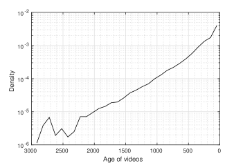
Figure 7: The fraction of videos in the dataset as a function of the age of the videos. There is a significant percentage of newer videos (videos with less age) compared to older videos. Hence, the dataset capture the exponential growth of the number of videos uploaded to YouTube.

Similar to [3], we define three categories of videos based on their popularity: Highly popular, popular, and unpopular. Table VII gives a summary of the fraction of videos in the dataset belonging to each category. As can be seen from Table VII, the majority of the videos in the dataset belong to the popular category.

TABLE VII: Popularity distribution of videos in the dataset

Criteria	Fraction
Highly Popular (Total Views $>10^{4}$)	0.12
Popular ($150<$ Total Views $<10^{4}$)	0.67
Unpopular (Total Views $<150$)	0.21

A unique feature of the dataset is that it contains information about the “meta-level optimization” for videos. The meta-level optimization is a change in the title, tags or thumbnail, of an existing video in order to increase the popularity. BBTV markets a product that intelligently automates the meta-level optimization. Table VIII gives a summary of the statistics of the various meta-level optimization present in the dataset.

TABLE VIII: Optimization summary statistics

Optimization	# Videos
Title change	$21$ thousand
Thumbnail change	$13$ thousand
Keyword change	$21$ thousand

References

- [1] G. Gürsun, M. Crovella, and I. Matta, “Describing and forecasting video access patterns,” in 2011 Proc. of INFOCOM. IEEE, 2011, pp. 16–20.
- [2] H. Pinto, J. Almeida, and M. Gonçalves, “Using early view patterns to predict the popularity of YouTube videos,” in Proc. of the sixth ACM Int. Conf. on Web search and Data mining. ACM, 2013, pp. 365–374.
- [3] C. Richier, E. Altman, R. Elazouzi, T. Jimenez, G. Linares, and Y. Portilla, “Bio-inspired models for characterizing YouTube viewcout,” in 2014 IEEE/ACM Int. Conf. on Advances in Social Networks Analysis and Mining. IEEE, 2014, pp. 297–305.
- [4] C. Richier, R. Elazouzi, T. Jimenez, E. Altman, and G. Linares, “Forecasting online contents’ popularity,” arXiv preprint arXiv:1506.00178, 2015.
- [5] A. Zhang, “Judging YouTube by its covers,” Department of Computer Science and Engineering, University of California, San Diego, Tech. Rep., 2015. [Online]. Available: http://cseweb.ucsd.edu/~jmcauley/cse255/reports/wi15/Angel%20Zhang.pdf
- [6] T. Yamasaki, S. Sano, and K. Aizawa, “Social popularity score: Predicting numbers of views, comments, and favorites of social photos using only annotations,” in Proc. of the First Int. Workshop on Internet-Scale Multimedia Management. ACM, 2014, pp. 3–8.
- [7] T. Yamasaki, J. Hu, K. Aizawa, and T. Mei, “Power of tags: Predicting popularity of social media in geo-spatial and temporal contexts,” in Advances in Multimedia Information Processing. Springer, 2015, pp. 149–158.
- [8] T. Trzcinski and P. Rokita, “Predicting popularity of online videos using support vector regression,” arXiv preprint arXiv:1510.06223, 2015.
- [9] Y. Ding, Y. Du, Y. Hu, Z. Liu, L. Wang, K. Ross, and A. Ghose, “Broadcast yourself: Understanding YouTube uploaders,” in Proc. of the ACM SIGCOMM Conf. on Internet Measurement. New York, NY, USA: ACM, 2011, pp. 361–370.
- [10] Q. He, T. Shang, F. Zhuang, and Z. Shi, “Parallel extreme learning machine for regression based on mapreduce,” Neurocomputing, vol. 102, pp. 52–58, 2013.
- [11] A. Basu, S. Shuo, H. Zhou, M. Lim, and G. Huang, “Silicon spiking neurons for hardware implementation of extreme learning machines,” Neurocomputing, vol. 102, pp. 125–134, 2013.
- [12] C. Bishop, Pattern Recognition and Machine Learning. Springer-Verlag New York, 2006.
- [13] J. Hu, J. Zhang, C. Zhang, and J. Wang, “A new deep neural network based on a stack of single-hidden-layer feedforward neural networks with randomly fixed hidden neurons,” Neurocomputing, 2015.
- [14] J. Schmidhuber, “Deep learning in neural networks: An overview,” Neural Networks, vol. 61, pp. 85–117, 2015.
- [15] H. Zou and T. Hastie, “Regularization and variable selection via the elastic net,” Journal of the Royal Statistical Society: Series B (Statistical Methodology), vol. 67, no. 2, pp. 301–320, 2005.
- [16] N. Meinshausen, “Relaxed lasso,” Computational Statistics & Data Analysis, vol. 52, no. 1, pp. 374–393, 2007.
- [17] B. Peng and L. Wang, “An iterative coordinate descent algorithm for high-dimensional nonconvex penalized quantile regression,” Journal of Computational and Graphical Statistics, vol. 24, no. 3, pp. 676–694, 2015.
- [18] T. Hothorn, K. Hornik, and A. Zeileis, “Unbiased recursive partitioning: A conditional inference framework,” Journal of Computational and Graphical statistics, vol. 15, no. 3, pp. 651–674, 2006.
- [19] W. Venables and B. Ripley, Modern applied statistics with S-PLUS. Springer Science & Business Media, 2013.
- [20] T. Hothorn, P. Bühlmann, T. Kneib, M. Schmid, and B. Hofner, “Model-based boosting 2.0,” Journal of Machine Learning Research, vol. 11, pp. 2109–2113, 2010.
- [21] H. Drucker, “Improving regressors using boosting techniques,” in ICML, vol. 97, 1997, pp. 107–115.
- [22] H. Ishwaran and S. Rao, “Spike and slab variable selection: frequentist and bayesian strategies,” Annals of Statistics, pp. 730–773, 2005.
- [23] M. Yamada, W. Jitkrittum, L. Sigal, E. Xing, and M. Sugiyama, “High-dimensional feature selection by feature-wise kernelized lasso,” Neural computation, vol. 26, no. 1, pp. 185–207, 2014.
- [24] G. Huang, Q. Zhu, and C. Siew, “Extreme learning machine: theory and applications,” Neurocomputing, vol. 70, no. 1, pp. 489–501, 2006.
- [25] G. Huang and L. Chen, “Convex incremental extreme learning machine,” Neurocomputing, vol. 70, no. 16, pp. 3056–3062, 2007.
- [26] G. H. Golub and C. F. Van Loan, Matrix computations. JHU Press, 2012, vol. 3.
- [27] H. Liu and H. Motoda, Feature selection for knowledge discovery and data mining. Springer Science & Business Media, 2012, vol. 454.
- [28] U. Stańczyk and L. Jain, Feature Selection for Data and Pattern Recognition. Springer, 2015.
- [29] M. Gevrey, I. Dimopoulos, and S. Lek, “Review and comparison of methods to study the contribution of variables in artificial neural network models,” Ecological modelling, vol. 160, no. 3, pp. 249–264, 2003.
- [30] C. Hutto and E. Gilbert, “Vader: A parsimonious rule-based model for sentiment analysis of social media text,” in Eighth International Conference on Weblogs and Social Media.
- [31] M. A. Hall, “Correlation-based feature selection for machine learning,” Ph.D. dissertation, The University of Waikato, 1999.
- [32] C. W. Granger, “Investigating causal relations by econometric models and cross-spectral methods,” Econometrica: Journal of the Econometric Society, pp. 424–438, 1969.
- [33] G. E. P. B. G. M. Ljung, “On a measure of lack of fit in time series models,” Biometrika, vol. 65, no. 2, pp. 297–303, 1978.
- [34] A. Wald, Sequential analysis. Dover, 1973.
- [35] L. Jiang, Y. Miao, Y. Yang, Z. Lan, and A. Hauptmann, “Viral video style: a closer look at viral videos on YouTube,” in Proceedings of International Conference on Multimedia Retrieval. ACM, 2014, p. 193.
- [36] F. Figueiredo, F. Benevenuto, and J. Almeida, “The tube over time: characterizing popularity growth of youtube videos,” in Proceedings of the fourth ACM international conference on Web search and data mining. ACM, 2011, pp. 745–754.
- [37] A. Tartakovsky, I. Nikiforov, and M. Basseville, Sequential analysis: Hypothesis testing and changepoint detection. CRC Press, 2014.
- [38] S. Burer and A. Letchford, “Non-convex mixed-integer nonlinear programming: a survey,” Surveys in Operations Research and Management Science, vol. 17, no. 2, pp. 97–106, 2012.
- [39] D. P. Bertsekas, Nonlinear programming. Athena scientific, 1999.